MFSM-Net: Multimodal Feature Fusion for the Semantic Segmentation of Urban-Scale Textured 3D Meshes

Abstract

The semantic segmentation of textured 3D meshes is a critical step in constructing city-scale realistic 3D models. Compared to colored point clouds, textured 3D meshes have the advantage of high-resolution texture image patches embedded on each mesh face. However, existing studies predominantly focus on their geometric structures, with limited utilization of these high-resolution textures. Inspired by the binocular perception of humans, this paper proposes a multimodal feature fusion network based on 3D geometric structures and 2D high-resolution texture images for the semantic segmentation of textured 3D meshes. Methodologically, the 3D feature extraction branch computes the centroid coordinates and face normals of mesh faces as initial 3D features, followed by a multi-scale Transformer network to extract high-level 3D features. The 2D feature extraction branch employs orthographic views of city scenes captured from a top-down perspective and uses a U-Net to extract high-level 2D features. To align features across 2D and 3D modalities, a Bridge view-based alignment algorithm is proposed, which visualizes the 3D mesh indices to establish pixel-level associations with orthographic views, achieving the precise alignment of multimodal features. Experimental results demonstrate that the proposed method achieves competitive performance in city-scale textured 3D mesh semantic segmentation, validating the effectiveness and potential of the cross-modal fusion strategy.

1. Introduction

The accuracy of large-scale 3D semantic segmentation remains a critical challenge in 3D scene understanding and smart city development. With advancements in photogrammetry and the widespread deployment of LiDAR, high-quality urban textured 3D mesh data have become increasingly available and cost-effective. These meshes, which integrate detailed geometry with high-resolution textures, provide rich multimodal features for scene representation and have shown notable benefits in applications such as road extraction [1], urban planning [2], environmental monitoring [3], and building damage assessment [4], thereby promoting the advancement of deep learning-based 3D scene analysis.

The semantic segmentation of 3D scenes is a fundamental task in computer vision and photogrammetric remote sensing (PRS). With the advancement of deep learning, extensive research has focused on semantic segmentation of unstructured 3D point clouds [5,6,7,8,9,10,11]. However, in the PRS domain, the semantic segmentation of textured urban 3D meshes remains relatively underexplored, despite the rich visual information provided by texture images [6,12,13]. One of the key challenges lies in the irregular structure of 3D meshes, which complicates texture feature extraction due to the varying sizes of texture pixel blocks and inconsistencies in texture richness.

In early research, Markov Random Fields combined with Random Forests were employed for semantic segmentation of 3D meshes, using handcrafted features [12] such as geometric information (e.g., height, planarity, and verticality) and photometric information (e.g., average color, standard deviation, and color distribution in the HSV color space). Notably, this work was the first in the PRS field to fuse geometric and photometric features for 3D mesh semantic segmentation, laying the groundwork for future studies. With the development of deep learning techniques [14,15,16,17], various deep learning-based methods for 3D mesh semantic segmentation have been proposed. Among them, the multimodal feature fusion method has gradually received attention. Image data can provide rich 2D texture information but struggle to fully represent 3D geometric structures. Meanwhile, 3D scanned data (such as point clouds and meshes) are inherently irregular and sparse, making them challenging to integrate with high-resolution texture information. Lee et al. [18] introduced a spherical coordinate transformation to project point clouds and images for data alignment, improving road detection accuracy. Gu et al. [19] combined point cloud depth-inverse geometry and image depth-inverse perception frameworks, using a CRF penalty function to unify their results. However, these fusion strategies depend on projection quality, often leading to redundant features, information loss, or increased computation time. In contrast, Qi et al. [20] combined 2D image appearance features with 3D point cloud geometry, using dynamic message passing between neighboring nodes for joint inference in RGBD end-to-end semantic segmentation. However, initializing 3D feature extraction with only 2D features may introduce feature bias. To address this, 3DMV [21] designed a joint dual-stream network that combines RGB image features with geometric features for 3D semantic scene segmentation. The network maps RGB features to 3D voxel grids using a differentiable inverse projection layer and merges them through multi-view pooling, improving accuracy over single-modality data. However, due to the structural differences between 3D data and RGB images, dual-stream networks face challenges in capturing fine details and complex relationships, with high computational cost and limited flexibility, especially when handling large-scale fusion of point cloud and image data. To overcome these limitations, Yang et al. [22] first achieved model-level and dual-view fusion in their network, integrating point cloud and image data using a Spatial Propagation and Transformation Fusion Network (SPSTFN). Su et al. proposed the sparse bilateral convolution network SPLATNet [23], which efficiently handles point cloud data by convolving occupied regions, enabling flexible hierarchical and spatial feature learning and supporting point-based and image-based joint reasoning, thus improving 3D segmentation performance. However, the complex spatial propagation and transformation operations result in a significant increase in computational cost. Feature fusion techniques enhance segmentation and detection performance by integrating complementary information from different modalities, playing a crucial role in improving feature representation and scene understanding. Therefore, multimodal fusion has become one of the key research directions for enhancing semantic segmentation performance in urban-scale 3D meshes.

In computer vision, semantic segmentation tasks have traditionally been addressed using Convolutional Neural Networks (CNNs), which are highly effective for structured datasets such as images or voxels. However, urban 3D mesh, composed of vertices and faces, features an irregular and non-watertight topology, posing unique challenges for conventional convolutional networks. GCNN [24] extracts features through local geodesic coordinates to improve shape description and retrieval performance. MeshCNN [25] performs convolution and pooling at the edge of the grid to enable direct analysis of 3D shapes. However, these methods are difficult to adapt to irregular urban 3D mesh datasets.

Kernel Point Convolution (KPConv) [26] is one of the most competitive conventional methods for point cloud segmentation, which directly defines convolution kernels in Euclidean space without requiring voxelization or projection. KPConv improves local geometric modeling and has shown superior performance on various 3D datasets. However, KPConv primarily relies on geometric cues and lacks the ability to integrate high-resolution texture features, making it less effective for textured 3D mesh segmentation in complex urban scenes. In contrast, our approach combines both geometry and texture through a multimodal fusion framework, enabling better scene understanding and semantic segmentation accuracy.

Structurally, textured 3D meshes and point clouds share similar geometric characteristics. In particular, the centroid coordinates of mesh faces can be used to represent the surface structure, enabling the conversion of mesh data into a point-based format. This point-based simplification proves especially effective for large-scale urban textured meshes, which are typically non-watertight and exhibit irregular topology. Such a conversion not only preserves essential spatial distribution and surface geometry but also significantly improves processing efficiency, offering a practical solution for complex urban mesh analysis. In recent years, deep learning-based methods for point cloud semantic segmentation have been extensively studied. Representative approaches include PointNet, which models global features directly from raw point sets, and PointNet++, which introduces hierarchical feature learning based on local neighborhoods. Among these, Kernel Point Convolution (KPConv) stands out as one of the most competitive methods. KPConv defines convolutional kernels directly in Euclidean space, avoiding the need for voxelization or projection, and it achieves superior local geometric modeling by learning adaptive kernel positions. Despite its effectiveness in leveraging spatial structures, KPConv relies solely on geometric information and lacks the capability of incorporating high-resolution texture features, which limits its performance when applied to textured 3D mesh segmentation in complex urban scenes.

The Transformer model was initially designed for natural language processing (NLP) tasks [27]. Its ability to capture global context and long-range dependencies has led to its extension into image analysis tasks such as object detection and semantic segmentation [28,29,30]. This model excels at managing complex spatial relationships in images, overcoming the limitations of traditional Convolutional Neural Networks (CNNs) in local perception. Unlike CNNs, which rely on local convolutional operations to process data, the inherent capability of the Transformer to capture global information makes it particularly effective for handling irregular data, such as 3D meshes [31].

Inspired by the success of Transformers in natural language processing [25,32,33] and image analysis [34,35,36,37,38,39], the exceptional global feature learning capabilities and intrinsic adaptability to data permutation make Transformers an ideal tool for processing 3D data. Xie et al. [29] were the first to introduce the self-attention mechanism to point cloud recognition, proposing ShapeContextNet (SCN) for feature extraction, which was later extended to Attention ShapeContextNet (A-SCN) by incorporating attention mechanisms for effective local and global information capture. Zhao et al. [40] proposed the Point Transformer (PT), a vector attention-based framework with an encoder composed of Point Transformer blocks, point-wise transformations, and pooling operations. The decoder mirrors the encoder and is specifically designed for point cloud segmentation tasks. Zhang et al. [41] introduced the Point-Voxel Transformer (PVT), a Transformer-based point cloud learning framework that uses 3D voxel input and implements sparse window attention (SWA) operations to enable self-attention mechanisms, integrating information from both point and voxel structures. Lai et al. [31] extended the Swin Transformer to the point cloud domain by employing a hierarchical Transformer and voxel-based design to explicitly encode global context and facilitate information exchange between dense local points and sparse distant points.

This study proposes an innovative method for aligning and fusing urban 3D mesh with 2D images, incorporating an improved multi-scale Transformer network to extract and integrate multimodal features at different scales. The method demonstrates significant advantages in texture feature extraction and utilization when handling complex and irregular urban 3D mesh data, addressing the limitations of traditional approaches. The results show that effectively leveraging the global feature capture capability of the Transformer model can significantly enhance the accuracy of large-scale urban 3D mesh semantic segmentation.

In a nutshell, the main contributions of this work are summarized as follows.

(1)

We propose a novel multimodal feature fusion network specifically designed for semantic segmentation of large-scale 3D mesh urban scenes.

(2)

We introduce a cross-modal information fusion module(Bridge of 2D–3D) for pixel-level alignment between 2D texture image features and 3D mesh geometric features. Additionally, we develop a Transformer-based 3D feature extraction network that complements the 2D feature extraction network.

(3)

Experimental results demonstrate that our network achieves state-of-the-art performance in semantic segmentation tasks on large-scale 3D mesh urban datasets.

2. Method

2.1. Architecture of MFSM-Net

In the field of 3D mesh semantic segmentation, the extraction and efficient utilization of texture image features are still in their early stages, and feature learning from texture information has not yet reached optimal performance. Networks designed to extract 3D structural features are unable to effectively utilize the imbalanced texture information, while networks that process 2D image features struggle with irregular 3D structural data. Single-modality feature extraction methods limit segmentation performance.

Multimodal feature fusion can integrate 3D geometric and 2D texture features from different perspectives, fully leveraging the complementarity of each modality to enhance the model’s feature representation ability and segmentation performance. Therefore, we propose MFSM-Net, a cross-modal feature fusion network that seamlessly integrates the geometric and texture features of textured urban 3D meshes. Figure 1 illustrates the overall framework of our method, which includes the following three stages: (1) 2D feature extraction from textured urban 3D mesh top views: For each block of textured urban 3D mesh in a city scene, we capture an orthographic top view, which serves as input to the 2D feature extraction branch, as shown in the third row of the overall framework. We employ U-Net as the 2D feature extraction network, using the output of the last layer of the U-Net decoder as high-level 2D features. (2) Multiscale transformer for geometric feature extraction: Using the centroid coordinates and normal vectors of meshes within the boundary of the top view as input, we aggregate neighborhood features through sampling and PointNet. Then, we extract multiscale features and global features using four stacked Transformer modules. After upsampling, we restore the features to the original mesh scale, resulting in a high-dimensional feature matrix for each mesh. (3) Cross-modal feature fusion: While generating orthogonal views from the top view, we create a Bridge view using the same camera parameters for the textured urban 3D mesh. The Bridge view allows us to establish correspondences between pixels in the top view and meshes, facilitating the cross-modal transformation of 2D features into 3D features.

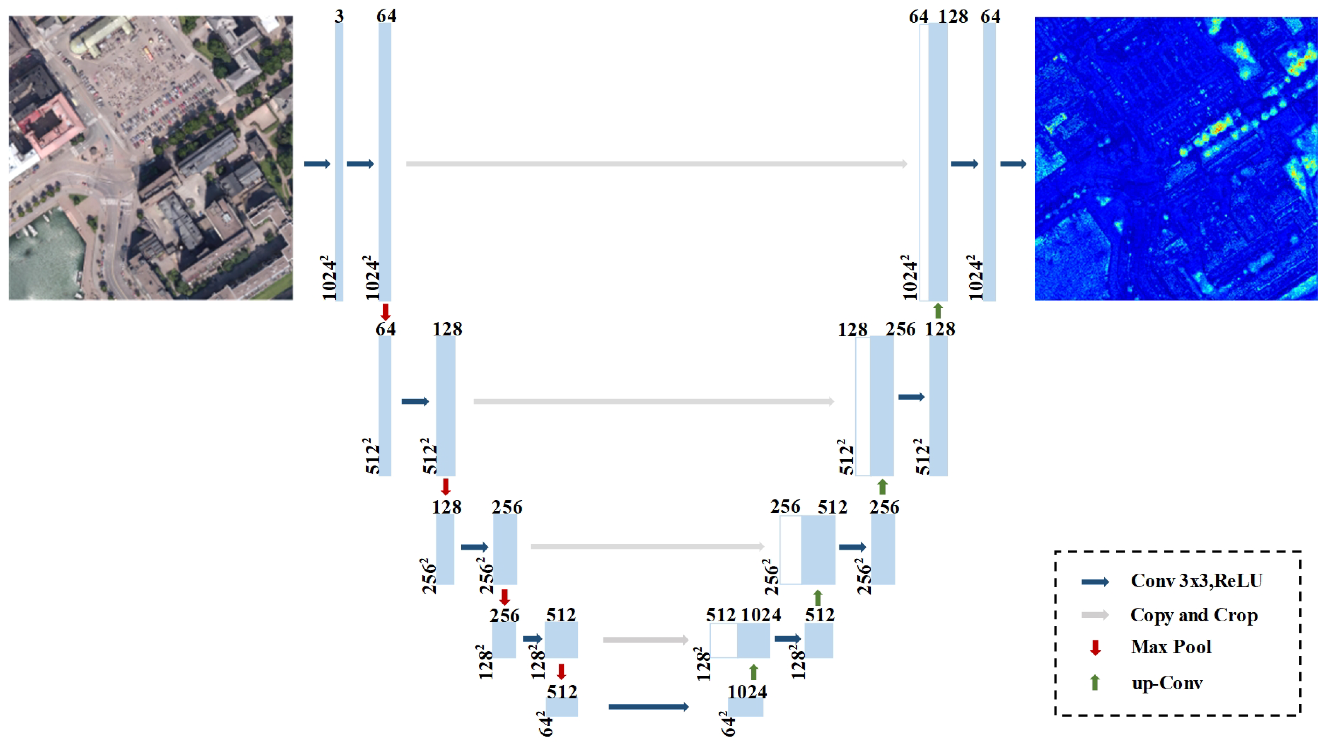
2.2. U-Net-Based 2D Texture Feature Extraction

The high-resolution texture patches of the textured urban 3D mesh contain rich semantic information. However, due to the irregular geometry of the 3D mesh, the variations in the shapes and positions of individual triangles complicate the convolutional operations applied to these texture patches. This geometric inconsistency hinders the ability of convolutional neural networks to effectively extract local features from the texture, thereby affecting the model’s performance in the task. To better exploit the texture attributes of the textured urban 3D mesh, we propose representing the texture features in a regularized form by capturing orthogonal views from a top-down perspective, as illustrated in Figure 2.

We capture high-resolution snapshots of the textured urban 3D mesh using MeshLab, with the Shading attribute set to “None” and the Color attribute set to “User-Def: White”. These snapshots provide orthogonal views of the urban scene from a top-down perspective. The orthogonal views of regions with identical urban scenes are of the same dimensions. Therefore, the input to the 2D branch consists of 1024 × 1024 three-channel images. These images are processed through a U-Net architecture to extract high-level features, with the final layer of the encoder outputting 1024 × 1024 × 64 2D high-level features. The overall framework is illustrated in Figure 3.

2.3. Multi-Scale Transformer-Based 3D Feature Extraction

To address the challenges of significant scale variation and class imbalance in textured urban 3D meshes, we propose a multi-scale feature extraction method that integrates PointNet and Transformer architectures. PointNet’s neighborhood aggregation mechanism is utilized to extract local multi-scale features, enabling the capture of fine-grained geometric details across different scales. To further enhance the representation with global contextual information, the Transformer is employed to model long-range dependencies. The input features consist of the centroid coordinates and face normal vectors of the textured urban 3D mesh. The overall architecture of this component is illustrated in the first row of Figure 1.

2.3.1. Adaptive Balanced Sampling

To ensure alignment with the input of the 2D feature extraction branch, the 3D feature extraction branch takes as input the textured urban 3D mesh patches corresponding to the overhead view. However, the number of mesh elements can vary significantly across different urban regions. Existing methods typically apply preprocessing techniques to standardize the input size when dealing with samples of varying mesh counts. Common strategies include reducing data density to maintain a consistent region size—at the cost of losing fine-grained features—or enlarging the region to preserve data density, which often leads to sparse projections in the orthographic overhead view, with some patches covering only a small portion of the image. Traditional Transformer-based models typically address variable input sizes using padding, extending data to a fixed length. However, this approach becomes computationally expensive and memory-inefficient when applied to large-scale datasets.

To address these challenges, we propose an adaptive balanced sampling strategy based on farthest point sampling, designed to uniformly sample inputs of varying sizes and ensure consistent scale changes during successive downsampling operations. This strategy enables the network to maintain uniform sampling strength, even when handling 3D meshes with significant mesh count discrepancies, thereby preventing imbalances in feature extraction due to input size variations. This approach improves the adaptability and stability of the model across different object scales.

For any given textured urban 3D mesh with a mesh count of $N_0$, we first set the mesh count after passing through the Transformer layers as $N_T$, with the number of sampling steps being k. The balanced sampling coefficient is then calculated using the following formulas:

$$\delta ={\left({\displaystyle \frac{{\mathrm{N}}_0}{N_T}}\right)}^{{\displaystyle \frac{1}{k}}}$$

(1)

The number of sampling steps k is chosen to be 3. The relationship between the number of meshes before sampling $N_i$ and the number of meshes after a single sampling step $N_{i+1}$ is given by the following formulas:

$$N_{i+1}={\displaystyle \frac{N_i}{\delta }}$$

(2)

Here, i represents the sampling step. After k sampling steps, the number of meshes decreases proportionally from the initial value $N_0$ to $N_T$, ensuring a balanced scale transformation of the textured urban 3D mesh.

The centroid coordinates $\left[X, Y, Z\right]$ and normal vector $\left[N_x, N_y, N_z\right]$ of the mesh are taken as the initial features. For the original input $M\left(N_0,6\right)$, the initial features are first encoded into a high-dimensional space through a MLP. The output dimension of the MLP is $C_0=12$. The specific formulas is as follows:

$$M_S^0=Relu\left(BN\left(MLP\left(M\right)\right)\right)$$

(3)

where $M_S^0$ represents the upsampling stage. After calculating the balanced sampling coefficient $\delta$, sampling and grouping are performed through the sampling layer and the grouping layer, respectively, as shown in Figure 4. For the sampling layer, the meshes retained after sampling, the grouping layer finds the remaining meshes in their neighborhood and groups them. The PointNet layer is then used to aggregate neighborhood features for each group, obtaining local features at different scales. After each sampling, the sample size of $M_0$ is reduced by a factor of * (denoted as the scaling factor), and the grouping and neighborhood feature aggregation process doubles the feature dimension of $M_0$, as shown in the following formulas:

$$M_S^{i+1}\left(N_{i+1}, C_{i+1}\right)=PointNet\left(Group\left(Samp\left(M_S^i\left(N_i, C_i\right)\right)\right)\right)$$

(4)

where $C_{i+1}=2·C_i$. After three iterations of sampling, grouping, and feature aggregation, the resulting $M_S^3\left(N_T, C_3\right)$ effectively represents the original input data and contains rich multi-scale features.

2.3.2. Self-Attention Global Feature Extraction

After three adaptive balanced downsampling steps, the number of meshes is reduced to our preset number $C_3$, and the feature dimension after feature aggregation is $C_3$. The aggregated features are then passed into the Transformer encoder layer, where their feature dimension is mapped to $C_T$ using learnable matrices $WQ$, $WK$, and $WV$, as follows:

$$\begin{array}{c}Q(N_T,C_T)=M_S^3(N_T,C_3)·WQ\hfill \\ K(N_T,C_T)=M_S^3(N_T,C_3)·WK\hfill \\ V(N_T,C_T)=M_S^3(N_T,C_3)·WV\hfill \end{array}$$

(5)

The self-attention matrix is obtained by multiplying the Q and K matrices as follows:

$$SA=softmax\left(Q{K}^T\right)$$

(6)

Finally, the attention matrix is multiplied by V to obtain the output of the Transformer as follows:

$$\begin{array}{c}{M}_T^i(N_T,C_T)=SA\ast \mathrm{V}\hfill \end{array}$$

(7)

It is worth noting that multi-head attention merges the final outputs along the feature dimension. We use 4 attention heads, so the output feature dimension is $CT·4$. To ensure that the output feature dimension remains within a reasonable range, we apply a fully connected layer to reduce the output feature dimension.

$$\begin{array}{c}{M}_T(N_T,C_T)=\hfill \\ \mathrm{R}\mathrm{e}lu\left(BN\left(MLP\left(ConCat(M_T^1+M_T^2+M_T^3+M_T^4)\right)\right)\right)\hfill \end{array}$$

(8)

Here, $M_T^i$ represents the output of the different attention heads, and $C_T=96$.

2.3.3. Dual Skip Connection Upsampling

Due to the significant size differences among various object categories in textured urban 3D mesh, multi-scale features play a crucial role in semantic segmentation. During the multiple downsampling stages, small-sized object features are inevitably lost. To address this issue, we employed an improved upsampling strategy that incorporates a dual skip connection module. This module uses a distance-based interpolation and hierarchical propagation strategy with dual skip connections, as shown in Figure 5.

Specifically, during the downsampling process, two mesh groups of different resolutions are obtained, denoted as $M_S^i\in {\mathbb{R}}^{N_i\times C_i}$ and $M_S^{i+1}\in {\mathbb{R}}^{N_{i+1}\times C_{i+1}}$, where $N_i>N_{i+1}$ and $C_i<C_{i+1}$. Consider an arbitrary mesh element $m_S^i$ from the group $M_S^i$. If it does not exist in $M_S^{i+1}$, an interpolation-based upsampling strategy is employed. Specifically, the three nearest neighbors of $m_S^i$ in Euclidean space within $M_S^{i+1}$—denoted as $m{1}_S^{i+1},m{2}_S^{i+1},m{3}_S^{i+1})$—are identified, and the average of their corresponding high-level features is taken as the interpolated feature for $m_S^i$, as illustrated in Figure 6. The upsampled feature set, denoted as A, maintains the enhanced point resolution while preserving the high-dimensional feature representation. This feature set is then concatenated with the original $M_S^i$ (which has the same number of elements) along the feature dimension. The fused feature representation is subsequently passed through a Multi-Layer Perceptron (MLP) to obtain the final feature embedding C, which integrates multi-scale contextual information.

$$\begin{array}{c}C=Relu\left(BN\left(MLP\left(ConCat(A, M_S^i)\right)\right)\right)\in {\mathbb{R}}^{N_i\times C_{MLP}}\hfill \end{array}$$

(9)

After obtaining the fused feature representation, the downsampled mesh group $M_S^i$, which shares the same resolution scale, is concatenated with the fused feature C to form the input for the next upsampling stage, denoted as $M_U^i$ as follows:

$$\begin{array}{c}{M}^{U_i}=ConCat(C, M_S^i)\in {\mathbb{R}}^{N_i\times C_{MLP}+C_i}\hfill \end{array}$$

(10)

This design facilitates a better balance between fine-grained local features and global contextual information, thereby enabling more effective feature propagation across different scales.

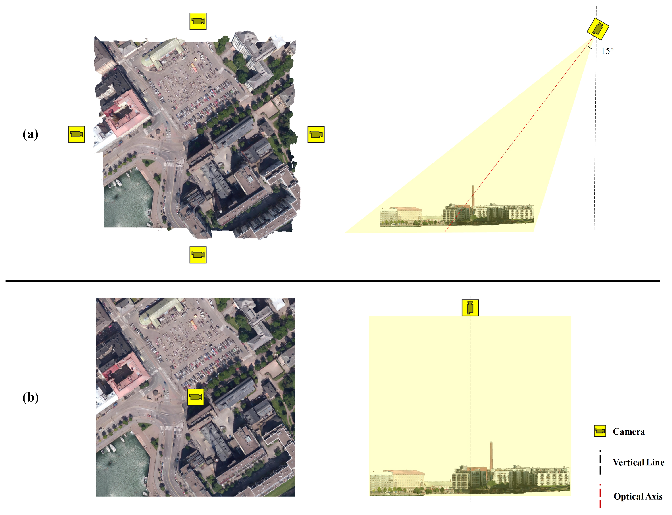
2.4. Bridge-View-Based 2D Image and 3D Mesh Alignment Algorithm

When capturing the textured 3D mesh of an urban scene, the occlusion relationship between the mesh faces for any given camera pose can be classified into full occlusion, partial occlusion, and no occlusion, as shown in Figure 7. In the SUM dataset, the 3D meshes have varied shapes, large scale differences, and are non-water-tight, making traditional methods of calculating the correspondence between 2D images and 3D meshes through camera intrinsic and extrinsic parameters both complex and computationally expensive. Determining the exact correspondence between each mesh in the textured 3D mesh and the pixels in the orthographic view is crucial for aligning 2D and 3D features. To address this, we propose a cross-modal information fusion module (Bridge of 2D–3D), designed to efficiently achieve pixel-level alignment between the 3D mesh and the 2D image, facilitating the precise alignment of cross-modal features.

Given a city scene M, which consists of n mesh faces, each mesh face is assigned a unique index number $idx$. This unique index is inherently provided by the structure of the PLY file, where each face in the mesh is stored with a sequential index. We first design a set of formulas to assign a unique RGB value to each index number, as shown in Figure 8.

We generate a unique RGB value for each face based on its index number using the following formula, where [ ] denotes the floor operation and { } denotes the modulus operation:

$$\begin{array}{c}R=[idx/{255}^2]\hfill \\ G=[\{idx/{255}^2\}/255]\hfill \\ B=\{\{idx/{255}^2\}/255\}\hfill \end{array}$$

(11)

After assigning a unique RGB value to each mesh in M, we create a Bridge M that differs from the original M solely by its RGB values. Using the same camera pose, we take snapshots of both the Bridge M and the original M in MeshLab, resulting in two images. The first image is referred to as the Bridge view, while the second image is called the Color view (as shown in Figure 9).

As illustrated in Figure 10, the proposed Bridge view serves as an intermediate bridge that enables precise pixel-level alignment between the texture image and the 3D mesh. Specifically, for any pixel $p(u_p,v_p)$ in the texture view, we locate the corresponding pixel $p_{Bridge}(u_p,v_p)$ at the same position in the Bridge view. Since both the texture view and the Bridge view share identical rendering parameters, p and $p_{Bridge}$ are guaranteed to correspond to the same mesh face—this explains the alignment process from (a) to (b). Subsequently, the RGB value $(R_p,G_p,B_p)$ of $p_{Bridge}(u_p,v_p)$ can be decoded using Formula (11) to retrieve the unique index of the associated mesh face, establishing the link between (b) and (c). Through this bridging mechanism, pixel-level correspondence between the texture image and the 3D mesh is effectively established. Moreover, this process is purely inference-based and leverages the rendering pipeline, which naturally handles occlusion relationships during the generation of the Bridge view.

Once the mesh face indices corresponding to all the pixels in the image are determined, we need to make some selections. For pixels that belong to the same mesh (i.e., those with the same RGB value in the Bridge image), we arrange them in a top-to-bottom manner and select the most representative pixel in the middle to represent the 2D feature of the mesh (as shown in Figure 11).

Through the above alignment method, we transfer the 2D features into the 3D space and merge them with the 3D features, resulting in enriched multimodal features. This fusion leads to more accurate semantic segmentation results.

3. Experiments

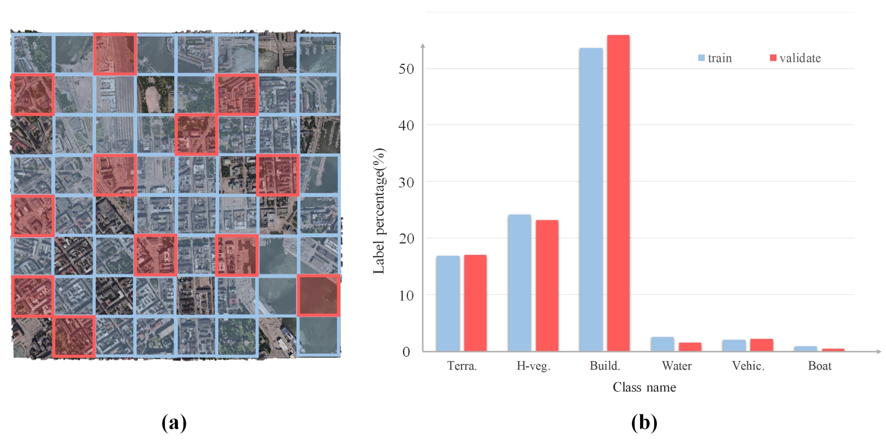
3.1. Dataset

We utilized the benchmark dataset of semantic urban meshes [42] to train and validate our proposed method. This dataset covers approximately 4 km² in Helsinki, Finland, and it includes the following six categories: ground, vegetation, buildings, water, cars, and boats. The textured mesh data were generated using Context Capture from oblique aerial images, with a ground sampling distance of 7.5 cm.

The textured mesh data is partitioned into 64 blocks, 40 of which are employed to train our network, while 12 blocks are used to validate the efficacy of the proposed method. The overall distribution of the training and testing datasets is illustrated on the left side of Figure 12. The total number of 3D mesh samples utilized in our study amounts to 14,827,376, with 11,201,466 samples designated for the training set and 3,625,910 for the testing set. We conducted a comprehensive statistical analysis of the category counts in both the training and validation datasets. The six primary label counts in the urban scene dataset are as follows: ground (1,887,520; 617,210), vegetation (2,707,067; 839,749), buildings (6,008,682; 2,027,413), water (279,316; 53,604), cars (225,962; 78,815), and boats (92,919; 9119), with data proportions depicted in the bar chart on the right side of Figure 12. The surface counts for each category are notably imbalanced, posing a significant challenge for effectively performing semantic segmentation tasks on textured meshes with such imbalanced classes. More details are shown in Figure 13.

3.2. Configurations of Multimodal Feature

We have provided detailed information on different configurations in

Table 1. Details of different configurations. cf. i: configuration i, i = 1, 2, 3, 4. *: no input; ✓: input used.

2D-Branch	3D-Branch	cf.1	cf.2	cf.3	cf.4
*	XYZ + NV	✓
RGB-tsp	XYZ + NV		✓
Per-us	XYZ + NV			✓
Ort-us	XYZ + NV				✓

. To validate the performance of the proposed method, we conducted experiments using various configurations.

In cf.1, the input data consists solely of 3D coordinates and surface normals (XYZ + Nv, 6 dimensions in total), and only the 3D feature extraction network is employed.

In cf.2, the texture information is incorporated by sampling RGB values at texture points, resulting in an input of 27 sampled RGB values concatenated with the 3D coordinates and surface normals (27 × RGB + XYZ + Nv, 81 dimensions in total), with the 3D feature extraction network solely applied.

cf.3 and cf.4 utilize both the 2D texture view (perspective and orthographic projections, respectively) and the 3D coordinates with surface normals as inputs. Feature extraction is conducted through both 2D and 3D feature extraction networks, and the resulting features are subsequently fused. The perspective view is obtained by capturing snapshots of the urban dataset using four tilted cameras positioned above the scene, resulting in perspective images representative of oblique viewing, as illustrated in Figure 14a. The orthographic view corresponds to a top-down, nadir perspective, simulating remote sensing imagery as shown in Figure 14b.

We evaluate the segmentation results using a confusion matrix. The evaluation metrics include the following: Overall Accuracy (OA), Mean Accuracy (mAcc), Mean Intersection over Union (mIoU), Recall (R), and F1 Score.

3.3. Implementation Details

Our network is implemented and fine-tuned using the deep learning framework PyTorch v2.1.0. Training and testing were conducted on a machine equipped with an NVIDIA GeForce RTX 3060 GPU. During both the training and testing phases, the learning rate was set to 0.001 and decreased by 90% every 20 epochs, with a minimum value of 0.00001. Since the model accepts a variable number of large-scale 3D meshes as input, the batch size was set to 1. Other parameters in the model, such as the number of 3D meshes fed into the Transformer layer and the number of neighbors selected for the k-NN group, were set to 4096 and 32, respectively. These values were determined through experiments considering different configurations and the processing capabilities of the hardware system. Details of the experiments and analysis for hyperparameter tuning are described in the experimental section. The initial feature encoding dimension is set to 12, and after the four stacked Transformer layers are merged and passed through the MLP, the output dimension is 96.

For data input, as shown in Figure 15, each 250 m × 250 m city scene is divided into four parts in the 2D plane. This approach helps to improve the resolution of the orthogonal view with the same size while reducing the number of 3D mesh inputs for the 3D branch, resulting in a smoother downsampling process.

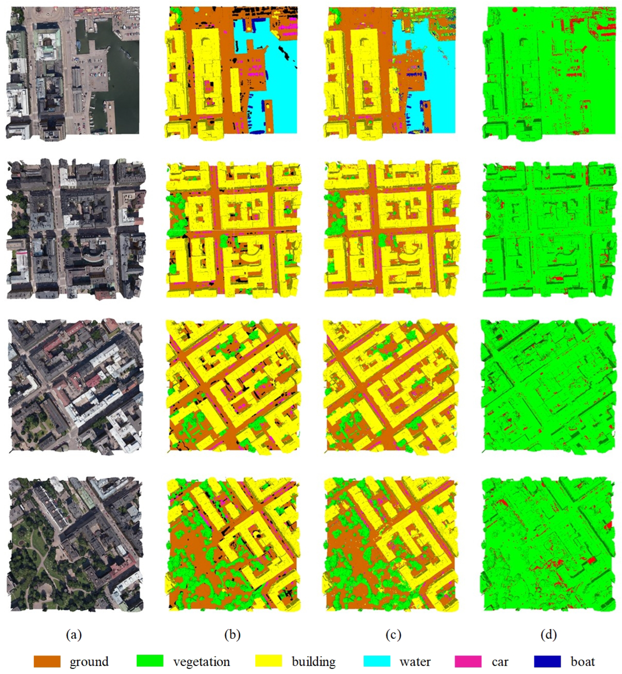
3.4. Semantic Segmentation Results of the 3D Mesh Urban Scene

Figure 16 illustrates some semantic mesh segmentation results obtained using the proposed method under configuration cf.4 As shown in Figure 16d, due to the class imbalance in the training and validation datasets, prediction errors primarily occur in the water, car, and boat classes.

According to our experimental results, the building class consistently performs the best, while the boat class shows the worst performance, with significant variability in its metrics. This is due to the large-scale disparity in the boat class. The large-scale boat objects have similar appearances in the orthogonal view under the bird’s eye perspective as the small-scale building class, while the small-scale boats share similarities in both the orthogonal view and spatial geometry with the car class.

3.5. Evaluation of Competition Methods

To evaluate the performance of the proposed method, Rongting Zhang et al. introduced state-of-the-art methods, which also used the SUM dataset utilized in this paper. Additionally, Rongting Zhang et al. compared their approach with several point-based deep learning methods, including PointNet [43], ++ [44], SPG [45], RandLA-Net [46], KPConv [26], and DGCNN [47]. Transformer-based point cloud segmentation methods [48] were also compared with our approach.

As shown in the comparison results in

Table 2. Accuracy comparisons among different methods. The results reported in this table are the IOU (%) per class, OA (%), mAcc (%), mIoU (%), and mF1 (%).

Method	Terra.	H-veg.	Build.	Water	Vehic.	Boat	OA	mAcc	mIoU	mF1
Ours	79.6	89.0	94.1	83.3	51.3	30.1	94.0	81.5	71.4	79.7
PT	78.4	58.0	80.1	95.6	1.7	28.5	85.2	66.5	57.1	66.0
PointNet	56.3	14.9	66.7	83.8	0.0	0.0	71.4	46.1	36.9	44.6
PointNet++	68.0	73.1	84.2	69.9	0.5	1.6	85.5	57.8	49.5	57.1
SPG	56.4	61.8	87.4	36.5	34.4	6.2	79.0	64.8	47.1	59.6
RandLA-Net	38.9	59.6	81.5	27.7	22.0	2.1	74.9	53.3	38.6	49.9
KPConv	86.5	88.5	92.7	77.7	54.3	13.3	93.3	73.3	68.8	76.7

, the method proposed in this paper outperforms all other methods. Compared to others, our method achieves an improvement of 13.2% in average accuracy (mAcc), 2.6% in mean intersection over union (mIoU), and 13.7% in F1 Score.

In Table 2, KPConv emerges as one of the most competitive baseline methods due to its strong geometric modeling capability. It achieves high performance across multiple classes and records an overall accuracy (OA) of 93.3%. Our method further improves this result, reaching an OA of 94.0%. Although the numerical difference in OA is relatively small, it is important to note that OA may not fully reflect performance differences on imbalanced datasets, as it is heavily influenced by dominant classes such as Buildings and Vegetation.To provide a more comprehensive evaluation, we report additional metrics, including the mean Intersection-over-Union (mIoU), mean Accuracy (mAcc), and mean F1 Score (mF1). Our model significantly outperforms KPConv by +2.6% in mIoU, +8.2% in mAcc, and +3.0% in mF1, indicating a more balanced and robust segmentation performance across all categories. Specifically, our approach shows superior results in texture-dependent and underrepresented classes such as Boat, Water, and Vehicle, which remain challenging for geometry-only methods like KPConv. These improvements demonstrate the effectiveness of our multimodal fusion framework in integrating high-resolution texture features with 3D geometry, leading to enhanced semantic understanding in complex urban environments.

3.6. Evaluation of Ablation Study

To investigate the impact of multimodal features compared to single-modal features on segmentation performance, we designed four experimental configurations for texture information input.

Table 3. Accuracy comparisons among different inputs. The results reported in this table are the IOU (%) per class, OA (%), mAcc (%), mIoU (%), and mF1 (%).

Texture Input Format	Terra.	H-veg.	Build.	Water	Vehic.	Boat	OA	mAcc	mIoU	mF1
cf.1	70.2	75.3	79.8	50.1	30.4	10.2	85.5	45.2	60.1	50.3
cf.2	77.9	78.4	88.1	56.0	40.3	15.6	92.2	73.4	59.4	65.6
cf.3	74.5	81.1	88.4	47.5	42.1	40.1	91.3	72.5	62.4	70.3
cf.4	79.6	89.0	94.1	83.3	51.3	30.1	94.0	81.5	71.4	79.7

shows that the single-modal data, based solely on geometric features, achieved an overall accuracy (OA) of 85.5%. Nevertheless, the mIoU and mAcc were relatively low, at 45.2% and 60.1%, respectively, primarily due to label imbalance.

After introducing multimodal data, the overall accuracy (OA) significantly improved from 85.5% to 94.0%. The mean Intersection over Union (mIoU) increased from 45.2% to 71.4%, and the mean Accuracy (mAcc) rose from 60.1% to 81.5%. More specifically, there was a notable improvement in low-sample categories, such as the mIoU of the boat category increasing from 10.2% to 30.1%. These results demonstrate the critical role of multimodal features in segmentation tasks. Specifically, for distinguishing categories with similar geometric information, such as vehicles and boats (mIoU improved from 30.4% to 51.3%) or ground and water surfaces (mIoU improved from 50.1% to 83.3%), the introduction of multimodal features provided effective support, significantly enhancing segmentation performance.

3.6.1. Impact of Using Orthogonal Views to Replace the RGB Values of Texture Sampling Points

Texture sampling points are extracted from the corresponding texture image of the textured 3D mesh using a specific algorithm, maximizing the coverage of triangles to obtain RGB values that best represent their texture features. However, the effectiveness of texture sampling points is subject to the following limitations:

(1)

Feature dimensionality and sampling points. The feature dimensionality of texture sampling points is proportional to the number of selected points. More sampling points increase the texture representativeness by covering the entire mesh more completely. For a mesh with n sampling points, the texture feature dimension is $3n$. Since urban scenes typically involve large-scale textured 3D meshes with numerous mesh faces, using a large number of sampling points to cover the entire mesh leads to an explosion in feature dimensions.

(2)

Variation in mesh sizes. Different objects in urban scene textured 3D meshes have varying levels of detail and size, which results in texture images with significantly different pixel counts. For a fixed number of texture sampling points, the coverage and texture representativeness differ greatly across meshes of different sizes.

(3)

Noise in texture images. Texture images often contain noise, which complicates the process. When sampling points are located in noisy regions, the extracted RGB values may differ substantially from the mesh’s average RGB values, leading to inaccurate results. Even if the sampling points fall on noise-free regions, the relative position relationships between the sampling points are still disrupted. Since different combinations of RGB values in different positions can represent different features, discrete texture sampling points may fail to properly represent the texture features of urban scenes.

Based on the above issues, as shown in Table 3, when texture sampling point RGB values were used as 2D features for the textured 3D mesh, the overall accuracy reached 92.2%, which is a good result. However, the mean intersection over union (mIoU) was only 59.4%, indicating that texture sampling points do not effectively replace the 2D texture features of the mesh. When orthogonal views from a top-down perspective were used as 2D features, the overall accuracy increased to 94.0%, and the mIoU reached 71.4%, a 10% improvement. The positive effect of using orthogonal views instead of texture sampling points is evident.

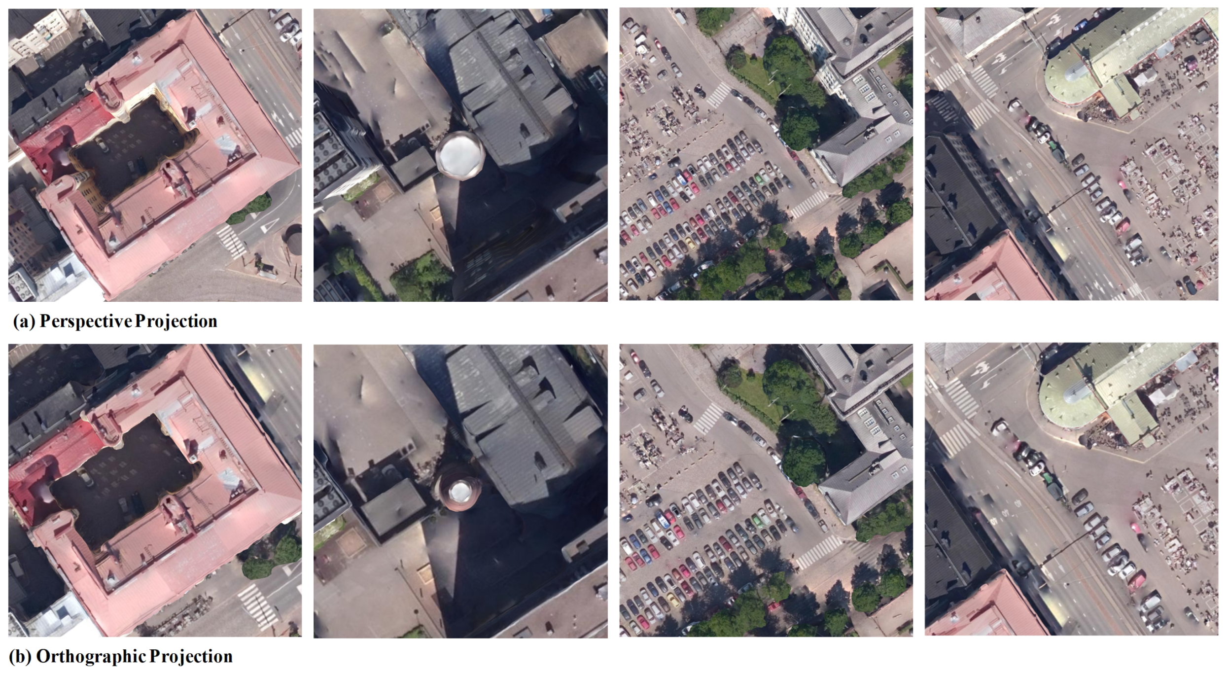
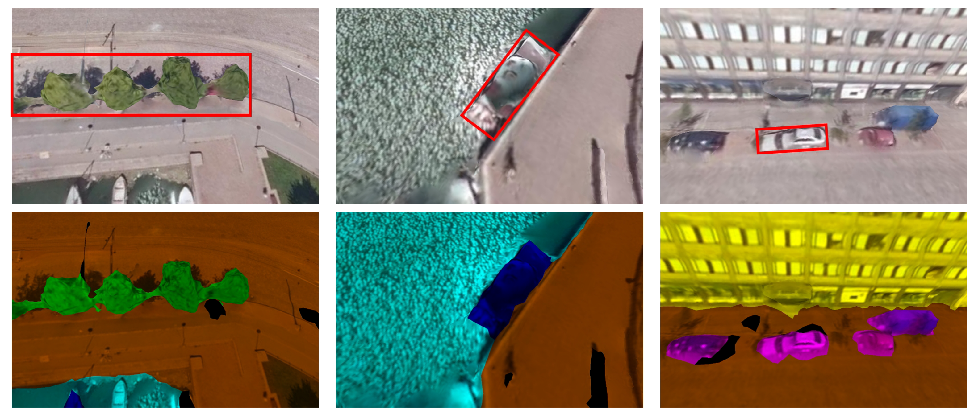
3.6.2. Impact of Orthogonal Views Compared to Perspective Views

To further explore the effect of different perspectives on the segmentation results, we introduced perspective views from multiple angles. To capture as many meshes in the urban scene as possible and ensure that at least one pixel corresponds to each mesh, we captured the perspective views of the urban scene from four edge-centers, at a 15° tilt angle from a top-down position. Each scene corresponds to four perspective views.

Since the appearance of perspective views depends on the camera angle, different shooting angles can cause changes in the projection shape, size, and relative position of objects. Additionally, objects far from the viewpoint may undergo distortions (e.g., rectangles turning into trapezoids), as perspective projections distort 3D objects when mapped onto a 2D plane. When capturing urban scenes from the SUM dataset using MeshLab, perspective views distort planes parallel to the viewpoint direction, leading to severe distortions in building walls and unclear boundaries between buildings and the ground. The overall accuracy for the perspective view was 91.3%, with an mIoU of 62.4%. Compared to the orthogonal view from a top-down perspective, this result was less accurate.

4. Discussion

4.1. Impact of the Mesh Coverage Rate in Texture Views on Segmentation Performance

We define the mesh coverage rate in the texture view as the proportion of mesh faces in a given textured urban 3D mesh that are captured by at least one pixel in the rendered texture image (i.e., each pixel is associated with a uniquely indexed mesh face). In the 2D feature extraction branch, neither perspective nor orthographic projection can guarantee that every mesh face is covered by at least one corresponding pixel (i.e., achieving 100% coverage), which is critical for further improving semantic segmentation accuracy.

As shown in Figure 17a, perspective projection mimics human visual perception by simulating a “near-large, far-small” effect, thereby enhancing spatial depth perception. However, it does not preserve geometric proportions and may introduce significant distortion, particularly when the viewing angle deviates or when objects are far from the camera.

As shown in Figure 17b, orthographic projection preserves the geometric shape and proportions of objects, as all projection rays are parallel and perpendicular to the projection plane. This projection ensures good geometric consistency. However, due to the absence of perspective scaling, it tends to cause overlapping objects along the projection direction in large-scale urban scenes, leading to local occlusion and information loss. As a result, the mesh coverage rate in orthographic texture views is generally lower than that of perspective views.

During the multimodal feature fusion stage, mesh faces that are not captured in the texture view cannot obtain the corresponding high-resolution 2D texture features and must rely solely on their 3D geometric features for semantic prediction. This results in incomplete feature fusion and may limit segmentation performance. Therefore, generating texture views with higher mesh coverage rates is an important direction for future research.

4.2. Discussion of the Impact of Virtual vs. Real Urban Scenes on Segmentation Performance

In this study, the texture views are generated from virtual urban scenes based on the SUM dataset using rendering tools such as MeshLab. However, during the production of the SUM dataset, we observed that certain objects with complex geometric structures—such as tall vegetation, vehicles, and ships—exhibited noticeable structural deformations or distortions during the 3D modeling process, as shown in Figure 18. These artifacts may affect the visual realism and semantic consistency of the texture images, thereby influencing the accuracy and generalizability of the segmentation results.

Future research can further improve the practicality and accuracy of the proposed method from two perspectives. On the one hand, high-precision 3D reconstruction techniques can be introduced to enhance the geometric fidelity of the 3D models, thereby reducing structural distortions commonly observed in complex objects during the modeling process. On the other hand, real remote sensing images can be employed to replace the virtual texture views, enabling the generation of more realistic and discriminative 2D texture information. This would enhance the expressiveness of multimodal feature fusion and improve the accuracy of semantic segmentation.

5. Conclusions

Although textured urban 3D meshes offer a more detailed and structured representation compared to traditional 3D formats such as point clouds, research on semantic segmentation of textured meshes in complex urban scenes remains in its early stages. In this paper, we propose a multimodal feature fusion network that integrates 3D geometric structures with high-resolution 2D texture imagery for the semantic segmentation of textured urban 3D meshes. To effectively leverage the rich texture information inherent in textured meshes, we generate orthographic texture views from a top-down perspective. High-level features are then independently extracted from both 2D and 3D modalities.

To enable precise and efficient multimodal correspondence, we introduce a cross-modal information fusion module, termed the Bridge of 2D–3D, which aligns the high-level 2D features with the 3D mesh structure. This alignment results in a comprehensive and semantically enriched feature representation. Compared with state-of-the-art point cloud-based deep learning methods and other advanced approaches, our method achieves superior performance, with an overall accuracy (OA) of 94.0% and a mean Intersection over Union (mIoU) of 71.4%. These results demonstrate the effectiveness of the proposed framework in improving the accuracy of semantic mesh segmentation.

Future research will be directed toward the following three aspects.

(1)

Enhanced view coverage: We will explore the use of texture images generated from additional virtual viewpoints to improve mesh coverage in texture space, thereby enhancing the model’s perception of occluded and structurally complex regions.

(2)

We plan to investigate more expressive multimodal fusion strategies by jointly embedding high-level 2D texture features and 3D geometric features (e.g., coordinates and normal vectors) into a unified network to better capture multi-scale and global contextual information.

(3)

With the ongoing advances in 3D reconstruction techniques and remote sensing imagery, we aim to replace synthetic texture views with real-world remote sensing images. This transition is expected to significantly improve the realism and semantic expressiveness of the texture views, thereby enhancing the generalization capability and practical value of the proposed method in real-world urban scenarios.

References

- Chen, Z.; Deng, L.; Luo, Y.; Li, D.; Junior, J.M.; Gonçalves, W.N.; Nurunnabi, A.A.M.; Li, J.; Wang, C.; Li, D. Road Extraction in Remote Sensing Data: A Survey. Int. J. Appl. Earth Obs. Geoinf. 2022, 112, 102833. [Google Scholar] [CrossRef]
- Chen, Y.; Feng, M. Urban form simulation in 3D based on cellular automata and building objects generation. Build. Environ. 2022, 226, 109727. [Google Scholar] [CrossRef]
- Yang, X. Urban Remote Sensing: Monitoring, Synthesis and Modeling in the Urban Environment, 2nd ed.; Wiley-Blackwell: Hoboken, NJ, USA, 2021. [Google Scholar] [CrossRef]
- Hong, Z.; Yang, Y.; Liu, J.; Jiang, S.; Pan, H.; Zhou, R.; Zhang, Y.; Han, Y.; Wang, J.; Yang, S.; et al. Enhancing 3D Reconstruction Model by Deep Learning and Its Application in Building Damage Assessment after Earthquake. Appl. Sci. 2022, 12, 9790. [Google Scholar] [CrossRef]
- Zhang, J.; Zhao, X.; Chen, Z.; Lu, Z. A review of deep learning-based semantic segmentation for point cloud. IEEE Access 2019, 7, 179118–179133. [Google Scholar] [CrossRef]
- Liu, W.; Sun, J.; Li, W.; Hu, T.; Wang, P. Deep Learning on Point Clouds and Its Application: A Survey. Sensors 2019, 19, 4188. [Google Scholar] [CrossRef] [PubMed]
- Gupta, A.; Byrne, J.; Moloney, D.; Watson, S.; Yin, H. Tree Annotations in LiDAR Data Using Point Densities and Convolutional Neural Networks. IEEE Trans. Geosci. Remote Sens. 2020, 58, 971–981. [Google Scholar] [CrossRef]
- Hu, X.; Yuan, Y. Deep-learning-based classification for DTM extraction from ALS point cloud. Remote Sens. 2016, 8, 730. [Google Scholar] [CrossRef]
- Rizaldy, A.; Persello, C.; Gevaert, C.; Oude Elberink, S.; Vosselman, G. Ground and multi-class classification of airborne laser scanner point clouds using fully convolutional networks. Remote Sens. 2018, 10, 1723. [Google Scholar] [CrossRef]
- Ma, L.; Li, Y.; Li, J.; Tan, W.; Yu, Y.; Chapman, M.A. Multi-scale point-wise convolutional neural networks for 3D object segmentation from LiDAR point clouds in large-scale environments. IEEE Trans. Intell. Transp. Syst. 2019, 22, 821–836. [Google Scholar] [CrossRef]
- Wu, W.; Qi, Z.; Fuxin, L. Pointconv: Deep convolutional networks on 3d point clouds. In Proceedings of the IEEE/CVF Conference on Computer Vision and Pattern Recognition, Long Beach, CA, USA, 15–20 June 2019; pp. 9621–9630. [Google Scholar]
- Rouhani, M.; Lafarge, F.; Alliez, P. Semantic segmentation of 3D textured meshes for urban scene analysis. ISPRS J. Photogramm. Remote Sens. 2017, 123, 124–139. [Google Scholar] [CrossRef]
- Tutzauer, P.; Laupheimer, D.; Haala, N. Semantic Urban Mesh Enhancement Utilizing a Hybrid Model. ISPRS Ann. Photogramm. Remote Sens. Spat. Inf. Sci. 2019, 4, 175–182. [Google Scholar] [CrossRef]
- Cun, Y.L.; Boser, B.; Denker, J.S.; Howard, R.E.; Habbard, W.; Jackel, L.D.; Henderson, D. Handwritten digit recognition with a back-propagation network. In Advances in Neural Information Processing Systems 2; David, S.T., Ed.; Morgan Kaufmann Publishers Inc.: San Francisco, CA, USA, 1990; pp. 396–404. [Google Scholar]
- Krizhevsky, A.; Sutskever, I.; Hinton, G.E. ImageNet classification with deep convolutional neural networks. Commun. ACM 2012, 60, 84–90. [Google Scholar] [CrossRef]
- Simonyan, K.; Zisserman, A. Very deep convolutional networks for large-scale image recognition. In Proceedings of the 3rd International Conference on Learning Representations, San Diego, CA, USA, 7–9 May 2015. [Google Scholar]
- Szegedy, C.; Liu, W.; Jia, Y.; Sermanet, P.; Reed, S.; Anguelov, D.; Erhan, D.; Vanhoucke, V.; Rabinovich, A. Going deeper with convolutions. In Proceedings of the IEEE Conference on Computer Vision and Pattern Recognition, Boston, MA, USA, 7–12 June 2015; pp. 1–9. [Google Scholar]
- Lee, J.-S.; Park, T.-H. Fast road detection by cnn-based camera–lidar fusion and spherical coordinate transformation. IEEE Trans. Intell. Transp. Syst. 2021, 22, 5802–5810. [Google Scholar] [CrossRef]
- Gu, S.; Lu, T.; Zhang, Y.; Alvarez, J.M.; Yang, J.; Kong, H. 3-D LiDAR + monocular camera: An inverse-depth-induced fusion framework for urban road detection. IEEE Trans. Intell. Veh. 2018, 3, 351–360. [Google Scholar] [CrossRef]
- Qi, X.; Liao, R.; Jia, J.; Fidler, S.; Urtasun, R. 3d graph neural networks for rgbd semantic segmentation. In Proceedings of the IEEE International Conference on Computer Vision, Honolulu, HI, USA, 21–26 July 2017; pp. 5199–5208. [Google Scholar]
- Dai, A.; Nießner, M. 3dmv: Joint 3d-multi-view prediction for 3d semantic scene segmentation. In Proceedings of the European Conference on Computer Vision (ECCV), Munich, Germany, 8–14 September 2018; pp. 452–468. [Google Scholar]
- Yang, F.; Wang, H.; Jin, Z. A fusion network for road detection via spatial propagation and spatial transformation. Pattern Recognit. 2020, 100, 107141. [Google Scholar] [CrossRef]
- Su, H.; Jampani, V.; Sun, D.; Maji, S.; Kalogerakis, V.; Yang, M.-H.; Kautz, J. SPLATNet: Sparse lattice networks for point cloud processing. In Proceedings of the IEEE Conference on Computer Vision and Pattern Recognition, Salt Lake City, UT, USA, 19–21 June 2018. [Google Scholar]
- Masci, J.; Boscaini, D.; Bronstein, M.; Vandergheynst, P. Geodesic convolutional neural networks on riemannian manifolds. In Proceedings of the IEEE International Conference on Computer Vision Workshops, Washington, DC, USA, 7–13 December 2015; pp. 37–45. [Google Scholar]
- Hanocka, R.; Hertz, A.; Fish, N.; Giryes, R.; Fleishman, S.; Cohen-Or, D. Meshcnn: A network with an edge. ACM Trans. Graph. 2019, 38, 1–12. [Google Scholar] [CrossRef]
- Thomas, H.; Qi, C.R.; Deschaud, J.E.; Marcotegui, B.; Goulette, F.; Guibas, L.J. Kpconv: Flexible and deformable convolution for point clouds. In Proceedings of the IEEE/CVF International Conference on Computer Vision, Seoul, Republic of Korea, 27 October–2 November 2019; pp. 6411–6420. [Google Scholar]
- Vaswani, A.; Shazeer, N.; Parmar, N.; Uszkoreit, J.; Jones, L.; Gomez, A.N.; Kaiser, Ł.; Polosukhin, I. Attention is all you need. Adv. Neural Inf. Process. Syst. 2017, 30. [Google Scholar] [CrossRef]
- Dosovitskiy, A.; Springenberg, J.T.; Riedmiller, M.; Brox, T. Discriminative unsupervised feature learning with convolutional neural networks. Adv. Neural Inf. Process. Syst. 2014, 27, 766–774. [Google Scholar] [CrossRef] [PubMed]
- Radford, A.; Kim, J.W.; Hallacy, C.; Ramesh, A.; Goh, G.; Agarwal, S.; Sastry, G.; Askell, A.; Mishkin, P.; Clark, J.; et al. Learning Transferable Visual Models From Natural Language Supervision. In Proceedings of the 38th International Conference on Machine Learning, PMLR, Virtual, 18–24 July 2021; pp. 8748–8763. [Google Scholar]
- Zhou, Y.; Tuzel, O. VoxelNet: End-to-End Learning for Point Cloud Based 3D Object Detection. In Proceedings of the 2018 IEEE/CVF Conference on Computer Vision and Pattern Recognition, Salt Lake City, UT, USA, 18–22 June 2018; pp. 4490–4499. [Google Scholar]
- Lai, X.; Liu, J.; Jiang, L.; Wang, L.; Zhao, H.; Liu, S.; Qi, X.; Jia, J. Stratified transformer for 3d point cloud segmentation. In Proceedings of the IEEE/CVF Conference on Computer Vision and Pattern Recognition, New Orleans, LA, USA, 19–20 June 2022; pp. 8500–8509. [Google Scholar]
- Dai, Z.; Yang, Z.; Yang, Y.; Carbonell, J.; Le, Q.V.; Salakhutdinov, R. Transformer-XL: Attentive language models beyond a fixed-length context. arXiv 2019, arXiv:1901.02860. [Google Scholar]
- Yang, Z.; Dai, Z.; Yang, Y.; Carbonell, J.; Salakhutdinov, R.R.; Le, Q.V. Xlnet: Generalized autoregressive pretraining for language understanding. Adv. Neural Inf. Process. Syst. 2019, 32. [Google Scholar] [CrossRef]
- Parmar, N.; Vaswani, A.; Uszkoreit, J.; Kaiser, L.; Shazeer, N.; Ku, A.; Tran, D. Image transformer. In Proceedings of the International Conference on Machine Learning, Stockholm, Sweden, 10–15 July 2018; pp. 4055–4064. [Google Scholar]
- Carion, N.; Massa, F.; Synnaeve, G.; Usunier, N.; Kirillov, A.; Zagoruyko, S. End-to-end object detection with transformers. In Proceedings of the European Conference on Computer Vision, Glasgow, UK, 23–28 August 2020; pp. 213–229. [Google Scholar]
- Dosovitskiy, A.; Beyer, L.; Kolesnikov, A.; Weissenborn, D.; Zhai, X.; Unterthiner, T.; Dehghani, M.; Minderer, M.; Heigold, G.; Gelly, S.; et al. An image is worth 16x16 words: Transformers for image recognition at scale. arXiv 2020, arXiv:2010.11929. [Google Scholar]
- Hu, H.; Zhang, Z.; Xie, Z.; Lin, S. Local relation networks for image recognition. In Proceedings of the IEEE/CVF International Conference on Computer Vision, Seoul, Republic of Korea, 27 October–2 November 2019; pp. 3464–3473. [Google Scholar]
- Ramachandran, P.; Parmar, N.; Vaswani, A.; Bello, I.; Levskaya, A.; Shlens, J. Stand-alone self-attention in vision models. Adv. Neural Inf. Process. Syst. 2019, 32, 3–5. [Google Scholar]
- Zhao, H.; Jia, J.; Koltun, V. Exploring self-attention for image recognition. In Proceedings of the IEEE/CVF Conference on Computer Vision and Pattern Recognition, Seattle, WA, USA, 13–19 June 2020; pp. 10076–10085. [Google Scholar]
- Xie, S.; Liu, S.; Chen, Z.; Tu, Z. Attentional shapecontextnet for point cloud recognition. In Proceedings of the IEEE Conference on Computer Vision and Pattern Recognition, Salt Lake City, UT, USA, 18–23 June 2018; pp. 4606–4615. [Google Scholar]
- Zhang, C.; Wan, H.; Liu, S.; Shen, X.; Wu, Z. Pvt: Point-voxel transformer for 3d deep learning. arXiv 2021, arXiv:2108.06076. [Google Scholar]
- Gao, W.; Nan, L.; Boom, B.; Ledoux, H. SUM: A benchmark dataset of semantic urban meshes. ISPRS J. Photogramm. Remote Sens. 2021, 179, 108–120. [Google Scholar] [CrossRef]
- Qi, C.R.; Su, H.; Mo, K.; Guibas, L.J. Pointnet: Deep learning on point sets for 3d classification and segmentation. In Proceedings of the IEEE Conference on Computer Vision and Pattern Recognition, Honolulu, HI, USA, 21–26 July 2017; pp. 652–660. [Google Scholar]
- Qi, C.R.; Yi, L.; Su, H.; Guibas, L.J. Pointnet++: Deep hierarchical feature learning on point sets in a metric space. In Proceedings of the Advances in Neural Information Processing Systems, Long Beach, CA, USA, 4–9 December 2017; Volume 30. [Google Scholar]
- Landrieu, L.; Simonovsky, M. Large-scale point cloud semantic segmentation with superpoint graphs. In Proceedings of the IEEE Conference on Computer Vision and Pattern Recognition, Salt Lake City, UT, USA, 18–23 June 2018; pp. 4558–4567. [Google Scholar]
- Hu, Q.; Yang, B.; Xie, L.; Rosa, S.; Guo, Y.; Wang, Z.; Trigoni, N.; Markham, A. Randla-net: Efficient semantic segmentation of large-scale point clouds. In Proceedings of the IEEE/CVF Conference on Computer Vision and Pattern Recognition, Seattle, WA, USA, 13–19 June 2020; pp. 11108–11117. [Google Scholar]
- Wang, Y.; Sun, Y.; Liu, Z.; Sarma, S.E.; Bronstein, M.M.; Solomon, J.M. Dynamic graph cnn for learning on point clouds. ACM Trans. Graph. 2019, 38, 1–12. [Google Scholar] [CrossRef]
- Zhao, H.; Jiang, L.; Jia, J.; Torr, P.H.; Koltun, V. Point Transformer. In Proceedings of the IEEE/CVF International Conference on Computer Vision (ICCV), Montreal, QC, Canada, 10–17 October 2021; pp. 16259–16268. [Google Scholar]