Parametric Representation of Tropical Cyclone Outer Radical Wind Profile Using Microwave Radiometer Data

Abstract

The Soil Moisture Active Passive (SMAP) satellite can measure sea surface winds under tropical cyclone (TC) conditions with its L-band microwave radiometer, without being affected by rainfall or signal saturation. Through the statistical analysis of SMAP data, this study aims to develop radial wind profile models for the TC outer area whose distance from TC center is larger than the radius of maximum wind ($R_{\mathrm{m}}$). A total of 196 TC cases observed by SMAP were collected between 2015 and 2020, and their intensities range from tropical storm to category 5. Based on the wind and radius data, the key model parameters $\alpha$ and $\beta$ were fitted through the Rankine vortex model and the tangential wind profile (TWP) Gaussian model, respectively. $\alpha$ and $\beta$ control the rate of change of the tangential wind speed with radius. Subsequently, for the parametric representation of $\alpha$ and $\beta$, we extracted some TC wind filed parameters, such as maximum wind speed ($U_{\mathrm{m}}$), $R_{\mathrm{m}}$, the average wind speed at $R_{\mathrm{m}}$ ($U_{\mathrm{ma}}$), and the average radius of 17 m/s ($R_{17}$) and examined the relationship between $U_{\mathrm{ma}}$ and $U_{\mathrm{m}}$, the relationship between $R_{\mathrm{m}}$ and $R_{17}$, the relationship between $\alpha$, $U_{\mathrm{m}}$ and $R_{\mathrm{m}}$, and the relationship between $\beta$, $U_{\mathrm{m}}$ and $R_{\mathrm{m}}$. According to the results, the new radial wind profile models were proposed, i.e., SMAP Rankine Model-4 (SRM-4), SMAP Rankine Model-5 (SRM-5), and SMAP Gaussian Model-1 (SGM-1). A significant advantage of these models is that they can simulate average wind distribution through the conversion from $U_{\mathrm{m}}$ to $U_{\mathrm{ma}}$. Finally, comparisons were made between the new models and existing SRM-1, SRM-2, and SRM-3, according to the Advanced Microwave Scanning Radiometer 2 (AMSR-2) measurements of 126 TC cases. The results demonstrate that the SRM-4 simulated the radial wind profile best overall, with the lowest root mean-square error (RMSE) of 5.57 m/s, due to replacing the parameter $U_{\mathrm{m}}$ with $U_{\mathrm{ma}}$, using Rankine vortex for α parameterization and modeling with adequate data. Moreover, the models outperform in the Atlantic Ocean, with a RMSE of 5.37 m/s. The new models have the potential to make a contribution to the study of ocean surface dynamics and be used for forcing numerical models under TC conditions.

1. Introduction

Tropical cyclones (TC) are a destructive weather system, causing strong wind, huge waves, intense rainfall, and storm surges [1,2,3]. TC ocean surface wind fields are relevant to several oceanic and atmospheric variables, such as heat, moisture, and momentum fluxes, which are important driving factors for atmospheric numerical models to guide TC evolution forecasting and risk assessment [4,5,6]. Thus, it is a key research area to investigate the characteristics of TC wind field and the methodology to estimate them in the aspects of intensity, size, structure, and distribution [7,8,9,10,11].

In the TC system, along the radial direction, the ocean surface wind speeds increase from central minimum to eyewall maximum and then decay with an increasing radius (R). The radial wind profile is a useful tool to describe this variation [12,13]. The parametric representation of wind profiles is an active area of research [14]. With the improvement in numerical simulation and the accumulation of observations, more and more parametric models have been established to compute wind profiles, such as the Holland hurricane model, the tangential wind profile (TWP) Gaussian model, the Gauss vortex model, the Rankine vortex model, and their modified versions [12,15,16,17,18]. Their advantage is that one can construct the entire wind field simply with limited observations, such as maximum wind speed ($U_{\mathrm{m}}$) and its radius ($R_{\mathrm{m}}$). Moreover, by adjusting the decay exponent (α), the modified Rankine vortex model has better performance than the pure Rankine vortex model, because different TC intensities correspond to different decay exponents.

With the development of remote sensing techniques, spaceborne active and passive microwave radars have been employed day and night to monitor TC systems with a large swath. For example, synthetic aperture radar (SAR) with a cross-polarization mode can retrieve wind speeds up to about 70 m/s at a high spatial resolution [19,20]. The L-band radiometers, such as the Soil Moisture Active Passive (SMAP) and the Soil Moisture and Ocean Salinity (SMOS), can also measure wind speeds in intense tropical and extratropical storms [21,22,23,24]. Its spatial resolution is not as high as SAR; however, the signal is not affected by rainfall and thermal noise [25,26,27,28].

Up to now, abundant satellite observations have become new data sources for modifying TC parametric wind filed models [29,30]. For example, based on 16 RADARSAT-2 Scan-SAR images, the Symmetric Hurricane Estimates for Wind (SHEW) model was developed by combining the Rankine vortex model and the reference ellipse [31]. The radial distributions were within 150 km from the hurricane centers. By fitting this model to the SAR retrieved wind field, one can derive five TC morphology parameters: ellipse major axis, ellipse minor axis, $U_{\mathrm{m}}$, $R_{\mathrm{m}}$ and α of the Rankine vortex, and then use them to estimate hurricane wind directions with the inflow angle model. Based on 11 Sentinel-1 images, Wang et al. proposed the TWP model, as a piecewise Gaussian-like function [17]. The model parameters a and b (we named it $\beta$ in our new model), corresponding to R ≤ $R_{\mathrm{m}}$ and $R_{\mathrm{m}}$ < R < 150 km, were fitted with the azimuth-averaged wind speeds. In their work, a and b were related to three TC intensity categories: the Small ($U_{\mathrm{m}}$ < 33.1 m/s), the Moderate (33.1 m/s ≤ $U_{\mathrm{m}}$ < 49.2 m/s), and the Major ($U_{\mathrm{m}}$ ≥ 49.2 m/s). However, for these categories, the corresponding mean b values were 0.99, 1.01, and 0.93, respectively, which were not dependent on intensity categories. In addition, the relationship between b and $U_{\mathrm{m}}$ was ambiguous for the collected profiles in the Small and Moderate categories. This implies that the TWP model may have large errors when estimating TC outer (R $\ge$ $R_{\mathrm{m}}$) wind field just with $U_{\mathrm{m}}$ and $R_{\mathrm{m}}$. In summary, when using the SHEW model and the TWP model to estimate TC wind fields, both need initial entire observed wind fields to fit α, a, and b. This raises the question: since wind fields have been observed, why does one estimate them again?

To solve this problem above, we had proposed SAR-data-based and SMAP-data-based Rankine vortex models by establishing empirical functions between α, $U_{\mathrm{m}}$, and $R_{\mathrm{m}}$ [32,33,34]. The Rankine model for outer wind field is $U=U_{\mathrm{m}}{(R_{\mathrm{m}}/R)}^{\alpha }$. The models can estimate TC outer wind profile, if $U_{\mathrm{m}}$ and $R_{\mathrm{m}}$ are known. However, the modeling process still has two problems. Firstly, α values were calculated from 17 m/s, $R_{17}$ (the average radius of 17 m/s), $U_{\mathrm{m}}$, and $R_{\mathrm{m}}$, instead of being fitted from initial wind fields. This indicates that α can only stand for the wind decay for the $U_{\mathrm{m}}$ point and the 17 m/s point, instead of whole wind field. Secondly, the three models cannot provide average wind variation near the $U_{\mathrm{m}}$ point, leading to definite overestimations. Because when R = $R_{\mathrm{m}}$, the models make all points $U=U_{\mathrm{m}}$. $U_{\mathrm{m}}$ is the maximum but not the average. In fact, the TC wind field is asymmetric. When R = $R_{\mathrm{m}}$, there are many points with $U<U_{\mathrm{m}}$. This paper seeks to address the above two problems to parametrically represent TC wind profile more accurately.

2. Dataset and Methodology

A total of 196 SMAP and 126 Advanced Microwave Scanning Radiometer 2 (AMSR-2) wind products of TCs were collected and used to propose three new models in different ways. Figure 1 shows the flowchart of the investigation. The remaining parts of this paper are organized as follows: Section 2 introduces the dataset and modeling methodology. Section 3 describes the statistical results and the proposed parametric models of the TC outer wind profile. The model validation is shown in Section 4. Finally, the discussions and conclusions are given in Section 5.

2.1. SMAP Modeling Dataset

In this study, the SMAP wind data were used for wind profile modeling. The SMAP satellite was launched by National Aeronautics and Space Administration (NASA) on 31 January 2015. The L-band radiometer on board can measure the emissivity signal of the ocean surface to retrieve wind speed, independent of cloud cover and whether it is night or day. The emissivity signal grows approximately linearly with wind speed from 18 to 70 m/s and thus maintains SMAP measurement sensitivity over a wide range of wind speeds [22]. The swath and spatial resolution of an original SMAP data are 1000 km and 39 km × 47 km, respectively, enabling it to observe TC wind fields. The SMAP wind products have been used for the development of the SAR wind retrieval model and TC wind field monitoring and modeling [20,35,36].

The SMAP Final Wind Speed products of 196 TC samples were downloaded from the Remote Sensing Systems (RSS, www.remss.com/missions/smap/ (accessed on 30 October 2022)). The wind speed represents the equivalent neutral wind at a 10 m height above the ocean surface in a grid spacing of 0.25° × 0.25°. Due to this grid spacing, these wind speeds are more equivalent to 10 min average winds [37]. For wind speed greater than 25 m/s, consistency has been observed between SMAP and the Stepped Frequency Microwave Radiometer (SFMR) observations, with a bias of 0.5 m/s and a standard deviation of ~3 m/s [25].

In addition, the TC sample names, ocean basins, sensing time, and center locations were collected from the RSS Tropical Cyclones ASCII files (accessed on 30 October 2022). The ASCII files were generated through the assimilation of wind measurements into TC forecast models [38]. In the modeling dataset used in this study, TC samples are from 2015 to 2020, over the Atlantic Ocean (AL), the Central Pacific (CP), the East Pacific Ocean (EP), the Indian Ocean (IO), the Southern Hemisphere Ocean (SH), and the West Pacific Ocean (WP). The intensity and distribution information is illustrated in Figure 2. Figure 2a shows the TC sample locations and categories (Saffir–Simpson hurricane wind scale) provided by RSS TC ASCII files. Figure 2b shows the sample numbers in different categories. Year and ocean basin information is shown in Figure 2c.

After data collection, the four basic TC parameters were calculated for all the cases. The $U_{\mathrm{m}}$ values were extracted from the dataset. The $R_{\mathrm{m}}$ values were acquired based on the locations of the TC centers and $U_{\mathrm{m}}$ points. The $R_{17}$ values were calculated from the points with wind speeds around 17 m/s. The values of the average wind speeds at $R_{\mathrm{m}}$ ($U_{\mathrm{ma}}$) were calculated from the points around $R_{\mathrm{m}}$.

2.2. AMSR-2 Validation Dataset

In this study, the AMSR-2 wind data were used for the independent validation of wind profile models [39]. This verification is significant for confirming the validity of the new models and the superiority to the previous studies. The error may be amplified by the systematic differences between wind observations, but this choice can ensure the objectivity of the validation and comparative experiments. The AMSR instruments are dual-polarized, conical scanning, microwave radiometers, including AMSR-E, AMSR-J, and AMSR-2 on board different satellite platforms. Only AMSR-2 is currently operating.

The Wind AW (all weather) products of 126 TC samples were downloaded from the RSS (accessed on 11 April 2024). Wind AW is a blend of Wind LF (low frequency) in no rain, and the results of a statistical algorithm developed to retrieve wind through rain. So, the wind data are independent of rainfall and rich in information about wind speeds in and around storms. The wind fields have a grid spacing of 0.25° × 0.25° and correspond more to 10 min average winds. In addition, the TC sample names, ocean basins, sensing time, and center locations were collected from the TC ASCII files (accessed on 11 April 2024). As shown in Figure 3, the TC intensities vary from Tropical Storm to Category 5. The TC samples were acquired from 2018 to 2020, over the basins of AL, CP, EP, IO, SH, and WP. It is important to note that there is no overlap between the modeling dataset and validation dataset.

2.3. The Rankine Vortex Model and α Parameterization

The Rankine vortex model is a symmetrical static model of the TC radial wind profile, as shown in Equation (1). It is capable of estimating estimate TC wind speed field by inputting $U_{\mathrm{m}}$ and $R_{\mathrm{m}}$, including the inner part (radius R < $R_{\mathrm{m}}$) and the outer part (radius R $\ge$ $R_{\mathrm{m}}$) [12]. This study focuses solely on the outer part. R is the distance from the TC center point to the observation point.

$$U(R)=\left\{\begin{array}{c}{U}_{\mathrm{m}}{\displaystyle \frac{R}{R_{\mathrm{m}}}},R<R_{\mathrm{m}}\\ U_{\mathrm{m}}{\left({\displaystyle \frac{R_{\mathrm{m}}}{R}}\right)}^{\alpha },R\ge R_{\mathrm{m}}\end{array}\right.,$$

(1)

in which the unit of U and $U_{\mathrm{m}}$ is m/s. The unit of R and $R_{\mathrm{m}}$ is km. Decay exponent α represents the changing rate of U in radial direction. In this study, $U_{\mathrm{m}}$ is replaced with $U_{\mathrm{ma}}$ to represent the average wind speed when R = $R_{\mathrm{m}}$. The new outer part is the following equation. The statistical parametric representation of $U_{\mathrm{ma}}$ will be shown in the next section.

$$U=U_{\mathrm{ma}}{\left({\displaystyle \frac{R_{\mathrm{m}}}{R}}\right)}^{\alpha },R\ge R_{\mathrm{m}}$$

(2)

Subsequently, α were parameterized with $U_{\mathrm{m}}$ and $R_{\mathrm{m}}$ in two ways.

The first way involves using the following equation. This method corresponds to the SMAP Rankine Model-4 (SRM-4), as follows:

$$17=U_{\mathrm{ma}}{\left({\displaystyle \frac{R_{\mathrm{m}}}{R_{17}}}\right)}^{\alpha },R\ge R_{\mathrm{m}}$$

(3)

As indicated by Equation (3), if $R_{17}$ could by calculated with $R_{\mathrm{m}}$, $\alpha$ will be parameterized with $U_{\mathrm{m}}$ and $R_{\mathrm{m}}$. The statistical relationship between $R_{17}$ and $R_{\mathrm{m}}$ is investigated and shown in the next section.

The second way involves fitting $\alpha$ values for all TC cases using Equation (2) and parameterizing $\alpha$ with $U_{\mathrm{m}}$ and $R_{\mathrm{m}}$ directly through the following equation. $\alpha$ is dependent on $U_{\mathrm{m}}$ and $R_{\mathrm{m}}$, according to the statistical results in the next section.

$$\alpha ={\mathrm{A}}_1{U_{\mathrm{m}}}^2+{\mathrm{A}}_2{U}_{\mathrm{m}}{R}_{\mathrm{m}}+{\mathrm{A}}_3{R_{\mathrm{m}}}^2+{\mathrm{A}}_4{U}_{\mathrm{m}}+{\mathrm{A}}_5{R}_{\mathrm{m}}+{\mathrm{A}}_6$$

(4)

in which ${\mathrm{A}}_1$–${\mathrm{A}}_6$ are constants. This way corresponds to the SMAP Rankine Model-5 (SRM-5).

2.4. The TWP Gaussian Model and β Parameterization

In addition to the Rankine model, the following TWP Gaussian Model is also used to establish a new TC wind profile model [17]:

$$U=U_{\mathrm{ma}}\exp (-{\left({\displaystyle \frac{1}{\beta }}\right({\displaystyle \frac{R_{\mathrm{m}}}{R}}-1\left)\right)}^2),R\ge R_{\mathrm{m}}$$

(5)

The value of parameter $\beta$ determines the rate of decrease in the tangential wind outside the eyewall. The advantage of this method is that it can ensure a smooth transition of the wind profiles where R = $R_{\mathrm{m}}$. Our study replaced $U_{\mathrm{m}}$ with $U_{\mathrm{ma}}$ again. Based on Equation (5), $\beta$ was fitted for all TC cases in the modeling dataset and found dependent on $U_{\mathrm{m}}$ and $R_{\mathrm{m}}$. Then, $\beta$ was parameterized with $U_{\mathrm{m}}$ and $R_{\mathrm{m}}$ using Equation (6) as follows:

$$\beta ={\mathrm{B}}_1{U_{\mathrm{m}}}^2+{\mathrm{B}}_2{U}_{\mathrm{m}}{R}_{\mathrm{m}}+{\mathrm{B}}_3{R_{\mathrm{m}}}^2+{\mathrm{B}}_4{U}_{\mathrm{m}}+{\mathrm{B}}_5{R}_{\mathrm{m}}+{\mathrm{B}}_6$$

(6)

in which ${\mathrm{B}}_1$–${\mathrm{B}}_6$ are constants. The combination of the Equations (5) and (6) is the SMAP Gaussian Model-1 (SGM-1).

3. Results

3.1. SRM-4

According to the modeling dataset, the comparison between $U_{\mathrm{ma}}$ and $U_{\mathrm{m}}$ is shown in Figure 4a. $U_{\mathrm{ma}}$ is positively correlated with $U_{\mathrm{m}}$. This indicates that if a TC has a large maximum wind speed at the radius of maximum wind speed, it usually has a large average wind speed there. The fit result of the blue circles in Figure 4a is Equation (7), which represents the substitution of $U_{\mathrm{m}}$ with $U_{\mathrm{ma}}$ in the new models, as follows:

$$U_{\mathrm{m}\mathrm{a}}=0.91U_{\mathrm{m}}-3.37$$

(7)

Figure 4b shows the comparison of $R_{17}$ and $R_{\mathrm{m}}$. They are also positively correlated. The fit curve is represented by Equation (8). After establishing Equations (7) and (8), the coefficient of determination ($R^2$) and the root mean-square error (RMSE) were calculated between the function estimations and the SMAP observations to assess the model’s ability to provide accurate regression values. The results are shown in Figure 4. $R^2$ = 1 − SSE/SST. SSE (sum of squared errors) is the sum of the squared differences between the actual values and the predicted values. SST (total sum of squares) is the sum of the squared differences between the actual values and the mean value.

$$R_{17}=93.27{R_{\mathrm{m}}}^{0.22}$$

(8)

subsequently, using this equation together with Equations (3) and (7), $\alpha$ can be calculated by $U_{\mathrm{m}}$ and $R_{\mathrm{m}}$, as shown in Equation (9), as follows:

$$\alpha ={\log }_{{R_{\mathrm{m}}}^{0.78}/93.27}{\displaystyle \frac{17}{U_{\mathrm{ma}}}}$$

(9)

finally, substituting it back to Equation (2) yields the SRM-4.

3.2. SRM-5

For the SRM-5, the α parameterization is just quadratic polynomial, which is straighter than SRM-4. But, we still show the comparisons between $U_{\mathrm{m}}$, $R_{\mathrm{m}}$, and $\alpha$ in Figure 5. Overall, the trend lines show that the $\alpha$ values are positively correlated to the values of $U_{\mathrm{m}}$ and $R_{\mathrm{m}}$.

We fitted the three parameters with Equation (4). The fitted constants are illustrated in

Table 1. Constants ${\mathrm{A}}_1$–${\mathrm{A}}_6$ in the SRM-5.

${\mathbf{A}}_1$	${\mathbf{A}}_2$	${\mathbf{A}}_3$	${\mathbf{A}}_4$	${\mathbf{A}}_5$	${\mathbf{A}}_6$
$-2.98\times {10}^{-5}$	$7.49\times {10}^{-5}$	$-4.93\times {10}^{-6}$	$6.16\times {10}^{-3}$	$2.46\times {10}^{-4}$	0.15

. Using these constants, one can estimate TC wind profile according to Equations (2), (4), and (7).

3.3. SGM-1

The method of $\beta$ parameterization is quadratic polynomial, same as the α parameterization for SRM-5. Figure 6 shows the comparisons between $U_{\mathrm{m}}$, $R_{\mathrm{m}}$, and $\beta$. According to statistics, the correlations of $\beta$ with the other two parameters are negative, which are different from α.

We fitted the three parameters with Equation (6) and got the constants in

Table 2. Constants ${\mathrm{B}}_1$–${\mathrm{B}}_6$ in the SGM-1.

${\mathbf{B}}_1$	${\mathbf{B}}_2$	${\mathbf{B}}_3$	${\mathbf{B}}_4$	${\mathbf{B}}_5$	${\mathbf{B}}_6$
$8.73\times {10}^{-5}$	$-8.13\times {10}^{-6}$	$-9.28\times {10}^{-6}$	$-1.34\times {10}^{-2}$	$3.44\times {10}^{-4}$	1.31

. The SGM-1 includes Equations (5)–(7). Outer TC wind profiles can be estimated with this method, which just needs to input $U_{\mathrm{m}}$ and $R_{\mathrm{m}}$.

4. Comparison and Validation

4.1. Case Presentation

Firstly, to show the application of the proposed models, a case study was conducted for Tropical Cyclone Kyarr, which happened in 2019. The SMAP instrument observed its ocean surface wind field on 13:42 UTC 28 October 2019. The observations are shown in Figure 7a. The RSS gave the cyclone central location: 18.585°N, 64.286°E; and the $U_{\mathrm{m}}$: 112.8 knots (about 57.98 m/s). From the observations of the wind field, the location of $U_{\mathrm{m}}$ is 18.875°N, 64.375°E. So, the $R_{\mathrm{m}}$ is about 33.67 km.

We substituted $U_{\mathrm{m}}$ = 57.98 m/s into Equation (7) and got $U_{\mathrm{ma}}$ = 49.37 m/s, that closely matches the 50.05 m/s extracted from the SMAP observations. Then, $U_{\mathrm{m}}$, $U_{\mathrm{ma}}$, and $R_{\mathrm{m}}$ were substituted into the SRM-4, SRM-5, and SGM-1 to calculate the outer wind profiles. The three profiles are illustrated in Figure 7e and marked with different colors. Some minor differences can be found in this figure. The SRM profiles are convex upward near $R_{\mathrm{m}}$. However, the SGM-1 profile is convex downward there. In addition, for this case, the three models underestimated the winds from $R_{\mathrm{m}}$ to R = 200 km, compared with the SMPA observations.

According to the profiles, the circularly symmetrical wind fields were made, as shown in Figure 7b–d, corresponding to the results of SRM-4, SRM-5, and SGM-1, respectively. It should be noted that the SMAP wind speeds in the inner core were directly used in Figure 7b–d.

The model results were compared with the SMAP observations. The RMSE, bias, and correlation coefficient (Cor) were computed using the following functions:

$$\mathrm{RMSE}=\sqrt{\sum _{j=1}^n{(U_j^{\mathit{Est}}–U_j^{\mathit{Obv}})}^2/n}$$

(10)

$$\mathrm{Bias}=\sum _{j=1}^n(U_j^{\mathit{Est}}-U_j^{\mathit{Obv}})/n$$

(11)

$$\mathrm{Cor}={\displaystyle \frac{\mathrm{cov}(U^{\mathit{Est}},U^{\mathit{Obv}})}{\mathrm{std}\left(U^{\mathit{Est}}\right)\mathrm{std}\left(U^{\mathit{Obv}}\right)}}$$

(12)

where $U^{\mathit{Est}}$ and $U^{\mathit{Obv}}$ stand for estimated wind speeds and observed wind speeds. $\mathrm{cov}(U_i^{\mathit{Est}},U_i^{\mathit{Obv}})$ stands for the covariance of them. $\mathrm{std}(U_i^{\mathit{Est}})$ and $\mathrm{std}(U_i^{\mathit{Obv}})$ are the standard deviations of $U_i^{\mathit{Est}}$ and $U_i^{\mathit{Obv}}$, respectively. n means the total point number, for this case, n = 515. The RMSE is a commonly used model evaluation metric that measures the difference between predicted values and actual values. Bias evaluation can reveal whether a model systematically overestimates or underestimates the target values. This is highly significant for understanding the model’s predictive behavior and improving the model. The Cor is one of the important tools for evaluating models. By measuring the linear relationship between predicted values and actual values, it helps us understand the model’s fitting effect, predictive capability, and applicability.

For SRM-4, the RMSE is 3.70 m/s, the bias is −0.96 m/s, and the Cor is 0.93. For SRM-5, RMSE = 3.63 m/s, bias = 0.20 m/s, and Cor = 0.93. For SGM-1, RMSE = 3.83 m/s, bias = −0.10 m/s, and Cor = 0.92. It should be noted that these statistical values are unrepresentative of the general performance of the proposed models.

4.2. Model Validation

Additionally, validation experiments were conducted to evaluate the accuracy of the proposed models. For the TC cases in the validation dataset, the verification was performed for the points between $R_{\mathrm{m}}$ and 3 degrees of latitude and longitude from the TC center. All the AMSR-2 observed TC cases were divided into four groups: $30\mathrm{m}/\mathrm{s}\le U_{\mathrm{m}}<40\mathrm{m}/\mathrm{s}$, $40\mathrm{m}/\mathrm{s}\le U_{\mathrm{m}}<50\mathrm{m}/\mathrm{s}$, $50\mathrm{m}/\mathrm{s}\le U_{\mathrm{m}}<60\mathrm{m}/\mathrm{s}$, and $60\mathrm{m}/\mathrm{s}\le U_{\mathrm{m}}$. Because there are only 4 TC cases in the validation dataset whose intensities are lower than 32 m/s, we did not establish the $U_{\mathrm{m}}<30\mathrm{m}/\mathrm{s}$ group. With the four groups, it is possible to observe the variation of models’ accuracy with TC intensities. The values of $U_{\mathrm{m}}$ and $R_{\mathrm{m}}$ were extracted from the AMSR-2 wind observations and then substituted into the SRM-1, SRM-2, SRM-3, SRM-4, SRM-5, and SGM-1 to estimate outer wind profiles and obtain circularly symmetrical wind fields. SRM-1, -2, and -3 are existing models [34].

Then, all the estimations were compared statistically with the AMSR-2 observations. The mean root mean-square error (Mean RMSE), mean bias, and mean correlation coefficient (Mean Cor) were computed using the following equations:

$${\mathrm{RMSE}}_i=\sqrt{\sum _{j=1}^{n_i}{(U_{i,j}^{\mathit{Est}}-U_{i,j}^{\mathit{Obv}})}^2/n_i}$$

(13)

$${\mathrm{Bias}}_i=\sum _{j=1}^{n_i}(U_{i,j}^{\mathit{Est}}-U_{i,j}^{\mathit{Obv}})/n_i$$

(14)

$${\mathrm{Cor}}_i={\displaystyle \frac{\mathrm{cov}(U_i^{\mathit{Est}},U_i^{\mathit{Obv}})}{\mathrm{std}\left(U_i^{\mathit{Est}}\right)\mathrm{std}\left(U_i^{\mathit{Obv}}\right)}}$$

(15)

$$\mathrm{Mean}\mathrm{Value}=\sum _{i=1}^{N_k}{\mathrm{Value}}_i/N_k$$

(16)

where i is a TC case’s index, which is from 1 to 126. $n_i$ means the total point number in TC i. j is a point index. $N_k$ (k = 1–4 for Figure 8) means the total case number of a data group. Value can represent one of the three statistical variables, i.e., RMSE, bias, and Cor.

The validation results are shown in

Table 3. Validation results of 126 TC wind fields calculated by different models. The model wind speeds are compared with AMSR-2 wind measurements.

Model	Mean RMSE (m/s)	Mean Bias (m/s)	Mean Cor
SRM-1	8.03	2.03	0.75
SRM-2	6.90	4.03	0.75
SRM-3	6.68	2.21	0.75
SRM-4	5.57	1.84	0.75
SRM-5	6.01	2.20	0.75
SGM-1	5.97	1.78	0.73

. For the mean RMSE, all the proposed models are smaller than the existing models. For mean bias, the new models are better than the existing models, except for SRM-5. In addition, all the models perform well for mean Cor. Overall, SRM-4 is the best model for the three statistical variables.

Furthermore, Figure 8 shows the models’ accuracy at different TC intensity levels. Mean $U_{\mathrm{m}}$ values are equal to the horizontal coordinate values of the circles, standing for the mean $U_{\mathrm{m}}$ of the TC cases in four groups.

In Figure 8a, all the models exhibit higher RMSE values with increasing intensities. The proposed models demonstrate superior performance compared to the existing models. SRM-4 exhibits the lowest RMSE values in the three groups of the largest TC intensities. Figure 8b shows that all the models generally overestimate wind speeds, except for SRM-4. SRM-4 tends to underestimate wind speeds for the TCs whose $U_{\mathrm{m}}$ is larger than 60 $\mathrm{m}/\mathrm{s}$. As a result, the mean bias is only 1.84 m/s for SRM-4, as shown in Table 3. Figure 8c shows that the correlations between the model-estimated wind speeds and the AMSR-2 observations increase with increasing TC intensity. Five models exhibit similar Cor values, except for SGM-1. The validation at different TC intensities further demonstrates that SRM-4 is the best model.

Finally, we explored how the ocean basin affects the model results. The values of the mean RMSE, mean bias, mean Cor, and TC case number were calculated by Equations (13)–(16), in which, k = 1–6. The results are shown in the

Table 4. Validation results of the different model winds and the numbers of TC cases in different ocean basins. The model wind speeds are compared with AMSR-2 wind measurements.

Ocean Basin	Mean RMSE (m/s)	Mean Bias (m/s)	Mean Cor	Case Number
AL	5.37	−0.44	0.75	12
CP	11.18	7.22	0.38	2
EP	6.00	3.17	0.78	36
IO	6.89	2.69	0.70	6
SH	5.43	1.91	0.78	40
WP	8.72	2.66	0.70	30

. Six models outperform in the Atlantic Ocean. The error is relatively high in the Central Pacific, due to the limitation of the case number.

5. Discussion

According to the validation and comparison, this section discusses the differences, advantages, and limitations of the six models (SRM-1, -2, -3, -4, -5, and SGM-1), and the reasons.

5.1. The Model Differences

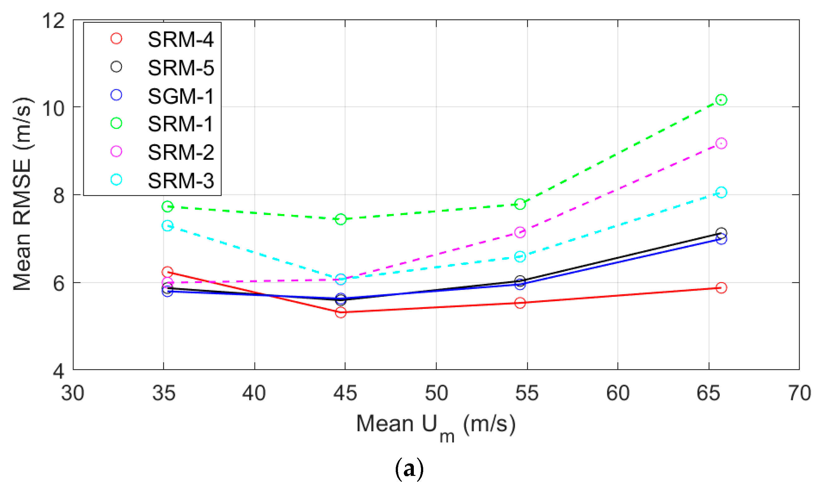
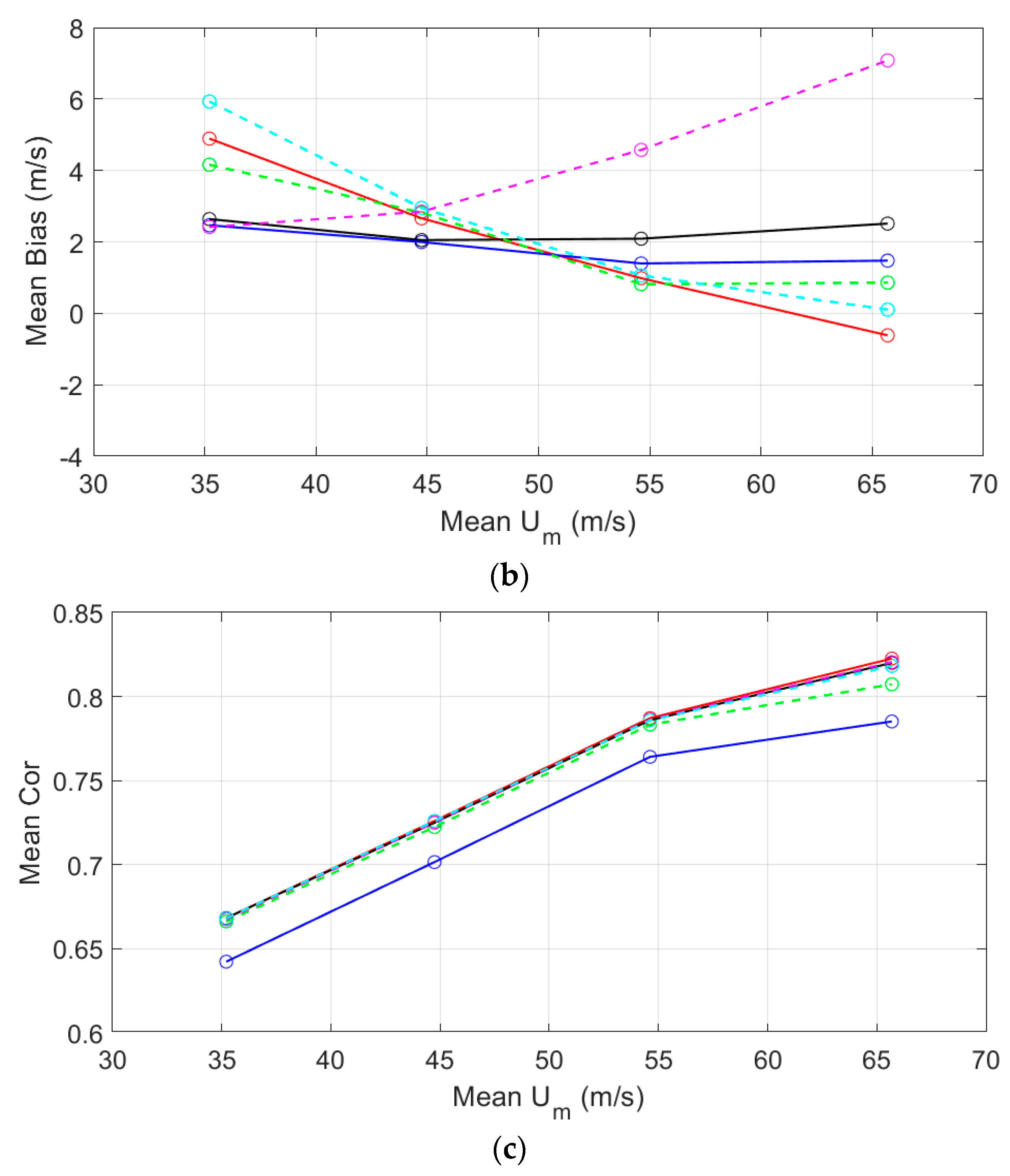
Even though SRMs utilize similar Rankine vortex models as a basis, there are still some differences. According to the mean RMSE values shown in Table 3, the SRMs arranged from good to bad are SRM-4, -5, -3, -2, and -1. The reasons for the accuracy difference include two aspects: methodology and data size.

Firstly, SRM-4 and -5 used Equation (2), but SRM-1, -2, and -3 used Equation (1). The parameter $U_{\mathrm{ma}}$ in Equation (2) makes the models closer to the average wind profiles, leading to a small error.

Secondly, it should be noted that SRM-5 is even better than SRM-3. A possible reason is that the new models utilized 196 TC cases in development, that are much more than 67 TC cases used for SRM-1, -2, and -3.

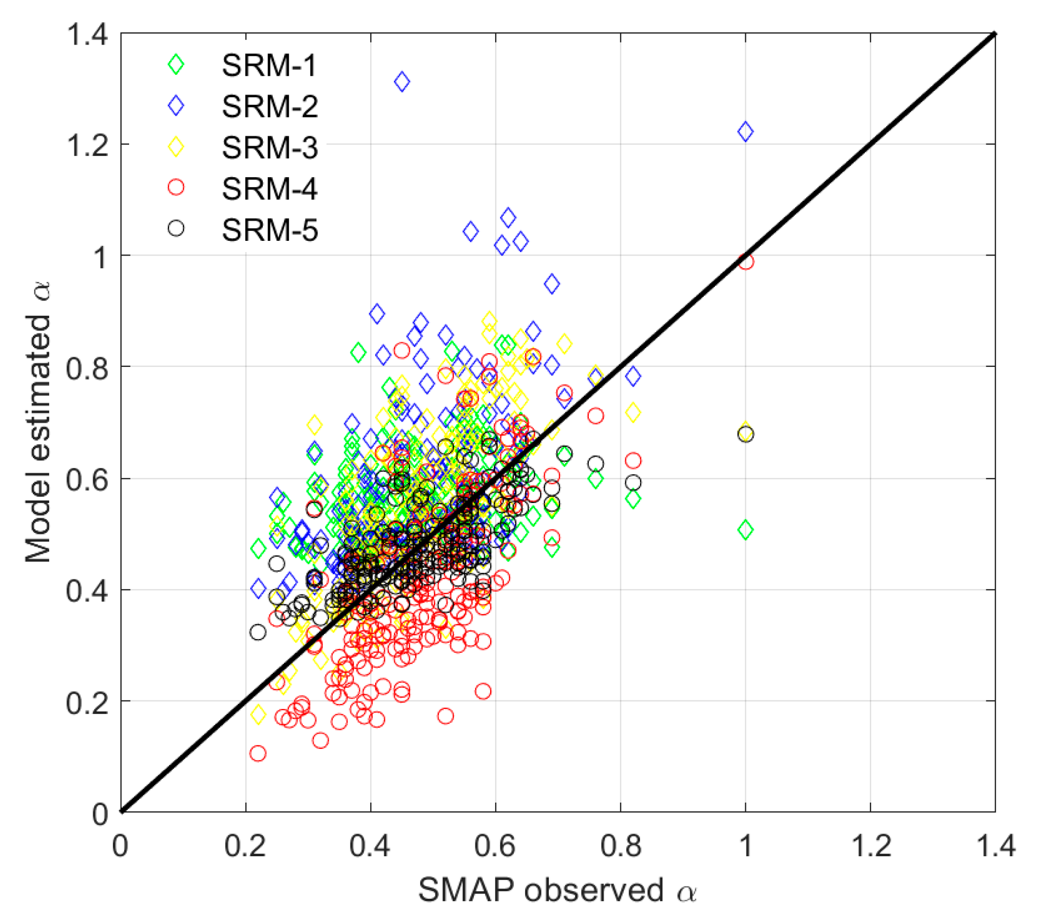
Thirdly, the model’s performance also depends on the accuracy of α parameterization.

Table 5. Different methods of α parameterization in different SRMs.

Model	Method of α Parameterization
SRM-1	$\alpha =0.0091U_{\mathrm{m}}+0.1854$
SRM-2	$\alpha =0.004953R_{\mathrm{m}}+0.3884$
SRM-3	${\alpha =\log }_{{R_{\mathrm{m}}}^{0.78}/93.27\mathrm{}}{\displaystyle \frac{17}{U_{\mathrm{m}}}}$
SRM-4	$\alpha ={\log }_{R_{\mathrm{m}}/(2.408R_{\mathrm{m}}+84.76)}{\displaystyle \frac{17}{U_{\mathrm{ma}}}}$
SRM-5	${\alpha =\mathrm{A}}_1{U_{\mathrm{m}}}^2+{\mathrm{A}}_2{U}_{\mathrm{m}}{R}_{\mathrm{m}}+{\mathrm{A}}_3{R_{\mathrm{m}}}^2+{\mathrm{A}}_4{U}_{\mathrm{m}}+{\mathrm{A}}_5{R}_{\mathrm{m}}+{\mathrm{A}}_6$ 1

¹ A₁–A₆ are listed in Table 1.

shows the α parameterization methods in different SRMs. Figure 9 and

Table 6. Comparison between the α values calculated by SRMs and that fitted from SMAP observations.

Model	RMSE	Bias	Cor
SRM-1	0.15	0.09	0.23
SRM-2	0.17	0.11	0.54
SRM-3	0.13	0.07	0.67
SRM-4	0.13	−0.06	0.70
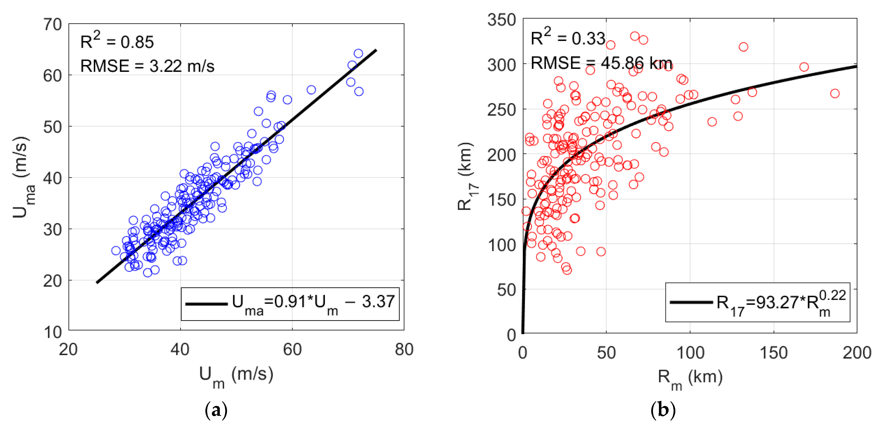
SRM-5	0.08	−2.35 × ${10}^{-5}$	0.70

show the comparison between the model calculated α and the fitted α from SMAP winds. In SRM-3 and -4, the method relates $R_{17}$ and $R_{\mathrm{m}}$ with a strong correlation between them. That can ensure the α parameterization is based on the Rankine vortex, so that SRM-3 and -4 can accurately estimate the radius of 17 m/s. For the other three SRMs, the α parameterizations are fitting α with $U_{\mathrm{m}}$ and $R_{\mathrm{m}}$, separately or together. Among them, quadratic polynomial is better than monomial fitting. 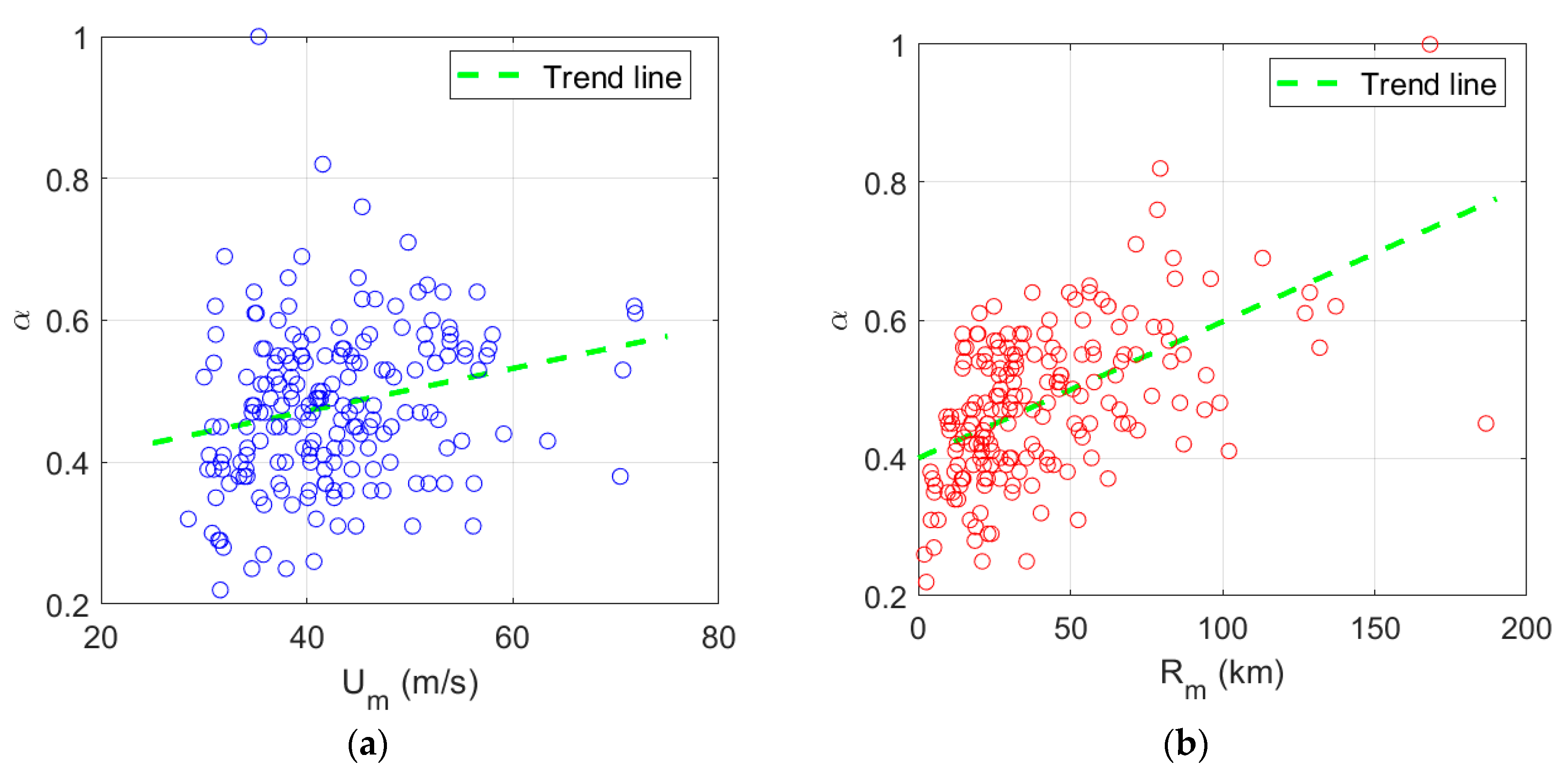In particular, the correlation between α and $U_{\mathrm{m}}$ is not very evident, as shown in Figure 5a, indicating that the SRM-1 has low accuracy. In addition, Figure 9 and Table 6 indicate that the estimation accuracy of α by the SRM-5 model is higher than that of the SRM-4 model. Because the quadratic polynomial method makes the fitting more straightforward.

To summarize, replacing the parameter $U_{\mathrm{m}}$ with $U_{\mathrm{ma}}$, using Rankine vortex or quadratic polynomial for α parameterization and modeling with adequate data can help to improve the accuracy of SRM.

As previously discussed, SRM is a Rankine vortex function and SGM is a Gaussian-like function. We can compare two models, for example, the SRM-5 and the SGM-1, to explain which model is better, because they both used quadratic polynomial for α and $\beta$ parameterization. Table 3 shows that SRM-5 and SGM-1 have similar RMSE, but SGM-1’s bias and Cor is lower. That indicates the systematic bias of SGM-1 is smaller. However, the correlation between the SGM-1 results and actual observations is weaker. In future research, we can investigate whether using a Gaussian-like function for α parameterization can improve the accuracy of this model.

5.2. The Advantages and Limitations of the New Models

Regarding the advantages, both SRM and SGM could estimate TC outer wind profiles only requiring $U_{\mathrm{m}}$ and $R_{\mathrm{m}}$. The models are highly user-friendly. Based on wind profiles, one can get sea surface wind filed accurately.

However, the new models still have some limitations:

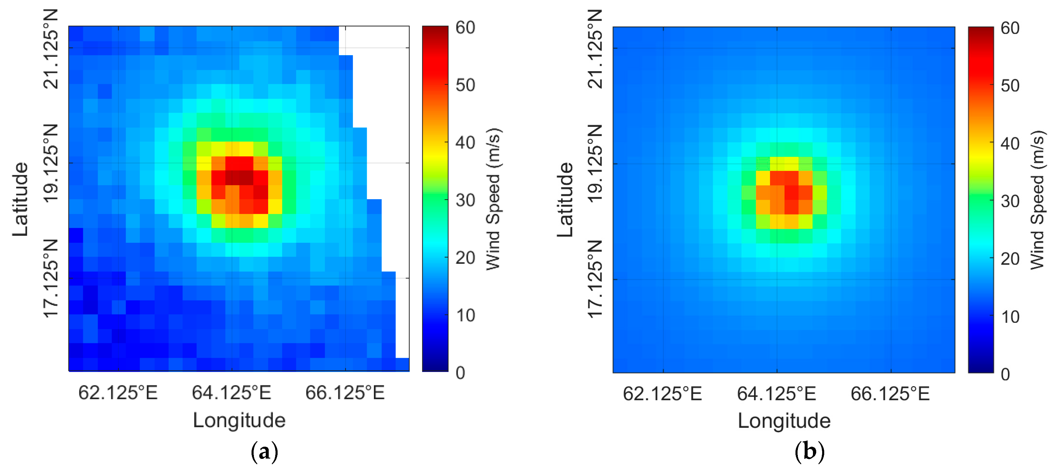
• As shown in Figure 7b–d, the estimated wind fields are circularly symmetrical. This does not reflect the actual conditions in nature and will lead to errors. Although a natural TC wind field always becomes more symmetric when $U_{\mathrm{m}}$ increases, the wind field is not a standard symmetrical shape;
• Although the value of $U_{\mathrm{m}}$ is input into the new models, the estimated profiles cannot reach $U_{\mathrm{m}}$ of the TC. This is because the use of $U_{\mathrm{ma}}$ makes the simulation results closer to the average of the observed data;
• The grid spacing of the modeling data and the validation data is 0.25° × 0.25°. Thus, the new models may have errors if they are used to estimate wind fields with a higher space resolution. This study did not quantitatively assess this issue due to data limitations;
• The proposed models are limited to the outer area, but not the inner core, because the model winds have a large error in the inner core. The error is induced by two issues. Firstly, the used models assume the minimum wind speed is 0 m/s in the inner core. However, it is not 0 m/s for radiometer observations. Secondly, if the model was modified, the first issue can be solved. For example, U = $U_{\mathrm{m}}$R/$R_{\mathrm{m}}$ is converted to U = ($U_{\mathrm{m}}$ − $U_{\mathrm{m}\mathrm{n}}$)R/$R_{\mathrm{m}}$ + $U_{\mathrm{m}\mathrm{n}}$, $U_{\mathrm{m}\mathrm{n}}$ is the minimum wind speed and larger than 0 m/s. However, the spatial resolution of the radiometer observations is just 0.25° × 0.25°, which is too coarse. The locations of the minimum wind points usually do not coincide with the center locations provided by RSS Tropical Cyclones ASCII files. The modified inner core model cannot be used correctly;
• The impact of environmental flow on the results of the TC stationary wind field model is multifaceted, including altering the wind field structure, affecting the cyclone intensity, changing the cyclone track, influencing the cyclone structure, impacting the release of latent heat, and affecting the life cycle of the cyclone. For the proposed models, environmental flow may affect Uma and the symmetry of wind field, affecting the accuracy of the models. Therefore, when using the proposed models, it is helpful to fully consider the influence of environmental flow to improve the accuracy and reliability of the models.

6. Conclusions

This study successfully developed and validated new parametric models for representing the outer radial wind profiles of TCs using SMAP and AMSR-2 satellite data. Based on an extensive analysis of SMAP wind field observation data analysis results, the proposed models, namely SRM-4, SRM-5, and SGM-1, were modified from the Rankine vortex model and the TWP Gaussian model. The following conclusions can be drawn from this study:

• The validation results demonstrate substantial improvements of the proposed models in accuracy compared to existing models. The proposed models offer a more precise depiction of TC wind fields by incorporating key parameters such as maximum wind speed and its radius and average wind speed at the radius of maximum wind;
• The SRM-4 exhibits the best overall performance, with the lowest mean RMSE of 5.57 m/s, maintaining a strong correlation with AMSR-2 observations;
• The SRM-5 demonstrates the highest precision in fitting α from the SMAP observations;
• The models outperform in the Atlantic Ocean, with a Mean RMSE of 5.37 m/s;
• The results indicate that the new models have the potential to enhance the understanding of ocean surface dynamics under TC conditions and improve numerical modeling efforts.

Nevertheless, several limitations remain. The estimated wind fields exhibit circular symmetry, which may not fully capture the asymmetric nature of TCs. Moreover, the models’ reliance on average wind speeds leads to underestimation of peak values. Future research should concentrate on developing models that account for TC asymmetry and incorporate higher-resolution data to improve spatial accuracy. Investigating alternative parameterizations, such as using Gaussian functions for parameter $\beta$ estimation, may also enhance model performance. Additionally, extending the validation to include more diverse TC datasets and comparing the models with other remote sensing techniques could provide a more comprehensive assessment of their applicability. Overall, this study provides an effective approach for future advancements in TC wind field modeling and highlights the importance of leveraging satellite data to improve our understanding of tropical cyclone dynamics.

References

1. Irish, J.L.; Resio, D.T.; Ratcliff, J.J. The Influence of Storm Size on Hurricane Surge. J. Phys. Oceanogr. 2006, 38, 2003–2013. [Google Scholar] [CrossRef]
2. Yu, P.; Johannessen, J.A.; Yan, X.H.; Geng, X.; Zhu, L. A Study of the Intensity of Tropical Cyclone Idai Using Dual-Polarization Sentinel-1 Data. Remote Sens. 2019, 11, 2837. [Google Scholar] [CrossRef]
3. Bai, P.; Wu, L.; Chen, Z.; Xu, J.; Li, B.; Li, P. Investigating the Storm Surge and Flooding in Shenzhen City, China. Remote Sens. 2023, 15, 5002. [Google Scholar] [CrossRef]
4. Zhang, H.; Liu, X.; Wu, R.; Liu, F.; Yu, L.; Shang, X.; Qi, Y.; Wang, Y.; Song, X.; Xie, X.; et al. Ocean Response to Successive Typhoons Sarika and Haima (2016) Based on Data Acquired via Multiple Satellites and Moored Array. Remote Sens. 2019, 11, 2360. [Google Scholar] [CrossRef]
5. Yue, X.; Zhang, B. Effect of Tropical Cyclone Wind Forcing on Improving Upper Ocean Simulation: An Idealized Study. Remote Sens. 2024, 16, 2574. [Google Scholar] [CrossRef]
6. Zhang, W.; Li, R.; Zhu, D.; Zhao, D.; Guan, C. An Investigation of Impacts of Surface Waves-Induced Mixing on the Upper Ocean under Typhoon Megi (2010). Remote Sens. 2023, 15, 1862. [Google Scholar] [CrossRef]
7. Guo, X.; Tan, Z.M. Tropical Cyclone Fullness: A New Concept for Interpreting Storm Intensity. Geophys. Res. Lett. 2017, 44, 4324–4331. [Google Scholar] [CrossRef]
8. Ueno, M.; Bessho, K. A Statistical Analysis of Near-Core Surface Wind Asymmetries in Typhoons Obtained from QuikSCAT Data. J. Meteorol. Soc. Jpn. 2011, 89, 225–241. [Google Scholar] [CrossRef]
9. Holland, G.J.; Belanger, J.I.; Fritz, A. A Revised Model for Radial Profiles of Hurricane Winds. Mon. Weather Rev. 2010, 138, 4393–4401. [Google Scholar] [CrossRef]
10. Xie, L.; Bao, S.; Pietrafesa, L.J.; Foley, K.; Fuentes, M. A Real-Time Hurricane Surface Wind Forecasting Model: Formulation and Verification. Mon. Weather Rev. 2006, 134, 1355–1370. [Google Scholar] [CrossRef]
11. Sun, Z.; Zhang, B.; Zhang, J.A.; Perrie, W. Examination of Surface Wind Asymmetry in Tropical Cyclones over the Northwest Pacific Ocean Using SMAP Observations. Remote Sens. 2019, 11, 2604. [Google Scholar] [CrossRef]
12. Mallen, K.J.; Montgomery, M.T.; Wang, B. Reexamining the Near-Core Radial Structure of the Tropical Cyclone Primary Circulation: Implications for Vortex Resiliency. J. Atmos. Sci. 2005, 62, 408–425. [Google Scholar] [CrossRef]
13. Holland, G.J. An Analytic Model of the Wind and Pressure Profiles in Hurricanes. Mon. Weather Rev. 1980, 108, 1212–1218. [Google Scholar] [CrossRef]
14. Krien, Y.; Arnaud, G.; Cécé, R.; Ruf, C.; Belmadani, A.; Khan, J.; Bernard, D.; Islam, A.K.M.S.; Durand, F.; Testut, L.; et al. Can We Improve Parametric Cyclonic Wind Fields Using Recent Satellite Remote Sensing Data? Remote Sens. 2018, 10, 1963. [Google Scholar] [CrossRef]
15. Zhang, G.; Perrie, W.; Zhang, B.; Yang, J.; He, Y. Monitoring of tropical cyclone structures in ten years of RADARSAT-2 SAR images. Remote Sens. Environ. 2020, 236, 111449. [Google Scholar] [CrossRef]
16. Zhang, G.; Zhang, B.; Perrie, W.; Xu, Q.; He, Y. A Hurricane Tangential Wind Profile Estimation Method for C-Band Cross-Polarization SAR. IEEE Trans. Geosci. Remote Sens. 2014, 52, 7186–7194. [Google Scholar] [CrossRef]
17. Wang, S.; Yang, X.; Portabella, M.; Yuen, K.-V.; Zhang, M.; Du, Y. A SAR-Based Parametric Model for Tropical Cyclone Tangential Wind Speed Estimation. IEEE J. Sel. Top. Appl. Earth Obs. Remote Sens. 2022, 15, 8806–8818. [Google Scholar] [CrossRef]
18. Wood, V.T.; White, L.W. A New Parametric Model of Vortex Tangential-Wind Profiles: Development, Testing, and Verification. J. Atmos. Sci. 2011, 68, 990–1006. [Google Scholar] [CrossRef]
19. Mouche, A.; Chapron, B.; Knaff, J.; Zhao, Y.; Zhang, B.; Combot, C. Copolarized and Cross-Polarized SAR Measurements for High-Resolution Description of Major Hurricane Wind Structures: Application to Irma Category 5 Hurricane. J. Geophys. Res. Oceans 2019, 124, 3905–3922. [Google Scholar] [CrossRef]
20. Gao, Y.; Wang, Y.; Wang, W. A New Approach for Ocean Surface Wind Speed Retrieval Using Sentinel-1 Dual-Polarized Imagery. Remote Sens. 2023, 15, 4267. [Google Scholar] [CrossRef]
21. Meissner, T.; Wentz, F. The Emissivity of the Ocean Surface Between 6 and 90 GHz Over a Large Range of Wind Speeds and Earth Incidence Angles. IEEE Trans. Geosci. Remote Sens. 2012, 50, 3004–3026. [Google Scholar] [CrossRef]
22. Reul, N.; Tenerelli, J.; Chapron, B.; Vandemark, D.; Quilfen, Y.; Kerr, Y. SMOS satellite L-band radiometer: A new capability for ocean surface remote sensing in hurricanes. J. Geophys. Res. Oceans 2012, 117, C02006. [Google Scholar] [CrossRef]
23. Sharma, N. A new approach for estimating ocean-surface wind speed using an SMAP L-band radiometer. Weather 2018, 74, S7–S12. [Google Scholar] [CrossRef]
24. Fore, A.G.; Yueh, S.H.; Stiles, B.W.; Tang, W.; Hayashi, A.K. SMAP Radiometer-Only Tropical Cyclone Intensity and Size Validation. IEEE Geosci. Remote Sens. Lett. 2018, 15, 1480–1484. [Google Scholar] [CrossRef]
25. Meissner, T.; Ricciardulli, L.; Wentz, F.J. Capability of the SMAP Mission to Measure Ocean Surface Winds in Storms. Bull. Amer. Meteor. Soc. 2017, 98, 1660–1677. [Google Scholar] [CrossRef]
26. Reul, N.; Chapron, B.; Zabolotskikh, E.; Donlon, C.; Quilfen, Y.; Guimbard, S.; Piolle, J.F. A revised L-band radio-brightness sensitivity to extreme winds under Tropical Cyclones: The five year SMOS-storm database. Remote Sens. Environ. 2016, 180, 274–291. [Google Scholar] [CrossRef]
27. Shao, W.; Lai, Z.; Nunziata, F.; Buono, A.; Jiang, X.; Zuo, J. Wind Field Retrieval with Rain Correction from Dual-Polarized Sentinel-1 SAR Imagery Collected during Tropical Cyclones. Remote Sens. 2022, 14, 5006. [Google Scholar] [CrossRef]
28. Won Jeong, P.; Korosov, A.; Babiker, M.; Sandven, S.; Won, J.-S. Efficient Thermal Noise Removal for Sentinel-1 TOPSAR Cross-Polarization Channel. IEEE Trans. Geosci. Remote Sens. 2017, 56, 1555–1565. [Google Scholar]
29. Wang, S.; Yang, X.; Li, H.; Ren, K.; Yin, X.; Hu, D.; Du, Y. An Improved Asymmetric Hurricane Parametric Model Based on Cross-Polarization SAR Observations. IEEE J. Sel. Topics Appl. Earth Observ. Remote Sens. 2020, 14, 1411–1422. [Google Scholar] [CrossRef]
30. Zhang, G.; Li, X.; Perrie, W.; Zhang, J. Tropical Cyclone Winds and Inflow Angle Asymmetry from SAR Imagery. Geophys. Res. Lett. 2021, 48, e2021GL095699. [Google Scholar] [CrossRef]
31. Zhang, G.; Perrie, W.; Li, X.; Zhang, J.A. A Hurricane Morphology and Sea Surface Wind Vector Estimation Model Based on C-Band Cross-Polarization SAR Imagery. IEEE Trans. Geosci. Remote Sens. 2017, 55, 1743–1751. [Google Scholar] [CrossRef]
32. Gao, Y.; Zhang, J.; Guan, C.; Sun, J. Analyzing Sea Surface Wind Distribution Characteristics of Tropical Cyclone Based on Sentinel-1 SAR Images. Remote Sens. 2021, 13, 4501. [Google Scholar] [CrossRef]
33. Gao, Y.; Zhang, J.; Sun, J.; Guan, C. Application of SAR Data for Tropical Cyclone Intensity Parameters Retrieval and Symmetric Wind Field Model Development. Remote Sens. 2021, 13, 2902. [Google Scholar] [CrossRef]
34. Gao, Y.; Sun, J.; Guan, C.; Wang, Y. New Rankine Vortex Models Developed Based on SMAP Measurements. J. Atmos. Ocean. Technol. 2024, 41, 1017–1027. [Google Scholar] [CrossRef]
35. Mouche, A.A.; Chapron, B.; Zhang, B.; Husson, R. Combined Co- and Cross-Polarized SAR Measurements Under Extreme Wind Conditions. IEEE Trans. Geosci. Remote Sens. 2017, 55, 6746–6755. [Google Scholar] [CrossRef]
36. Zhang, G.; Xu, C.; Li, X.; Zhu, Z.; Perrie, W. Tropical Cyclone Center and Symmetric Structure Estimating From SMAP Data. IEEE Trans. Geosci. Remote Sens. 2022, 60, 4205311. [Google Scholar] [CrossRef]
37. Kumar, P.; Gairola, R. Fostering the Need of L-Band Radiometer for Extreme Oceanic Wind Research. IEEE Trans. Geosci. Remote Sens. 2021, 60, 4103906. [Google Scholar] [CrossRef]
38. Manaster, A.; Ricciardulli, L.; Meissner, T. Tropical Cyclone Winds from WindSat, AMSR2, and SMAP: Comparison with the HWRF Model. Remote Sens. 2021, 13, 2347. [Google Scholar] [CrossRef]
39. Wentz, F.J.; Meissner, T.; Gentemann, C.; Hilburn, K.A.; Scott, J. RSS GCOM-W1 AMSR2 Daily Environmental Suite on 0.25 deg grid, Version 8.2; Remote Sensing Systems: Santa Rosa, CA, USA, 2021. [Google Scholar]
Figure 1. Flowchart of this study.
Remotesensing 17 01564 g001
Figure 2. The TC sample information in the SMAP modeling dataset: (a) the locations and categories (Saffir–Simpson hurricane wind scale: Tropical Storm: 18–32 m/s; Category 1: 33–42 m/s; Category 2: 43–49 m/s; Category 3: 49–57 m/s; Category 4: 58–70 m/s; and Category 5: ≥70 m/s); (b) sample numbers in different categories; and (c) sample numbers in different years and ocean basins. There are 196 TC samples over the Atlantic Ocean (AL), the Central Pacific (CP), the East Pacific Ocean (EP), the Indian Ocean (IO), the Southern Hemisphere Ocean (SH), and the West Pacific Ocean (WP).
Remotesensing 17 01564 g002aRemotesensing 17 01564 g002b
Figure 3. The TC sample information in the AMSR-2 validation dataset: (a) the locations and categories (Saffir–Simpson hurricane wind scale: Tropical Storm: 18–32 m/s; Category 1: 33–42 m/s; Category 2: 43–49 m/s; Category 3: 49–57 m/s; Category 4: 58–70 m/s; and Category 5: ≥70 m/s); (b) sample numbers in different categories; and (c) sample numbers in different years and ocean basins. There are 126 TC samples over the Atlantic Ocean (AL), the Central Pacific (CP), the East Pacific Ocean (EP), the Indian Ocean (IO), the Southern Hemisphere Ocean (SH), and the West Pacific Ocean (WP).
Remotesensing 17 01564 g003
Figure 4. (a) The comparison between U ma and U m (blue circles); (b) the comparison between R 17 and R m (red circles). In (a,b), the black curves stand for fitting functions.
Remotesensing 17 01564 g004
Figure 5. The comparisons between α and (a) U m (blue circles) and (b) R m (red circles). The green dashed lines stand for trends.
Remotesensing 17 01564 g005
Figure 6. The comparisons between β and (a) U m (blue circles) and (b) R m (red circles). The green dashed lines stand for trends.
Remotesensing 17 01564 g006
Figure 7. A case study of the sea surface wind fields for Tropical Cyclone Kyarr. (a) the SMAP observations on 13:42 UTC 28 October 2019; (b) the corresponding wind field calculated with SRM-4; (c) the corresponding wind field calculated with SRM-5; (d) the corresponding wind field calculated with SGM-1; and (e) the outer wind profiles from the three models and the SMAP wind data.
Remotesensing 17 01564 g007aRemotesensing 17 01564 g007b
Figure 8. Validations of the model-estimated wind speeds with the AMSR-2 observations. The statistics of (a) mean RMSE; (b) mean bias; and (c) mean Cor are compared with Mean U m in four groups: 30   m / s U m < 40   m / s , 40   m / s U m < 50   m / s , 50   m / s U m < 60   m / s , and 60   m / s U m . Solid lines are the proposed models. Dashed lines are the existing models.
Remotesensing 17 01564 g008aRemotesensing 17 01564 g008b
Figure 9. Model calculated α vs. fitted α from SMAP observations.
Remotesensing 17 01564 g009