1. Introduction
Tropical cyclones (TC) are a destructive weather system, causing strong wind, huge waves, intense rainfall, and storm surges [
1,
2,
3]. TC ocean surface wind fields are relevant to several oceanic and atmospheric variables, such as heat, moisture, and momentum fluxes, which are important driving factors for atmospheric numerical models to guide TC evolution forecasting and risk assessment [
4,
5,
6]. Thus, it is a key research area to investigate the characteristics of TC wind field and the methodology to estimate them in the aspects of intensity, size, structure, and distribution [
7,
8,
9,
10,
11].
In the TC system, along the radial direction, the ocean surface wind speeds increase from central minimum to eyewall maximum and then decay with an increasing radius (
R). The radial wind profile is a useful tool to describe this variation [
12,
13]. The parametric representation of wind profiles is an active area of research [
14]. With the improvement in numerical simulation and the accumulation of observations, more and more parametric models have been established to compute wind profiles, such as the Holland hurricane model, the tangential wind profile (TWP) Gaussian model, the Gauss vortex model, the Rankine vortex model, and their modified versions [
12,
15,
16,
17,
18]. Their advantage is that one can construct the entire wind field simply with limited observations, such as maximum wind speed (
) and its radius (
). Moreover, by adjusting the decay exponent (α), the modified Rankine vortex model has better performance than the pure Rankine vortex model, because different TC intensities correspond to different decay exponents.
With the development of remote sensing techniques, spaceborne active and passive microwave radars have been employed day and night to monitor TC systems with a large swath. For example, synthetic aperture radar (SAR) with a cross-polarization mode can retrieve wind speeds up to about 70 m/s at a high spatial resolution [
19,
20]. The L-band radiometers, such as the Soil Moisture Active Passive (SMAP) and the Soil Moisture and Ocean Salinity (SMOS), can also measure wind speeds in intense tropical and extratropical storms [
21,
22,
23,
24]. Its spatial resolution is not as high as SAR; however, the signal is not affected by rainfall and thermal noise [
25,
26,
27,
28].
Up to now, abundant satellite observations have become new data sources for modifying TC parametric wind filed models [
29,
30]. For example, based on 16 RADARSAT-2 Scan-SAR images, the Symmetric Hurricane Estimates for Wind (SHEW) model was developed by combining the Rankine vortex model and the reference ellipse [
31]. The radial distributions were within 150 km from the hurricane centers. By fitting this model to the SAR retrieved wind field, one can derive five TC morphology parameters: ellipse major axis, ellipse minor axis,
,
and
α of the Rankine vortex, and then use them to estimate hurricane wind directions with the inflow angle model. Based on 11 Sentinel-1 images, Wang et al. proposed the TWP model, as a piecewise Gaussian-like function [
17]. The model parameters
a and
b (we named it
in our new model), corresponding to
R ≤
and
<
R < 150 km, were fitted with the azimuth-averaged wind speeds. In their work,
a and
b were related to three TC intensity categories: the Small (
< 33.1 m/s), the Moderate (33.1 m/s ≤
< 49.2 m/s), and the Major (
≥ 49.2 m/s). However, for these categories, the corresponding mean
b values were 0.99, 1.01, and 0.93, respectively, which were not dependent on intensity categories. In addition, the relationship between
b and
was ambiguous for the collected profiles in the Small and Moderate categories. This implies that the TWP model may have large errors when estimating TC outer (
R ) wind field just with
and
. In summary, when using the SHEW model and the TWP model to estimate TC wind fields, both need initial entire observed wind fields to fit
α,
a, and
b. This raises the question: since wind fields have been observed, why does one estimate them again?
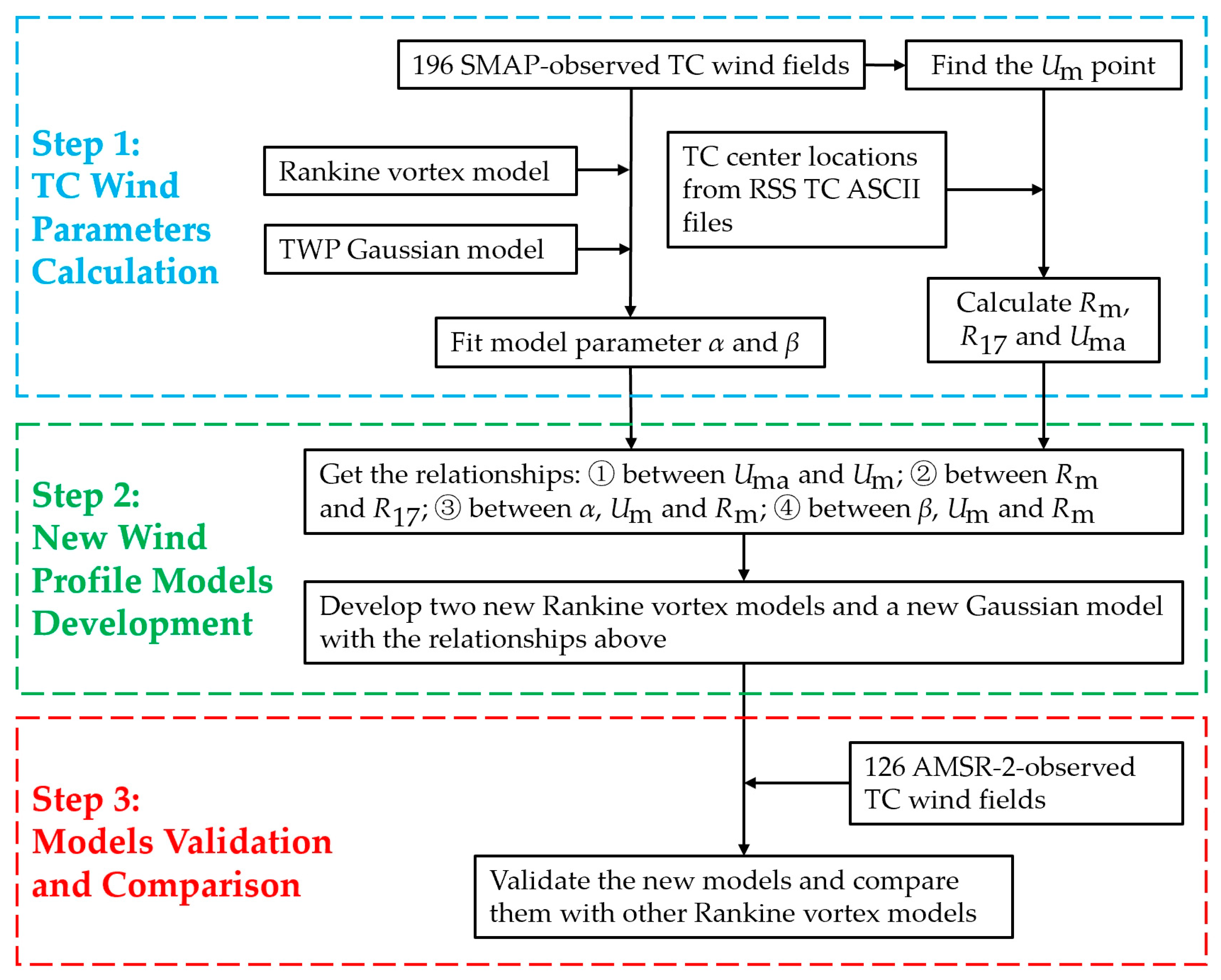
To solve this problem above, we had proposed SAR-data-based and SMAP-data-based Rankine vortex models by establishing empirical functions between
α,
, and
[
32,
33,
34]. The Rankine model for outer wind field is
. The models can estimate TC outer wind profile, if
and
are known. However, the modeling process still has two problems. Firstly,
α values were calculated from 17 m/s,
(the average radius of 17 m/s),
, and
, instead of being fitted from initial wind fields. This indicates that
α can only stand for the wind decay for the
point and the 17 m/s point, instead of whole wind field. Secondly, the three models cannot provide average wind variation near the
point, leading to definite overestimations. Because when
R =
, the models make all points
.
is the maximum but not the average. In fact, the TC wind field is asymmetric. When
R =
, there are many points with
. This paper seeks to address the above two problems to parametrically represent TC wind profile more accurately.
5. Discussion
According to the validation and comparison, this section discusses the differences, advantages, and limitations of the six models (SRM-1, -2, -3, -4, -5, and SGM-1), and the reasons.
5.1. The Model Differences
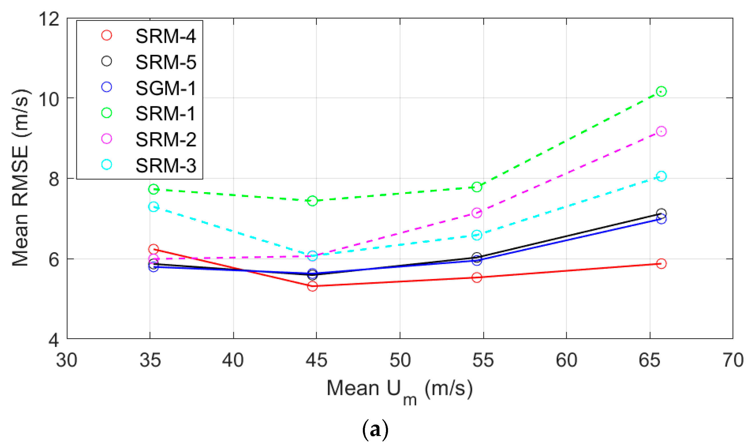
Even though SRMs utilize similar Rankine vortex models as a basis, there are still some differences. According to the mean RMSE values shown in
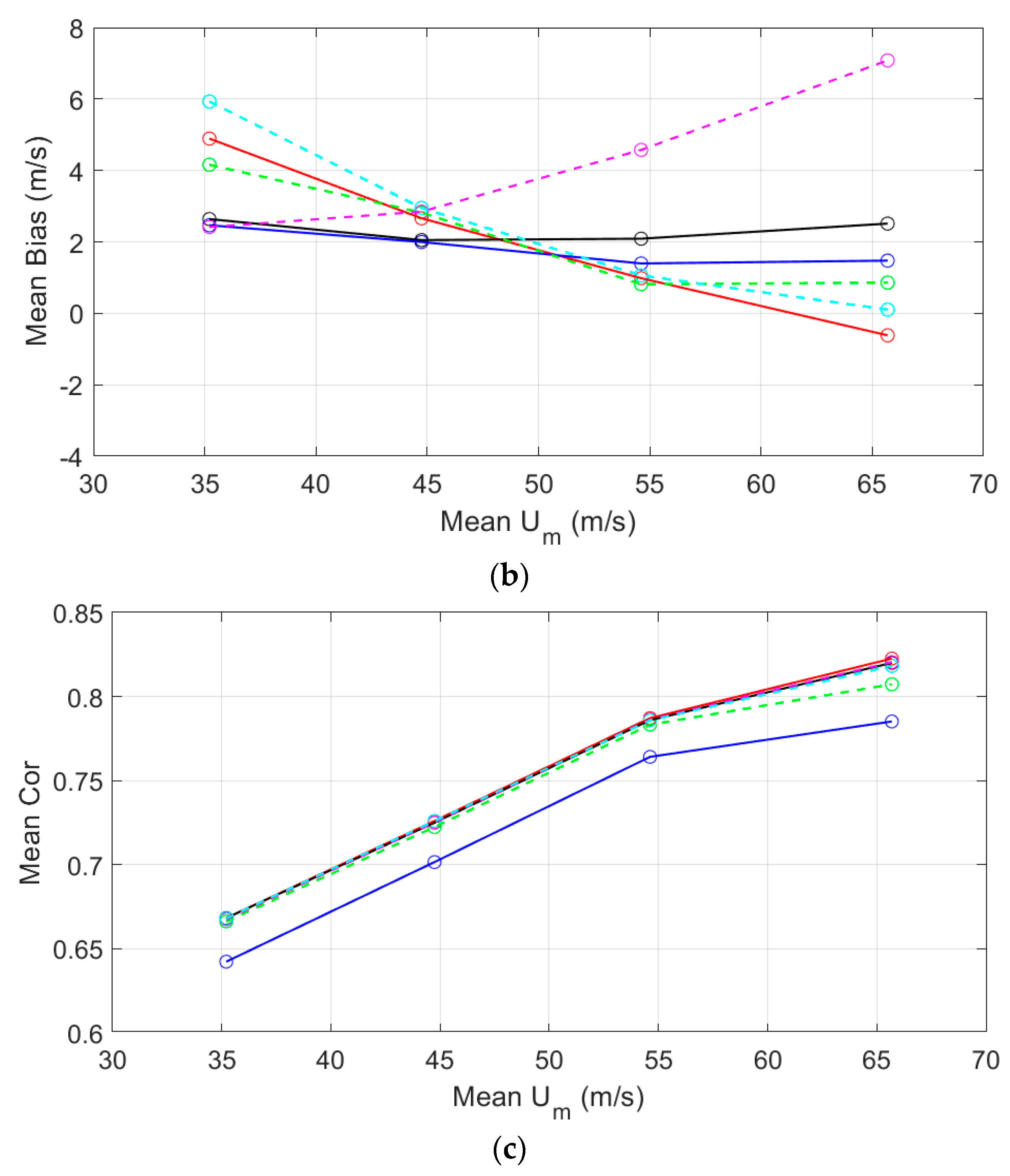
Table 3, the SRMs arranged from good to bad are SRM-4, -5, -3, -2, and -1. The reasons for the accuracy difference include two aspects: methodology and data size.
Firstly, SRM-4 and -5 used Equation (2), but SRM-1, -2, and -3 used Equation (1). The parameter in Equation (2) makes the models closer to the average wind profiles, leading to a small error.
Secondly, it should be noted that SRM-5 is even better than SRM-3. A possible reason is that the new models utilized 196 TC cases in development, that are much more than 67 TC cases used for SRM-1, -2, and -3.
Thirdly, the model’s performance also depends on the accuracy of
α parameterization.
Table 5 shows the α parameterization methods in different SRMs.
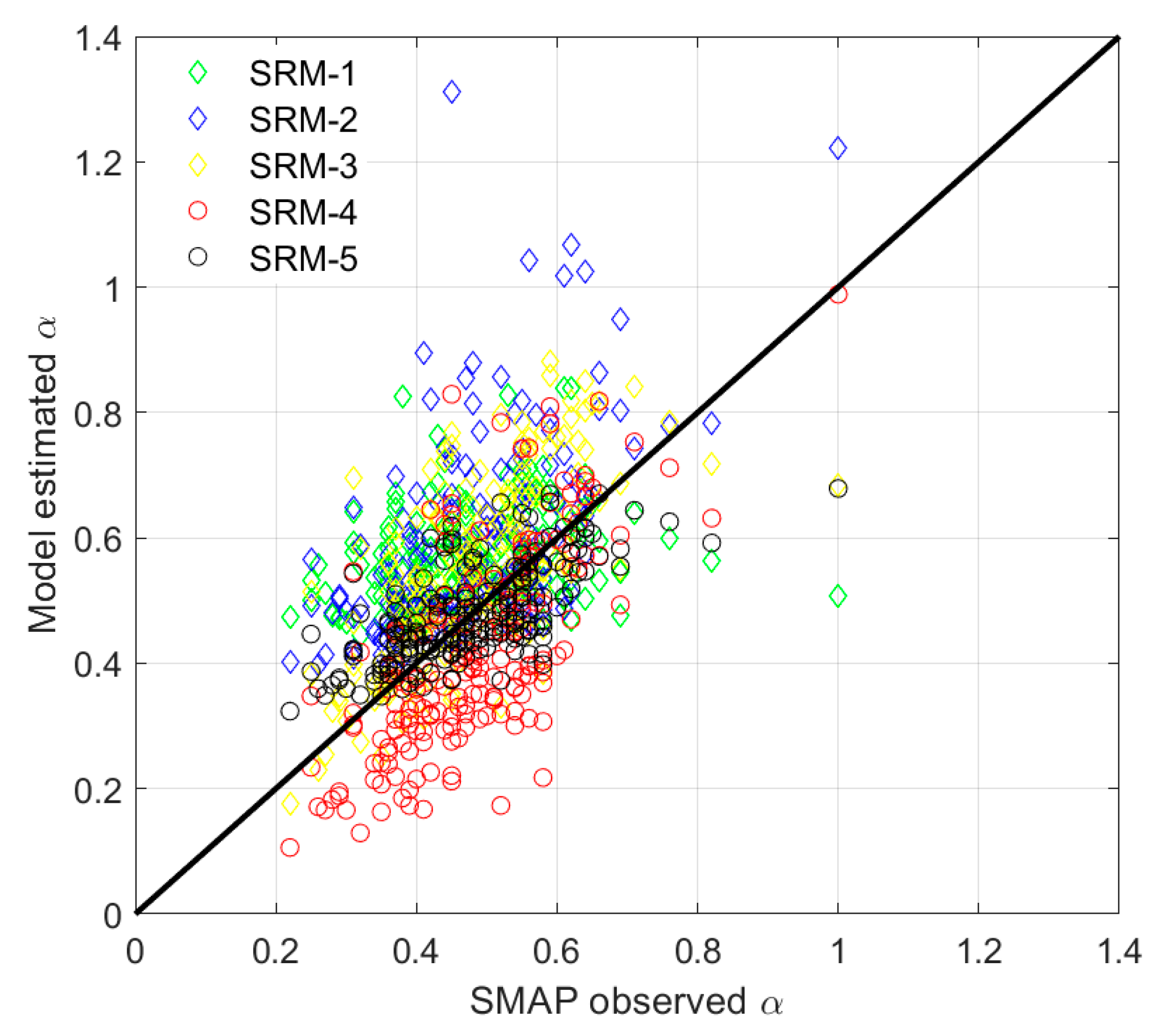
Figure 9 and
Table 6 show the comparison between the model calculated α and the fitted α from SMAP winds. In SRM-3 and -4, the method relates
and
with a strong correlation between them. That can ensure the
α parameterization is based on the Rankine vortex, so that SRM-3 and -4 can accurately estimate the radius of 17 m/s. For the other three SRMs, the α parameterizations are fitting α with
and
, separately or together. Among them, quadratic polynomial is better than monomial fitting. In particular, the correlation between
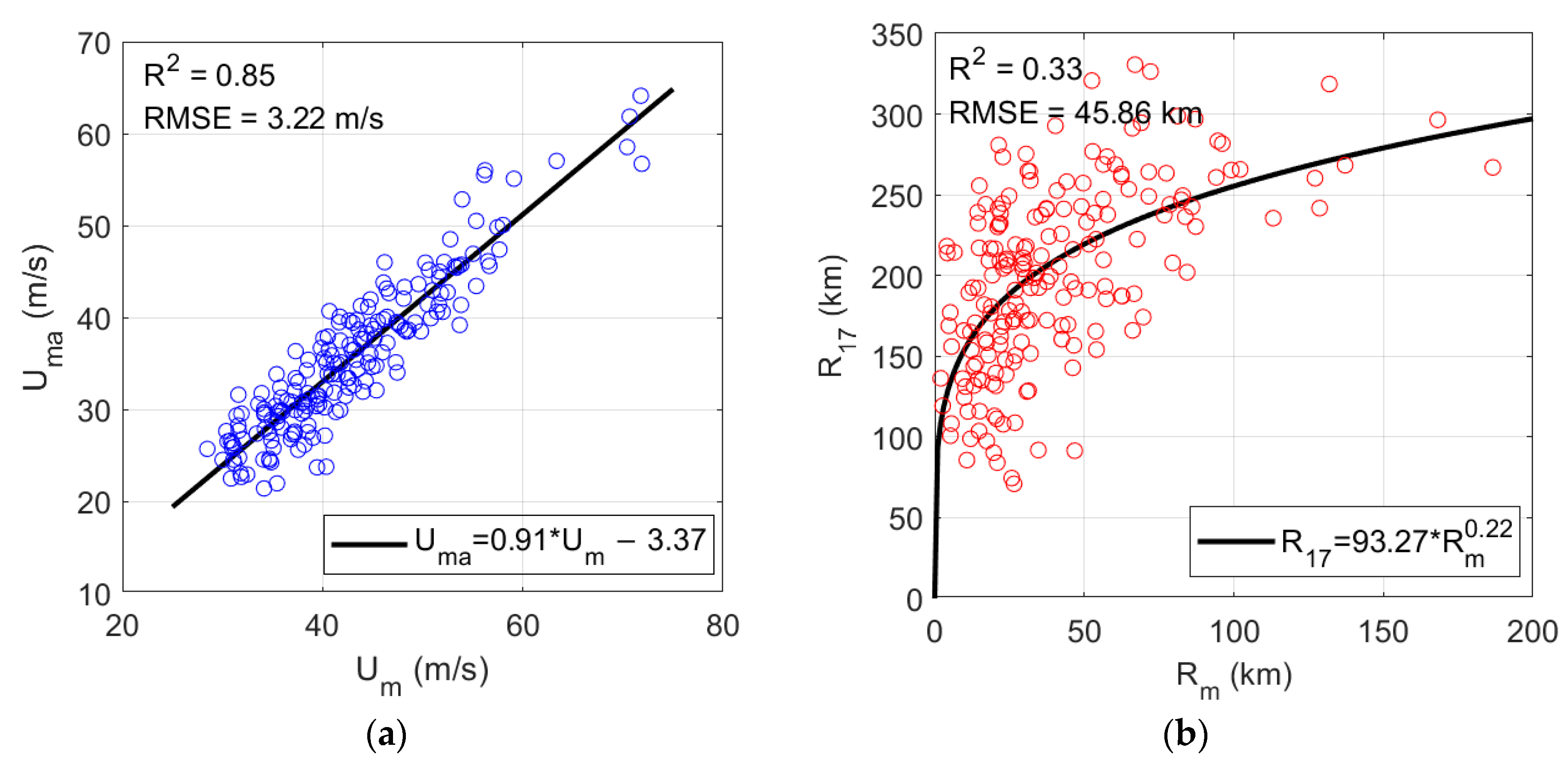
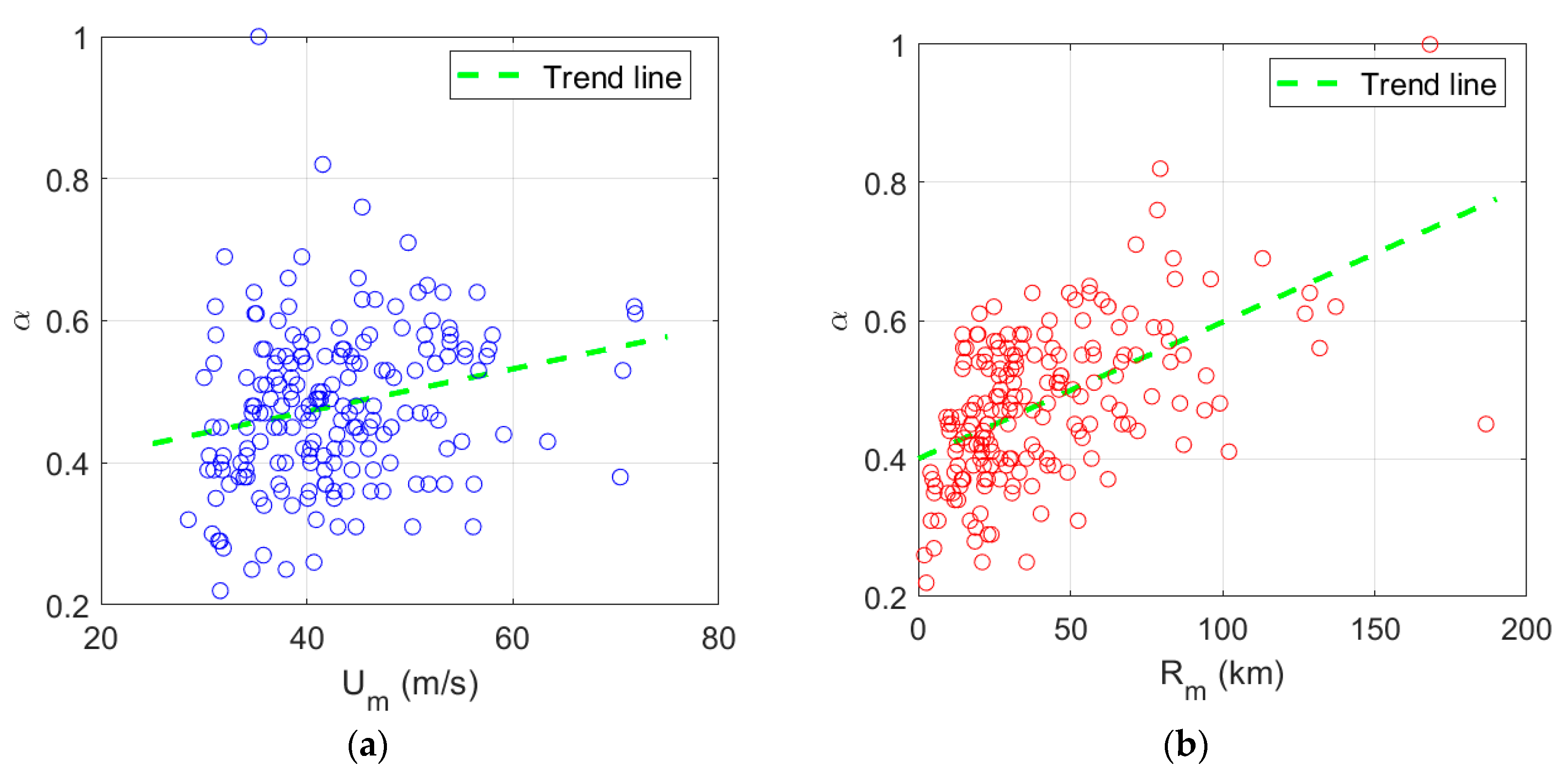
α and
is not very evident, as shown in
Figure 5a, indicating that the SRM-1 has low accuracy. In addition,
Figure 9 and
Table 6 indicate that the estimation accuracy of α by the SRM-5 model is higher than that of the SRM-4 model. Because the quadratic polynomial method makes the fitting more straightforward.
To summarize, replacing the parameter with , using Rankine vortex or quadratic polynomial for α parameterization and modeling with adequate data can help to improve the accuracy of SRM.
As previously discussed, SRM is a Rankine vortex function and SGM is a Gaussian-like function. We can compare two models, for example, the SRM-5 and the SGM-1, to explain which model is better, because they both used quadratic polynomial for
α and
parameterization.
Table 3 shows that SRM-5 and SGM-1 have similar RMSE, but SGM-1’s bias and Cor is lower. That indicates the systematic bias of SGM-1 is smaller. However, the correlation between the SGM-1 results and actual observations is weaker. In future research, we can investigate whether using a Gaussian-like function for
α parameterization can improve the accuracy of this model.
5.2. The Advantages and Limitations of the New Models
Regarding the advantages, both SRM and SGM could estimate TC outer wind profiles only requiring and . The models are highly user-friendly. Based on wind profiles, one can get sea surface wind filed accurately.
However, the new models still have some limitations:
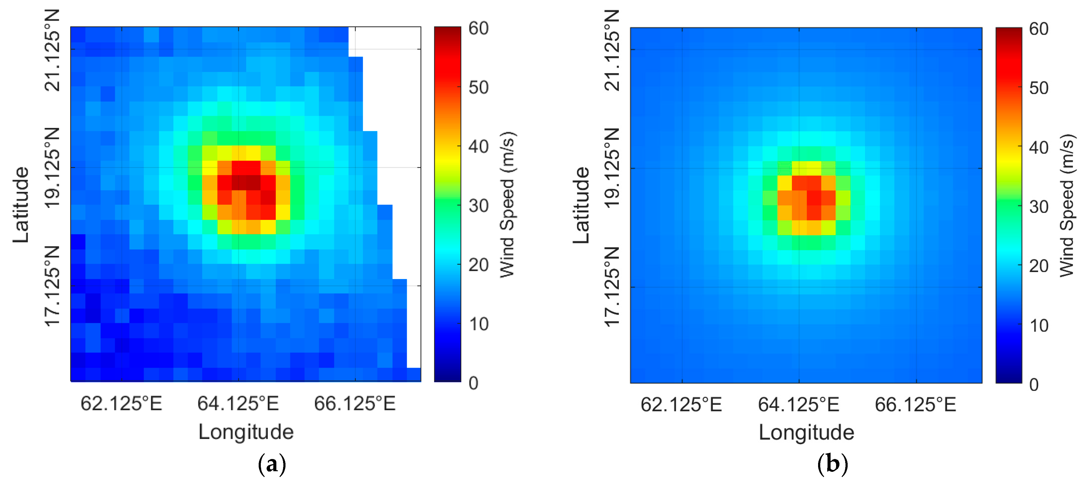
As shown in
Figure 7b–d, the estimated wind fields are circularly symmetrical. This does not reflect the actual conditions in nature and will lead to errors. Although a natural TC wind field always becomes more symmetric when
increases, the wind field is not a standard symmetrical shape;
Although the value of is input into the new models, the estimated profiles cannot reach of the TC. This is because the use of makes the simulation results closer to the average of the observed data;
The grid spacing of the modeling data and the validation data is 0.25° × 0.25°. Thus, the new models may have errors if they are used to estimate wind fields with a higher space resolution. This study did not quantitatively assess this issue due to data limitations;
The proposed models are limited to the outer area, but not the inner core, because the model winds have a large error in the inner core. The error is induced by two issues. Firstly, the used models assume the minimum wind speed is 0 m/s in the inner core. However, it is not 0 m/s for radiometer observations. Secondly, if the model was modified, the first issue can be solved. For example, U = R/ is converted to U = ( − )R/ + , is the minimum wind speed and larger than 0 m/s. However, the spatial resolution of the radiometer observations is just 0.25° × 0.25°, which is too coarse. The locations of the minimum wind points usually do not coincide with the center locations provided by RSS Tropical Cyclones ASCII files. The modified inner core model cannot be used correctly;
The impact of environmental flow on the results of the TC stationary wind field model is multifaceted, including altering the wind field structure, affecting the cyclone intensity, changing the cyclone track, influencing the cyclone structure, impacting the release of latent heat, and affecting the life cycle of the cyclone. For the proposed models, environmental flow may affect Uma and the symmetry of wind field, affecting the accuracy of the models. Therefore, when using the proposed models, it is helpful to fully consider the influence of environmental flow to improve the accuracy and reliability of the models.
6. Conclusions
This study successfully developed and validated new parametric models for representing the outer radial wind profiles of TCs using SMAP and AMSR-2 satellite data. Based on an extensive analysis of SMAP wind field observation data analysis results, the proposed models, namely SRM-4, SRM-5, and SGM-1, were modified from the Rankine vortex model and the TWP Gaussian model. The following conclusions can be drawn from this study:
The validation results demonstrate substantial improvements of the proposed models in accuracy compared to existing models. The proposed models offer a more precise depiction of TC wind fields by incorporating key parameters such as maximum wind speed and its radius and average wind speed at the radius of maximum wind;
The SRM-4 exhibits the best overall performance, with the lowest mean RMSE of 5.57 m/s, maintaining a strong correlation with AMSR-2 observations;
The SRM-5 demonstrates the highest precision in fitting α from the SMAP observations;
The models outperform in the Atlantic Ocean, with a Mean RMSE of 5.37 m/s;
The results indicate that the new models have the potential to enhance the understanding of ocean surface dynamics under TC conditions and improve numerical modeling efforts.
Nevertheless, several limitations remain. The estimated wind fields exhibit circular symmetry, which may not fully capture the asymmetric nature of TCs. Moreover, the models’ reliance on average wind speeds leads to underestimation of peak values. Future research should concentrate on developing models that account for TC asymmetry and incorporate higher-resolution data to improve spatial accuracy. Investigating alternative parameterizations, such as using Gaussian functions for parameter estimation, may also enhance model performance. Additionally, extending the validation to include more diverse TC datasets and comparing the models with other remote sensing techniques could provide a more comprehensive assessment of their applicability. Overall, this study provides an effective approach for future advancements in TC wind field modeling and highlights the importance of leveraging satellite data to improve our understanding of tropical cyclone dynamics.
