Abstract
This paper describes the benefits of using a microwave radiative transfer model (RTM) to improve the inter-satellite radiometric calibration (XCAL) between two independent satellite microwave radiometers. Because this work was sponsored by the NASA Global Precipitation Mission, the emphasis of this paper is on radiometer channels that are used for atmospheric precipitation retrievals; however, this technique is applicable for microwave remote sensing in general, over a wide range of satellite remote-sensing applications. An XCAL example is presented for the NASA Global Precipitation Mission, whereby the GPM Microwave Imager is used to calibrate another microwave radiometer (TROPICS) within the GPM constellation of satellites. This approach involves intercomparing near-simultaneous measured brightness temperatures from these radiometers viewing a common homogeneous ocean scene. The double difference between observed and theoretical brightness temperature, derived using a radiative transfer model, is used to establish a radiometric calibration offset or bias. On-orbit comparisons are presented for two different approaches, namely, with and without the aid of the RTM. The results demonstrate significant improvements in the XCAL biases derived when using the RTM, and this is especially beneficial when one radiometer produces anomalous brightness temperatures.
1. Introduction
Microwave remote sensing of the earth is challenging because it involves the absolute measurement of earth emission radiance intensity (brightness temperature, Tb) to a precision of order 1 K and an accuracy (bias) of a few Kelvins. Further, the retrieval of environmental parameters involves the simultaneous solution of multispectral Tb observations, therefore most satellite radiometers have multiple channels operating at widely separated frequencies. Because of this, the intra-channel and the inter-satellite radiometric calibration of the passive microwave radiometers (PMRs) is an important issue.
Concerning the pre-launch intra-channel radiometric calibration, the microwave remote sensing community follows the successful infrared community in using blackbody targets for the receiver and detector absolute calibration. However, for microwaves, the optics (antennas) are a much greater challenge because of their inferior collection efficiencies. For example, for microwave remote sensing, the standard is typically 90%, which is augmented with signal processing corrections (sidelobes and cross-polarization mixing) to approach a >95% goal. On the other hand, once launched into space, microwave radiometers have been observed to be very stable, which facilitates their on-orbit calibration. However, the inter-satellite radiometric calibration between radiometers of different designs is considerably more difficult because both the radiometer design parameters and orbital geometry affect the measured scene radiance for a given set of environmental parameters of the atmosphere and surface.
In this paper, we discuss these issues and present a brief history of on-orbit inter-satellite radiometric calibration (XCAL). This is followed by the presentation of our double difference technique for XCAL, which employs a radiative transfer model (RTM). Next, empirical results are presented for XCAL between two satellite microwave radiometers, namely, the Global Precipitation Measurement (GPM) Microwave Imager (GMI) and the Time-Resolved Observations of Precipitation structure and storm Intensity with a Constellation of Small satellites mission (TROPICS). The dataset provided for GMI and TROPICS is in 1base file format, which is a specialized form of the 1B dataset provided by NASA, which includes the radiometric calibrated brightness temperatures, geolocation parameters, and noise-equivalent spectral radiance data (NESR). These inter-satellite comparisons demonstrate the significant advantage of using the double difference of measured and theoretical Tb derived from a radiative transfer model. Finally, we conclude the paper with a discussion of future research in this important area.
1.1. Satellite XCAL History
As presented by Biswas et al. [1], the history of inter-satellite radiometric calibration for microwave imagers began with the launch of the first Special Sensor Microwave Imager (SSMI) on the DMSP-5D-2 (Defense Meteorological Satellite Program) F8 satellite in June 1987. The first calibration and validation (Cal/Val) was conducted by the Space Sciences Division of the Naval Research Laboratory (NRL) in Washington, DC, USA, during the interval of 1987–1997 on DMSP flights F-8 to F-14. These studies established the absolute calibration and sensitivity of the instrument, and the results were documented in a series of NRL technical reports and journal articles [2,3,4,5].
An important factor in this inter-sensor calibration was that the SSMI instruments were identical in design, which was advantageous in that the observed radiances (brightness temperatures) for corresponding channels could be directly compared. Collecting near simultaneous observations of clear-sky (rain-free) ocean scenes over an annual seasonal cycle allowed the statistical distributions of brightness temperature to be compared. The analysis of these data permitted the relative radiometric differences (biases) to be determined as a function of the instrument parameters (e.g., physical temperatures, orbit phase, scan geometry, etc.). Further, by extending the Cal/Val time series to multiyear, the time stability of the instrument transfer function and radiometric calibration were determined.
Later, in 1997, the Central Florida Remote Sensing Lab (CFRSL) at the University of Central Florida and the Atmospheric Sciences Department of Texas A&M University collaborated to develop robust inter-satellite calibration techniques for future environmental satellite missions [6]. The objective of this research was to investigate techniques for cross-calibrating cooperative satellite microwave radiometers and thereby remove systematic biases from the scene brightness temperature measurements. It was recognized that this was necessary when producing decadal passive microwave data sets for weather and climate research, as well as to provide consistent inputs to weather forecast models. Moreover, on-orbit aging of radiometer systems and associated calibration degradation had to be quantified to separate instrumental effects from true changes in environmental parameters [7].
1.2. GPM Mission
The scientific objective of the NASA Earth Science Global Precipitation Measurement mission is to provide global satellite observations of precipitation for scientific and operational applications [8]. This concept is critically dependent upon the deployment of a dedicated GPM core satellite observatory with state-of-the-art dual-frequency precipitation radar and multi-frequency microwave radiometer imager sensors, which are designed to measure precipitation. In addition to the core satellite, GPM is a constellation of typically 6–10 cooperative international partner satellites with PMRs to provide the required spatial/temporal sampling of global precipitation.
While these constellation satellites measure earth brightness temperatures, they are not dedicated to measuring precipitation. For this purpose, the GPM Precipitation Processing System (PPS), at the NASA Goddard Space Flight Center, performs precipitation retrievals using constellation Tb observations. An important function of the PPS is to provide the inter-satellite radiometric calibration (XCAL) between constellation radiometers and GMI through independent analyses performed by the GPM XCAL working group. This activity is conducted on a continuing basis for constellation PMRs and especially for new constellation radiometers before their incorporation into the GPM science products.
This paper has relevancy to one precipitation data product, namely the Integrated Multi-satellite Retrievals for GPM (IMERG) [9,10], which is available over areas of the earth that lack ground-based precipitation-measuring instruments, including oceans and remote areas. This global product combines the rain rate retrievals of the GPM constellation using the Combined Radar-Radiometer Algorithm (CORRA) [11], which provides high-resolution estimates of precipitation distributions and cross-calibrates rain rate estimates from the various PMRs in the GPM constellation.
IMERG products are issued in three time scales (early, late, and final) to satisfy various user requirements. For the early product, satellite data are collected in near-real-time and are extrapolated forward in time in half-hour steps for precipitation hazard warnings and other real-time applications. The late IMERG product, produced about 14 h after the mean satellite observation times, has more satellite data and uses both forward and backward propagation (allowing interpolation), which results in an improved precipitation estimate. The final IMERG product, issued much later, is the “research grade” product for scientific analysis that includes surface rain gauge comparisons and adjustments for hourly accumulations.
Over the years, the number of cooperative satellites within the TRMM and current GPM constellation have changed; but always the major issue for all IMERG products is the poor spatial/temporal sampling provided by the constellation PMR observations. The probability of having high-quality PMR observations within a IMERG grid box is typically less than ~5% globally (however, within the tropics, this could be a factor of 2× to 3× higher). To compensate for this, IMERG includes global high-resolution (4 km × 4 km) visible/infrared (I/R) radiances from international Geostationary Observation Environmental Satellites (GOES). While I/R precipitation estimates are clearly inferior to PMR retrievals, they are quite useful in locating weather fronts with strong precipitation (e.g., convective rain events), and they fill the voids of missing PMR observations. Furthermore, the nature of this GPM constellation of sun-synchronous satellites with well-calibrated microwave radiometers (MWRs) is changing. In the future, the constellation will include a new class of small-SATs with shorter lifetimes and PMRs of unknown quality, and this presents new issues associated with the XCAL that may require new and innovative techniques, which is the emphasis of this paper.
1.3. NASA XCAL Working Group
In March 2007, the NASA GPM Project Scientist convened a microwave radiometer specialist workshop, which was the formation of the XCAL working group. The purpose of this ad hoc group was to develop independent approaches for inter-satellite radiometric calibration, which would assure an international constellation of inter-calibrated brightness temperature measurements for the GPM mission. The following are five major conclusions from this workshop:
- The calibration requirements for GPM oceanic rainfall retrievals are quite challenging; so, it is important that all the constellation radiometers should have a consistent brightness temperature calibration.
- It is recommended that there be inter-comparisons among the various instrument observations as a basis to transform the brightness temperatures to a common virtual calibration standard that is based on a consensus of the available instruments.
- Further, it is recognized that radiometric calibration between pairs of satellites is difficult because there are differences in the channel frequencies and viewing parameters between these instruments. The aim is to develop algorithms that convert one satellite’s brightness temperatures to be equivalent to the other or to the virtual instrument representing the consensus calibration.
- To develop these transforms, the XCAL working group should conduct algorithm inter-comparisons using common sensors for a common data set. Each team should generate transforms that make each of the other radiometers consistent with the GMI calibration standard. Further, intercomparison results should be evaluated using agreed-upon metrics.
- Finally, the XCAL teams should use a common radiative transfer model so that the procedures used to generate the transforms can be compared on an unambiguous basis. Moreover, the objective is to produce transforms that are independent of the RTM used.
Since that initial XCAL meeting, there has been significant progress with the development of the XCAL consensus radiative transfer model (MonoRTM), and the candidate XCAL procedures have converged to several complementary approaches [7,12]. Most of these procedures use the RTMs, but several do not, e.g., the vicarious ocean cold end calibration [13].
2. Materials and Methods
The XCAL working group provides GPM constellation calibration corrections to the GPM PPS for the production of a high-quality Tb product, which supports the Passive Microwave Precipitation Retrieval Algorithm team and the GPM science team at large. Since the mean calibration biases between constellation PMRs and GMI are removed before performing rain rate retrievals, there is no significance of the mean value, which is typically <±5 K, as given in [7]. In other words, zero biases are not better than ± larger values. Further, these XCAL biases transform the PMR Tbs to be equivalent to that measured by GMI, and any errors in the GMI radiometric calibration are accommodated in the rain retrieval process, which is adjusted to match surface rain gauge measurements.
On the other hand, the uncertainty of the estimate of the XCAL radiometric bias is very important. Based upon the impact of this on the GPM rain rate retrieval, the precision requirement is <±1 K with a goal of <±0.1 K. However, it should be noted that this goal is rarely met, and the typical calibration uncertainty for constellation PMR ranges from ±0.2 to ±0.6 K, as found in [1,7,12].
2.1. Double Difference Inter-Satellite Radiometric Calibration
The XCAL process is an iterative procedure presented in Figure 1. The first two steps involve the spatial/temporal collocation of the target and reference PMR Tb measurements with the associated atmospheric and oceanic environmental parameters from the numerical weather prediction (NWP) model, the European Centre for Medium-Range Weather Forecasts (ECMWF) reanalysis v5 (ERA5). For the purpose of XCAL, multiple Tb measurements are averaged on an earth grid and are then compared. The advantage of this approach is that the noise-equivalent delta-Tb (NEDT) of the mean Tb is reduced by the square root of the number of collocated observations, which is typically ≥50. By the central limit theorem, the best estimate of a large number of independent match-ups is the mean value. Since averaging is a linear process, working with gridded means does not change the bias value, but it significantly reduces the digital signal processing that involves several million gridded values for a single-year time series.

Figure 1.
XCAL screening procedure.
The third step of the procedure is the generation of theoretical (modeled) Tb values for both PMRs using the XCAL RTM, which is described in Section 2.1. Afterwards (step-4), the one-year match-up dataset of observed and modeled earth scene brightness is
where freq is the center frequency/bandwidth of the receiver, pol is the polarization of the scene brightness temperature, angle is the earth incidence angle and the azimuth-look direction, calib is the instantaneous value of radiometer gain and offset, and envir_par are the geophysical parameters associated with the earth scene and the intervening atmosphere.
In Figure 1, step 5, for the simplest sense, if two radiometer channels of identical design (i.e., same freq., pol., and angle) were to simultaneously measure the Tb over a homogeneous earth and atmosphere scene (minimal difference in spectral response over a frequency), then their difference should reflect the differential radiometric calibration between these sensors. For linear receivers (usual case), this reduces to a simple delta-offset or Kelvin bias. For a non-linear target radiometer, the delta calibration becomes a quadratic variable bias with the scene brightness.
Unfortunately, for radiometers of different design, the situation is more complicated because the scene brightness varies with both the observing frequency and viewing geometry. To accommodate these differences, the DD approach is used to estimate the calibration bias, as shown in Figure 2. The basis of this method is the normalization of the two Tb (observations) by taking the single difference of the corresponding observed brightness values given as the observed radiometer single difference (OSD),
and the Modeled Single Differences (MSD) is
and the corresponding DD is
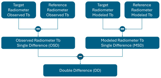
Figure 2.
XCAL double difference technique.
So, the mean DD is the desired radiometric calibration adjustment necessary to make the target PMR equal to the reference. In the limit of a large number of independent Tb observations, it is expected that the statistical probability distribution function (PDF) of these DDs is Gaussian, distributed about the “true” calibration offset (Tb bias). For a typical case, a single DD comparison has a high noise-equivalent delta-Tb (NEDT) of several Kelvin, which is the result of several independent random errors. Therefore, to meet the XCAL uncertainty goal (~0.1 K), typically >10,000 independent Tb measurements are required to reduce the uncertainty of the mean XCAL radiometric bias.
Moreover, referring to Figure 1, step 6, should any systematic dependance of the DD (XCAL bias) exist with scene, orbit, or radiometer instrument parameters, then the statistical central-limit assumption fails, and the double difference XCAL procedure cannot proceed. Therefore, it is necessary to verify the statistical independence of the DD comparisons. For this purpose, a large number of DD cases are subdivided into different subsets to verify that the resulting subset DD distributions have approximately the same means regardless of which DD values are used. For example, by dividing one year of DDs into monthly subsets, it is possible to verify statistical independence if there is no correlation with seasonal changes. Of course, cross-correlations with other variables must be performed, and any failure terminates the XCAL procedure. Thus, in this case, it is desirable to find the root cause of the “systematic radiometric calibration error” or, at least, to develop an empirical model that characterizes this error. Then, after applying this correction to the measured target Tbs, the mean of the resulting DD Gaussian PDF is the best estimate of the target calibration bias, relative to the reference radiometer.
2.2. XCAL Radiative Transfer Model
As discussed above, the DD method for Tb normalization between radiometers of different design utilizes the XCAL consensus microwave RTM to translate the measurement of one or the other to a common basis before comparison. When radiometers are of different designs, there may be significant differences in their radiances that are expected and do not necessarily constitute calibration errors. Thus, the use of the radiative transfer model allows the expected difference in the scene radiance to be determined.
Unfortunately, the physics of the measured observation may not exactly be represented in the RTM model used. Also, the RTM environmental inputs, oceanic and atmospheric parameters derived from numerical weather models, are imperfect estimates of the true values. Nevertheless, through the use of “double-differences” of the theoretical “modeled single difference” and the “observed single difference”, these RTM errors are common-mode and will tend to cancel. Of course, the degree of cancellation depends upon the similarity of the two radiometer receiver passbands. For radiometers operating within the atmospheric windows, that are removed from the 22 GHz water vapor and 50–70 GHz oxygen lines, the errors associated with common-mode cancellation effects are negligible.
Therefore, the most important characteristic of the XCAL RTM is that it accurately captures the dynamic change of the ocean scene radiance due to changes in radiometer frequency, earth incidence angle, and polarization, as well as changes in environmental parameters. Of the latter, sea surface temperature, wind speed, water vapor, and cloud liquid water are the most variable over space and time.
So, the XCAL consensus RTM uses the satellite radiometer viewing geometry to calculate the top-of-the-atmosphere (TOA) linearly polarized (V- and H-polarizations) brightness temperature for a homogeneous, clear-sky atmosphere/ocean scene. For microwaves, the effective limit of atmosphere emission/absorption is 20 km; therefore, atmospheric profiles from 27 pressure levels of the ERA5 environmental data are interpolated to centers of the 100 RTM layers of 200 m thickness (Note: XCAL uses a version of ERA5 which includes only 27 layers of ERA5 that correspond to 20 km). Because the lapse rates of the temperature, pressure, and water vapor have significant differences between the upper and lower RTM layers, interpolations are performed using a piece-wise linear distribution for temperature and piece-wise exponential distributions for pressure and water vapor.
The simplified RTM diagram, shown in Figure 3, accounts for the three TOA emission components, namely, polarized ocean surface emission, upwelling atmospheric emission, and downwelling atmospheric emission, which has specular reflection at the ocean surface. The TOA Tb is the scalar sum of these three components.

Figure 3.
Simplified microwave radiative transfer model.
2.3. RTM Physics
Originally, this XCAL RTM was used for conical scanning microwave imagers, which operated over the frequency range of 5 to 100 GHz. Because these remote sensors had similar earth-viewing geometries, the RTM was used to normalize these Tb observations to a common earth incidence angle (EIA). Also, because these radiometer frequencies were in the highly transparent to slightly opaque region of atmospheric transmissivity, the largest component of the TOA Tb was the polarized ocean surface emission with only a minor atmospheric attenuation correction. Also, the reflected downwelling atmospheric component was polarized by the ocean Fresnel coefficient, but the upwelling atmospheric com ponent was non-polarized. As a result, the major RTM emphasis was associated with the anisotropic rough ocean emissivity/reflectivity modeling [14] and with atmospheric continuum (non-resonant) absorption/emission associated with oxygen and nitrogen and resonant water vapor (WV) absorption/emission in the 22 GHz region [15,16,17].
Later, GPM XCAL activities were expanded to include millimeter wave (cross-track) sounding radiometers (>100 GHz), and the oxygen and water vapor resonant absorption/emission spectroscopy was improved [18]. This version, known as MonoRTM, uses the same physics as the Line by Line RTM (LBLRTM), with the exception that it is designed to process a limited number of monochromatic spectral output values, which decreases computational time. For a probability distribution for a layer-by-layer calculation of water vapor, oxygen, and nitrogen absorption coefficients, the MonoRTM uses a Voigt line shape on every atmospheric layer to describe the effects of pressure and Doppler line broadening [19]. Thus, for a given temperature profile and frequency, an optimal sampling of the atmospheric profile is possible using this method, and to achieve accuracy of better than 0.5%, a sampling interval of ¼ of line halfwidth is used [20]. For oxygen, there is an extremely strong absorption line at 60 GHz and a significantly weaker second harmonic at 120 GHz, and, for water vapor, there is a strong absorption line at the 183 GHz region.
2.4. TPX XCAL Results
The focus of this paper is to demonstrate the benefit of using an RTM for the XCAL of two satellite radiometers of different designs. Specifically, XCAL results are presented for a proposed GPM constellation satellite radiometer, Time-Resolved Observations of Precipitation structure and storm Intensity with a Constellation of Small satellites mission (TROPICS), with the GPM Microwave Imager, and this begins with a description of the two satellites and their respective radiometer sensors.
2.4.1. GPM Core Satellite
The GPM Core Observatory flies in a circular, 65° inclined, 408 km altitude, orbit that has approximately 16 revolutions per day. The GPM Microwave Imager is a multi-channel, conical-scanning, microwave radiometer with a measurement swath of 885 km, which is shown in Figure 4. For this paper, only the vertical polarized G-band (183 ± 3 GHz) channel is relevant, which has a double-sideband architecture with two 1 GHz passbands centered at 180.31 GHz and 186.31 GHz, respectively; and, note that neither passband contains the peak of the water vapor absorption line at 183.31 GHz. This channel has an earth incidence angle (EIA) equal to 49.2° and an antenna surface footprint of 6 km, with 226 contiguous azimuth beam positions (instantaneous field of view, IFOV) within the measurement swath.
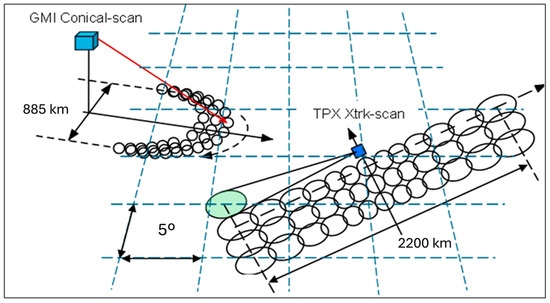
Figure 4.
GMI and TROPICS viewing geometry for Tb measurements.
2.4.2. TROPICS Satellite
TROPICS (hereafter identified as TPX) is cross-track scanning millimeter sounder that provides high-resolution imagery of the atmosphere (IFOV~16 km @ nadir and 34 km at edge of scan) using a constellation of five CubeSats flying in two 550 km altitude orbits. The first CubeSat launched was the “TROPICS Pathfinder” in a 97° sun-synchronous orbit, and this is the subject of this paper. This radiometer (Figure 4) measures the TOA radiance in 81 contiguous beam positions (± 60° range in incidence angle from nadir) that result in a 2200 km swath. There are two radiometers, W-band (120 GHz) and G-band (184 GHz), that share a common parabolic reflector, and the entire radiometer (receiver/antenna assembly) spins in the cross-track plane with a period of 3 s. Both radiometers have multiple bands, but only a single G-band radiometer channel, operating at 184.41 GHz with a bandwidth of 2.0 GHz, is used in this XCAL analysis.
2.4.3. Validation of the MonoRTM
For this study, it is important to estimate the uncertainty of the XCAL MonoRTM calculated brightness temperatures in the region of the 183 GHz water vapor absorption line. Since the water vapor absorption line is quite strong, when the total precipitable water (TPW) ≥10 mm, there are negligible (<0.1 K) ocean surface emissions and reflected downwelling atmospheric emissions at the top of the atmosphere. As a result, the RTM reduces to simply the non-polarized upwelling atmospheric component.
From the standpoint of millimeter wave atmospheric absorption spectroscopy, the MonoRTM has been experimentally validated [20], but there is a source of uncertainty related to differences between actual and ERA5-modeled atmospheric profiles of water vapor and temperature over oceans. Therefore, to validate the MonoRTM, we compared the observed brightness temperature from GMI with the modeled brightness temperature for a one-year period, and the results are shown in Figure 5. In the left panel, the brightness temperatures are averages over 5 mm bins of TPW retrieved from GMI by Remote Sensing Systems [21], and the right panel shows the difference between the observed (blue) and modeled (red) brightness temperatures in the left panel. These results demonstrate that the modeled brightness temperatures are in excellent agreement with the mean GMI observations, and the comparison with TPX is discussed next.

Figure 5.
Comparison of GMI-observed and -modeled TOA brightness temperatures (left panel) as a function of retrieved TPW from GMI simultaneous multi-channel observations. The right panel is the difference between the observed and modeled brightness temperatures, and the associated error bars are ±1 sigma values about the mean.
Since the radiometric calibration for the TPX is not validated, it is not possible to perform a similar comparison with MonoRTM. Moreover, relative to GMI, there are major differences in the atmospheric absorptions/emissions because the TPX passband is centered on the water vapor line, whereas GMI has two passbands centered ±3 GHz from the peak. Nevertheless, a qualitative comparison is made for the same GMI viewing geometry (equal path lengths), and results for one year of comparisons for TPX beam positions 11 and 71 are presented in Figure 6.
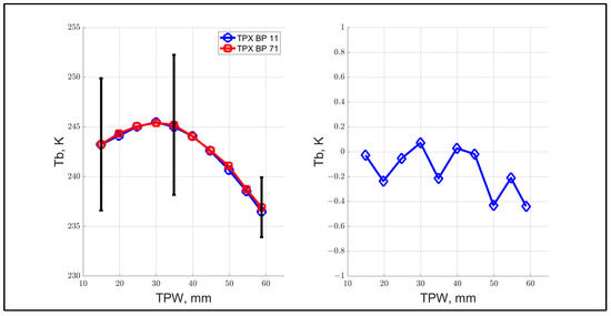
Figure 6.
Comparison of TPX-modeled TOA brightness temperature for beam positions 11 and 71, as a function of retrieved TPW from GMI simultaneous multi-channel observations. The right panel is the difference in modeled brightness temperatures, and the associated error bars are ±1 sigma values about the mean.
Consider the left panels of Figure 5 and Figure 6, which are similar in shape but have different brightness maximums. Given that the TPX passband is centered on the absorption line, the weighting function peak is higher in the atmosphere, and the observed maximum brightness difference of approximately 20 K lower than GMI is qualitatively consistent. Also, as expected for both, the brightness temperature dynamic ranges with TPW are approximately equal. Finally, the observation that the MonoRTM produces nearly identical results for two beam positions that occur at opposite sides of the swath (~2000 km separation) suggests the robustness of our XCAL approach. Therefore, considering these qualitative comparisons, it is concluded that the MonoRTM works equally well for TPX and GMI. Further, we believe that the DD results (observed SD minus modeled SD) presented below accurately represent the XCAL bias of TPX with respect to GMI.
2.5. TPX/GMI Match-Up Dataset
The creation of the match-up dataset involved the spatial/temporal collocation of TPX and GMI Tb measurements with associated environmental parameters (ERA5) and other ancillary data. As stated in Equation (1), the TPX brightness temperature measurements were a function of environmental parameters (primarily TPW), geometry, and radiometric calibration, all of which could change over time. So, several million GMI/TPX comparisons were required, over a one-year period, to verify that no systematic calibration errors existed in the TPX-measured brightness temperature.
A typical collocation of the TPX and GMI measurement swaths is shown for a single orbit in Figure 7, where the wider swath (blue) is for TPX, and the narrower swath (red) is GMI. The collocation area is the union of the two swaths, in the center of this orbit plot (between longitudes 150°E and 220°E), and this corresponds to a temporal match-up, which is typically <1 h. The other orbit crossing near zero longitude has a time difference of ~12 h, which is rejected. For this day, the descending GMI orbit segment (denoted by the downward pointing arrow) is collocated with the ascending orbit segment (denoted by the upward-pointing arrow) of TPX. On the other hand, all possible combinations of ascending and descending segments are possible within approximately a monthly cycle. Because the TPX orbit hosts the match-up grid, the naming convention is based upon the TPX orbit segment.
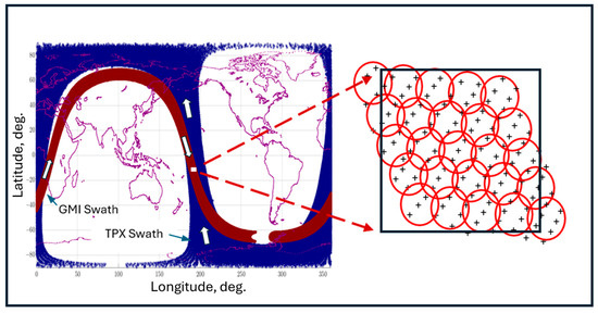
Figure 7.
Typical GMI (red) and TPX (blue) measurement swath collocations (left). Insert on right shows a single collocation grid “box” comprising five TPX scans by five TPX beam positions. Red circles are TPX IFOVs, and “+” symbols designate centers of GMI measurements.
The TPX and GMI measured Tbs were captured within a TPX moving cross-track grid (“box”) that is illustrated in the insert of Figure 7. The box spatial extent was five TPX beam positions (cross-track) by five TPX antenna scans (along-track), which is equivalent to the area of a fixed earth 0.5° latitude/longitude grid. Within each box, there were 25 TPX observations and approximately 80 GMI observations that were averaged to calculate a single observed Tb difference, OSD.
Also, using the ERA5 dataset closest to the average of the GMI/TPX times, the atmospheric and oceanic environmental parameters were interpolated to the corresponding box center. These data were the input to the MonoRTM that calculated the modeled Tb for both GMI and TPX, and, using Equation (3), the MSD was calculated.
Because the orbital periods of GMI and TPX were different, the geographic location of the match-ups changed on a daily basis, but, every day, the number of boxes was approximately equal. So, the OSD, MSD, DD, and ancillary parameters were combined in a data vector for each match-up box, and these were organized into a matrix database (>3 million boxes) for the year 2022.
3. Results
The TPX/GMI XCAL analysis was performed daily for this year, using two different approaches, namely, the observed single difference (OSD) and the double difference (DD). For each day, >30,000 collocations occurred, and these match-ups (boxes) were separated by ascending (daylight) and descending (nighttime) orbit segments of TPX orbits, as shown in Figure 7. Furthermore, the geographic location of these match-ups regions changed each day, with about a monthly repeat cycle, and, during this cycle, all combinations of ascending and descending orbit segments occurred, i.e., TPX ascending with GMI descending, TPX ascending with GMI ascending, and vice versa.
3.1. Single Difference
A typical example of the daily collocation swaths over oceans for TPX ascending orbit segments, is shown in Figure 8, where the spatial coverage is defined by the overlap of the closest orbits in time (typically <1 h), and the color scale is the box average observed Tbs for TPX (upper panel) and for GMI (lower panel). Next, the XCAL bias was calculated using OSD = Tb_tpx − Tb_gmi, and the results are displayed as the color scale in the upper portion of Figure 9. Also shown, in the lower panel of Figure 9, are the respective histograms of TPX and GMI Tbs, which differ significantly in their mean values.
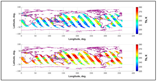
Figure 8.
Typical daily global ocean coverage for GMI/TPX match-ups for TPX ascending orbit segments. Color scale is measured Tb in Kelvin: for TPX (upper panel) and GMI (lower panel).
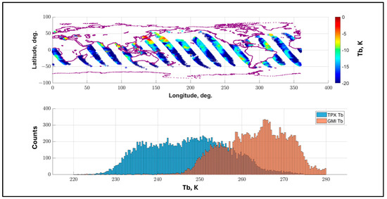
Figure 9.
Typical daily global ocean coverage for GMI/TPX match-ups for TPX ascending orbit segments (upper panel), with color scale equal the resulting OSD XCAL bias. Lower panel shows the corresponding histograms of observed brightness temperatures for TPX (blue) and GMI (red).
Recognizing that the GMI conical scanning geometry produces a constant incidence angle, the resulting Tb histogram dynamic range is caused by the global distribution of water vapor. On the other hand, TPX has a cross-track scanning geometry that results in a varying incidence angle and line-of-sight atmospheric path length that increases its Tb histogram dynamic range (i.e., the Tb variability is a function of both incidence angle and water vapor distribution). Also, the separation in the mean histogram values is the result of the water vapor absorption spectroscopy, as discussed in Section 2.4.3.
Referring to Figure 1, step 6, the OSD XCAL biases must be evaluated to ensure that no systematic dependances exist with scene, orbit, or radiometer instrument parameters. Obviously, the TPX-observed brightness varies with beam position (EIA), but, the radiometric calibration should be independent; and to verify this, the one-year match-up set was subdivided into 5° bins of EIA and GMI/TXP OSDs were calculated. For each beam position, there were >100,000 boxes, which were averaged by applying an iterative procedure to remove outliers and to estimate the mean and standard deviation for a best-fit Gaussian distribution within an observed Tb window of ±2.5 sigma about the mean.
The OSD results, plotted in Figure 10, show an approximately symmetrical distribution with TPX EIA about the nadir (beam position 41), which violates the assumption of independent random errors. Therefore, a reasonable solution was to characterize the systematic change in the measured Tb with EIA and to apply this correction before calculating the OSD. Because TPX matched the GMI EIA at beam positions 11 and 71, the zero-correction reference was their average value, and the resulting XCAL biases (versus EIA) are plotted in Figure 10 (red curve). So, after applying this TPX EIA normalization, the bias is “flat” (apparently independent of beam position).
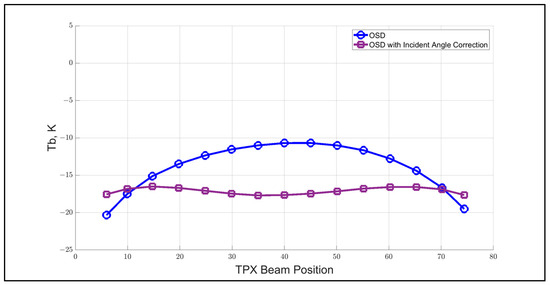
Figure 10.
OSD XCAL bias dependence on TPX beam position (blue curve) and corresponding XCAL bias with empirical EIA normalization applied (purple curve).
Next, we proceed with other analyses to assure that this EIA normalized OSD is free from other systematic effects. For this purpose, we divide the match-up dataset into TPX ascending (daylight) and descending (nighttime) orbit segments and compare corresponding OSDs. Consider first Figure 11, which is similar to Figure 10, with the exception that ascending and descending orbit segments are separated. Here, the beam-corrected OSD dependence on TPX beam position varied by only about ±1 K; and the separation between ascending and descending orbit segments exhibited a 0.3 K bias, which is significant but also not a major concern.
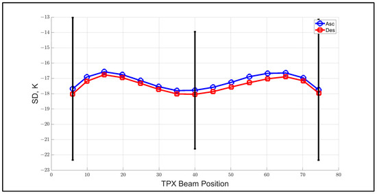
Figure 11.
Beam-corrected OSD XCAL bias dependence on TPX beam position (blue is ascending, red is descending), and error bars represent ±1 sigma standard deviation.
Next, OSD dependence on time (monthly), plotted in Figure 12, shows a random scattering of monthly values with zero mean slope, which also indicates no apparent dependency with time nor ascending or descending orbits.
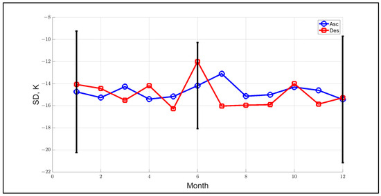
Figure 12.
OSD dependence on time (month) for 2022, where TXP ascending orbit segment is blue curve, and OSD descending orbit segment is red curve, and error bars represent ±1 sigma standard deviation.
However, considering Figure 13, the plot of OSD, with respect to TPW, indicates a systematic dependence showing a skewed quadratic trend for both ascending and descending orbit segments, which invalidates the assumption that only random calibration errors exist. Further, the large OSD dynamic range of about 8 K is not acceptable, and this demonstrates that the OSD alone is not sufficient for XCAL purposes.
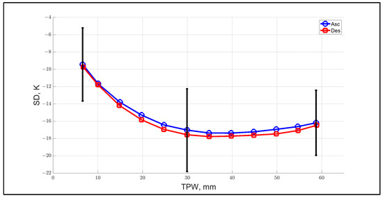
Figure 13.
OSD dependence on TPW for 2022. OSD ascending is blue curve, and OSD descending is red curve. Error bars represent ±1 sigma standard deviation.
Finally, the OSD dependence on latitude (shown in Figure 14) also indicates a similar systematic dependence, and this is expected given the strong correlation of TPW with latitude (above and below the equator). Also, the large dynamic range of about 8 K is unacceptable, and there is an apparent dependence on ascending and descending orbit segments, which is a minor issue. Thus, these results also support the conclusion that the OSD is insufficient for XCAL purposes.
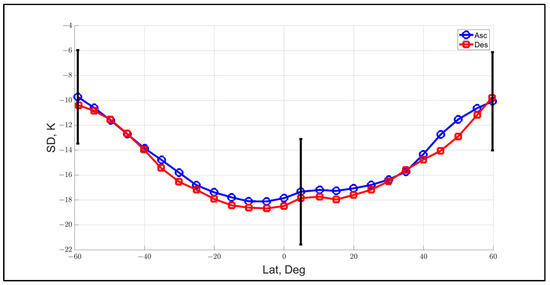
Figure 14.
OSD dependence on latitude for 2022. OSD ascending is blue curve, and OSD descending is red curve. Error bars represent ±1 sigma standard deviation.
3.2. Double Difference
This section presents the XCAL results for the same one-year dataset described above, but now using the DD approach to calculate the XCAL bias, which is the difference of the measured OSD and theoretical MSD. Also, note that the OSD used herein is the original, without the EIA normalization described above.
First, consider Figure 15, which shows the same global image of XCAL biases for TPX ascending orbit segments that was presented in Figure 9. Previously, the color scale represented the XCAL bias derived from the OSD, but now the biases are derived from the DD. Using the same color scale in this figure (±10 K), the biases are very uniform green color with a dynamic range of only ±2 K, which implies that the XCAL bias is constant and does not change significantly in either space or time.

Figure 15.
Typical daily global ocean coverage for GMI/TPX match-ups for TPX ascending orbit segments (upper panel), with color scale equal to the resulting DD XCAL bias. Lower panel shows corresponding histograms of the OSD (blue) and the MSD (red).
Next, consider the lower panel that compares the respective histograms of the box-average OSD and MSD for this day. The close similarity of these histograms indicates that the observed difference between PMRs closely matches their respective difference in theoretical values calculated by the MonoRTM. In fact, the MSD characterizes the difference in these two PMRs and defines how these two sensors should compare if they were “perfectly calibrated”. Thus, the RTM provides the robust normalization of these sensors before comparison, which accounts for differences in viewing geometry, as well as the atmospheric absorption effects within the different receiver passbands. Since these factors are present in both the observed and modeled TOA brightness temperatures, they are common-mode effects that cancel in the DD process.
Next, for the entire year, collocation boxes, subdivided by TPX beam position (EIA), were processed to produce binned averages of the DD, with respect to TPX beam position (Figure 16). As before (Figure 10), the OSD is the same “inverted parabolic curve” (blue), but now the MSD curve (green) is nearly identical, and the difference between these curves is the XCAL DD radiometric bias, which is plotted above in red. The DD bias curve is flat (peak to peak < 1 K), which indicates negligible systematic dependance on the TPX beam position.
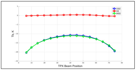
Figure 16.
Binned average OSD, MSD, and DD for one year of GMI/TPX match-ups, with respect to TPX beam position.
On the other hand, consider Figure 17, where DD biases results are shown separately for match-ups between TPX ascending and descending orbit segments. Here, there are two curves of near identical shapes that are separated by about 0.5 K. Since the number of boxes for each 5° EIA bin > 100,000, the uncertainty of the distribution mean is <0.1 K; therefore, a 0.5 K difference is significant. So, while this separation is small, this result is a concern because it indicates that there is a measurable difference associated with the ascending/descending orbit segments, which is not random.
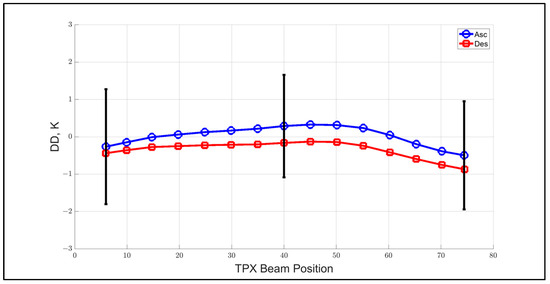
Figure 17.
Binned average DD with respect to TPX beam position, calculated for one year of GMI/TPX match-ups that are separated into TPX ascending (daytime) and descending (nighttime) orbit segments, and error bars represent ±1 sigma standard deviation.
Next, consider the monthly variability of the XCAL DD bias calculated separately for ascending (blue) and descending (red) for one year that is shown in Figure 18. Again, the two curves are separated, but the values are more randomly distributed, and, overall, the curves are flat, which does not indicate any systematic seasonal effects.

Figure 18.
Monthly binned average DD for one year of GMI/TPX match-ups that are separated into TPX ascending (blue) and descending (red) orbit segments, and error bars represent ±1 sigma standard deviation.
The last two comparisons are related to changes in the DD bias with TPW (Figure 19) and latitude (Figure 20), which are highly correlated, and these results are probably not independent. The atmospheric water vapor is highest at the equator, with a seasonal latitudinal swing (10° to 15°) of the inter-tropical convergence zone (ITCZ), based upon the hemisphere summer season. Also, as discussed above (Section 2.4.3), over oceans, low TPW (<15 mm) occurs primarily in the southern hemisphere at high latitudes, and, in this region, the MonoRTM calculations degrade because of uncertainties associated with ocean surface emission and antenna polarization mixing. Further, at high TPW > 50 mm, the modeled difference in GMI and TPX brightness temperatures diverge. Therefore, the TPW curves between 15 to 50 mm are the most reliable, and over this region, the DD curves exhibit a dynamic change of <0.5 K. However, concerning TPX ascending and descending orbit segments, the consistent separation of curves strongly suggests a systematic calibration error, which is not acceptable.
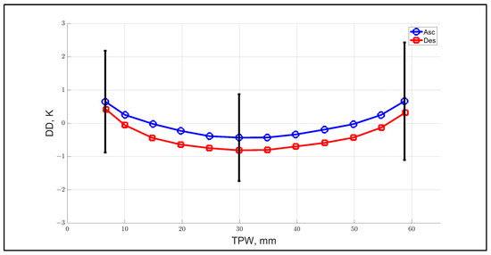
Figure 19.
Binned average DD with respect to TPW, calculated for one year of GMI/TPX match-ups that are separated into TPX ascending (daytime) and descending (nighttime) orbit segments, and error bars represent ±1 sigma standard deviation.
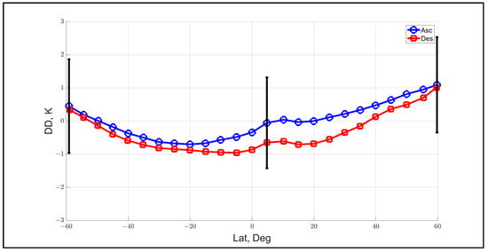
Figure 20.
Binned average DD with respect to latitude, calculated for one year of GMI/TPX match-ups that are separated into TPX ascending (daytime) and descending (nighttime) orbit segments, and error bars represent ±1 sigma standard deviation.
Considering Figure 20, the change in DD with latitude appears to be significant, which suggests a systematic calibration error. Obviously, the radiometer calibration is not a function of latitude, but there are physical factors, such as instrument physical temperature, which changes with latitude, that could be the root cause. Also, because of the extent of the Pacific Ocean, latitudes between −60 and −40 contribute a larger % of the match-up boxes, and these are associated with low TPW and minimum instrument physical temperature, which may bias the results. Also, there is a notable feature between 10° to 15° latitude (probably associated with the ITCZ), which may be contaminated by rain. Also, the separation of the ascending and descending curves (about 0.5 K) supports the existence of a systematic calibration error that could adversely affect the XCAL bias.
4. Discussion
4.1. Comparison of Single Difference and Double Difference XCAL
As discussed above, for the OSD technique, an ad hoc EIA normalization was applied to the observed brightness temperatures, and, afterwards, based upon one year of observations, the resulting OSD was nearly constant for all beam positions. However, when examining the OSD as a function of the coincident TPW value, a significant systematic dependance was discovered (Figure 13). Because this condition violated the assumption of having only random calibration errors, the calculation of the XCAL bias using the OSD approach was rejected.
On the other hand, the DD technique performed much better, and the intercomparisons of these two XCAL techniques are presented in Figure 21 and Figure 22. These results support using the RTM to account for differences in the spectrum of the emissions captured by the respective radiometers. For GMI/TPX comparisons, even though both radiometers measure the same water vapor absorption line, their passbands occur over different portions of this resonance and thereby affect the respective measured atmospheric emissions. Clearly, having the RTM to calculate the expected Tb, for both sensors, makes their contribution a common-mode factor that cancels in the difference process. Even if there are errors in the absorption physics or the input environmental parameters, both modeled Tbs are affected, and, in the MSD process, these errors are significantly reduced if not totally cancelled.
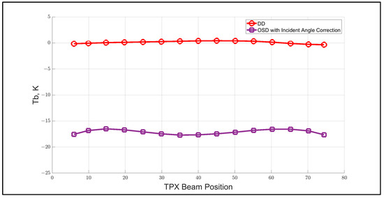
Figure 21.
Comparison of the modified OSD (lower curve) and the DD XCAL techniques (upper curve) in the XCAL bias determination.

Figure 22.
Comparison of the modified OSD (lower curve) and the DD XCAL techniques (upper curve) in the XCAL bias determination as a function of retrieved TPW, and error bars represent ±1 sigma standard deviation.
4.2. Anomalous Regions-Radiometer Tb Anomaly Determination
During the conduct of this investigation, it was discovered that, on occasion, the calibration of the TPX radiometer exhibited anomalous “step-function” changes, which lasted for periods of approximately one orbit. For example, consider the upper panel of Figure 23, an image of TPX DD bias for ascending orbit segments on 19 January 2022. In the southern hemisphere Pacific Ocean, there are two regions (orbit 6 and 9) with anomalously large DD biases (shown in red).

Figure 23.
Global ocean coverage (19 January 2022) for GMI/TPX match-ups for TPX ascending orbit segments (upper panel), where color bar represents the DD values. Lower panel shows histograms for OSD (blue) and MSD (red).
Now, consider Figure 24, an expanded image of Figure 23, where all orbits are removed except three that show a “good orbit 8” with low DD bias (green color) at longitude 220E, which is surrounded by two “bad orbits, 6 (right) and 9” (left) with high DD biases (red color). Note that for orbit 9, the anomalous region is located south of the equator; so, this orbit was separated into two sections, above and below latitude −2.5°. Next, for these orbit segments, the average XCAL bias was calculated in 5° bins of TPX cross-track beam positions, and the results are presented in Figure 25. In this figure, there are two sets of curves that are separated and flat, with respect to beam position, which indicates that the anomaly is constant over a TPX scan. Because the TPX radiometer is calibrated once per scan, this suggests that the anomaly may be related to the noise-injection procedure used for calibration. Note that the DD for good orbit 8 and the higher latitude portion of bad orbit 9 are in excellent agreement with the DD biases from January 20. Finally note that there is a clear separation of the anomalous results (orbits 6 and 9) compared to the good orbits, which shows that the DD approach is superior in detecting anomalous XCAL results.
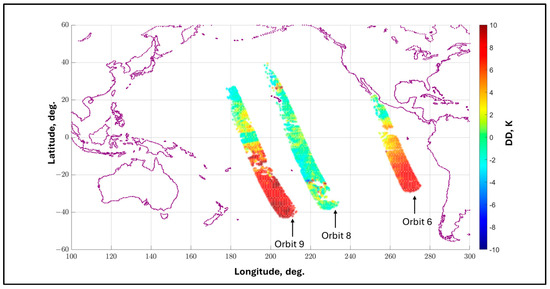
Figure 24.
Expanded image of XCAL DD biases for 19 January 2022, showing regions of anomalous TPX Tbs, where, from right to left, are orbits 6, 8, 9.

Figure 25.
TPX XCAL DD biases averaged in 5° cross-track boxes for orbits 6, 8, 9 on 19 January 2022. Lower curves are for “good orbit segments” and upper curves are for anomalous orbit segments.
To understand the cause of the anomalous DD condition, it is necessary to establish whether individual single difference components or their combination is the cause; therefore, the OSD and MSD are analyzed separately for orbits without and with anomalies on January 19. For the TPX ascending segment orbit 8 (without anomalous DDs), the TPX Tb histograms are given in Figure 26 (upper left panel), and the GMI Tb histograms are given in Figure 26 (upper right panel). For both radiometers, the observed and modeled histograms match well, which results in small OSD, MSD, and DD values for this orbit. The resulting cross-correlation between upper and lower Tb histograms were 0.96 with a lag of −2 deg K for TPX and 0.97 with zero lag for GMI.
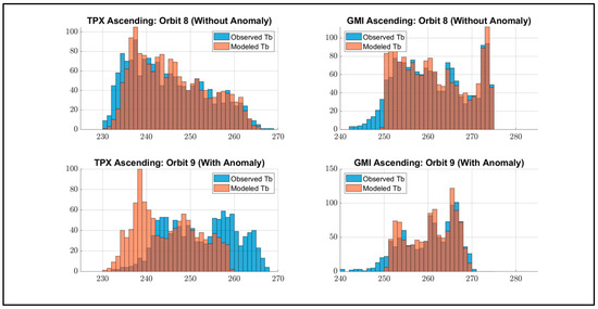
Figure 26.
Observed and modeled Tb histograms for 19 January 2022, for TPX ascending orbit segments. Upper panel is orbit 8 (without anomaly) and lower panel is orbit 9 (with anomaly), and left side is TPX (OSD and MSD) and right side is GMI (OSD and MSD).
Now, consider the lower half of Figure 26, which shows TPX ascending orbit 9 (orbit with anomalous DDs). For GMI (lower right panel): the observed and modeled histograms match well. On the other hand, for TPX (lower left panel), the modeled Tb histogram (blue) is shifted right (8 K) relative to the upper left panel, which results in a larger OSD. For the TPX-modeled Tb histograms (red), both lower left and upper left match well, which demonstrates that the anomalous DD is the result of bogus TPX Tb measurements. Based upon the cross-correlation of the histograms, TPX had a correlation coefficient of 0.93, and the peak correlation indicated a shift of +8 deg K, and GMI had a correlation coefficient of 0.97 and the peak correlation indicated no shift in K.
Next, consider the corresponding descending orbit segments for 19 January, shown in the upper panel of Figure 27, where large regions of anomalous low values of DD (blue) occurred for orbits 4, 5, and 9. It is noted that anomalous cases for ascending and descending orbit segments have different DD bias polarities, namely, positive for ascending and negative for descending for 19 January. This association with higher polarity with ascending and lower polarity with descending is not a consistent phenomenon throughout the entire year, and the polarity reverses on other days.
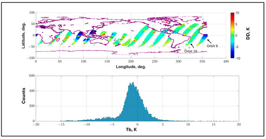
Figure 27.
Global ocean coverage (19 January 2022) for GMI/TPX match-ups for TPX descending orbit segments (upper panel), where color bar represents the DD values, and the lower panel shows histograms for DD.
Following the approach discussed above, GMI and TPX Tb histograms for TPX descending orbit segments were also examined, and the results are shown in Figure 28 using the same format as Figure 26, which shows orbits without anomalies in the upper panels and orbits with anomalies in the lower. For orbit 8 (without anomaly), TPX is the upper left panel and GMI is the upper right. For both OSD and MSD, the histograms match well and are highly correlated, which agrees with the previous results for TPX ascending.
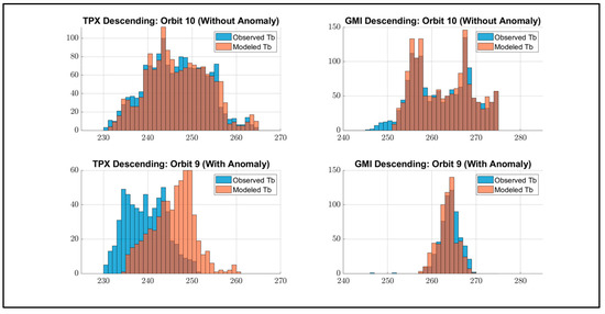
Figure 28.
Observed and modeled Tb histograms for 19 January 2022 for TPX descending orbit segments. Upper panel is orbit 8 (without anomaly) and lower panel is orbit 9 (with anomaly), and left side is TPX (OSD and MSD) and right side is GMI (OSD and MSD).
On the other hand, results are also presented in Figure 28 for TPX orbit9 (anomaly) in the lower left panel. Here, the results are the same as before (Figure 26), except that the TPX-observed Tb histogram (blue) is now shifted left (−6 K) relative to the corresponding upper panel. As before, the GMI histograms match well. The cross-correlation results of the observed and modeled Tb histograms were 0.94 with a negative lag of −6 deg K for TPX and 0.96 with positive lag of +2 K for GMI.
Finally, the process continued to identify the probability for the occurrence of these TPX anomalies. Since this anomaly was caused solely by the TPX-observed Tbs, and since the TPX-modeled Tbs were generally validated during the DD process, there was no need to continue GMI in this process. As a result, the investigation examined the Target Single Difference (TSD), defined as the TPX-observed Tb minus the TPX-modeled Tb. This expanded the match-up process to include the entire TPX swath, which more than doubled the number of boxes. While the root cause of this systematic error is still under study, the ability of the TSD technique to identify anomalous Tbs is a valuable feature. Also, for this analysis, TPX observations over land were used, since it was determined that the contribution of surface-level emission to the TOA brightness temperature was negligible for TPW > 10 mm. Consider Figure 29, which shows the TSD for TPX ascending orbit 9 (seen in Figure 25 as a DD). It is important to note that the anomaly is present throughout the entire orbit and not just a part of the orbit
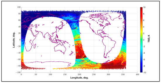
Figure 29.
TPX orbit 9 (with anomaly) 19 January 2022, where color scale represents the TSD value.
An evaluation procedure was developed to detect the anomaly occurrence, which was based on the comparison of the time series of swath-average TSD with the corresponding instrument temperature, and an example is presented for January 19 in the upper panel of Figure 30. The instrument temperature varies sinusoidally over the orbit period because the ascending orbit segment is daytime, and descending is nighttime. If temperature were a factor in the TPX anomaly, then it should be readily apparent from these time-series plots. Unfortunately, this is not the case for the TPX anomaly that occurs between 350 and 500 min. Moreover, the TPX data record also has the associated noise calibration NEDT measurements (green = hot) and (magenta = cold), which are also plotted. Since there is an obvious increase in the NEDT during the anomaly period, there is an ongoing investigation to establish the root cause of the Tb anomaly.
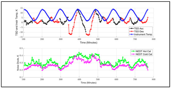
Figure 30.
Time series of instrument physical temperature, TPX swath average TSD, and calibration noise diode NEDT for 19 January 2022.
5. Conclusions
Based upon the results presented for two different approaches, namely, with and without the use of a RTM, the following inter-satellite radiometric calibration conclusions are reached:
5.1. Observed Single Difference Method
The observed single difference (OSD) approach for XCAL can accurately determine the relative radiometric bias between two radiometers, when (1) they simultaneously view a homogeneous earth scene and (2) when they have identical passbands over which the spectral radiance is averaged. The first (simultaneous) condition assures that the scene spectral radiance does not change due to a propagating weather system, and the second (homogeneous) condition is to assure that there are no differences associated with the spatial collocation of respective IFOVs. Finally, the third condition is to ensure that the integral of the spectral radiance over the passbands are equal. Concerning the latter, when the spectral radiance is flat with frequency, then the condition can be relaxed because the brightness temperature is based upon the average over the passband.
On the other hand, when radiometers are not identical in design (frequency, passband, polarization, and geometry), then significant biases may result. The reason for this is that spectral radiance changes with both geometry and environmental parameters, and the change in associated brightness temperatures for the two radiometers will not necessarily cancel in the OSD.
In this paper, the GMI/TPX XCAL example is of the latter case. Even though both radiometers have a total of 2 GHz passband, the location in frequency is very different. While both receiver passbands included the same water vapor absorption line, the corresponding integrals over their passbands was considerably different, as noted in the observed TOA Tb histograms shown in Figure 9. As a result, the OSDs calculated in match-up boxes were variable with both the known geometry (EIA) and with the unknown scene environmental parameters. However, when one year of TXP/GMI match-ups were subdivided by beam position and averaged over all scenes, the result was a stable set of XCAL biases that systematically varied by beam position (Figure 10).
To remove this systematic dependance, an empirical EIA normalization was developed that adjusted the observed Tb with respect to the EIA of GMI. Applying this to the observed TPX Tbs resulted in an OSD bias that was nearly constant and independent of beam position, as shown in Figure 10. However, in subsequent comparisons, the match-up data were subdivided by other parameters (e.g., ascending and descending orbit segments, month of year, scene TPW, and latitude). When using these different subsets, the resulting OSD bias was not a constant (see Figure 11, Figure 13 and Figure 14). These results show that the simple 1D normalization by EIA was not sufficient to remove the systematic dependences with other parameters that are associated with the scene Tb.
5.2. Double Difference Method
For this technique, the XCAL between TPX and GMI was very successful despite the significant differences in the PMR designs and measurement geometry, and the empirical results shown in Figure 16 demonstrated the advantage of the DD process. As shown in Figure 1, the MonoRTM was used to model the theoretical responses of the two sensors, and then the MSD was calculated. So, the subtraction of the MSD normalized the TPX sensor to be an equivalent of GMI (i.e., the MSD was the expected change in the observed Tb single difference (OSD) for a given scene). When using one year of matchups, the DD was compared by beam position (EIA) in Figure 16, and the resulting curve was flat without apparent dependence on beam position. Despite this, the DD was not without its flaws, because, in subsequent comparisons, where the match-up data were subdivided by other parameters, the resulting DD bias was not a constant (see Figure 17, Figure 18, Figure 19 and Figure 20). Nevertheless, these DD results were far superior compared to those using the OSD, as shown in Figure 21.
Given the large number of match-up boxes (>3 million), we conclude that the XCAL bias uncertainty is <0.1 K, which is the XCAL goal. This is based on modeling the DD as a Gaussian PDF about the true radiometric bias. Given this, the worst-case uncertainty of the estimated mean was determined using the GMI-observed minus -modeled Tb histogram for one year. For this histogram, the mean = −0.14 K, the standard deviation (std) = 2.11 K, and the number of boxes was >3 million. Using the (standard deviation)/(square root of the number of boxes), the uncertainty was ±0.002 K. This is the total uncertainty of the GMI-observed and -modeled Tb, which we assume is equal to the MonoRTM uncertainty (worst case). Next, this procedure was repeated using the TPX DD bias histogram, mean = −0.364, std = 1.48, and the number of boxes/5° EIA bins was 185,000, and the calculated uncertainty was ±0.0048 K, which we assumed was for the MonoRTM (worst case). Because the variance of the DD is the sum of the variance of the OSD and the MSD, the DD standard deviation is ±0.0049 K, which we round up to 0.01 K.
Concerning the anomalous TPX-measured Tb, we suspect that the issue is an unknown systematic error associated with either the transfer function (radiometer output counts to Tant) or the radiometric calibration (gain and offset). For example, in Figure 30, the time series of DD clearly captures the effect of the Tb anomaly, which is a step-function change in the radiometer calibration for a period of 1 to 1.5 orbits. Note that there is an change in the cold- and hot-point NEDT that is also associated with the anomalous period. Further, for non-anomalous orbits, there appears to be a smaller change in the DD signal associated with the ascending/descending orbit segments. Unfortunately, this is an ongoing investigation, so this error cannot be removed at this time.
From a statistical standpoint, over one year, the TPX performed well for about 97% of the time; however, from the GPM scientific utility, the anomaly was not randomly distributed over time. Because occasional orbits produce bogus results, they cast doubts on the utility of all measurements. So, because we cannot assure that the worst case has been demonstrated, until such time that the root cause for the anomaly is identified, the incorporation of TPX pathfinder into the GPM constellation is not recommended. However, it is reasonable to expect that an anomaly quality flag may be developed using the TSD, and then the objections to using TPX will be significantly diminished.
Author Contributions
All authors contributed to this paper. P.N.D.L.L. performed the analysis of the radiative transfer model, simulations, analysis of the results, and the writing of the manuscript. F.B.K. assisted with the analysis of the radiative transfer model and editorial adjustments. W.L.J. was the advisor and provided technical expertise, guidance, and help with the writing of the manuscript. All authors have read and agreed to the published version of the manuscript.
Funding
This research was funded under grant number 80NSSC23K0061 from NASA Goddard Space Flight Center titled “Inter-Satellite Radiometric Calibration for TROPICS”.
Data Availability Statement
The data used was provided via the XCAL working group from NASA Goddard Space Flight Center.
Acknowledgments
We thank NASA Goddard Space Flight Center for providing data, funding, and support.
Conflicts of Interest
The authors declare no conflicts of interest.
References
- Biswas, S.K.; Farrar, S.; Gopalan, K.; Santos-Garcia, A.; Jones, W.L.; Bilanow, S. Intercalibration of Microwave Radiometer Brightness Temperatures for the Global Precipitation Measurement Mission. IEEE Trans. Geosci. Remote Sens. 2013, 51, 1465–1477. [Google Scholar] [CrossRef]
- Hollinger, J.P. Special Sensor Microwave/Imager Calibration and Validation; Final Report; Defense Technical Information Center: Fort Belvoir, VA, USA, 1989; Volume 1, 196p. [Google Scholar]
- Hollinger, J.P.; Peirce, J.L.; Poe, G.A. SSM/I Instrument Evaluation. IEEE Trans. Geosci. Remote Sens. 1990, 28, 781–790. [Google Scholar] [CrossRef]
- Hollinger, J.P. (Ed.) DMSP Special Sensor Microwave Imager Calibration/Validation; Final Report; Naval Research Laboratory: Washington, DC, USA, 1991; Volume 2. [Google Scholar]
- Colton, M.C.; Poe, G.A. Intersensor Calibration of DMSP SSM/I’s: F-8 to F-14, 1987–1997. IEEE Trans. Geosci. Remote Sens. 1999, 37, 418–439. [Google Scholar] [CrossRef]
- Hong, L.; Jones, W.L.; Wilheit, T.T.; Kasparis, T. Two Approaches for Inter-Satellite Radiometer Calibrations Between TMI and WindSat. J. Meteorol. Soc. Jpn. 2009, 87A, 223–235. [Google Scholar] [CrossRef]
- Chen, R.; Jones, W.L. Creating a Consistent Multi-Decadal Oceanic TRMM-GPM Brightness Temperature Record with Estimated Calibration Uncertainty. Climate 2020, 8, 31. [Google Scholar] [CrossRef]
- Hou, A.Y.; Kakar, R.K.; Neeck, S.; Azarbarzin, A.A.; Kummerow, C.D.; Kojima, M.; Oki, R.; Nakamura, K.; Iguchi, T. The Global Precipitation Measurement Mission. Bull. Am. Meteorol. Soc. 2014, 95, 701–702. [Google Scholar] [CrossRef]
- Huffman, G.J.; Adler, R.F.; Morrissey, M.M.; Bolvin, D.T.; Curtis, S.; Joyce, R.; McGavock, B.; Susskind, J. Global precipitation at one-degree daily resolution from multisatellite observations. J. Hydrometeor. 2001, 2, 36–50. [Google Scholar] [CrossRef]
- Huffman, G.J.; Bolvin, D.T.; Nelkin, E.J.; Wolff, D.B.; Adler, R.F.; Gu, G.; Hong, Y.; Bowman, K.P.; Stocker, E.F. The TRMM Multisatellite Precipitation Analysis (TMPA): Quasi-global, multiyear, combined-sensor precipitation estimates at fine scales. J. Hydrometeor. 2007, 8, 38–55. [Google Scholar] [CrossRef]
- Grecu, M.; Olson, W.S.; Munchak, S.J.; Ringerud, S.; Liao, L.; Haddad, Z.; Kelley, B.L.; McLaughlin, S.F. The GPM Combined Algorithm. J. Atmos. Ocean. Technol. 2016, 33, 2225–2245. [Google Scholar] [CrossRef]
- Berg, W.; Bilanow, S.; Chen, R.; Datta, S.; Draper, D.; Ebrahimi, H.; Farrar, S.; Jones, W.L.; Kroodsma, R.; McKague, D.; et al. Intercalibration of the GPM Microwave Radiometer Constellation. J. Atmos. Ocean. Technol. 2016, 33, 2639–2654. [Google Scholar] [CrossRef]
- Ruf, C.S. Detection of Calibration Drifts in Spaceborne Microwave Radiometers Using a Vicarious Cold Reference. IEEE Trans. Geosci. Remote Sens. 2000, 38, 44–52. [Google Scholar] [CrossRef]
- Meissner, T.; Wentz, F.J. The Emissivity of the Ocean Surface Between 6 and 90 GHz over a Large Range of Wind Speeds and Earth Incidence Angles. IEEE Trans. Geosci. Remote Sens. 2012, 50, 3004–3026. [Google Scholar] [CrossRef]
- Rosenkranz, P. Absorption of Microwaves by Atmospheric Gases; John Wiley & Sons: New York, NY, USA, 1993. [Google Scholar]
- Liebe, H.J.; Rosenkranz, P.W.; Hufford, G.A. Atmospheric 60-GHz Oxygen Spectrum: New Laboratory Measurements and Line Parameters. J. Quant. Spectrosc. Radiat. Transf. 1992, 48, 629–643. [Google Scholar] [CrossRef]
- Rosenkranz, P.W. Water Vapor Microwave Continuum Absorption: A Comparison of Measurements and Models. Radio Sci. 1998, 33, 919–928. [Google Scholar] [CrossRef]
- Moncet, J.L.; Clough, S.A. Accelerated Monochromatic Radiative Transfer for Scattering Atmospheres: Application of a New Model to Spectral Radiance Observations. J. Geophys. Res. Atmos. 1997, 102, 21853–21866. [Google Scholar] [CrossRef]
- Turner, D.D.; Tobin, D.C.; Clough, S.A.; Brown, P.D.; Ellingson, R.G.; Mlawer, E.J.; Knuteson, R.O.; Revercomb, H.E.; Shippert, T.R.; Smith, W.L.; et al. The QME AERI LBLRTM: A Closure Experiment for Downwelling High Spectral Resolution Infrared Radiance. J. Atmos. Sci. Nov. 2004, 61, 2657–2675. [Google Scholar] [CrossRef]
- Draper, D.W.; Newell, D.A.; McKague, D.S.; Piepmeier, J.R. Assessing Calibration Stability Using the Global Precipitation Measurement (GPM) Microwave Imager (GMI) Noise Diodes. IEEE J. Sel. Top. Appl. Earth Obs. Remote Sens. 2015, 8, 4239–4247. [Google Scholar] [CrossRef]
- Wentz, F.J.; Meissner, T.; Scott, J.; Hilburn, K.A. 2015, Remote Sensing Systems GPM GMI [Yearly] Environmental Suite on 0.25 Deg grid, Version 8.2. Remote Sensing Systems, Santa Rosa, CA. Available online: www.remss.com/missions/gmi (accessed on 16 February 2024).
Disclaimer/Publisher’s Note: The statements, opinions and data contained in all publications are solely those of the individual author(s) and contributor(s) and not of MDPI and/or the editor(s). MDPI and/or the editor(s) disclaim responsibility for any injury to people or property resulting from any ideas, methods, instructions or products referred to in the content. |
© 2025 by the authors. Licensee MDPI, Basel, Switzerland. This article is an open access article distributed under the terms and conditions of the Creative Commons Attribution (CC BY) license (https://creativecommons.org/licenses/by/4.0/).