Abstract
Moisture transports play a key role in maintaining the hydrometeorological cycle and forming its climate variability over the Tibetan Plateau (TP), also known as the “Asian water tower”. This study focuses on understanding the interannual variability mode characteristics of moisture transport in the TP in boreal summer, using satellite-based analysis and reanalysis data from 1983 to 2022 with a combined empirical orthogonal function (EOF) analysis. We identified the first two primary interannual modes of TP summer water vapor fluxes, which are primarily characterized by zonal and meridional dipole patterns, respectively. The zonal pattern of the TP water vapor flux dominates the TP and East Asian summer rainfall variability, while the meridional pattern of the TP water vapor flux tends to be a result of the South Asian summer rainfall and its circulation anomalies. The tropical Indo-Pacific sea surface temperature (SST) variations, such as El Niño and Indian Ocean SST modes, have significantly delayed relationships with the interannual variability modes of the summer water vapor fluxes over the TP, indicating a significant modulation effect of the low-latitude oceanic variability on the interannual variations in TP summer moisture transport. These results deepen our understanding of the relationship between TP moisture transport and summer monsoonal rainfall variability, as well as the influence of the tropical oceans.
1. Introduction
As the “Water Tower of Asia” [1,2], the Tibetan Plateau (TP) plays a crucial role in the global water cycle and serves as the primary source of most major Asian rivers. It provides vital freshwater resources for over 1.4 billion people in downstream regions while also significantly influencing the ecosystems of our country [3]. With the TP as the “roof of the world”, its dynamic and thermal forcing significantly affects the occurrence and development of climate and weather events in China and East Asia. In particular, the “air pump” suction of the uplifting plateau terrain [4] can drive the warm and humid air transporting from the tropical oceans to TP, resulting in the high water vapor content over TP and its surrounding in boreal summer, forming an atmospheric “wet pool”, known as the “atmospheric water tower” [5]. The TP precipitation is mainly distributed in the southeastern part [6], gradually declining towards the northern and western TP [7]. The thermal forcing on the TP can be attributed to large-scale atmospheric teleconnections, such as the Asia–Pacific Oscillation in summer [8], which brings cyclonic circulation anomalies with southwesterly and southerly anomaly winds from Africa to East Asia in the lower troposphere [9]. The abnormal changes in the atmospheric heat status in the TP are closely related to East Asian atmospheric circulation. Zhao and Chen [10] found that there were significant positive correlations between the TP heat source and precipitation over the Yangtze River Basin.
Spatial and temporal variations in moisture over the TP in summer drive the local water cycle processes [11]. Moreover, adequate moisture supply is essential for precipitation generation and influences atmospheric moisture content. Moisture content and transport play crucial roles in precipitation formation. The water vapor budget over the TP is affected by the South Asian monsoon, East Asian monsoon, mid-latitude westerly winds, and other circulation systems. Therefore, examining the characteristics and influencing factors of TP moisture transport is of great significance for understanding changes in the hydrometeorological cycle and the ecological environment of surrounding regions. There are two main sources of moisture transport in the TP during the summer, the Indian summer monsoon [1,12] and the mid-latitude westerlies [13], which are clearly evident in the climatological distributions of vertically integrated water vapor fluxes and divergence over the TP (Figure 1). The strongest moisture transport originates from the Arabian Sea and Bay of Bengal through the South Asian monsoon system. In a study on the interannual oscillatory variability of moisture over the TP, Liu [11] found that in terms of temporal variability, the summer moisture balance exhibits 7–12-year cycle. Similarly, Meng [14] demonstrated that the summer moisture balance over the TP in the past two centuries has primarily been characterized by quasi-4–6-year interdecadal variability.
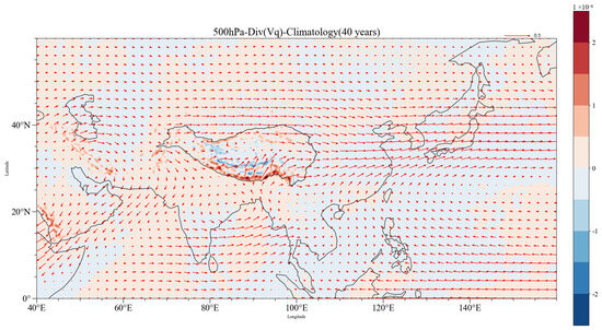
Figure 1.
Climatology distribution of water vapor fluxes (arrow vectors) at 500 hPa over TP (unit: kg/) in summer of 1983–2022.
So how is the spatial and temporal variability of summer precipitation characterized over the TP? What is the relationship between precipitation changes and moisture flux? Several studies indicate that summer precipitation over the TP exhibits significant interannual variability, with its spatial distribution displaying an east–west dipole pattern along the monsoon boundary [14,15]. The southeastern plateau typically experiences the highest precipitation amounts during summer [6,16]. Meanwhile, it is found that the spatial modes of precipitation in the north and south of the TP in summer have obvious north–south dipole variations, which can also be called “see-saw” modes [15,16,17]. Many studies have investigated the relationship between the moisture transport over the TP and oceanic processes [18,19,20,21,22,23,24,25,26,27]. Through the cooperative interaction of westerly winds and monsoons, the tropical oceanic water vapor source forms an interaction with the river, lake, and glacier systems on the TP, thus contributing to a specific global atmospheric water cycle process [28]. In addition, El Niño and Southern Oscillation (ENSO) in the Pacific can lead to anomalies in the Walker circulation over the Indian Ocean warm Pool, further affecting the Indian Ocean Dipole (IOD) [27]. Numerous studies have explored the influence of air–sea interactions in the Indian and Pacific Oceans on precipitation changes over the TP and its surrounding areas [18,19,20,21,22,23,24,25,26,27].
For the role of the Indian Ocean, moisture from the equatorial Pacific is transported to the southern part of the TP under the influence of the Indian summer winds, which affects the interannual variability of summer precipitation on the TP. Specifically, the Indian summer winds further regulate moisture transport processes in the Yarlung Tsangpo River Basin by influencing the circulation north of the monsoon zone. For the role of the Indo-Pacific warm pool, anormal moisture can be transported from the warm ocean during the boreal summer to the southeastern TP and the Yunnan–Guizhou Plateau, resulting in increased precipitation in the southeastern TP. When the eastern part of the Pacific warm pool was warmer, the western North Pacific subtropical high (WNPSH) was stronger and shifted further west, transporting more moisture to the southeast of the TP via the South China Sea. When the western Indian Ocean was warmer, more moisture entered the TP through the Bay of Bengal [28,29]. On the interannual timescale, the Indian Ocean basin mode (IOBM) and the IOD of SST variability exhibited distinct seasonal phase-locking features that affected the water vapor convergence and precipitation in the southeastern TP through changing the latent heat flux [30]. On an interdecadal scale, for the Pacific Ocean, the characteristics of the Pacific Decadal Oscillation (PDO) are consistent with the interdecadal variability of summer precipitation and moisture fluxes at the TP. The SST anomalies in the Pacific, Indian Ocean, as well as the North Atlantic Oscillation (NAO), influenced monsoonal circulation, thereby affecting precipitation variations over the TP and surrounding regions [31,32,33,34,35,36,37]. A study by [11] revealed a significant correlation between ENSO/NAO indices and interdecadal moisture variability in the central and southeastern TP.
However, few studies have examined the relationship between primary interannual variability modes of summer moisture transports in the TP and the thermal states of the low-latitude oceans on an interannual timescale. Therefore, this study investigates the primary interannual modes of TP summer water vapor fluxes and their relationships with surrounding moisture variables and external oceanic phenomena. We found the top two most important dominant modes of moisture flux by performing a Combined-EOF analysis of the components of the summer moisture flux over the TP, which represent the vast majority of the percentage of moisture transport over the TP. The results are made clearer by separating out these two modes and each looking for important oceanic regions. The remainder of this paper is structured as follows: Section 2 briefly introduces the data and analysis methods. Section 3 provides the characteristics of primary moisture transport modes, investigates the associated variable features, and presents the relationship between TP moisture transport modes and tropical SST indices. Summary and discussions are given in Section 4 and Section 5.
2. Materials and Methods
2.1. Materials of Observation Datasets
The monthly vertical integral of eastward water vapor flux, vertical integral of northward water vapor flux, vertically integrated moisture divergence, geopotential height, zonal/meridional wind, surface sensible heat flux, surface latent heat flux, and sea surface temperature (SST) are derived from the European Centre for Medium-Range Weather Forecasts Reanalysis v5 (ERA5), with a horizontal precision of 0.25° × 0.25° grid. Here, we use the monthly mean data for the boreal summer (June to August, JJA) from 1983 to 2022.
Due to the complex topography, unique altitude of the plateau, and the lack of meteorological observation data, Outgoing Longwave Radiation (OLR, unit: W/) data are widely used to study the correlation between the strength and variability of TP convection. The low center of the OLR in summer is located southeast of the TP, which is related to strong convection and precipitation in summer [38]. In this study, we use the monthly mean OLR data observed by National Oceanic and Atmospheric Administration (NOAA) series satellites from 1983 to 2022, with a horizontal resolution of 2.5° × 2.5°, to analyze the OLR fields over the TP and surroundings. We also use precipitation data from the Global Precipitation Climatology Project (GPCP) from 1983 to 2022, which provides a consistent analysis of global precipitation from an integration of various satellite data sets over land and ocean and a gauge analysis over land. on a 2.5° global grid.
To explore the relationship between moisture transport of the TP and ENSO, IOD and IBOM, this study utilizes the Niño 3 index and the IOD index obtained from the National Center for Atmospheric Research (NCAR), as well as the IOBM index from the National Climate Centre of China Meteorological Administration (NCC/CMA). All indices are based on SST anomalies averaged over a given region. The Niño 3 index represents the region from 5°N to 5°S and 150°W to 90°W, which has served as a primary focus for monitoring and predicting El Niño events. The IOD is divided into IOD East Pole and IOD West Pole. IOD East Pole represents the region from 0°N to 10°S and 90°E to 110°E, while IOD West Pole covers the region from 10°N to 10°S and 50°E to 70°E. This anomalous SST gradient is named as Dipole Mode Index (DMI). The IOBW is defined as the anomalous SST gradient over the tropical Indian Ocean (20°S–20°N, 40°E–110°E) region. It represents the most dominant mode of SST variability in the tropical Indian Ocean.
2.2. Methods
Considering the atmospheric water vapor flux integral over the entire TP, we perform EOF analysis on the combined vertical integrals of eastward and northward water vapor flux for the period of 1983 to 2022. This analysis is conducted on the covariance matrix, with each field normalized by the square-root of its global mean variance. We extract the spatial mode and time series of water vapor flux integral with largely explained variance and analyze the anomaly temporal and spatial characteristics. Then, we use the divergence integral of water vapor flux and precipitation data to assess the influence of water vapor flux anomalies through correlation regression analysis. In addition, we apply linear trend analysis and significance tests.
2.2.1. Calculation of Water Vapor Flux in Whole Layer
In this paper, the water vapor flux and divergence of the whole layer are calculated by the horizontal wind field (u and v), specific humidity q, and surface pressure Ps in the reanalysis data. The water vapor flux and divergence are obtained by integrating the horizontal wind field and q from the surface to 300 hPa. The integral calculation formula of the vertical integral of eastward water vapor flux (Qu), the vertical integral of northward water vapor flux (Qv), and the water vapor flux divergence (D) in the whole layer are expressed as follows:
where g (unit: ) is the acceleration of gravity, u (unit: ) and v (unit: ) represent the zonal wind and meridional wind, respectively, q (unit: ) is the specific humidity, Ps (unit: ) is the surface pressure, and Pt (unit: ) is the upper boundary of the water vapor in atmosphere, taking 300 hPa.
2.2.2. Combined-EOF Analysis
The EOF analysis method is widely used in atmospheric science and oceanography [39,40,41,42]. It converts interdependent coordinates to independent coordinates through dimension reduction [43]. The traditional EOF method uses a single variable field to analyze an object. However, when two or more variable fields need to be analyzed, it must be processed several times. In addition, the obtained spatial modes are independent of each other, which can only capture partial characteristics of the entire variable field, failing to depict the interrelations between the variables. In the mid-1950s, Lorenz [39] proposed the idea that EOF could be extended to multiple variables, which has since been applied in atmospheric science research. In 1967, Kutzbach [40] used the idea of joint empirical orthogonal function (Joint Empirical Orthogonal Function, JEOF) in climate studies. Wang [44] introduced the multivariate EOF (MV-EOF) method in a seminal paper in 1992, and Sparnocchia [45] analyzed the upper thermocline structure of the Mediterranean Sea using the Combined-EOF method in 2003. In this study, we consider the integral components of the meridional and zonal water vapor fluxes over the TP as a whole and perform Combined-EOF decomposition to generate a set of time series and interpretation variance.
2.2.3. Correlation Analysis
The correlation analysis method mainly determines the correlation between two variables by calculating the correlation coefficient between them. Generally speaking, the closeness of the relationship between two random variables is measured by the correlation coefficient, and if the absolute value of the correlation coefficient is large, the relationship is considered close. Pearson correlation coefficient is a statistic that describes the linear correlation between two random variables. For any two factor variables, , ,⋯, and , ,⋯, , the formula for calculating the correlation coefficient is as follows:
where the denominator is the standard deviation of the variables x and y, and the numerator is the covariance of the two variables x and y. The correlation coefficient represents the relationship between two elements. The calculated correlation coefficient needs to pass the significance test.
The correlation coefficient can indicate the statistical relationship at the same moment but can also measure the degree of correlation between the two variables at different moments of the closeness of the commonly used backward cross-correlation coefficients, which, in meteorology, is also known as Lead–Lag correlation analysis. Assuming two variables, and , the backward cross-correlation coefficients for time intervals are as follows:
In this study, we explore the Lead–Lag correlation between the SST variability factor and the primary interannual variability modes of summer moisture transports in the TP using Lead–Lag correlation analysis, where the SST variability factor is the sliding mean of a 3-month set.
2.2.4. Regression Analysis
Regression analysis is a method used to find statistical associations between a number of variables. Univariate regression deals with the relationship between two variables, i.e., the relationship between a predictor and a factor. The empirical regression equation for univariate linear regression is as follows:
For all , if the deviation of from y is minimized, the straight line determined by this equation is considered to best represent the dispersion pattern at all measured points. The equation is therefore solved by the least squares method to minimize the sum of the squared errors of n on the observed and calculated values, and to solve for the regression coefficients b and the constant . Thus, the one-variable linear regression equation can also be written as follows:
In this study, we calculate the regression coefficients of the precipitation, OLR, circulation, sensible latent and heat flux, and SST fields with the PC time series obtained after the Combined-EOF analysis method, i.e., each grid point in the precipitation field, etc. is viewed as a time series, then we calculate the linear least squares regression of the two sets of measurements. The regression coefficients between the time series of each grid point and the PC are obtained. Finally, the regression coefficients for all grid points form a two-dimensional contour of the latitude and longitude distribution. We perform significance tests for regression analysis and correlation analyses.
3. Results
3.1. Spatio-Temporal Features of Water Vapor Fluxes
The results of the Combined-EOF analysis show that the variance contributions of the first four modes are 54.91%, 12.24%, 10.50%, and 5.64%, respectively. Since the cumulative variance contribution of the first two modes is 67.15%, which contributes the majority of the variance, we focus on the first two modes. The Combined-EOF of the longitudinal and latitudinal components of the water vapor integral generates only produce one set of time series and explained variance. The first mode accounts for 54.91% of the explained variance (Figure 2a). In the positive phase of the first mode, the water vapor flux flows from the south, north, and west to the east, and the value in the south is obviously greater than that in the north and west. The divergence of the water vapor flux shows an east–west dipole pattern, with a large value area of the divergence integral of water vapor flux located along the southern margin of the TP.
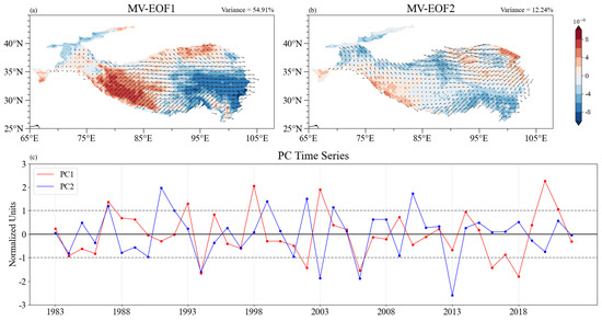
Figure 2.
The spatial pattern of (a) the first and (b) second modes obtained and (c) the PC time series using Combined-EOF of the summer water vapor flux over TP during 1983–2022 (the gray dotted line represents one standard deviation); the filling color represents the water vapor flux divergence, and the vectors represents the water vapor fluxes.
The second mode explains 12.24% of the variance (Figure 2b). During the positive phase, the water vapor flux flows from the southern and northern regions towards the east. The divergence of the water vapor flux exhibits a north–south reverse pattern, with a divergence observed across the whole plateau, although this pattern is not pronounced.
To emphasize the clearly anomalous features, we select positive and negative peak years based on their amplitudes exceeding one standard deviation (Figure 2c). The positive peak years of PC1 are 1987, 1993, 1998, 2003, and 2020, while the negative peak years occur in 1994, 2002, 2006, and 2018. The PC1 time series show a 3–5-year cycle, which is related to the ENSO. The positive peak years of PC2 are 1987, 1991, 1999, 2002, 2004, and 2010, whereas the negative peak years are 1994, 2003, 2006, and 2013.
In fact, by conducting a joint analysis of the longitudinal and latitudinal components of the vertical integral of water vapor, we can obtain two main modes. In the first mode, the moisture flux convergence over the plateau shows an east–west dipole variation type, while the second mode roughly shows a north–south dipole variation type, but not significantly.
3.2. Regression Results for Principal Modes of Water Vapor Fluxes
Water vapor plays a critical role in precipitation formation. To understand the associated relationship, we calculate the regression of water vapor flux to the precipitation field. For the first mode (Figure 3a), anomalous precipitation is enhanced in the southeastern region of the TP due to a convergence system, while a divergence system in the southwest leads to a smaller precipitation anomaly. In addition, precipitation is significantly greater in the Bay of Bengal, and anomalies in the precipitation are reduced in the subtropical zone and the WNPSH. In the southeast of the TP, moisture transport of the precipitation center primarily originates from the South China Sea, the Bay of Bengal, and surrounding areas. The convergence of the water vapor flux in eastern region results in abnormally high precipitation. Miao et al. [46] suggested that the key factor driving precipitation in the southeastern TP during the summer is the long-distance moisture transport from the low-latitude oceans, indicating the TP as an important transfer station in the water cycle.
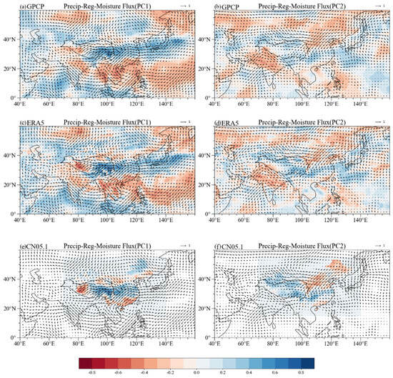
Figure 3.
Distribution of regression coefficients for (a) PC1 and (b) PC2 with precipitation field (color-filled; unit: mm/day), with white dotted area dots representing regression coefficients for shaded area passed 0.05 significance level, and arrows representing primary modes of moisture fluxes from 1983 to 2022 and (c) PC1 and (d) PC2 with precipitation field (color-filled; unit: mm/day) by monthly precipitation field data from ERA5 reanalysis and (e) PC1 and (f) PC2 with precipitation field (color-filled; unit: mm/day) by monthly precipitation field data from CN05.1 (daily meteorological datasets with horizontal resolution of 0.25° × 0.25° interpolated from observations at several stations in China and processed to monthly averages).
In the second mode (Figure 3b), moisture transport over the Indian Peninsula and surrounding regions exhibits a divergence circulation, leading to abnormally low precipitation in the Indus Plain, the Indian Peninsula, and other nearby plains. In the corresponding water vapor flux field, a portion of the moisture enters the TP from the northeast and exits towards the northwest. Additionally, some of the water vapor from the Indian Peninsula bypasses the southern boundary of the plateau and outflows to the southwest, corresponding to the negative precipitation anomaly in the Indian Peninsula.
In fact, we also conducted regression analyses using both ERA5 monthly mean precipitation data (Figure 3c and Figure 3d) and processed CN05.1 monthly mean observation data (Figure 3e and Figure 3f), both with a horizontal resolution of 0.25 × 0.25°. The CN05.1 dataset was constructed for the purpose of high resolution climate model validation over the China region. The dataset is based on the interpolation from over 2400 observing stations in China, interpolated by the anomaly approach. The processed CN05.1 dataset is based on the daily CN05.1 dataset [47]. Firstly, we did not use ERA5 data because it is reanalyzed data with significant errors and it is category D data. On the other hand, GPCP data are widely used, recognized internationally, and are mainly based on observations, so GPCP data were chosen. Secondly, we mainly explore the mode information of large-scale spatial distribution of the TP and surroundings, and search for the slow variable information of the interannual variability of the precipitation field. Comparing Figure 3a and Figure 3b, Figure 3c and Figure 3d, and Figure 3e and Figure 3f, it can be seen that, for the spatial distribution of precipitation field on the TP in summer, Figure 3a, Figure 3c and Figure 3e are of the east–west dipole distribution type, and the spatial distributions of the Figure 3b, Figure 3d and Figure 3f are basically the same. For the large-scale spatial distribution, the spatial distribution mode information in Figure 3a and Figure 3b, Figure 3c and Figure 3d, and Figure 3e and Figure 3f is basically the same. It proves that the GPCP data can fully characterize the large-scale spatial distribution of the precipitation field despite its low resolution. Although the CN05.1 data have higher resolution and the observation data of the TP may be more comprehensive, we did not choose the CN05.1 data in the end, considering the factors as above.
Thermal dynamics has an important influence on large-scale circulation patterns, and understanding the specific mechanisms of dynamic influence has been an important subject of research. Jia et al. [48] pointed out that there is a good negative correlation between OLR and precipitation over the TP in the rainy season. Liu et al. [49] analyzed the characteristics of OLR and precipitation in the rainy season on the eastern TP and found that the center of the high precipitation values basically coincides with the center of the low OLR values, with an inverse correlation in terms of temporal changes. Figure 4 shows the results of the OLR field regression to PCs. By comparing the results of the precipitation field and the OLR field in Figure 3 and Figure 4, it reveals that the center of heavy precipitation closely aligns with the center of convective activity over the TP during the summer.
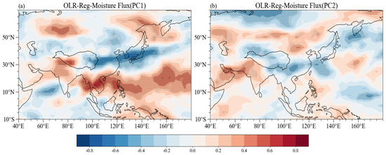
Figure 4.
Distribution of regression coefficients for (a) PC1 and (b) PC2 with OLR field (filled colors; unit: ), with black dotted area indicating that regression coefficients for this shaded area pass 0.01 level of significance, gray color indicating 0.05 level of significance, and light gray color indicating 0.1 level of significance.
In the first mode (Figure 4a), in contrast to Figure 3a, the precipitation anomaly is more in the southeast of the TP, while the atmospheric heating anomalies are less significant and extend to the eastern part of China, Japan, and coastal areas. In this region, the latent heat released from precipitation leads to a reduction in atmospheric heating anomalies. In the southwest, there are fewer precipitation anomalies and higher atmospheric heating anomalies, which extend into the southwestern areas. In addition, atmospheric heating in the Bay of Bengal region is abnormally low, whereas it is significantly higher in the subtropical region. These regression results demonstrate a good correspondence between the precipitation and OLR fields. This indicates that the low-latitude oceanic regions on the south of the plateau, including the South China Sea, the Bay of Bengal, and the tropical Pacific Ocean, as well as the southwestern region of the plateau and the Indian Peninsula, have anomalously high convective activity.
In the second mode (Figure 4b), the atmospheric heating anomalies are abnormally high in the Indus Plain and surrounding regions, while the southeast region of China, the South China Sea, and the Bering Sea show abnormally low atmospheric heating anomalies.
How does the large-scale circulation background respond to the cooperative interaction of the water vapor flux component over the TP? Figure 5 and Figure 6 show the patterns of the different-level circulation anomalies regressed to PC1 and PC2. At the 200 hPa, there is a high-pressure center, corresponding to the South Asian High (SAH), with an anticyclonic flow. It is worth noting that SAH is farther east than the climatic SAH. There is also a high-pressure center on the north side of the jet stream, but a low-pressure center in the east of China, which corresponds to a cyclonic flow. The moving process of the SAH and the upper-level jet stream can affect the convection activity over the TP. The upper part is a divergent flow related to the SAH that controls the rise and outflow of water vapor [50].
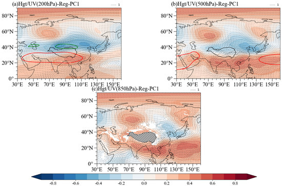
Figure 5.
(a) The 200 hPa, (b) 500 hPa, and (c) 850 hPa circulation anomaly patterns as regressed to PC1 (wind unit: , height unit: ), with the dotted areas passing the significance test at the 95% confidence level, where (a) the green and red contours denote the climatic westerly jet stream and the South Asian High and (b) the red line represents the climatic state of the Western Pacific Sub-High.
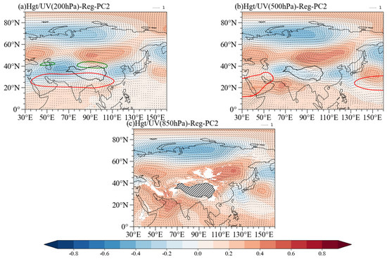
Figure 6.
The same as Figure 5 but for the 200 hPa, 500 hPa, and 850 hPa circulation anomaly patterns as regressed to PC2, where (a) the green and red contours denote the climatic westerly jet stream and the South Asian High and (b) the red line represents the climatic state of the Western Pacific Sub-High.
A high-pressure system is observed on the Indian Peninsula and the South China Sea (Figure 5b), corresponding to the divergence flow field and an anomalous negative precipitation area. Meanwhile, there is a Western Pacific subtropical high-pressure, whose position is significantly farther west than the position of the climatic state (Figure 5b). East China has a low-pressure trough and a northeast cold vortex. The variation in moisture transport at the southern boundary of the TP is closely related to the WNPSH, while moisture transport at the western boundary is mainly influenced by the mid-latitude westerly wind belt.
Influenced by the Indian monsoon (Figure 5c), precipitation patterns in the western and eastern TP exhibit distinct characteristics. The water vapor flux over the Indian Peninsula displays an anomalous cyclonic pattern, with southerly air in the eastern part of the anomaly circulation transporting water vapor from the Bay of Bengal and the South China Sea to the southwestern TP. The strengthening of the westerly flow in the mid-latitudes leads to the transport of water vapor to the southern TP, enhancing the convergence of water vapor centers.
In the second mode, at the 200 hPa (Figure 6a), a high-pressure center is located to the north side of the TP, corresponding to an anticyclonic flow field. On the other hand, there is a low-pressure center on the eastern and western sides of the plateau, corresponding to a cyclonic flow field. At 500 hPa (Figure 6b), the high-pressure center on the northern side of the plateau corresponds to anticyclonic circulation, with a high-pressure center over the Arabian Sea. At the 850 hPa (Figure 6c), the high-pressure system on the northern side of the plateau shifts eastward and weakens, while the high-pressure system over the Arabian Sea strengthens.
Wu et al. [51] found that the surface sensible heating of the TP produced a strong subtropical monsoon meridian circulation, providing the necessary conditions for the development and maintenance of the subtropical monsoon circulation. Similarly to the OLR result, the surface upward is observed to be positive. In the first mode (Figure 7a), when subjected to radiative forcing, the sensible heat flux is less anomalous in the southeastern TP and downstream regions, while it is abnormally high in the southwest and northern TP. The TP acts as a significant heat source during summer, enhancing the local upward movement and intensifying the large-scale SAH in the upper troposphere [9]. During the positive phase, similar to the modal characteristics of the water vapor flux, precipitation field, and OLR field, the sensible heat flux on the Tibetan Plateau shows an east–west dipole variation type. The peripheral areas of the plateau have anomalously high sensible heat fluxes due to the zonal dipole patterns. In the second mode (Figure 7b), the sensible heat flux is abnormally high over large areas of the Indian Peninsula and Indus Plain. This may be due to the meridional pattern.
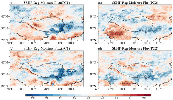
Figure 7.
Sensible heat flux (upper panels) and latent heat flux (lower panels) regressed to PC1 and PC2 (unit:), with black dotted area indicating that regression coefficients for this shaded area pass 0.01 level of significance, gray color indicating 0.05 level of significance, and light gray color indicating 0.1 level of significance.
The latent heat of the TP during summer affects the temperature of the middle and upper troposphere over Central Asia by modulating the plateau monsoon and the Indian Ocean SST. This, in turn, affects the circulation at the 200 hPa and 500 hPa levels, as well as the moisture transport of the whole layer, thus altering precipitation patterns in surrounding regions [52,53]. The analysis considers the surface upward flux to be positive. In the first mode (Figure 7c), the latent heat flux is relatively less anomalous in the southeastern, southwestern, and surrounding areas of the TP, where moisture is released, providing a continuous moisture supply for precipitation. This result is consistent with the precipitation distribution and moisture flux divergence patterns. More moisture is absorbed in the northwestern TP, and the latent heat flux shows a positive correlation with the convective activity in the western TP, which is closely related to the underlying surface characteristics of the western TP [54]. In the second mode (Figure 7d), the latent heat flux is lower in the southwest and southeast of the TP, providing moisture for precipitation in eastern China.
3.3. Influence of SST Anomalies on Moisture Transport over TP
We perform a lead-regression analysis on the pre-winter, pre-spring, and PC time series. The results (Figure 8a) indicate that the SST were abnormally high in the Bohai Sea and the Yellow Sea near eastern China during the previous winter, and in the tropical Indian Ocean. In addition, SST is abnormally high in the equatorial Middle East Pacific and abnormally low in the southern tropical Pacific and the Western Pacific, which are associated with the ENSO. In spring (Figure 8b), SST in the tropical southeast Indian Ocean shows a cold anomaly, while the tropical West Indian Ocean experiences a warm anomaly.
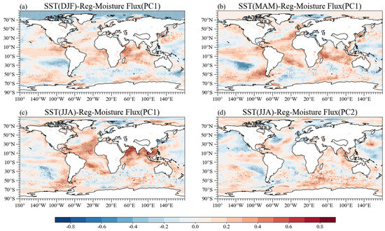
Figure 8.
SST anomaly patterns regressed to PC1 in previous winter and spring (upper panels), and PC1 and PC2 in summer (lower panels, unit: K), with black dotted area indicating that regression coefficients for this shaded area pass 0.01 level of significance, gray color indicating 0.05 level of significance, and light gray color indicating 0.1 level of significance.
SST anomalies affect atmospheric circulation through air–sea interactions. In the first summer mode (Figure 8c), SST is significantly high in the Bay of Bengal, the South China Sea, trans-equatorial region, and South Atlantic. Conversely, SST is significantly low in the South Pacific and the South Indian Ocean, which affects moisture distribution over the TP. In the second mode (Figure 8d), there is a causal relationship between low SST anomalies in the Central Pacific and the northern Atlantic and moisture transport anomalies over the TP.
The Pacific, Indian Ocean, and Atlantic interact separately or cooperatively to influence moisture transport over the TP. This is mainly reflected in the SST anomaly in the Pacific, which is largely driven by ENSO during the previous winter. These anomalies then transmit to the equatorial Indian Ocean and the South China Sea in the spring and summer, affecting summer moisture transport to the TP through the South Asian summer monsoon. Additionally, they affect the IOD and the Indian Ocean Basin during the autumn.
Tao et al. [55] noted that warm SST in the Niño3 region during winter and spring are associated with above-normal precipitation in the south of the Yangtze River in June, as well as a westward displacement of the subtropical high and a southward shift in the summer rain belt. The ENSO event causes abnormal zonal and meridional atmospheric circulation, altering the position and intensity of the atmospheric pressure and wind fields over the TP, which further modifies the heat and moisture transport from ocean to the TP, thus affecting the TP precipitation variations.
We conducted a correlation analysis between Niño3 index in pre-autumn, pre-winter, and pre-spring and PC series in summer (Figure 9a). The Niño3 index of ONO, NDJ, and DJF shows a strong correlation with the PC1 sequence in summer and passed the 95% significance test, indicating that moisture flux over the TP in summer is significantly correlated with the ENSO phenomenon in pre-winter. The conclusion is consistent with the regression results between the SST in pre-winter and the PC sequence. It can be seen that the SST anomaly in the Pacific dominated by ENSO in the pre-winter leads to the abnormal distribution of moisture transporting in the TP in summer.
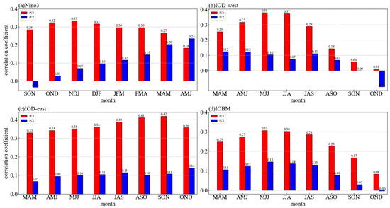
Figure 9.
Lead–Lag correlation analysis among (a) Niño3 index, (b) IOD West Pole index, (c) IOD East Pole index, and (d) IOBM index and PC index, where SST variability factor is sliding mean of 3-month set (abbreviation stands for first letter of each of three consecutive months, e.g., March to May is MAM).
The SST anomalies in the low-latitude ocean on the south side of the plateau play an important role in the water vapor flux over the plateau in summer, so we carry out correlation analysis between IOD West Pole index in pre-spring, summer, and late autumn and PC series in summer (Figure 9b) in order to explore the relationship and influence of water vapor modes over the TP and IOD. The IOD West Pole index of MJJ and JJA shows a strong correlation with the PC1 sequence in summer, which passed the 95% significance test, indicating that the moisture flux over the TP in summer is significantly correlated with the warm pool area of the Indian Ocean. The SST anomalies over the Indian Ocean in summer and the South China Sea led to the abnormal distribution of moisture transporting over the TP in summer. The west pole of IOD has a strong correlation with the moisture transporting over the TP in summer one month ahead.
For the IOD East Pole index (Figure 9c), it can be seen that the IOD East Pole index of MAM, AMJ, MJJ, JJA, JAS, ASO, SON, and OND shows a strong correlation with the PC1 sequencer, which passed the 95% significance test, indicating that the moisture flux over the TP in summer is significantly correlated with the warm pool area of the Indian Ocean. The SST anomalies over the Indian Ocean in summer and the South China Sea will lead to the abnormal distribution of moisture transport over the TP in summer. In addition, the IOD East Pole has a strong correlation with the moisture transport in summer over the TP with a three-month lag, and the IOD East Pole has a strong interaction with the moisture transport over the TP in summer from spring to autumn.
IOBW usually starts to develop in winter and reaches a maximum in the spring of the following year. It has been shown that when an El Niño (La Niña) event develops in the eastern equatorial Pacific Ocean through “atmospheric bridging” [56,57] or the Indian Ocean Nicene through flow [58], the SST in the tropical Indian Ocean shows a regionally consistent warming (cold bias) from winter to the spring and summer of the following year. In the following year, the SST tends to show consistent warming (cooling) across the region. Our study of the IOBM index can further explore the relationship between water vapor fluxes over the TP and air–sea interactions in the Pacific and Indian Ocean. For the IOBM index (Figure 9d), the IOBM index of MJJ and JJA is strongly correlated with the PC1 series, which passed the 95% significance test, indicating that the water vapor flux over the TP in summer is significantly correlated with the IOBM. The conclusion is consistent with the regression of SST in summer and the PC series. It can be seen that the SST anomalies over the Indian Ocean and the South China Sea in summer will lead to the abnormal distribution of moisture transport over the TP in summer. Moreover, IOBM had a strong one-month-ahead correlation with moisture transport over the TP in summer, and the correlation gradually weakened from summer to autumn.
In fact, the effect of the IOD on the summer moisture flux modes of the TP is the most significant with the largest significant regression coefficients. The SST anomalies in this region transport moisture from the equatorial Pacific to the southern part of the TP under the influence of the Indian Summer Wind (ISW), which affects the interannual variability of precipitation in the TP in summer through multiscale moisture convergence. Specifically, when the SST anomalies of the former winter Pacific warm pool are high, the western Pacific sub-height extends westward and strengthens, the Indian summer wind transports a large amount of moisture to the southeastern through the anomalous anticyclonic circulation, and the summer heat source of the plateau pumps the moisture, which makes the moisture convergence transport to the east, and produces the precipitation in the eastern of the TP and in the eastern part of China.
At the same time, we conducted the correlation of EASM and SNAO index to PC2 sequence, however, the correlation is not strong.
4. Discussion
It should be pointed out that the research conclusion of this paper is based on reanalysis data and remote sensing data. Due to the special topography of the TP and the lack of observational data, there are some discrepancies in the different data and errors in the reanalyzed data; other conclusions on the specific region of the TP are not abundant. Through the regression precipitation figures obtained by using different data in Figure 3, it can be seen that although the general spatial distribution is consistent, there are many differences in detail, which also increases our understanding of the differences. These variations provide valuable insights into inter-dataset discrepancies. The reanalyzed data have large error, being class D data, especially at the TP. The areas that passed the significance test of the regression coefficients obtained by reanalyzed data (Figure 3c and Figure 3d) are a little less than the observed data (Figure 3a and Figure 3b). This error could affect our analysis of the results of the distribution of regression coefficients. Among them, only the results of the dotted area are reliable. In this study, we analyze the spatial distribution characteristics of the dotted area and these results are credible.
As mentioned above, several studies have found interactions between ENSO and IOD with specific mechanisms of interaction clearly described [18,19,20,21,22,23,24,25,26,27,59,60,61], and air–sea interactions in the Indian and Pacific Oceans also affect moisture flux in the TP. The mechanism by which the Indian Ocean affects moisture transport to the TP was studied in detail. As shown in Figure 2, the PC1 sequence exhibits a cycle of approximately 3 to 5 years. It is assumed that the main reason for the interannual variability of moisture fluxes comes from the ENSO. However, this study does not explore in detail how the SST anomalies in the Pacific and Indian Oceans act on the moisture flux of the TP. In this study, we research the characteristics of interannual variation in moisture flux on the TP in summer, and only use the correlation coefficient for the SST index, in which there is not much research on the mechanism of the ocean’s action on the TP and the within-seasonal scales. The specific mechanism of SST anomalies on the moisture flux of the TP is not explored by using the method of phase synthesis or the singular value decomposition (SVD) method, by which to obtain the remotely correlated spatial modes features of the SST anomaly field and the main modes field of moisture flux at the TP. It is expected that more intuitive methods will be used to carry out the specific processes underlying these mechanisms in depth. In addition, the SST index of ENSO used in this study is the niño3 index, and the correlation coefficient with the moisture flux of the TP is not very large. So, it can be seen that the SST anomalies in the equatorial Pacific Ocean in the pre-winter can affect the moisture flux of the TP in the summer, but the effect is not very obvious, and the specific reasons for this need to be investigated in depth. We did not apply the wavelet transform method to decompose the multiscale cycle. In the future, it is necessary to refine the mechanism of action and the time scale can be refined by decomposing the multiscale cycle by wavelet transform method.
5. Conclusions
In this study, we used the Combined-EOF analysis of water vapor flux over the TP to obtain the main mode characteristics and regression analysis of water vapor flux divergence, precipitation field, OLR field, SST field, etc. The first two primary interannual modes of the TP summer water vapor fluxes were identified and featured by the zonal and meridional dipole patterns, respectively. In the first mode, there are zonal abnormal fluxes in the water vapor flux over the TP, and SST anomalies over the Pacific Ocean in winter and spring and over the Indian Ocean in summer affected the variation in moisture transporting over the plateau. The main conclusions are as follows:
By making Combined-EOF of the longitude and latitude components of the moisture transporting integral in the TP in summer, we concluded that the spatial distribution of the first mode shows that the water vapor flux is convergent from south, north, and west to east. The divergence integral of water vapor flux presented an east–west inverse phase change.
In the first mode, the divergence integral of water vapor flux presents an east–west reverse change on the TP, and the precipitation, OLR field, and sensible heat flux field also have corresponding variation characteristics. TP is the “transfer station” of water vapor, so there are more precipitation anomalies and fewer OLR anomalies from the east of China to the middle and reaches of the Yangtze River. In the circulation field, the South Asian High at 200 hPa is located to the east of the climatic South Asian High, which affects the moisture convective activity over the TP. The change in moisture transport in the southern boundary of the TP at 500 hPa is closely related to the change in the West Pacific subtropical high. At 850 hPa, under the influence of the Indian monsoon, the precipitation in the west and east of the TP has significantly different characteristics.
In the correlation regression of SST and the SST index, the first mode is related to the SST anomaly in the Pacific dominated by ENSO in pre-winter and the SST anomaly in the tropical Indian Ocean in summer. The SST anomaly in the Pacific Ocean in winter, the Indian Ocean East Pole in summer, the Indian Ocean West Pole, and the Indian Ocean basin in autumn are all related to the first mode of moisture transport over the TP. The Pacific Ocean, the Indian Ocean, and the Atlantic Ocean have a separate or synergistic effect on moisture transport over the TP. The SST anomaly in the Pacific, dominated by ENSO in the previous winter, spreads to the equatorial Indian Ocean and the South China Sea region in spring and summer, affecting the water vapor over the TP in summer through the summer monsoon in South Asia, affecting the Indian Ocean West Pole and Indian Ocean Basin in autumn.
Author Contributions
Conceptualization, H.-L.R. and J.L.; methodology, J.L. and B.C.; software, J.M. and B.C.; validation, H.-L.R., J.L., and J.M.; formal analysis, J.L., H.-L.R., and B.C.; investigation, J.L. and H.-L.R.; writing—original draft preparation, J.L.; writing—review and editing, H.-L.R., J.L., J.M., and B.C.; visualization, J.L.; supervision, H.-L.R., J.M., and B.C.; project administration, H.-L.R.; funding acquisition, H.-L.R. and B.C. All authors have read and agreed to the published version of the manuscript.
Funding
This research was jointly supported by the National Key Research and Development Program of China (Grant number 2023YFC3007503), the Major science and technology project of the Xizang Autonomous Region (Grant No. XZ202402ZD0006), the China National Natural Science Foundation (Grant number 42305044), the Innovation and Development Special Project of China Meteorological Administration (Grant number CXFZ2023J050), the Basic Research and Operational Special Projects (Grant number 2023Z003) of Chinese Academy of Meteorological Sciences.
Data Availability Statement
In this study, the monthly vertical integral of eastward water vapor flux, vertical integral of northward water vapor flux, vertically integrated moisture divergence, geopotential height, zonal/meridional wind, surface sensible heat flux, surface latent heat flux, precipitation and sea surface temperature (SST) were obtained from the ERA5, which can be downloaded from the website at https://cds.climate.copernicus.eu/datasets/reanalysis-era5-single-levels-monthly-means?tab=overview (accessed on 1 March 2025). The OLR data were provided by the NOAA, which can be obtained from the website at https://www.ncei.noaa.gov/products/climate-data-records/outgoing-longwave-radiation-monthly (accessed on 1 July 2024). The monthly precipitation data were provided by the Global Precipitation Climatology Project, downloaded from the website at https://climatedataguide.ucar.edu/climate-data/gpcp-monthly-global-precipitation-climatology-project (assessed on 5 April 2024). The Niño 3 index is available at https://climatedataguide.ucar.edu/climate-data/nino-sst-indices-nino-12-3-34-4-oni-and-tni (accessed on 18 May 2024). The IOD index is available at https://psl.noaa.gov/data/timeseries/month/DS/DMI/ (assessed on 15 April 2024). The IOBM index is available at http://cmdp.ncc-cma.net/Monitoring/cn_nino_index.php?product=cn_nino_index_iobw (accessed on 18 May 2024).
Acknowledgments
We really appreciate NOAA, NCAR, ERA5 and National Weather Information Center for providing the long-term time series datasets. We also thank the National Climate Centre of China Meteorological Administration for providing the IOBM index.
Conflicts of Interest
The authors declare no conflicts of interest.
References
- Xu, X.-D.; Lu, C.; Shi, X.; Gao, S. World water tower: An atmospheric perspective. Geophys. Res. Lett. 2008, 35, 525–530. [Google Scholar] [CrossRef]
- Immerzeel, W.W.; Van Beek, L.P.; Bierkens, M.F. Climate change will affect the Asian water towers. Science 2010, 328, 1382–1385. [Google Scholar] [CrossRef]
- Bibi, S.; Wang, L.; Li, X.; Zhou, J.; Chen, D.; Yao, T. Climatic and associated cryospheric, biospheric, and hydrological changes on the Tibetan Plateau: A review. Int. J. Climatol. 2018, 38, 1–17. [Google Scholar] [CrossRef]
- Wu, S.; Yin, Y.; Zheng, D.; Yang, Q. Climatic trends over the Tibetan Plateau during 1971–2000. J. Geogr. Sci. 2007, 17, 141–151. [Google Scholar] [CrossRef]
- Xu, X.-D.; Zhao, T.-L.; Lu, C.; Shi, X.H. Characteristics of atmospheric water cycle over the Tibetan Plateau. J. Meteor. 2014, 72, 1079–1095. [Google Scholar]
- Feng, L.; Zhou, T. Water vapor transport for summer precipitation over the Tibetan Plateau: Multidata set analysis. J. Geophys. Res.-Atmos. 2012, 117, 85–99. [Google Scholar] [CrossRef]
- Zhou, S.; Wang, P.; Chuan, H.; Wang, C.; Han, J. Spatial distribution of atmospheric water vapor and its relationship with precipitation in summer over the Tibetan Plateau. J. Geog. Sci. 2012, 22, 795–809. [Google Scholar] [CrossRef]
- Liu, G.; Zhao, P.; Nan, S.L.; Chen, J.M.; Wang, H.M. Advances in the study of linkage between the Tibetan Plateau thermal anomaly and atmospheric circulations over its upstream and downstream regions. Acta Meteorol. Sin. 2018, 76, 861–869. [Google Scholar]
- Zhao, P.; Xu, X.; Chen, F.; Guo, X.; Zheng, X.; Liu, L.; Hong, Y.; Li, Y.; La, Z.; Peng, H.; et al. The third atmospheric scientific experiment for understanding the earth-atmosphere coupled system over the Tibetan Plateau and its effects. B Am. Meteorol. Soc. 2018, 99, 757–776. [Google Scholar] [CrossRef]
- Zhao, P.; Chen, L.X. Climatic characteristics of atmospheric heat sources over the Tibetan Plateau and their relationship with precipitation in China over the past 35 years. Sci. China (Ser. D) 2001, 31, 327–332. [Google Scholar]
- Liu, J.-C. Characteristics of Changes in Heat Sources and Water Vapour Sinks on the Tibetan Plateau and Their Influencing Factors. Ph.D. Thesis, Lanzhou University, Lanzhou, China, 2021. [Google Scholar]
- Zhuo, G.; Xu, X.; Chen, L. Water feature of summer precipitation on Tibetan Plateau. Sci. Meteor. Sin. 2002, 22, 1–7. [Google Scholar]
- Gao, D.-Y.; Zou, H.; Wang, W. Effect of water vapor channel on precipitation in Yarlung Zangbo River. J. Mt. Sci.-Engl. 1985, 4, 239–249. (In Chinese) [Google Scholar]
- Meng, D.-L. Observation-Based Study of Summer Water Vapour Transport on the Tibetan Plateau in Relation to Indo-Pacific Warm Pool Processes. Ph.D. Thesis, University of Chinese Academy of Sciences (Institute of Space Information Innovation, Chinese Academy of Sciences), Beijing, China, 2022. [Google Scholar]
- Zhou, T.-J.; Gao, J.; Zhao, Y.; Zhang, L.; Zhang, W. Water vapour transport processes affecting the ‘Asian water tower’. Proc. Natl. Acad. Sci. USA 2019, 34, 1210–1219. [Google Scholar]
- Lin, H.; You, Q.; Jiao, Y.; Min, J.Z. Spatial and temporal characteristics of the precipitation over the Tibetan Plateau from 1961 to 2010 based on high resolution grid-observation dataset. J. Nat. Rsrc. 2015, 30, 271–281. [Google Scholar]
- Liu, H.; Duan, K. Effects of North Atlantic Oscillation on summer precipitation over the Tibetan Plateau. J. Glaciol. Geocryol. 2012, 34, 311–318. [Google Scholar]
- Hu, S.; Zhou, T.; Wu, B. Impact of developing ENSO on the Tibetan Plateau summer rainfall. J. Clim. 2021, 34, 3385–3400. [Google Scholar] [CrossRef]
- Hu, S.; Zhou, T. Skillful prediction of summer rainfall in the Tibetan Plateau on multiyear time scales. Sci. Adv. 2021, 7, eabf9395. [Google Scholar] [CrossRef]
- Zhao, Y.; Zhou, T.; Li, P.; Furtado, K.; Zou, L. Added value of a Convection Permitting Model in simulating Atmospheric Water cycle over the Asian Water Tower. J. Geophys. Res.-Atmos. 2021, 126, e2021JD034788. [Google Scholar] [CrossRef]
- Zhao, Y.; Zhou, T. Interannual variability of precipitation recycle ratio over the Tibetan Plateau. J. Geophys. Res.-Atmos. 2021, 126, e2020JD033733. [Google Scholar] [CrossRef]
- Han, T.-T.; He, S.-P.; Hao, X.; Wang, H.-J. Recent interdecadal shift in the relationship between Northeast China’s winter precipitation and the North Atlantic and Indian Oceans. Clim. Dyn. 2018, 50, 1413–1424. [Google Scholar]
- Jiang, X.; Ting, M. A dipole pattern of summertime rainfall across the Indian subcontinent and the Tibetan Plateau. J. Clim. 2017, 30, 9607–9620. [Google Scholar] [CrossRef]
- Ratna, S.B.; Cherchi, A.; Joseph, P.V.; Behera, S.K.; Abish, B.; Masina, S. Moisture variability over the Indo-Pacific region and its influence on the Indian summer monsoon rainfall. Clim. Dyn. 2016, 46, 949–965. [Google Scholar] [CrossRef]
- Zou, M.; Qiao, S.-B.; Wu, Y.-P.; Feng, G.L. Effect of water vapor transport anomalies in the Tropical Indo-Western Pacific Ocean on summer precipitation in Eastern China. Atmos. Sci. 2017, 41, 988–998. [Google Scholar]
- Zuo, T.; Chen, J.-N.; Wang, H.-N. Variation of regional heat flux in the Western Pacific Warm pool and its relationship with the South China Sea summer monsoon. J. Marine Sci. 2012, 30, 5–13. [Google Scholar]
- Zhang, P.; Chen, B.-H.; Mao, X.-L. Remote correlation between precipitation and Indian Ocean SST over the eastern Tibetan Plateau. Plateau Mt. Meteor. Res. 2008, 2, 15–21. (In Chinese) [Google Scholar]
- Yuan, Y.; Ding, T.; Gao, H.; Li, W. Main modal characteristics of midsummer air temperature in South China and its relationship with SST anomaly. Chin. J. Atmos. Sci. 2018, 42, 1245–1262. (In Chinese) [Google Scholar]
- Chen, J.-N. Characteristics of Heat Flux Variation and Climate Effect at the Air-Sea Interface in Asia Pacific; China Ocean Press: Beijing, China, 2013. [Google Scholar]
- Hu, J.; Duan, A. Relative contributions of the Tibetan Plateau thermal forcing and the Indian Ocean Sea surface temperature basin mode to the interannual variability of the East Asian summer monsoon. Clim Dyn. 2015, 45, 2697–2711. [Google Scholar] [CrossRef]
- Hoell, A.; Funk, C. Indo-Pacific sea surface temperature influences on failed consecutive rainy seasons over eastern Africa. Clim. Dyn. 2014, 43, 1645–1660. [Google Scholar] [CrossRef]
- Chen, X.; You, Q. Effect of Indian Ocean SST on Tibetan Plateau precipitation in the early rainy season. J. Clim. 2017, 30, 8973–8985. [Google Scholar] [CrossRef]
- Chu, C.; Yang, X.Q.; Sun, X.; Yang, D.; Jiang, Y.; Feng, T.; Liang, J. Effect of the tropical Pacific and Indian Ocean warming since the late 1970s on wintertime Northern Hemispheric atmospheric circulation and East Asian climate interdecadal changes. Clim. Dyn. 2018, 50, 3031–3048. [Google Scholar] [CrossRef]
- Yang, X.; Yao, T.; Zhao, H.; Xu, B. Possible ENSO influences on the northwestern Tibetan Plateau revealed by annually resolved ice core records. J. Geophys. Res.-Atmos. 2018, 123, 3857–3870. [Google Scholar] [CrossRef]
- Zhang, B.-B.; Guan, Z.-Y.; Zhang, M.-M. Interdecadal changes in the interannual variation of convective activity in the tropical Northwest Pacific Ocean and the Southeast Indian Ocean. J. Atmos. Sci. 2018, 41, 753–761. (In Chinese) [Google Scholar]
- Wen, Q.; Yang, H. Investigating the role of the Tibetan Plateau in the formation of Pacific meridional overturning circulation. J. Clim. 2020, 33, 3603–3617. [Google Scholar] [CrossRef]
- Yue, S.; Wang, B.; Yang, K.; Xie, Z.; Lu, H.; He, J. Mechanisms of the decadal variability of monsoon rainfall in the southern Tibetan Plateau. Environ. Res. Lett. 2020, 16, 014011. [Google Scholar] [CrossRef]
- Kang, S.F.; Wu, J.M. Climatic characteristics of OLR field over the Tibetan Plateau. Air Image Takahara 1990, 9, 98–103. (In Chinese) [Google Scholar]
- Lorenz, E.N. Empirical Orthogonal Functions and Statistical Weather Prediction; Sci. Rept. No.1.; M. I. T. Department of Meteorology: Cambridge, UK, 1956. [Google Scholar]
- Kutzbach, J.E. Empirical eigenvectors of sea-level pressure, surface temperature and precipitation complexes over North America. J. Appl. Meteorol. 1967, 6, 791–802. [Google Scholar] [CrossRef]
- Preisendorfer, R.W.; Curtis, D.M. Principal Component Analysis in Meteorology and Oceanography; Elsevier: New York, NY, USA, 1988. [Google Scholar]
- Fukumori, I.; Wunsch, C. Efficient representation of the North Atlantic hydrographic and chemical distributions. Prog. Oceanogr. 1991, 27, 111–195. [Google Scholar] [CrossRef]
- De Mey, P.; Benkiran, M. A Multivariate Reduced-order Optimal Interpolation Method and its Application to the Mediterranean Basin-scale Circulation. In Ocean Forecasting; Pinardi, N., Woods, J., Eds.; Springer: Berlin/Heidelberg, Germany, 2002. [Google Scholar] [CrossRef]
- Wang, B. The Vertical Structure and Development of the ENSO Anomaly Mode during 1979–1989. J. Atmos. Sci. 1992, 49, 698–712. [Google Scholar] [CrossRef]
- Sparnocchia, S.; Pinardi, N.; Demirov, E. Multivariate Empirical Orthogonal Function analysis of the upper thermocline structure of Mediterranean Sea from observations and model simulations. Ann. Geophys. 2003, 21, 167–187. [Google Scholar] [CrossRef]
- Miao, Q.-J.; Xu, X.-D.; Zhang, S.-J. Characteristics of the “transition” between the water vapor balance in the Yangtze River Basin and the water vapor transport component in the plateau. J. Meteor. 2005, 1, 93–99. [Google Scholar]
- Wu, J.; Gao, X.-J. A gridded daily observation dataset over China region and comparison with the other datasets. Chin. J. Geophys. 2013, 56, 1102–1111. (In Chinese) [Google Scholar]
- Jia, L.; Zhou, S.-W. Differences in OLR distribution of summer drought and flood years on the Tibetan Plateau. J. Appl. Meteorol. 2002, 13, 371–376. [Google Scholar]
- Liu, M.; Li, D.-L. Characteristics and correlation analysis of OLR and precipitation changes in the rainy season over the eastern Tibetan Plateau. Plateau Meteor. 2007, 26, 249–256. (In Chinese) [Google Scholar]
- Bothe, O.; Fraedrich, K.; Zhu, X. Tibetan Plateau summer precipitation: Covariability with circulation indices. Theor. Appl. Climatol. 2012, 108, 293–300. [Google Scholar] [CrossRef]
- Wu, G.; He, B.; Duan, A.; Liu, Y.; Yu, W. Formation and variation of the atmospheric heat source over the Tibetan Plateau and its climate effects. Adv. Atmos. Sci. 2017, 34, 1169–1184. [Google Scholar] [CrossRef]
- Wang, T.J.; Zhao, Y. Comparative analysis of five sets of surface sensible heat flux data over the Tibetan Plateau in May. J. Meteor. Sci. 2020, 40, 819–828. (In Chinese) [Google Scholar]
- Liebmann, B.; Smith, C.A. Description of a complete (interpolated) outgoing longwave radiation dataset. Bull. Am. Meteor. Soc. 1996, 77, 1275–1277. [Google Scholar]
- Liu, Q.-H.; Yao, X.-P.; Chen, M.-C. Convective activity over the Tibetan Plateau based on OLR data. Chinese J. Atmos. Sci. 2019, 45, 456–470. (In Chinese) [Google Scholar]
- Tao, Y.-W.; Sun, Z.-B.; Li, W.-J.; Li, W.P.; Zuo, J.Q. Relationships Between ENSO and Qinghai-Tibetan Plateau Snow Depth and Their Influences on Summer Rainfall Anomalies in China. Meteorol. Mon. 2011, 37, 919–928. [Google Scholar]
- Klein, S.A.; Soden, B.J.; Lau, N.C. Remote sea surface temperature variations during ENSO: Evidence for a tropical atmospheric bridge. J. Clim. 1999, 12, 917–932. [Google Scholar] [CrossRef]
- Lau, N.C.; Nath, M.J. Impact of ENSO on the variability of the Asian-Australian monsoons as simulated in GCM experiments. J. Clim. 2000, 13, 4287–4309. [Google Scholar] [CrossRef]
- Meyers, G. Variation of Indonesian throughflow and El Niño/Southern Oscillation. Geophys. Res. 1996, 101, 12255–12263. [Google Scholar] [CrossRef]
- Liu, W.; Wang, L.; Chen, D.; Tu, K.; Ruan, C.; Hu, Z. Large-scale circulation classification and its links to observed precipitation in the eastern and central Tibetan Plateau. Clim. Dyn. 2015, 46, 3481–3497. [Google Scholar] [CrossRef]
- Xu, X.-D.; Dong, L.-L.; Zhao, Y.; Wang, Y.J. Effect of “Asian Water Tower” and characteristics of atmospheric water cycle over the Tibetan Plateau. Chin. Sci. Bull. 2019, 64, 2830–2841. [Google Scholar]
- Crétat, J.; Terray, P.; Masson, S.; Sooraj, K.P.; Roxy, M.K. Indian Ocean and Indian summer monsoon: Relationships without ENSO in ocean–atmosphere coupled simulations. Clim. Dyn. 2017, 49, 1429–1448. [Google Scholar] [CrossRef]
Disclaimer/Publisher’s Note: The statements, opinions and data contained in all publications are solely those of the individual author(s) and contributor(s) and not of MDPI and/or the editor(s). MDPI and/or the editor(s) disclaim responsibility for any injury to people or property resulting from any ideas, methods, instructions or products referred to in the content. |
© 2025 by the authors. Licensee MDPI, Basel, Switzerland. This article is an open access article distributed under the terms and conditions of the Creative Commons Attribution (CC BY) license (https://creativecommons.org/licenses/by/4.0/).