A Spatial–Frequency Combined Transformer for Cloud Removal of Optical Remote Sensing Images

Abstract

Cloud removal is a vital preprocessing step in optical remote sensing images (RSIs), directly enhancing image quality and providing a high-quality data foundation for downstream tasks, such as water body extraction and land cover classification. Existing methods attempt to combine spatial and frequency features for cloud removal, but they rely on shallow feature concatenation or simplistic addition operations, which fail to establish effective cross-domain synergistic mechanisms. These approaches lead to edge blurring and noticeable color distortions. To address this issue, we propose a spatial–frequency collaborative enhancement Transformer network named SFCRFormer, which significantly improves cloud removal performance. The core of SFCRFormer is the spatial–frequency combined Transformer (SFCT) block, which implements cross-domain feature reinforcement through a dual-branch spatial attention (DBSA) module and frequency self-attention (FreSA) module to effectively capture global context information. The DBSA module enhances the representation of spatial features by decoupling spatial-channel dependencies via parallelized feature refinement paths, surpassing the performance of traditional single-branch attention mechanisms in maintaining the overall structure of the image. FreSA leverages fast Fourier transform to convert features into the frequency domain, using frequency differences between object and cloud regions to achieve precise cloud detection and fine-grained removal. In order to further enhance the features extracted by DBSA and FreSA, we design the dual-domain feed-forward network (DDFFN), which effectively improves the detail fidelity of the restored image by multi-scale convolution for local refinement and frequency transformation for global structural optimization. A composite loss function, incorporating Charbonnier loss and Structural Similarity Index (SSIM) loss, is employed to optimize model training and balance pixel-level accuracy with structural fidelity. Experimental evaluations on the public datasets demonstrate that SFCRFormer outperforms state-of-the-art methods across various quantitative metrics, including PSNR and SSIM, while delivering superior visual results.

1. Introduction

Optical remote sensing imagery serves as a critical tool for Earth observation, underpinning numerous applications such as water resource management [1,2], environmental monitoring [3], disaster assessment [4], and urban planning [5]. However, the widespread presence of clouds presents a significant challenge, with statistics from the International Satellite Cloud Climatology Project (ISCCP) indicating that the annual global average cloud coverage is approximately 66% [6]. This pervasive cloud cover significantly degrades the quality and accuracy of information extracted from remote sensing data, impeding its use in various downstream tasks [7,8,9]. Consequently, addressing the removal of clouds and recovering the surface information they obscure has become a crucial research challenge [10].

Traditional cloud removal methods rely on leveraging cloud-free regions within cloudy images to reconstruct obscured areas, employing techniques such as interpolation, filtering, and atmospheric scattering-based approaches [11]. For example, Xia et al. [12] developed a variational interpolation method to address cloud occlusion in MODIS data, generating cloud-free snow-covered area images. Zhang et al. [13] introduced a cokriging interpolation technique that exploits the spatial correlation of adjacent pixels and multitemporal data to restore cloud-obscured pixels in multispectral imagery. Shen et al. [14] proposed a locally adaptive thin cloud removal method using homomorphic filtering, effectively identifying cloud and non-cloud regions in the frequency domain. However, while homomorphic filtering excels in low-frequency cloud removal, it struggles with high-frequency regions. To address this, Yu et al. [15] proposed an improved homomorphic filtering method based on statistical image characteristics, isolating low-frequency cloud information and enhancing filtered images using rough set theory. Despite these advances, traditional methods often suffer from limitations when dealing with complex lighting conditions, high color saturation, or the recovery of high-frequency details, leading to potential image distortion and information loss [16].

With the advent of machine learning, cloud removal has seen significant improvements through the use of models capable of learning cloud characteristics and ground background distributions. Hu et al. [17] proposed a multi-output support vector regression (MSVR) model combined with support vector value contour transformation (SVVCT), enabling the removal of thick cloud cover and prediction of surface information in cloud-obscured areas. Similarly, Tahsin et al. [18] proposed a random forest-based optical cloud pixel recovery (OCPR) method to repair cloud pixels in the spatiotemporal spectral continuum. Wang et al. [19] exploited spatial adjacency and multispectral information, utilizing the nonlinear fitting capabilities of random forests for effective cloud removal and information reconstruction. However, machine learning-based methods often rely on manually designed features, necessitating parameter tuning for specific datasets, which can limit generalization and performance in scenarios with complex cloud coverage.

In recent years, deep learning has emerged as a transformative approach, enabling more robust and automated solutions for cloud removal. Deep learning models exhibit superior feature extraction and scene generalization abilities, adaptively learning from extensive datasets and effectively capturing complex patterns within the data, thereby significantly reducing the dependence on manually engineered features [20,21]. They dynamically optimize their parameters, enabling progressive improvements in performance through continuous data-driven learning. Additionally, these models effectively capture multiscale and multidirectional information in images, generating more realistic and detailed cloud-free results. Cloud removal methods based on deep learning can be categorized into three main approaches: CNN-based methods [22], GAN-based methods [23,24], and Transformer-based methods [25].

CNN-based methods focus on learning complex mappings between cloud-covered and ground-truth data, facilitating the precise identification of cloud-covered areas and restoration of obscured details. For instance, Li et al. [26] proposed an end-to-end deep residual symmetric connection network (RSC-Net) for removing thin clouds from Landsat 8 images. Shao et al. [27] introduced a multi-scale feature-convolutional neural network (MF-CNN) capable of detecting thin clouds, thick clouds, and non-cloud pixels simultaneously. Despite their effectiveness, CNNs are constrained by their local receptive fields, which limit their ability to capture wide-ranging contextual information, potentially leading to the loss of fine details and degraded performance under complex cloud cover scenarios.

GAN-based methods achieve effective cloud removal by utilizing adversarial training, consisting of a generator and a discriminator [28]. The generator learns to produce high-quality cloud-free images, while the discriminator differentiates between real and generated images. Singh et al. [29] proposed Cloud-GAN, which uses cycle-consistency loss to generate high-quality cloud-free images from Sentinel-2 data without requiring paired datasets. Wang et al. [30] proposed a conditional generative adversarial network (GAN) framework for cloud removal tasks, which employs GANs with varying receptive fields to address different cloud layers. However, GANs are often plagued by training instability and issues like mode collapse, which can hinder their reliability in real-world applications.

Transformer-based methods leverage their strong sequence modeling and global context capture capabilities for cloud removal. Christopoulos et al. [31] developed an axial transformer that captures temporal evolution characteristics via axial attention. Xia et al. [32] designed a cloud removal network with multi-head sparse attention and gated feed-forward networks to enhance global feature extraction. While Transformer-based methods show promise, they predominantly focus on spatial features, neglecting the potential of frequency information.

As shown in [33], cloud-covered and cloud-free images exhibit significant differences in frequency. Cloud-free regions typically exhibit rich textures and correspond to high-frequency components, whereas cloud regions are dominated by low-frequency characteristics. Therefore, the model can use this difference to efficiently reconstruct the cloud-covered area. However, the current attention mechanism used in the cloud removal task mainly focuses on the channel and spatial dimensions and pays less attention to the importance of frequency features [34]. This limits the model’s ability to capture and utilize key frequency information in the image. Furthermore, the encoded feature maps extract semantic information such as the structure and texture of the image. At this time, combining frequency transformation can more accurately locate cloud distribution while avoiding the redundancy associated with full-frequency operations on the original image.

Based on this, we propose a novel frequency self-attention (FreSA) module that transforms features from the spatial domain to the frequency domain. By analyzing spectral differences between ground objects and cloud regions, FreSA enhances critical features while suppressing noise. Moreover, existing spatial–frequency methods often combine features through addition or concatenation, failing to capture their interactions effectively. To address this problem, we present a spatial–frequency combined Transformer (SFCT) block to jointly extract and integrate spatial and frequency features, improving cloud region identification and background reconstruction. In order to enhance the ability to extract spatial features, we design a dual-branch spatial attention (DBSA) module to capture the spatial information of the image and the relationship between feature channels through two independent branches. Additionally, we introduce a dual-domain feed-forward network (DDFFN) that effectively extracts and utilizes multi-scale features and frequency information from the features. Building upon these innovations, we propose the spatial–frequency combined Transformer network for cloud removal (SFCRFormer), a network that integrates spatial and frequency information to enhance cloud removal performance. The main contributions of this paper are as follows:

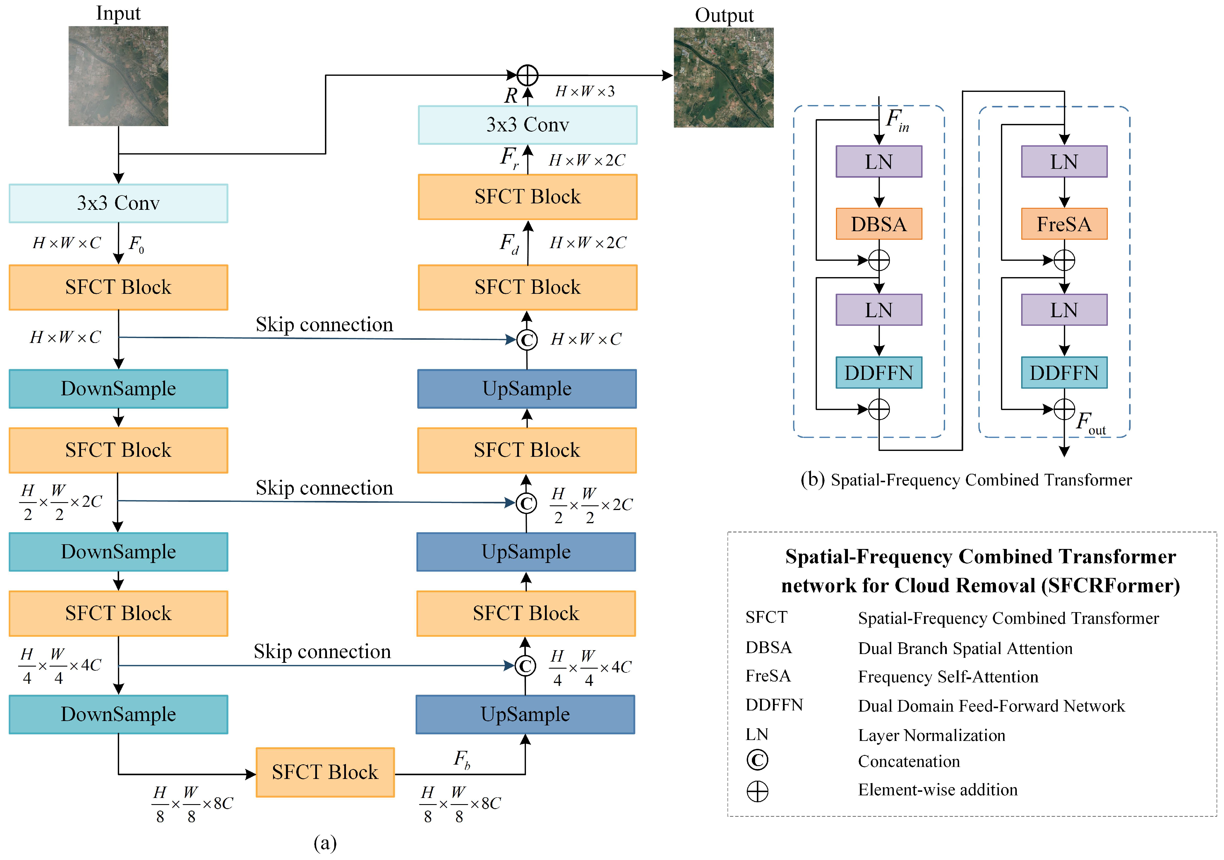
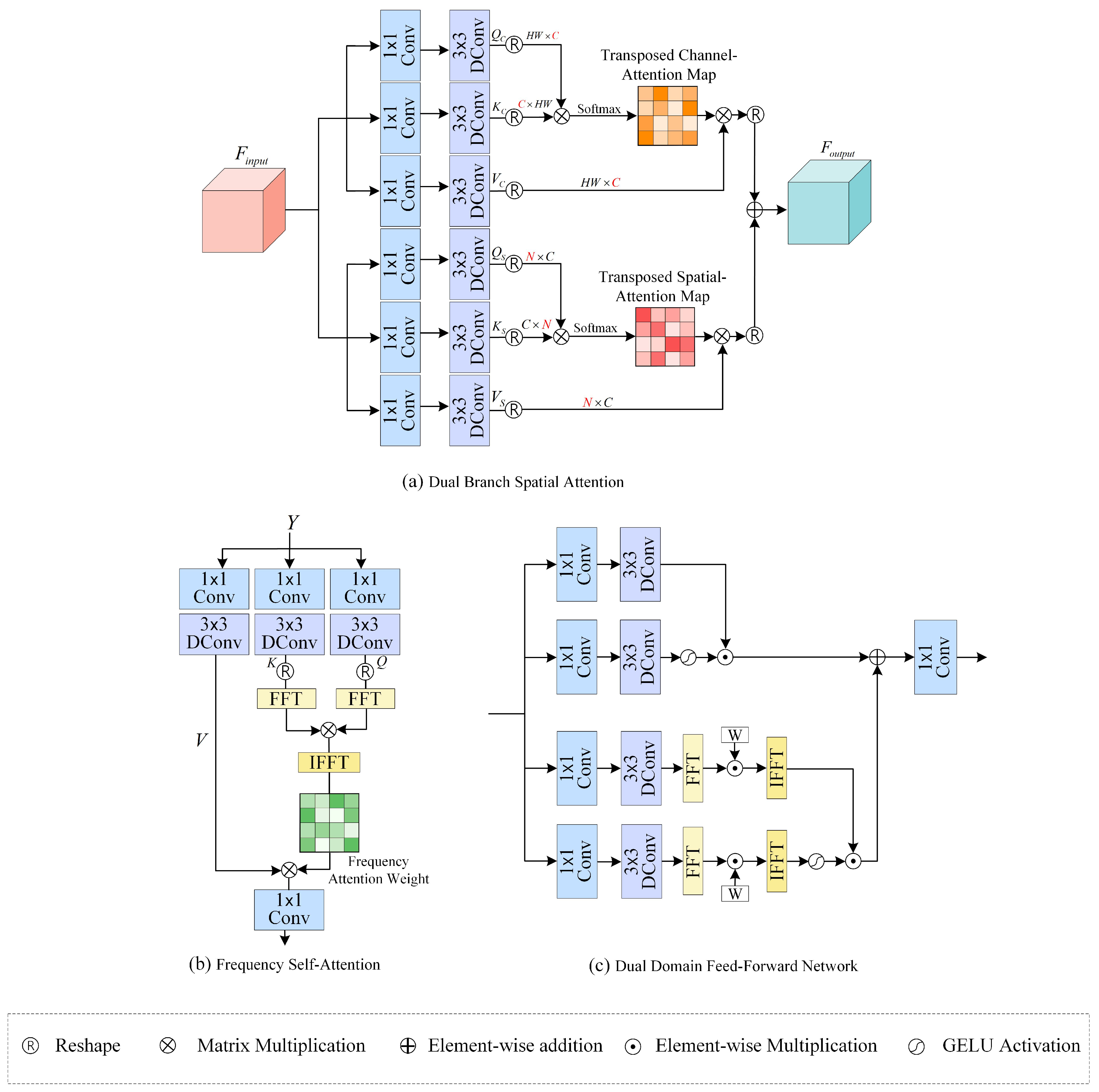
• We present a novel SFCT block, which integrates dual-branch spatial attention (DBSA) and frequency self-attention (FreSA). The DBSA module enhances spatial features by capturing both spatial and channel-wise relationships, effectively addressing structural distortion artifacts inherent in conventional single-branch attention architectures. Meanwhile, the FreSA module operates in the frequency domain, leveraging spectral differences to amplify the contrast between cloud regions and the background, thereby achieving precise detection and comprehensive removal of cloud artifacts.
• We propose the dual-domain feed-forward network (DDFFN) that achieves cloud removal with detail fidelity by capturing pixel-level local textures via multi-scale convolutions and extracting global structural details via frequency transform.
• We design an innovative composite loss function, which integrates the robustness of Charbonnier loss with the perceptual fidelity ensured by SSIM loss. This dual-objective approach not only preserves pixel-level accuracy but also enhances global structural coherence and perceptual quality.
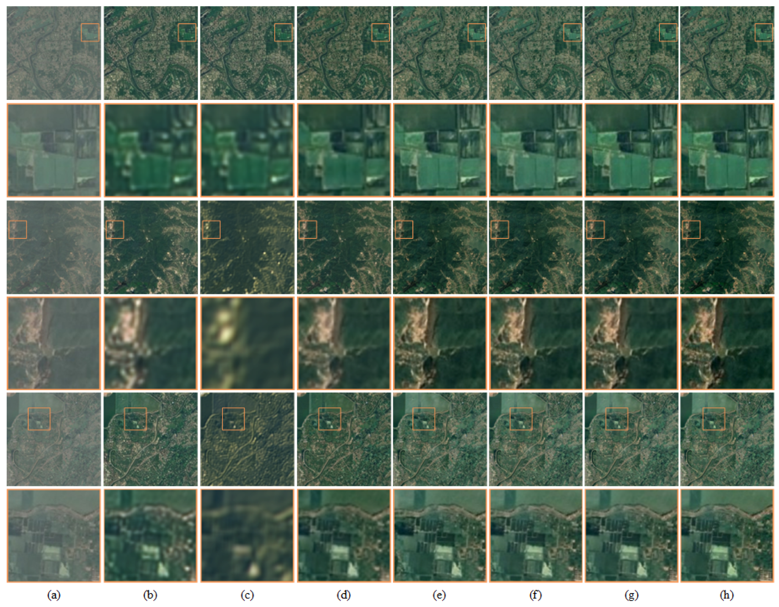
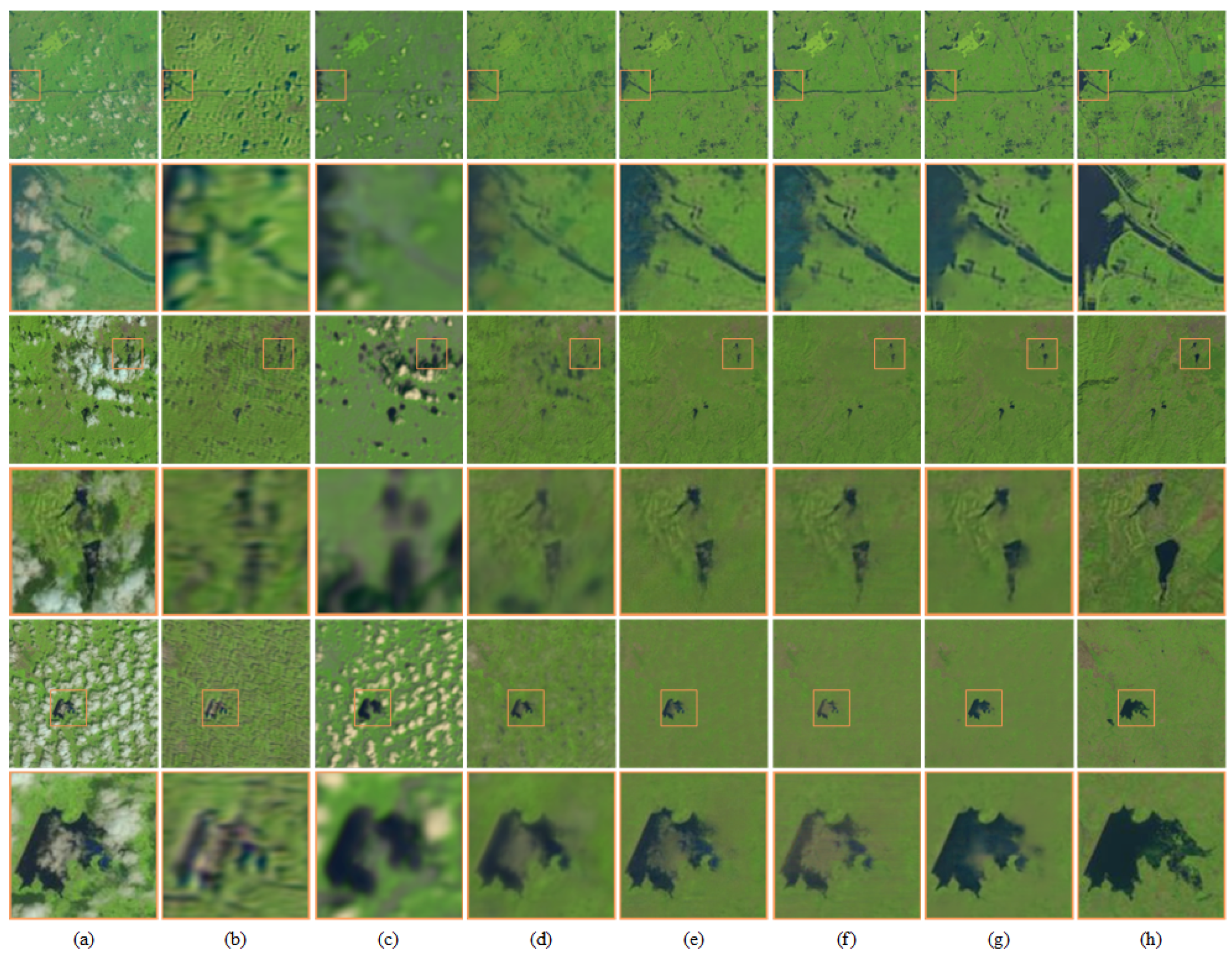
• Extensive experimental validation on multiple benchmark datasets demonstrates that the proposed SFCRFormer significantly outperforms existing state-of-the-art methods in both quantitative metrics and qualitative visual assessments. Our method consistently achieves higher PSNR and SSIM scores, while delivering more visually convincing results, underscoring its robustness and generalization capability across diverse cloud conditions.

2. Related Work

2.1. Deep Learning-Based Cloud Removal Methods

CNNs have been extensively utilized for cloud removal tasks, exploiting their robust feature extraction capabilities to automatically identify and eliminate cloud cover, thus restoring obscured ground information. He et al. [35] developed a lightweight cloud removal network incorporating a deformable context feature pyramid module, enabling adaptive multi-scale feature extraction based on cloud shape and size. Meraner et al. [36] proposed a deep residual neural network architecture that integrates SAR data with optical imagery, improving cloud removal performance through multimodal fusion.

GANs have also gained prominence in cloud removal tasks due to their exceptional capability in generating and restoring realistic cloud-free images, especially in areas heavily obscured by thick clouds. Li et al. [37] introduced the CR-GAN-PM method, integrating GANs with a physical cloud distortion model to decompose cloudy images into cloud/background layers and reconstruct cloud-free results by a refined physical model. Ran et al. [38] developed an end-to-end GAN-based approach incorporating an adaptive padding convolutional activation encoder, which augments boundary feature recognition.

The Transformer architecture, known for its superior sequence modeling and global context comprehension, has recently been adopted in cloud removal research [39]. Zhang et al. [40] proposed a lightweight vision Transformer network for cloud detection, incorporating the dark channel prior to enhance cloud feature extraction. Ge et al. [41] combined Transformers with CNNs, facilitating the simultaneous extraction of local and global features for more accurate cloud identification. Xia et al. [42] proposed a hybrid model that merges Transformers and GANs, which leverages CycleGAN to establish bidirectional mappings between cloudy and cloud-free images and employs Transformer-based modules for long-range dependency modeling. Wang et al. [43] introduced a two-stage cloud removal network where the first stage employs a Swin Transformer for coarse cloud removal, and the second stage utilizes a diffusion model in the latent space to refine details, thereby enhancing the quality of the declouded images. Chi et al. [44] integrated prior information into the Swin Transformer, adaptively extracting and aggregating multi-scale information from each level of the Swin Transformer to reasonably estimate haze parameters and generate dehazed images.

2.2. Applications of Frequency Domain in Remote Sensing

The transformation of data from spatial to frequency facilitates the revelation of periodic characteristics and texture patterns inherent in surface information, thereby improving task-specific outcomes [45]. Hsu et al. [46] employed multi-level wavelet decomposition to separate rain streaks into low-frequency structural and high-frequency detail sub-images and effectively remove low- and high-frequency rain streaks at each level separately from rain images. Guo et al. [47] proposed a cloud perception integrated fast Fourier convolutional network (CP-FFCN) for single remote sensing image cloud removal. This method uses fast Fourier convolution (FFC) to selectively learn the properties of clouds and fog from the frequency domain to remove clouds and reconstruct underlying ground objects.

However, relying solely on frequency domain information may not be sufficient to comprehensively capture all the detailed features of the image. Therefore, many studies have adopted spatial–frequency fusion approaches to more effectively address complex image processing tasks. Zhou et al. [48] proposed an end-to-end joint frequency-spatial domain network (JFSDNet) for remote sensing image change detection. The method uses frequency information to compensate for the loss of image details caused by downsampling, thereby achieving more accurate change region detection. Jiang et al. [49] combined dual-tree complex wavelet transform (DTCWT) and a CNN to improve the cloud removal accuracy through two-stage frequency domain optimization.

Unlike most existing spatial–frequency fusion methods that rely on concatenation or the direct addition of spatial and frequency features, the proposed SFCRFormer first extracts spatial features through the DBSA module, and then transforms these spatial features into the frequency domain via the FreSA module for further refinement. This enables a more effective cross-domain synergy interaction between spatial and frequency information, achieving more precise cloud detection and removal.

3. Method

This section introduces the proposed cloud removal network, SFCRFormer, an advanced architecture that combines spatial and frequency domain features to effectively achieve cloud removal in remote sensing imagery. We first provide an overview of the model’s overall architecture in Section 3.1, followed by detailed descriptions of the proposed modules in Section 3.2, Section 3.3, Section 3.4. Finally, the composite loss function is explained in Section 3.5.

3.1. Overview

The SFCRFormer adopts a U-shaped encoder–decoder structure, as depicted in Figure 1a. Given a cloudy optical image $I\in {\mathbb{R}}^{H\times W\times 3}$, the model first applies a $3\times 3$ convolution to extract shallow features $F_0\in {\mathbb{R}}^{H\times W\times C}$, where H and W denote the image dimensions, and C is the number of feature channels. These shallow features are then processed by the encoder and decoder to extract deep features $F_d\in {\mathbb{R}}^{H\times W\times 2C}$. The deep features $F_d$ are further refined through SFCT block to obtain features $F_r$. The final output feature $F_r$ is processed through a $3\times 3$ convolution to generate a residual image $R\in {\mathbb{R}}^{H\times W\times 3}$. The residual R is then added to the input image I to produce the cloud-free image.

The encoder compresses the input through a series of SFCT blocks, progressively reducing the resolution while capturing long-range dependencies. The decoder reconstructs the feature maps by gradually restoring their resolution, starting from the bottleneck features $F_b\in {\mathbb{R}}^{{\displaystyle \frac{H}{8}}\times {\displaystyle \frac{W}{8}}\times 8C}$. Pixel-unshuffle and pixel-shuffle operations are utilized for efficient downsampling and upsampling, respectively. Skip connections between corresponding encoder and decoder layers are incorporated to preserve fine-grained details.

Unlike traditional Transformers, the SFCT block in SFCRFormer combines a spatial Transformer with a frequency domain Transformer, as shown in Figure 1b. The input feature $F_{in}$ is processed sequentially: The spatial Transformer captures local and global dependencies, while the frequency domain Transformer enhances texture and periodic patterns. This design allows SFCRFormer to effectively model both spatial and frequency features, improving its ability to distinguish cloud regions from ground objects in complex scenes.

3.2. DBSA: Dual-Branch Spatial Attention

The DBSA module integrates spatial and channel attention mechanisms to adaptively handle the variable shapes and positions of clouds. Its structure is shown in Figure 2a. Given an input feature $F_{input}\in {\mathbb{R}}^{\widehat{H}\times \widehat{W}\times \widehat{C}}$, parallel $1\times 1$ point-wise convolutions and $3\times 3$ depth-wise convolutions are applied to generate two sets of $query$, $key$, and $value$ matrices: $Q_c,K_c,$ and $V_c$ and $Q_s,K_s,$ and $V_s$. These operations are defined as follows:

$$\begin{array}{cc}\hfill Q_c=W_d^Q{W}_c^Q{F}_{input},& K_c=W_d^K{W}_c^K{F}_{input},V_c=W_d^V{W}_c^V{F}_{input},\hfill \\ \hfill Q_s=W_d^Q{W}_c^Q{F}_{input},& K_s=W_d^K{W}_c^K{F}_{input},V_s=W_d^V{W}_c^V{F}_{input},\hfill \end{array}$$

(1)

where $W_c^{(·)}$ and $W_d^{(·)}$ represent the weights of point-wise and depth-wise convolutions, respectively. Compared with ordinary convolution, point-wise convolution and depth-wise convolution can reduce computational complexity.

In the channel branch, $Q_c$, $K_c$, and $V_c$ are reshaped into $\left(HW\right)\times C$. The attention map is calculated as follows:

$$\mathrm{ChannelAtt}(Q_c,K_c,V_c)=\mathrm{softmax}\left({\displaystyle \frac{Q_c{K}_c^T}{\alpha }}\right)V_c,$$

(2)

where $\alpha =\sqrt{d}$ scales the dot product for numerical stability.

For the spatial branch, $Q_s$, $K_s$, and $V_s$ are divided into non-overlapping windows of size N, and similar operations yield the spatial attention:

$$\mathrm{SpatialAtt}(Q_s,K_s,V_s)=\mathrm{softmax}\left({\displaystyle \frac{Q_s{K}_s^T}{\alpha }}\right)V_s.$$

(3)

The outputs of both branches are summed element-wise to produce the final DBSA output:

$$F_{out}=\mathrm{ChannelAtt}(Q_c,K_c,V_c)+\mathrm{SpatialAtt}(Q_s,K_s,V_s).$$

(4)

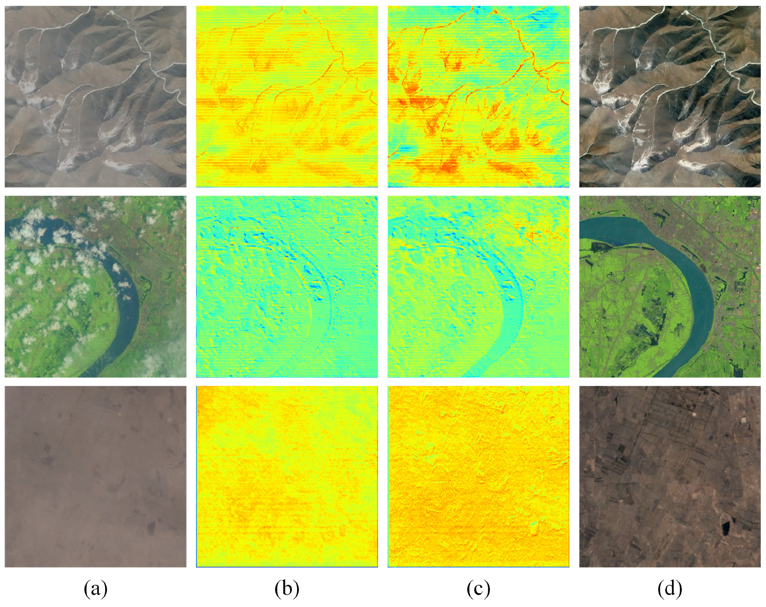
3.3. FreSA: Frequency Self-Attention

The FreSA module leverages the frequency domain to enhance the model’s ability to capture fine details. Its structure is shown in Figure 2b. Given an input $Y\in {\mathbb{R}}^{H\times W\times C}$, we apply $1\times 1$ point-wise convolution and $3\times 3$ depth-wise convolution operations to produce $Q,K,$ and V:

$$Q=W_d^Q{W}_c^{Q}Y,K=W_d^K{W}_c^{K}Y,V=W_d^V{W}_c^{V}Y.$$

(5)

The matrices Q and K are converted to the frequency domain through FFT. Subsequently, their multiplication is followed by IFFT to convert the features back to the spatial domain to obtain the frequency attention weight A:

$$A={\mathcal{F}}^{-1}(\mathcal{F}\left(Q\right)·\mathcal{F}\left(K\right)).$$

(6)

The final frequency attention is derived by weighting V with A and applying a convolution:

$$\mathrm{FreAtt}=\mathrm{Conv}(A·V).$$

(7)

3.4. DDFFN: Dual-Domain Feed-Forward Network

The DDFFN, as shown in Figure 2c, combines spatial and frequency domain branches to comprehensively capture local and global features.

For the spatial branch, we perform convolution operations on the feature in two parallel paths, one of which is activated by the $GeLu$ nonlinear function. The features of the two paths are multiplied to obtain the output of the spatial branch. The formula is

$$\mathrm{SpaFFN}\left(X\right)=\left(W_d^1{W}_c^{1}X\right)\odot \sigma \left(W_d^2{W}_c^{2}X\right),$$

(8)

where ⊙ denotes element-wise multiplication.

For the frequency branch, we convert the features into the frequency domain through FFT to extract information at different frequencies. Moreover, we introduce a frequency component matrix W to adaptively determine which frequency components are retained.

$$\begin{array}{c}{X}_f^1={\mathcal{F}}^{-1}\left(W\left(\mathcal{F}\left(W_c^1{W}_d^{1}X\right)\right)\right),\\ X_f^2={\mathcal{F}}^{-1}\left(W\left(\mathcal{F}\left(W_c^2{W}_d^{2}X\right)\right)\right),\\ \mathrm{FreFFN}\left(X\right)=X_f^1\odot \left(\sigma \left(X_f^2\right)\right).\end{array}$$

(9)

The combined output is

$$\mathrm{DDFFN}\left(X\right)=\mathrm{Conv}\left(\mathrm{SpaFFN}\right(X)+\mathrm{FreFFN}(X\left)\right).$$

(10)

3.5. Loss Function

To balance pixel-level accuracy and perceptual quality, we design a composite loss function, which includes Charbonnier loss $L_c$ [50] and SSIM loss $L_{ssim}$ [51]. The loss function can be defined as

$$L_{total}=L_c+\lambda L_{ssim}.$$

(11)

where $\lambda$ is a hyperparameter, and its value is determined through experimental analysis.

The L1 loss is more robust to outliers but exhibits slower training convergence and may lead to detail loss, while the L2 loss is highly sensitive to noisy data or outliers, resulting in blurry reconstructions. Charbonnier loss combines the advantages of L1 and L2 loss and effectively preserves image details while reducing noise interference during the cloud removal process. It is defined as

$$L_c=\sum _{n=0}^{N-1}\sqrt{{\parallel O_n-G\parallel }^2+{ϵ}^2},$$

(12)

where O is the output of SFCRFormer, and G is the ground truth. $ϵ$ is the constant and is set to ${10}^{-3}$.

Cloud occlusion leads to the loss of texture and structural details of the ground surface. SSIM loss evaluates the structural similarity of images on three aspects, brightness, contrast, and structure, effectively guiding the model to recover clearer edges and finer details while avoiding information loss caused by excessive smoothing. Furthermore, the SSIM loss is more consistent with the evaluation standards of the human visual system, thereby enhancing the visual perceptual quality of the reconstructed images. It is

$$L_{ssim}={\displaystyle \frac{1}{N}}\sum _{n=0}^{N-1}(1-\mathrm{SSIM}(O_n,G)).$$

(13)

4. Experiments

In this section, we introduce the datasets, evaluation metrics, and experimental settings used in the experiments. Then, we present the experimental results on different datasets and conduct ablation studies, while providing a detailed analysis of the findings.

4.1. Datasets

To verify the effectiveness of our proposed method, we conducted a series of experiments on the RICE dataset and the T-Cloud dataset.

4.1.1. RICE Dataset

The RICE dataset [52] contains two subdatasets, namely, RICE1 and RICE2. RICE1 is a thin cloud dataset from Google Earth, including 500 pairs of cloud images and ground truth. RICE2 is a thick cloud dataset from Landsat 8 OLI/TIRS, including 736 pairs of cloud images, ground truth, and cloud mask. The size of the images in both datasets is $512\times 512$. To facilitate model training and evaluation, we partitioned the datasets as follows: 80% of the images are used for training, and the remaining 20% of the images are used for testing. For RICE1, 400 images are used for training and 100 for testing. For RICE2, 589 images are used for training and 147 for testing.

4.1.2. T-Cloud Dataset

T-Cloud [53] is a large-scale thin cloud dataset collected by the Landsat 8 satellite, including 2939 pairs of images with clouds and ground truth. The interval between the acquisition of cloud images and cloud-free images is 16 days. The size of the images in the dataset is $256\times 256$. Similar to the RICE dataset, we use 80% of the images for training and the remaining 20% for testing. That is, 2351 images are used for training and 588 images are used for testing.

4.2. Evaluation Metrics

To evaluate the quality of the restored images, we apply a variety of metrics to quantitatively analyze the experimental results, including peak signal-to-noise ratio (PSNR), Structural Similarity Index Measure (SSIM), mean absolute error (MAE), and root mean squared error (RMSE). The PSNR is an important metric for assessing image reconstruction quality, quantifying the fidelity of the restored image. The SSIM takes into account the luminance, contrast, and structural information of images, evaluating image quality by comparing local structural features between two images, which can more accurately reflect perceived image quality. The MAE assesses image quality by calculating the mean of absolute differences between the pixel values of the reconstructed and ground truth. The RMSE calculates the average of the square roots of the differences between the pixel values of the reconstructed and ground truth. The RMSE is more sensitive to larger errors and is suitable for evaluating significant deviations. Their definitions are as follows:

$$PSNR(x,y)=20lo{g}_{10}\left({\displaystyle \frac{1}{RMSE(x,y)}}\right)$$

(14)

$$SSIM(x,y)={\displaystyle \frac{(2{\mu }_x{\mu }_y+C_1)(2{\sigma }_{xy}+C_2)}{({\mu }_x^2+{\mu }_y^2+C_1)({\sigma }_x^2+{\sigma }_y^2{+}_2)}}$$

(15)

$$MAE={\displaystyle \frac{1}{H\times W}}\sum _{i=1}^H\sum _{j=1}^W\left|x(i,j)-y(i,j)\right|$$

(16)

$$RMSE=\sqrt{{\displaystyle \frac{1}{H\times W}}\sum _{i=1}^H\sum _{j=1}^W{\left(x(i,j)-y(i,j)\right)}^2}$$

(17)

where x and y represent the two images to be evaluated. H and W are the height and width of the images. $x(i,j)$ and $y(i,j)$ represent the pixel value of the image at position $(i,j)$. ${\mu }_x$ and ${\mu }_y$ are the means of images x and y. ${\sigma }_x$ and ${\sigma }_y$ are the standard deviations of images x and y. $C_1$ and $C_2$ are constants.

4.3. Experimental Settings

We implemented the proposed method using the Pytorch framework on an NVIDIA A40 GPU. Our approach uses a four-level encoder–decoder architecture, with the number of SFCT blocks set to [2, 3, 3, 4] at each level, respectively. The number of attention heads in the DBSA is configured as [1, 2, 4, 8]. The channel expansion factor $\gamma$ in DDFFN is set to 0.66. We use the Adam optimizer to optimize the parameters and set the initial learning rate to $2\times {10}^{-4}$. The parameters ${\beta }_1$, ${\beta }_2$ and $ϵ$ are set to 0.9, 0.999 and $1\times {10}^{-8}$, respectively. We trained for 250 epochs with a patch size of $256\times 256$ and a batch size of 2.

4.4. Experimental Results

To verify the effectiveness of the proposed method, in this section, we compare it with five other state-of-the-art methods, including SpA GAN [54], AMGAN [55], CVAE [53], Restormer [56], and TCME [57]. SpA GAN and AMGAN are both GAN-based cloud removal models. Specifically, SpA GAN introduces the spatial attention mechanism into GAN to remove thin clouds from images. AMGAN uses an attentive recurrent network in GAN to extract the distribution of clouds and achieves cloud removal through an attentive residual network. CVAE generates multiple reasonable cloud-free images for each input image through a conditional variational autoencoder. It further refines the output through uncertainty analysis, synthesizing more accurate and clearer images from the multiple predictions generated. Restormer and TCME are both Transformer-based models. TCME enhances the self-attention mechanism in Transformers by incorporating a Top-K sparse selection mechanism, which retains the most informative self-attention values to improve cloud removal performance. Restormer is an image restoration method that has achieved excellent performance in multiple image restoration tasks and is also the baseline of this paper.

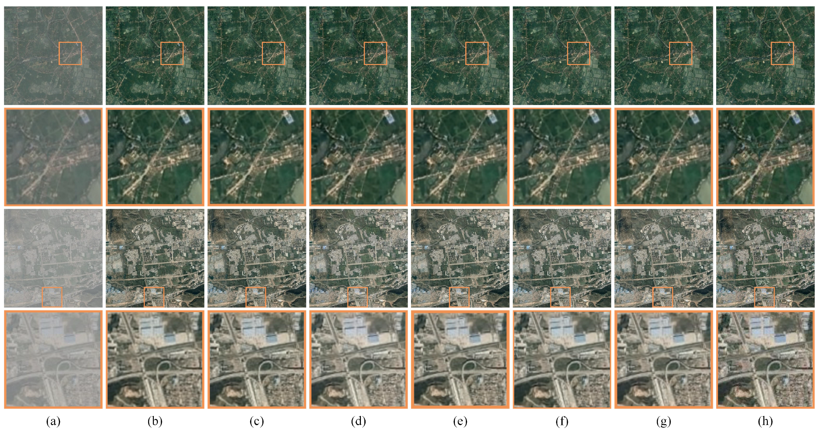
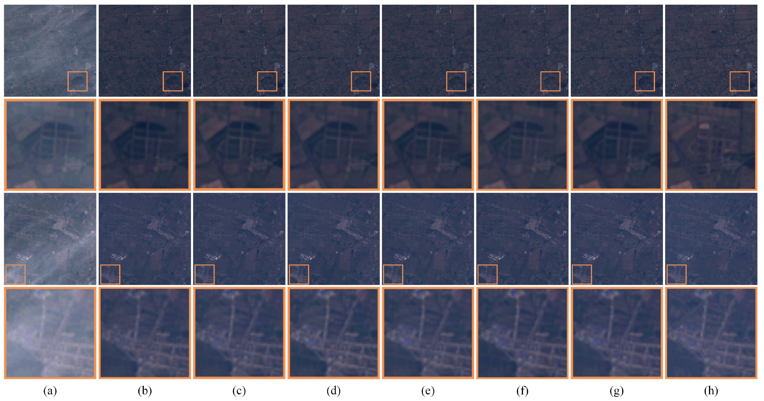
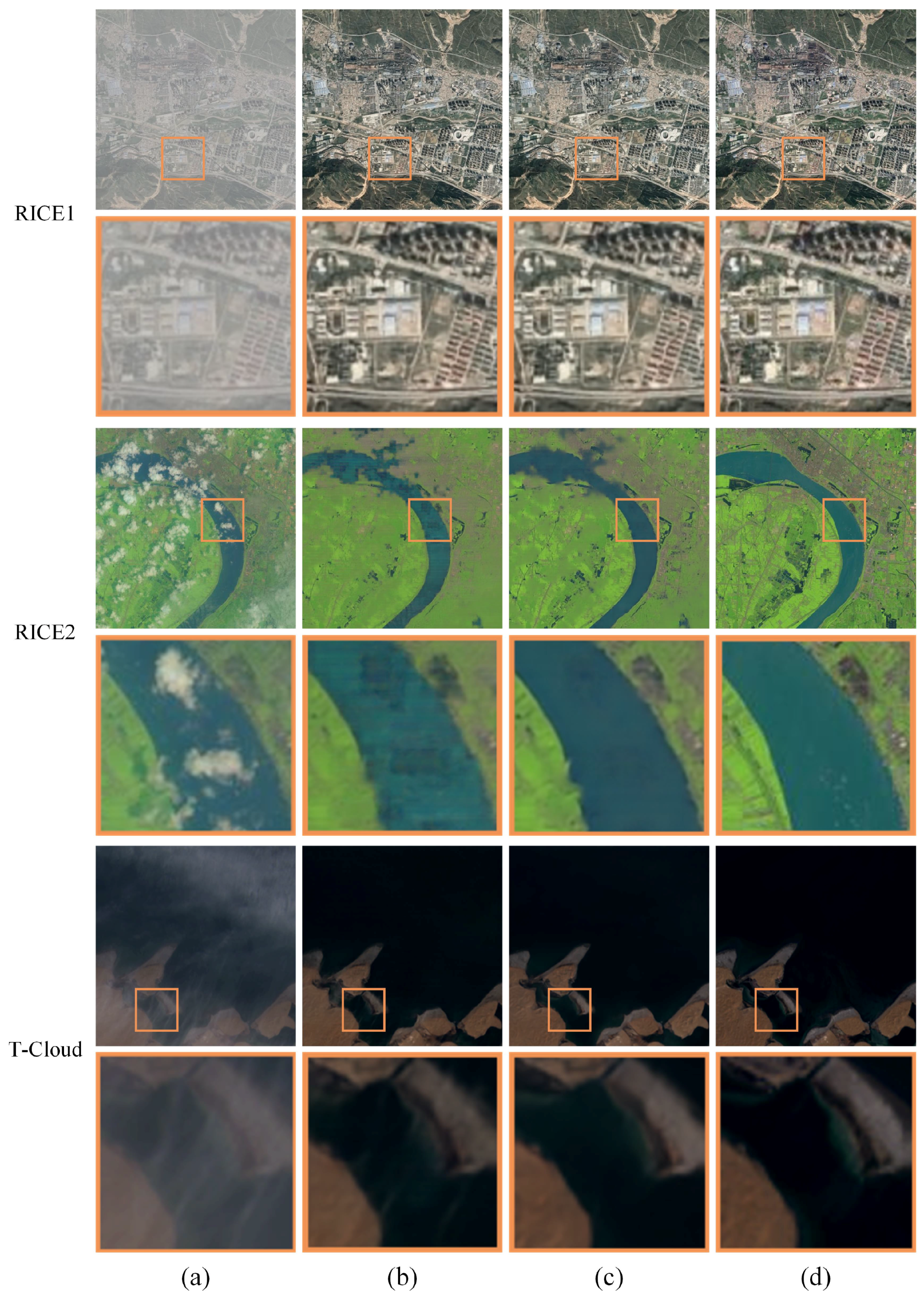
4.4.1. Results on RICE1 Dataset

Table 1. Quantitative results compared with the state-of-the-art methods on the RICE1 dataset, where ↑ indicates higher scores are better, and ↓ indicates lower scores are preferred.

Method	PSNR (↑)	SSIM (↑)	MAE (↓)	RMSE (↓)
SpA GAN	29.5965	0.9165	0.03970	0.05013
AMGAN	25.2576	0.7632	0.06761	0.08374
CVAE	32.1995	0.9485	0.02874	0.03624
Restormer	36.5432	0.9605	0.01786	0.02273
TCME	36.5279	0.9590	0.01806	0.02292
SFCRFormer	37.3512	0.9699	0.01662	0.02064

The underline indicates the second-best result and the bold indicates the best result.

presents the quantitative performance of various state-of-the-art methods on the RICE1 dataset. The best results are highlighted in bold, while the second-best results are underlined. As evidenced by the table, the proposed SFCRFormer consistently outperforms all other methods across the four evaluation metrics, achieving remarkable scores of 37.3512 for PSNR, 0.9699 for SSIM, 0.01662 for MAE, and 0.02064 for RMSE. These results reflect an enhancement of at least 2.2%, 0.98%, 6.9%, and 9.1% over the second-best method, Restormer, in each respective metric. The superior performance of SFCRFormer demonstrates its ability to effectively remove thin clouds while maintaining intricate image details, thus delivering significantly higher image quality. By effectively integrating spatial and frequency domain features, SFCRFormer achieves precise reconstruction and contributes to its robustness across diverse scenes.

Figure 3 presents the visual comparison of different methods on the RICE1 dataset. To facilitate a clearer evaluation, specific regions of the images are magnified to emphasize the cloud removal effects achieved by each approach. The columns in the figure are organized as follows: The first column displays the original cloudy remote sensing images, the second to sixth columns show the results of the comparison methods (SpA GAN, AMGAN, CVAE, Restormer, and TCME), the seventh column depicts the results generated by our proposed SFCRFormer, and the final column provides the ground truth.

From the visual results, it is evident that the two GAN-based methods (SpA GAN and AMGAN) produce blurry images with prominent artifacts and noticeable color distortions. Although CVAE achieves a moderate improvement in image clarity, it still suffers from color distortion and falls significantly short of the quality presented in the ground truth. Transformer-based methods demonstrate a substantial enhancement in both image sharpness and the preservation of spatial details compared to the aforementioned approaches. Among these, Restormer and TCME exhibit superior performance; however, they still struggle to accurately recover fine-grained structural details in cloud-covered areas.

In contrast, our proposed SFCRFormer achieves the most visually compelling results. It not only restores the contour edges of ground objects with remarkable clarity but also reconstructs more accurate detailed features. These results highlight the efficacy of the spatial–frequency domain fusion in SFCRFormer, which effectively balances global structural restoration and local detail preservation.

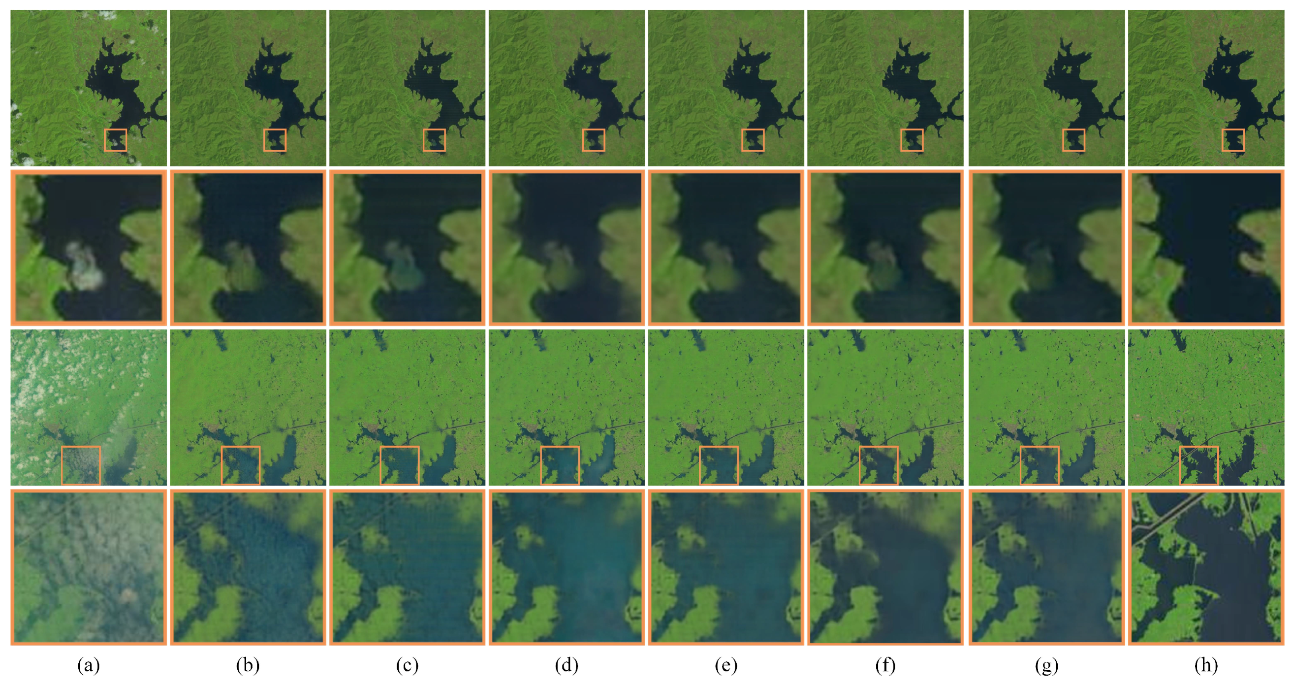
4.4.2. Results on RICE2 Dataset

Table 2. Quantitative results compared with the state-of-the-art methods on the RICE2 dataset, where ↑ indicates higher scores are better, and ↓ indicates lower scores are preferred.

Method	PSNR (↑)	SSIM (↑)	MAE (↓)	RMSE (↓)
SpA GAN	30.0268	0.8244	0.03751	0.04508
AMGAN	27.1915	0.8057	0.05312	0.06705
CVAE	32.3241	0.8566	0.02763	0.03698
Restormer	36.2070	0.9155	0.01884	0.02554
TCME	36.8512	0.9179	0.01871	0.02530
SFCRFormer	37.7584	0.9264	0.01709	0.02339

The underline indicates the second-best result and the bold indicates the best result.

shows the results of various methods on the RICE2 dataset, with the best results highlighted in bold and the second-best results underlined. Compared to the RICE1 dataset, the RICE2 dataset exhibits significantly higher cloud coverage and density, substantially increasing the complexity of cloud-free image reconstruction. Nevertheless, the experimental results demonstrate that our proposed SFCRFormer achieves superior performance relative to other methods, underscoring its effectiveness and robustness even under more challenging conditions.

Figure 4 is the visualization results and their local magnified images of all methods on the RICE2 dataset. Due to the denser cloud coverage in the RICE2 dataset, the details of ground objects are severely occluded, which increases the difficulty of removing cloud layers in the model. As shown in the third and fourth rows of Figure 4, SpA GAN is vulnerable to cloud shadow regions, leading to the generation of numerous dark patches. Similarly, AMGAN, which also employs GAN as its backbone architecture, encounters comparable issues. Specifically, AMGAN struggles to effectively reconstruct cloud-covered regions, and there may even be cloud residues. Although CVAE leverages multiple predictions to generate relatively accurate results, it suffers from significant artifacts during the reconstruction process, resulting in blurred images. Depending on the powerful modeling capabilities of transformers, Restormer and TCME have achieved notable improvements in spatial detail recovery compared to previous approaches. However, from the results in the second and sixth rows of Figure 4, it indicates that both methods exhibit some degree of color distortion and also generate details that do not match the actual surface information.

In contrast, our proposed SFCRFormer effectively leverages contextual information and suppresses noise interference, generating cloud-free images with fewer artifacts, richer details, and higher color fidelity.

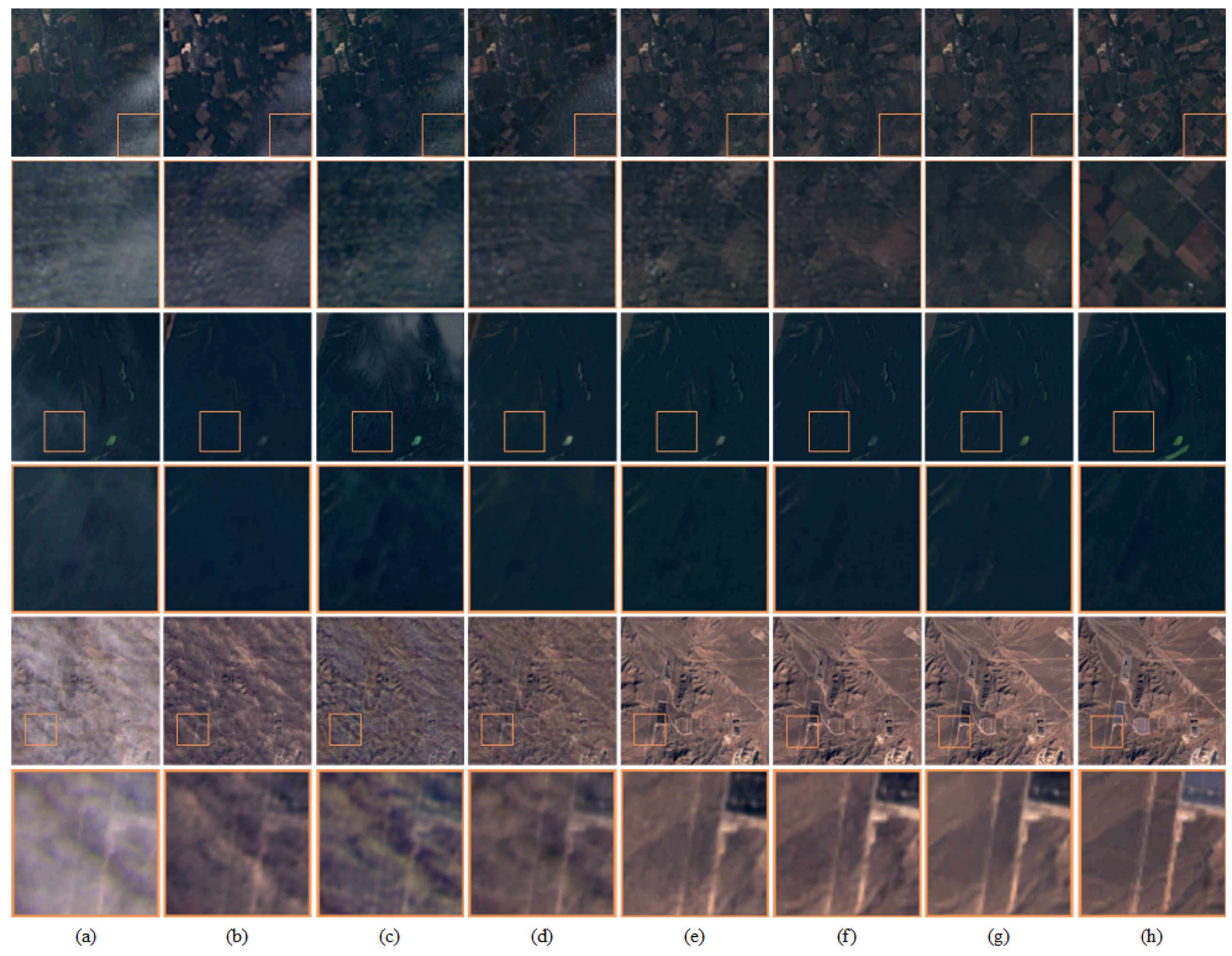
4.4.3. Results on T-Cloud Dataset

Table 3. Quantitative results compared with the state-of-the-art methods on the T-Cloud dataset, where ↑ indicates higher scores are better, and ↓ indicates lower scores are preferred.

Method	PSNR (↑)	SSIM (↑)	MAE (↓)	RMSE (↓)
SpA GAN	25.8115	0.8204	0.05473	0.06836
AMGAN	24.8218	0.8091	0.06342	0.07933
CVAE	27.3892	0.8605	0.04456	0.05618
Restormer	30.9301	0.9026	0.02929	0.03837
TCME	31.7727	0.9104	0.02622	0.03451
SFCRFormer	32.2261	0.9190	0.02477	0.03283

The underline indicates the second-best result and the bold indicates the best result.

shows the results of all methods on the T-Cloud thin cloud dataset. Consistent with the findings of the RICE dataset, the proposed SFCRFormer exhibits marked superiority across all evaluated metrics compared to other state-of-the-art methods. The PSNR and SSIM metric results indicate that the SFCRFormer maintains excellent performance in enhancing image restoration quality and preserving the structural integrity of the original cloud-free scenes.

Figure 5 provides the visual result between SFCRFormer and the comparative methods. GAN-based methods (SpA GAN and AMGAN) manifest significant distortions in the generated images and, in some cases, fail to effectively remove cloud layers from the imagery. Similarly, CVAE demonstrates inadequate performance in cloud removal tasks, producing blurry images that do not accurately reconstruct the details of the underlying terrestrial scenes. Despite the high restoration accuracy exhibited by Restormer and TCME, the magnified regions in the figures indicate that our proposed SFCRFormer generates more precise edge details and produces significantly fewer artifacts. Furthermore, in handling complex scenarios, our method attains higher image fidelity and reliability.

4.5. Ablation Study

In order to verify the effectiveness of the proposed DBSA module, FreSA module and DDFFN module, we conducted systematic ablation experiments and used Restormer as a baseline model for comparison.

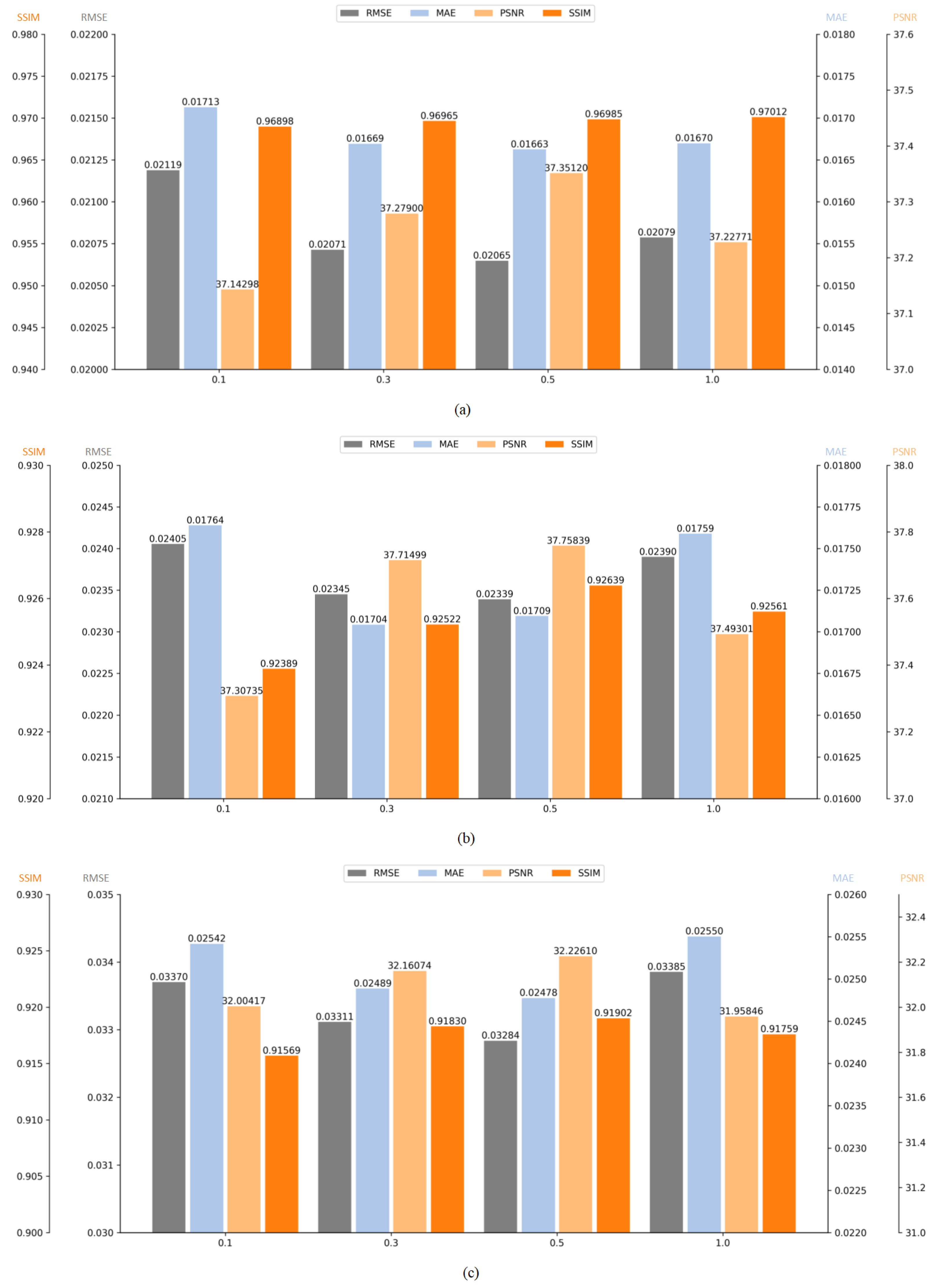
4.5.1. Numerical Evaluations

The results in

Table 4. Quantitative results of different modules in SFCRFormer, where ↑ indicates higher scores are better, ↓ indicates lower scores are preferred and bold indicates the best results.

Dataset	Module					PSNR (↑)	SSIM (↑)	MAE (↓)	RMSE (↓)
	Baseline	DBSA	FreSA	Std. Att.	DDFFN
RICE1	✓	×	×	×	×	36.5432	0.9605	0.01786	0.02273
	✓	✓	×	×	×	36.8385	0.9674	0.01752	0.02174
	✓	×	✓	×	×	36.9646	0.9682	0.01737	0.02128
	✓	✓	✓	×	×	36.9834	0.9685	0.01723	0.02131
	✓	✓	×	✓	✓	36.8753	0.9689	0.01701	0.02095
	✓	✓	✓	×	✓	37.3512	0.9699	0.01662	0.02064
RICE2	✓	×	×	×	×	36.2070	0.9155	0.01884	0.02554
	✓	✓	×	×	×	36.7490	0.9216	0.01894	0.02541
	✓	×	✓	×	×	36.8821	0.9238	0.01773	0.02445
	✓	✓	✓	×	×	37.2963	0.9242	0.01766	0.02419
	✓	✓	×	✓	✓	37.2762	0.9223	0.01767	0.02381
	✓	✓	✓	×	✓	37.7584	0.9264	0.01709	0.02339
T-Cloud	✓	×	×	×	×	30.9301	0.9026	0.02929	0.03837
	✓	✓	×	×	×	31.6029	0.9126	0.02687	0.03521
	✓	×	✓	×	×	31.9512	0.9140	0.02598	0.03473
	✓	✓	✓	×	×	31.9875	0.9152	0.02542	0.03432
	✓	✓	×	✓	✓	32.0129	0.9154	0.02570	0.03391
	✓	✓	✓	×	✓	32.2261	0.9190	0.02477	0.03283

✓ indicates the module is included and × indicates the module is excluded.

demonstrate the importance of each proposed module in SFCRFormer. From the first three rows, it is evident that the removal of either the DBSA or FreSA modules results in a noticeable degradation in model performance. Specifically, the performance drop is more pronounced when the FreSA module is omitted, compared to the DBSA module. To further validate the effectiveness of frequency processing, we replaced the FreSA module with standard attention mechanisms (Std.Att.). As evidenced by the results presented in the last two rows, this substitution led to a significant performance degradation. This indicates that the FFT operation is the fundamental reason for its effectiveness, rather than simply employing attention mechanisms. This underscores the critical role of frequency information in cloud removal tasks and highlights the superiority of the FreSA module in capturing and processing frequency features.

Furthermore, the results of the fourth and last rows in the Table 4 show that the incorporation of the DDFFN module significantly improves the model’s ability to integrate spatial and frequency information. By leveraging the dual-domain fusion capability, the proposed SFCRFormer achieves optimal results across all evaluation metrics, consistently outperforming the baseline and other configurations. This demonstrates the effectiveness of the DDFFN module in enhancing feature representations and improving quantitative performance metrics.

4.5.2. Visualization Analysis

To evaluate the effectiveness of the FreSA module, we generated feature heatmaps before and after processing by the FreSA module, which are shown in Figure 6. As observed in the second column, without the FreSA module’s processing, the contours and edges of objects within the feature map exhibit notable blurriness. However, the results in the third column show that, after processing by FreSA, the edge details of the objects in the feature map are significantly enhanced. These experimental results demonstrate that the FreSA module transforms features from the spatial domain to the frequency domain through FFT and effectively leverages both high- and low-frequency components to improve the model’s ability to capture the details of the objects.

To further evaluate the contributions of the proposed modules in SFCRFormer, we conducted visual results analysis on three datasets: RICE1, RICE2, and T-Cloud. Figure 7, Figure 8 and Figure 9 showcase the qualitative results of the module ablation experiments, where specific regions are enlarged to highlight the cloud removal effectiveness and the restoration of image details.

The results on the thin cloud dataset (Figure 7 and Figure 9) demonstrate that baseline models generate images with blurred edges. In contrast, our proposed method improves the recovery of spatial details, particularly in terms of edge clarity. This comparison highlights the efficacy of our proposed module in addressing cloud removal and fine-grained detail restoration. Furthermore, from Figure 8, which visualizes the thick cloud dataset, it is evident that the baseline model struggles to effectively remove cloud cover, leaving residual cloud artifacts and producing inaccurate patches. When replacing the FreSA module with standard attention mechanisms, the generated cloud-free images exhibit degraded quality and edge blurriness. The proposed SFCRFormer exhibits remarkable performance in eliminating cloud layers and generating high-quality, cloud-free images. By effectively integrating spatial and frequency features, SFCRFormer achieves superior visual results, significantly enhancing image clarity and detail preservation.

4.6. Effects of Different Loss Functions

To systematically evaluate the effectiveness of the loss function, we conduct both ablation studies analyzing the impact of individual loss components on model performance and parameter sensitivity experiments investigating the optimal configurations of key parameters, ensuring the optimal performance of the overall model.

To evaluate the impact of the proposed composite loss function, we conducted an ablation study by training the network using only the $L_c$ loss. The quantitative results, presented in

Table 5. Quantitative results of different loss functions. where ↑ indicates higher scores are better, ↓ indicates lower scores are preferred and bold indicates the best results.

Dataset	Loss		PSNR (↑)	SSIM (↑)	MAE (↓)	RMSE (↓)
	${\mathit{L}}_{\mathit{c}}$	${\mathit{L}}_{\mathit{ssim}}$
RICE1	✓	×	36.8561	0.9673	0.01776	0.02207
	✓	✓	37.3512	0.9699	0.01662	0.02064
RICE2	✓	×	36.2071	0.9155	0.01882	0.02553
	✓	✓	37.7584	0.9264	0.01709	0.02339
T-Cloud	✓	×	30.9301	0.9026	0.02926	0.03835
	✓	✓	32.2261	0.9190	0.02477	0.03283

✓ indicates the module is included and × indicates the module is excluded.

, show that training solely with $L_c$ leads to reduced accuracy across all metrics. This suggests that incorporating SSIM loss significantly enhances the quality of restored images. Specifically, the proposed composite loss function outperforms the $L_c$-only configuration on all datasets, demonstrating the complementary benefits of considering both pixel-level and structural similarities.

Figure 10 provide qualitative comparisons of the ablation experiments for each loss function on the RICE1, RICE2, and T-Cloud datasets, respectively. From these visual results, it is clear that networks trained with only $L_c$ tend to generate artifacts such as patches and striping noise, as shown in the magnified regions. These artifacts do not correspond to the true surface information and severely degrade the visual perception of the restored images. In contrast, the inclusion of SSIM loss significantly reduces these artifacts and stripe noise, resulting in images that are closer to the ground truth in terms of detail and structure.

Additionally, we fine-tuned the weighting parameter $\lambda$ in the loss function to balance the contributions of $L_c$ and $L_{ssim}$. Experiments were conducted on three datasets with $\lambda$ values set to 0.1, 0.3, 0.5, and 1.0. The results, illustrated in Figure 11, indicate that the model achieves optimal performance when $\lambda =0.5$. This configuration effectively balances pixel-level accuracy with structural similarity, maximizing the model’s overall performance. As such, $\lambda$ was set to 0.5 for all experiments.

5. Conclusions

In this paper, we propose a novel cloud removal framework, SFCRFormer, which leverages a cascaded transformer architecture combining spatial and frequency domains to address the challenges of cloud removal in complex scenarios. In the spatial transformer, the DBSA module enhances the extraction of spatial features by simultaneously capturing spatial information and the interrelationships between feature channels through independent branches. In the frequency transformer, the FreSA module introduces frequency information, enabling precise discrimination between cloud-contaminated regions and background areas. The synergistic integration of these modules effectively resolves the confusion between cloud-covered areas and similarly textured ground objects, significantly improving reconstruction accuracy in complex scenes.

Additionally, we introduce the DDFFN, which enhances the extraction of multi-scale cloud and detail features, further improving the network’s ability to restore fine-grained textures. To optimize the model’s performance, we adopt a composite loss function that balances pixel-level accuracy with structural similarity, ensuring both numerical robustness and visual quality in the reconstructed images.

Comprehensive experiments conducted on the RICE and T-Cloud datasets demonstrate the superiority of SFCRFormer. The proposed method achieves state-of-the-art performance, outperforming existing approaches across various quantitative evaluation metrics such as PSNR, SSIM, MAE, and RMSE, while generating visually realistic results that closely approximate the ground truth.

In future work, we plan to extend the application of SFCRFormer to SAR and optical image fusion for cloud removal tasks. By fully exploiting the complementary information provided by these two modalities, we aim to achieve more precise and robust cloud removal results, further broadening the applicability of our framework in diverse remote sensing scenarios.

References

1. Duan, W.; Maskey, S.; Chaffe, P.L.B.; Luo, P.; He, B.; Wu, Y.; Hou, J. Recent Advancement in Remote Sensing Technology for Hydrology Analysis and Water Resources Management. Remote Sens. 2021, 13, 1097. [Google Scholar] [CrossRef]
2. Li, X.; Xu, F.; Tao, F.; Tong, Y.; Gao, H.; Liu, F.; Chen, Z.; Lyu, X. A Cross-Domain Coupling Network for Semantic Segmentation of Remote Sensing Images. IEEE Geosci. Remote Sens. Lett. 2024, 21, 5005105. [Google Scholar] [CrossRef]
3. Himeur, Y.; Rimal, B.; Tiwary, A.; Amira, A. Using artificial intelligence and data fusion for environmental monitoring: A review and future perspectives. Inf. Fusion 2022, 86–87, 44–75. [Google Scholar] [CrossRef]
4. Qing, Y.; Ming, D.; Wen, Q.; Weng, Q.; Xu, L.; Chen, Y.; Zhang, Y.; Zeng, B. Operational earthquake-induced building damage assessment using CNN-based direct remote sensing change detection on superpixel level. Int. J. Appl. Earth Obs. Geoinf. 2022, 112, 102899. [Google Scholar] [CrossRef]
5. Li, Q.; Zhong, R.; Du, X.; Du, Y. TransUNetCD: A Hybrid Transformer Network for Change Detection in Optical Remote-Sensing Images. IEEE Trans. Geosci. Remote Sens. 2022, 60, 5622519. [Google Scholar] [CrossRef]
6. King, M.D.; Platnick, S.; Menzel, W.P.; Ackerman, S.A.; Hubanks, P.A. Spatial and temporal distribution of clouds observed by MODIS onboard the Terra and Aqua satellites. IEEE Trans. Geosci. Remote Sens. 2013, 51, 3826–3852. [Google Scholar] [CrossRef]
7. Xu, F.; Shi, Y.; Yang, W.; Xia, G.S.; Zhu, X.X. CloudSeg: A multi-modal learning framework for robust land cover mapping under cloudy conditions. ISPRS J. Photogramm. Remote Sens. 2024, 214, 21–32. [Google Scholar] [CrossRef]
8. Li, X.; Xu, F.; Liu, F.; Lyu, X.; Tong, Y.; Xu, Z.; Zhou, J. A synergistical attention model for semantic segmentation of remote sensing images. IEEE Trans. Geosci. Remote Sens. 2023, 61, 5400916. [Google Scholar] [CrossRef]
9. Li, X.; Xu, F.; Liu, F.; Tong, Y.; Lyu, X.; Zhou, J. Semantic segmentation of remote sensing images by interactive representation refinement and geometric prior-guided inference. IEEE Trans. Geosci. Remote Sens. 2023, 62, 5400318. [Google Scholar] [CrossRef]
10. Han, S.; Wang, J.; Zhang, S. Former-CR: A transformer-based thick cloud removal method with optical and SAR imagery. Remote Sens. 2023, 15, 1196. [Google Scholar] [CrossRef]
11. Chen, Y.; Cai, Z.; Yuan, J.; Wu, L. A novel dense-attention network for thick cloud removal by reconstructing semantic information. IEEE J. Sel. Top. Appl. Earth Obs. Remote Sens. 2023, 16, 2339–2351. [Google Scholar] [CrossRef]
12. Xia, Q.; Gao, X.; Chu, W.; Sorooshian, S. Estimation of daily cloud-free, snow-covered areas from MODIS based on variational interpolation. Water Resour. Res. 2012, 48, 9523. [Google Scholar] [CrossRef]
13. Zhang, C.; Li, W.; Travis, D.J. Restoration of clouded pixels in multispectral remotely sensed imagery with cokriging. Int. J. Remote Sens. 2009, 30, 2173–2195. [Google Scholar] [CrossRef]
14. Shen, H.; Li, H.; Qian, Y.; Zhang, L.; Yuan, Q. An effective thin cloud removal procedure for visible remote sensing images. ISPRS J. Photogramm. Remote Sens. 2014, 96, 224–235. [Google Scholar] [CrossRef]
15. Yu, G.; Sun, W.B.; Liu, G.; Zhou, M.Y. A Thin Cloud Removal Method for Optical Image Based on Improved Homomorphism Filtering. Appl. Mech. Mater. 2014, 618, 519–522. [Google Scholar] [CrossRef]
16. Li, X.; Jing, Y.; Shen, H.; Zhang, L. The recent developments in cloud removal approaches of MODIS snow cover product. Hydrol. Earth Syst. Sci. 2019, 23, 2401–2416. [Google Scholar] [CrossRef]
17. Hu, G.; Sun, X.; Liang, D.; Sun, Y. Cloud removal of remote sensing image based on multi-output support vector regression. J. Syst. Eng. Electron. 2014, 25, 1082–1088. [Google Scholar] [CrossRef]
18. Tahsin, S.; Medeiros, S.C.; Hooshyar, M.; Singh, A. Optical cloud pixel recovery via machine learning. Remote Sens. 2017, 9, 527. [Google Scholar] [CrossRef]
19. Wang, Q.; Wang, L.; Zhu, X.; Ge, Y.; Tong, X.; Atkinson, P.M. Remote sensing image gap filling based on spatial-spectral random forests. Sci. Remote Sens. 2022, 5, 100048. [Google Scholar] [CrossRef]
20. Li, J.; Zheng, K.; Gao, L.; Ni, L.; Huang, M.; Chanussot, J. Model-Informed Multistage Unsupervised Network for Hyperspectral Image Super-Resolution. IEEE Trans. Geosci. Remote Sens. 2024, 62, 5516117. [Google Scholar] [CrossRef]
21. Li, J.; Zheng, K.; Li, Z.; Gao, L.; Jia, X. X-Shaped Interactive Autoencoders With Cross-Modality Mutual Learning for Unsupervised Hyperspectral Image Super-Resolution. IEEE Trans. Geosci. Remote Sens. 2023, 61, 5518317. [Google Scholar] [CrossRef]
22. Sintarasirikulchai, W.; Kasetkasem, T.; Isshiki, T.; Chanwimaluang, T.; Rakwatin, P. A multi-temporal convolutional autoencoder neural network for cloud removal in remote sensing images. In Proceedings of the 2018 15th International Conference on Electrical Engineering/Electronics, Computer, Telecommunications and Information Technology (ECTI-CON), Chiang Rai, Thailand, 18–21 July 2018; pp. 360–363. [Google Scholar]
23. Goodfellow, I.; Pouget-Abadie, J.; Mirza, M.; Xu, B.; Warde-Farley, D.; Ozair, S.; Courville, A.; Bengio, Y. Generative adversarial networks. Commun. ACM 2020, 63, 139–144. [Google Scholar] [CrossRef]
24. Enomoto, K.; Sakurada, K.; Wang, W.; Fukui, H.; Matsuoka, M.; Nakamura, R.; Kawaguchi, N. Filmy cloud removal on satellite imagery with multispectral conditional generative adversarial nets. In Proceedings of the IEEE Conference on Computer Vision and Pattern Recognition Workshops, Honolulu, HI, USA, 21–26 July 2017; pp. 48–56. [Google Scholar]
25. Wang, Z.; Zhao, J.; Zhang, R.; Li, Z.; Lin, Q.; Wang, X. UATNet: U-shape attention-based transformer net for meteorological satellite cloud recognition. Remote Sens. 2021, 14, 104. [Google Scholar] [CrossRef]
26. Li, W.; Li, Y.; Chen, D.; Chan, J.C.W. Thin cloud removal with residual symmetrical concatenation network. ISPRS J. Photogramm. Remote Sens. 2019, 153, 137–150. [Google Scholar] [CrossRef]
27. Shao, Z.; Pan, Y.; Diao, C.; Cai, J. Cloud detection in remote sensing images based on multiscale features-convolutional neural network. IEEE Trans. Geosci. Remote Sens. 2019, 57, 4062–4076. [Google Scholar] [CrossRef]
28. Li, J.; Zheng, K.; Gao, L.; Han, Z.; Li, Z.; Chanussot, J. Enhanced Deep Image Prior for Unsupervised Hyperspectral Image Super-Resolution. IEEE Trans. Geosci. Remote Sens. 2025, 63, 5504218. [Google Scholar] [CrossRef]
29. Singh, P.; Komodakis, N. Cloud-gan: Cloud removal for sentinel-2 imagery using a cyclic consistent generative adversarial networks. In Proceedings of the IGARSS 2018—2018 IEEE International Geoscience and Remote Sensing Symposium, Valencia, Spain, 22–27 July 2018; pp. 1772–1775. [Google Scholar]
30. Wang, X.; Xu, G.; Wang, Y.; Lin, D.; Li, P.; Lin, X. Thin and thick cloud removal on remote sensing image by conditional generative adversarial network. In Proceedings of the IGARSS 2019—2019 IEEE International Geoscience and Remote Sensing Symposium, Yokohama, Japan, 28 July–2 August 2019; pp. 1426–1429. [Google Scholar]
31. Christopoulos, D.; Ntouskos, V.; Karantzalos, K. Cloudtran: Cloud removal from multitemporal satellite images using axial transformer networks. Int. Arch. Photogramm. Remote Sens. Spat. Inf. Sci. 2022, 43, 1125–1132. [Google Scholar] [CrossRef]
32. Xia, Y.; He, W.; Huang, Q.; Yin, G.; Liu, W.; Zhang, H. CRformer: Multi-modal data fusion to reconstruct cloud-free optical imagery. Int. J. Appl. Earth Obs. Geoinf. 2024, 128, 103793. [Google Scholar] [CrossRef]
33. Jiang, B.; Li, X.; Chong, H.; Wu, Y.; Li, Y.; Jia, J.; Wang, S.; Wang, J.; Chen, X. A deep-learning reconstruction method for remote sensing images with large thick cloud cover. Int. J. Appl. Earth Obs. Geoinf. 2022, 115, 103079. [Google Scholar] [CrossRef]
34. Wu, C.; Xu, F.; Li, X.; Wang, X.; Xu, Z.; Fang, Y.; Lyu, X. Multi-Stage Frequency Attention Network for Progressive Optical Remote Sensing Cloud Removal. Remote Sens. 2024, 16, 2867. [Google Scholar] [CrossRef]
35. He, Q.; Sun, X.; Yan, Z.; Fu, K. DABNet: Deformable contextual and boundary-weighted network for cloud detection in remote sensing images. IEEE Trans. Geosci. Remote Sens. 2021, 60, 5601216. [Google Scholar] [CrossRef]
36. Meraner, A.; Ebel, P.; Zhu, X.X.; Schmitt, M. Cloud removal in Sentinel-2 imagery using a deep residual neural network and SAR-optical data fusion. ISPRS J. Photogramm. Remote Sens. 2020, 166, 333–346. [Google Scholar] [CrossRef] [PubMed]
37. Li, J.; Wu, Z.; Hu, Z.; Zhang, J.; Li, M.; Mo, L.; Molinier, M. Thin cloud removal in optical remote sensing images based on generative adversarial networks and physical model of cloud distortion. ISPRS J. Photogramm. Remote Sens. 2020, 166, 373–389. [Google Scholar] [CrossRef]
38. Ran, X.; Ge, L.; Zhang, X. RGAN: Rethinking generative adversarial networks for cloud removal. Int. J. Intell. Syst. 2021, 36, 6731–6747. [Google Scholar] [CrossRef]
39. Li, X.; Xu, F.; Li, L.; Xu, N.; Liu, F.; Yuan, C.; Chen, Z.; Lyu, X. AAFormer: Attention-Attended Transformer for Semantic Segmentation of Remote Sensing Images. IEEE Geosci. Remote Sens. Lett. 2024, 21, 5002805. [Google Scholar] [CrossRef]
40. Zhang, B.; Zhang, Y.; Li, Y.; Wan, Y.; Yao, Y. CloudViT: A lightweight vision transformer network for remote sensing cloud detection. IEEE Geosci. Remote Sens. Lett. 2022, 20, 5000405. [Google Scholar] [CrossRef]
41. Ge, W.; Yang, X.; Jiang, R.; Shao, W.; Zhang, L. CD-CTFM: A Lightweight CNN-Transformer Network for Remote Sensing Cloud Detection Fusing Multiscale Features. IEEE J. Sel. Top. Appl. Earth Obs. Remote Sens. 2024, 17, 4538–4551. [Google Scholar] [CrossRef]
42. Ma, X.; Huang, Y.; Zhang, X.; Pun, M.O.; Huang, B. Cloud-egan: Rethinking cyclegan from a feature enhancement perspective for cloud removal by combining cnn and transformer. IEEE J. Sel. Top. Appl. Earth Obs. Remote Sens. 2023, 16, 4999–5012. [Google Scholar] [CrossRef]
43. Wang, M.; Song, Y.; Wei, P.; Xian, X.; Shi, Y.; Lin, L. IDF-CR: Iterative Diffusion Process for Divide-and-Conquer Cloud Removal in Remote-sensing Images. IEEE Trans. Geosci. Remote Sens. 2024, 62, 5615014. [Google Scholar] [CrossRef]
44. Chi, K.; Yuan, Y.; Wang, Q. Trinity-Net: Gradient-guided Swin transformer-based remote sensing image dehazing and beyond. IEEE Trans. Geosci. Remote Sens. 2023, 61, 4702914. [Google Scholar] [CrossRef]
45. Li, X.; Xu, F.; Yu, A.; Lyu, X.; Gao, H.; Zhou, J. A Frequency Decoupling Network for Semantic Segmentation of Remote Sensing Images. IEEE Trans. Geosci. Remote Sens. 2025, 63, 5607921. [Google Scholar] [CrossRef]
46. Hsu, W.Y.; Chang, W.C. Wavelet approximation-aware residual network for single image deraining. IEEE Trans. Pattern Anal. Mach. Intell. 2023, 45, 15979–15995. [Google Scholar] [CrossRef] [PubMed]
47. Guo, Y.; He, W.; Xia, Y.; Zhang, H. Blind single-image-based thin cloud removal using a cloud perception integrated fast Fourier convolutional network. ISPRS J. Photogramm. Remote Sens. 2023, 206, 63–86. [Google Scholar] [CrossRef]
48. Zhou, Y.; Feng, Y.; Huo, S.; Li, X. Joint frequency-spatial domain network for remote sensing optical image change detection. IEEE Trans. Geosci. Remote Sens. 2022, 60, 5627114. [Google Scholar] [CrossRef]
49. Jiang, B.; Chong, H.; Tan, Z.; An, H.; Yin, H.; Chen, S.; Yin, Y.; Chen, X. FDT-Net: Deep-Learning Network for Thin-Cloud Removal in Remote Sensing Image Using Frequency Domain Training Strategy. IEEE Geosci. Remote Sens. Lett. 2024, 21, 1002405. [Google Scholar] [CrossRef]
50. Charbonnier, P.; Blanc-Feraud, L.; Aubert, G.; Barlaud, M. Two deterministic half-quadratic regularization algorithms for computed imaging. In Proceedings of the 1st International Conference on Image Processing, Austin, TX, USA, 13–16 November 1994; Volume 2, pp. 168–172. [Google Scholar]
51. Wang, Z.; Bovik, A.C.; Sheikh, H.R.; Simoncelli, E.P. Image quality assessment: From error visibility to structural similarity. IEEE Trans. Image Process. 2004, 13, 600–612. [Google Scholar] [CrossRef]
52. Lin, D.; Xu, G.; Wang, X.; Wang, Y.; Sun, X.; Fu, K. A remote sensing image dataset for cloud removal. arXiv 2019, arXiv:1901.00600. [Google Scholar]
53. Ding, H.; Zi, Y.; Xie, F. Uncertainty-based thin cloud removal network via conditional variational autoencoders. In Proceedings of the Asian Conference on Computer Vision, Macao, China, 4–8 December 2022; pp. 469–485. [Google Scholar]
54. Pan, H. Cloud removal for remote sensing imagery via spatial attention generative adversarial network. arXiv 2020, arXiv:2009.13015. [Google Scholar]
55. Xu, M.; Deng, F.; Jia, S.; Jia, X.; Plaza, A.J. Attention mechanism-based generative adversarial networks for cloud removal in Landsat images. Remote Sens. Environ. 2022, 271, 112902. [Google Scholar] [CrossRef]
56. Zamir, S.W.; Arora, A.; Khan, S.; Hayat, M.; Khan, F.S.; Yang, M.H. Restormer: Efficient transformer for high-resolution image restoration. In Proceedings of the IEEE/CVF Conference on Computer Vision and Pattern Recognition, New Orleans, LA, USA, 18–24 June 2022; pp. 5728–5739. [Google Scholar]
57. Dai, J.; Shi, N.; Zhang, T.; Xu, W. TCME: Thin Cloud removal network for optical remote sensing images based on Multi-dimensional features Enhancement. IEEE Trans. Geosci. Remote Sens. 2024, 62, 5641716. [Google Scholar] [CrossRef]
Figure 1. The overall architecture of the proposed SFCRFormer. (a) The framework of SFCRFormer; (b) Spatial-Frequency Combined Transformer (SFCT).
Remotesensing 17 01499 g001
Figure 2. The structure of our proposed DBSA, FreSA, and DDFFN.
Remotesensing 17 01499 g002
Figure 3. Visualization results of different methods on the RICE1 dataset. (a) Cloudy images; (b) results of the SpA GAN; (c) results of the AMGAN; (d) results of the CVAE; (e) results of the Restormer; (f) results of the TCME; (g) results of ours; (h) ground truth. The enlarged area is indicated by an orange box, and the enlarged result is shown below the original image.
Remotesensing 17 01499 g003
Figure 4. Visualization results of different methods on the RICE2 dataset. (a) Cloudy images; (b) results of the SpA GAN; (c) results of the AMGAN; (d) results of the CVAE; (e) results of the Restormer; (f) results of the TCME; (g) results of ours; (h) ground truth. The enlarged area is indicated by an orange box, and the enlarged result is shown below the original image.
Remotesensing 17 01499 g004
Figure 5. Visualization results of different methods on the T-Cloud dataset. (a) Cloudy images; (b) results of the SpA GAN; (c) results of the AMGAN; (d) results of the CVAE; (e) results of the Restormer; (f) results of the TCME; (g) results of ours; (h) ground truth. The enlarged area is indicated by an orange box, and the enlarged result is shown below the original image.
Remotesensing 17 01499 g005
Figure 6. Heatmaps obtained before and after the FreSA module. (a) Cloudy images; (b) heatmaps obtained before the FreSA module; (c) heatmaps obtained after the FreSA module; (d) ground truth.
Remotesensing 17 01499 g006
Figure 7. Visualization results of module ablation experiment on the RICE1 dataset. (a) Cloudy images; (b) results of the baseline; (c) results of the DBSA; (d) results of the FreSA; (e) results of the DBSA + FreSA; (f) results of the DBSA + Std.Att. + DDFFN; (g) results of ours; (h) ground truth. The enlarged area is indicated by an orange box, and the enlarged result is shown below the original image.
Remotesensing 17 01499 g007
Figure 8. Visualization results of module ablation experiment on the RICE2 dataset. (a) Cloudy images; (b) results of the baseline; (c) results of the DBSA; (d) results of the FreSA; (e) results of the DBSA + FreSA; (f) results of the DBSA + Std.Att. + DDFFN; (g) results of ours; (h) ground truth. The enlarged area is indicated by an orange box, and the enlarged result is shown below the original image.
Remotesensing 17 01499 g008
Figure 9. Visualization results of module ablation experiment on the T-Cloud dataset. (a) Cloudy images; (b) results of the baseline; (c) results of the DBSA; (d) results of the FreSA; (e) results of the DBSA + FreSA; (f) results of the DBSA + Std.Att. + DDFFN; (g) results of ours; (h) ground truth. The enlarged area is indicated by an orange box, and the enlarged result is shown below the original image.
Remotesensing 17 01499 g009
Figure 10. Visualization results of loss function ablation experiment on the different datasets. (a) Cloudy images; (b) results with L c loss; (c) results with the combined loss ( L c + L s s i m ); (d) ground truth. The orange boxes highlight the magnified regions.
Remotesensing 17 01499 g010
Figure 11. Performance of the model under different λ values in the loss function. (a) RICE1 dataset; (b) RICE2 dataset; (c) T-Cloud dataset.
Remotesensing 17 01499 g011