A Near-Real-Time Imaging Algorithm for Focusing Spaceborne SAR Data in Multiple Modes Based on an Embedded GPU

Abstract

To achieve on-board real-time processing for sliding-spotlight mode synthetic aperture radar (SAR), on the one hand, this paper proposes an adaptive and efficient imaging algorithm for the sliding-spotlight mode. On the other hand, a batch processing method was designed and optimized based on the AGX Orin platform to implement the algorithm effectively. Based on the chirp scaling (CS) algorithm, sliding-spotlight mode imaging can be achieved by adding Deramp preprocessing along with either zero-padding or performing an extra chirp scaling operation. This article analyzes the computational complexity of the two algorithms and provides a criterion called the Method Choice Indicator (MCI) for selecting the appropriate method. Additionally, the mathematical expressions for time–frequency transformation are derived, providing the theoretical basis for calculating the equivalent PRF and the azimuth width represented by a single pixel. To increase the size of the data that AGX Orin can process, the batch processing method was proposed to reduce peak memory usage during imaging, so that the limited memory could be better utilized. Meanwhile, this algorithm was also compatible with strip mode and TOPSAR (Terrain Observation by Progressive scans SAR) mode imaging. While batch processing increased data transfers, the integrated architecture of AGX Orin minimized the negative impact. Subsequently, through a series of optimizations of the algorithm, the efficiency of the algorithm was further improved. As a result, it took 19.25 s to complete the imaging process for sliding-spotlight mode data with a size of 42,966 × 27,648. Since satellite data acquisition time was 11.43 s, it can be considered that this method achieved near-real-time imaging. The experimental results demonstrate the feasibility of on-board processing.

1. Introduction

Sliding-spotlight SAR is an imaging mode that lies between the strip-map mode and the spotlight mode [1,2,3,4,5]. It controls the antenna steering direction by constantly focusing on a virtual steering point under the ground. This allows the antenna beam to slide slowly across the imaging area, achieving higher azimuth resolution than in strip mode and a wider azimuth swath than in spotlight mode [6]. However, there are issues of spectral and temporal aliasing in the imaging of sliding-spotlight SAR. The extended CS algorithm can avoid spectral aliasing through sub-aperture processing [7], but this method requires spectrum splicing, which is very complex; moreover, as the azimuth swath increases, the number of sub-apertures also increases, making the subsequent radiometric correction more difficult. The back projection (BP) algorithm directly achieves focusing in the time domain, thereby avoiding the conversion of signals to the Doppler domain [8], which efficiently circumvents the challenge of spectrum aliasing. However, compared to frequency domain algorithms, the BP algorithm incurs a considerable increase in computational load, leading to substantial consumption of computational resources and a marked decrease in processing efficiency.

The CS algorithm for strip mode imaging consists only of FFT and phase multiplication operations, characterized by high imaging accuracy and low computational complexity. Compared to other algorithms such as the range-Doppler (RD) algorithm and the BP algorithm, which require extensive interpolation operations resulting in significantly lower computational efficiency, the CS algorithm has greater potential for real-time processing [9].

Based on the CS algorithm [10], the Deramp preprocessing operation reduces the azimuthal Doppler bandwidth and increases the equivalent PRF, thereby resolving the issue of azimuthal spectral aliasing [11,12,13,14]. By performing azimuth zero-padding after preprocessing or SPECAN post-processing at the end of the algorithm [15], the issue of time-domain aliasing in the imaging results can also be resolved. The main steps of Deramp and SPECAN processing both involve chirp scaling and time–frequency transformation. As a result, this algorithm only requires fast Fourier transform (FFT) and complex multiplication operations, which reduces the computational complexity.

The demand for timeliness in SAR imaging is increasing, and traditional ground-based processing methods can no longer meet these needs. There is an urgent demand for on-board processing to enhance the responsiveness of satellites [16]. However, the current on-board processing capabilities of satellites are primarily focused on the strip mode. As data volumes increase, particularly in the sliding-spotlight SAR mode where the volume of echo data increases significantly, the complexity of imaging processing also rises [17]. Therefore, under the constraint of limited hardware resources, it is of great significance to explore applicable imaging methods to achieve on-board real-time processing for large data volumes in both the strip mode and the sliding-spotlight mode using existing platforms.

The GPU is known for its powerful parallel computing capability and efficient data processing performance, with thousands of small cores designed to handle large volumes of data simultaneously [18,19]. In SAR imaging, these characteristics of GPUs provide significant advantages. Compared to FPGAs [20,21,22,23], GPUs are more suitable for this study. First, the parallel processing capability of a GPU greatly accelerates computationally intensive operations such as range and azimuth compression, speeding up the overall image processing. Additionally, the frequent use of fast Fourier transform (FFT) in SAR imaging is significantly enhanced by optimized GPU libraries like cuFFT [24]. These benefits make GPUs highly effective for real-time SAR imaging and large-scale data processing tasks, enabling the rapid generation of high-resolution SAR images.

Compared to traditional GPUs, embedded GPUs have the advantages of lower power consumption, smaller size, and better integration, making them more suitable for on-board processing. With advancements in technology, embedded GPUs have undergone multiple iterations, continuously improving performance and reducing power consumption. Meanwhile, extensive research has been conducted on different platforms utilizing these GPUs. For example, the implementation of a SAR imaging algorithm on a Jetson TK1 platform is presented in [25]; the implementation and testing of two synthetic aperture radar processing algorithms on a Jetson TX1 platform is described in [26]; in [27], sliding-spotlight SAR imaging based on the NVIDIA Jetson TX2 platform was implemented; and a distributed SAR real-time imaging method based on Jetson Nano platforms is proposed in [23].

This paper focuses on on-board fast imaging for spaceborne sliding-spotlight SAR. Additionally, the algorithm is compatible with both the strip mode and the TOPSAR mode [28,29,30]. The main contributions of this paper are as follows:

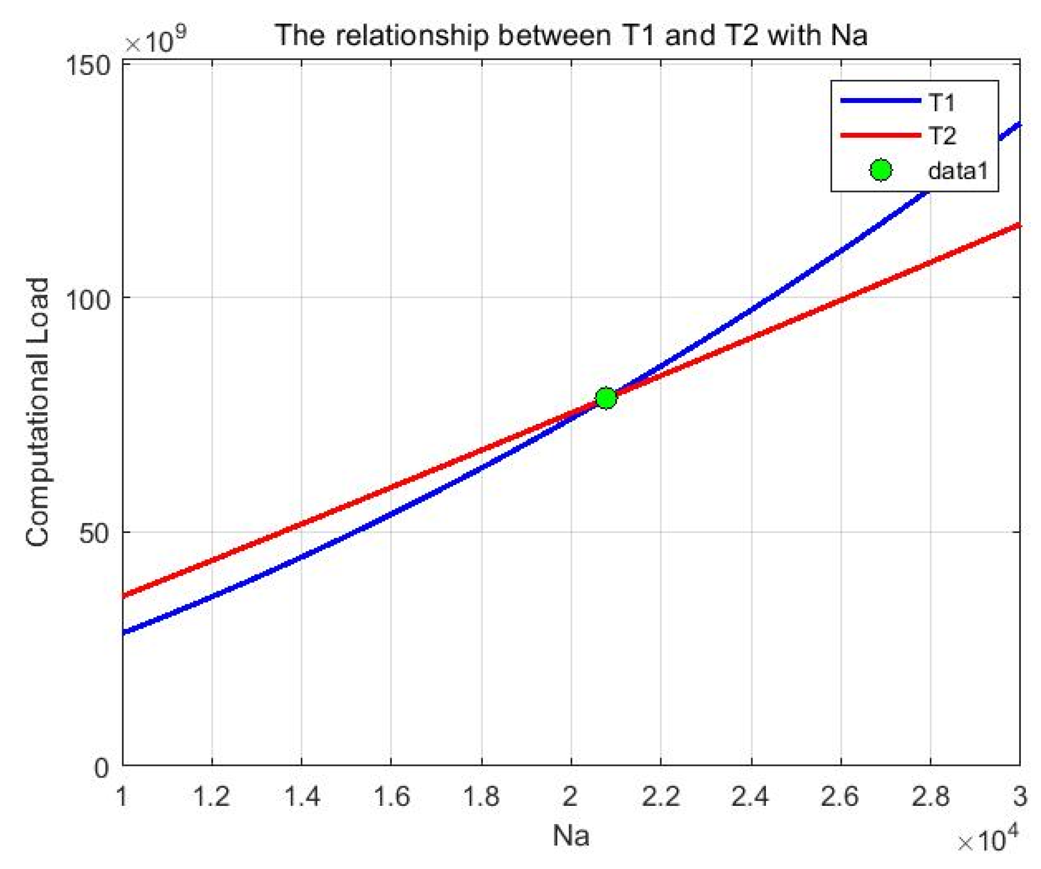
(1) An efficient imaging algorithm based on a criterion called the Method Choice Indicator (MCI) is proposed. Firstly, the theoretical model of the time–frequency transformation is analyzed. Then, the calculation methods of equivalent PRF and azimuth interval of unit pixel are given, which lays a foundation for subsequent geometric correction and calibration. On the other hand, while both azimuth zero-padding and performing a chirp scaling operation once more in post-processing can resolve the issue of time-domain aliasing, the processing time of the two methods will vary with the processed data. The computing efficiency of the two methods is analyzed [9], and the MCI is provided for selecting an efficient method based on specific data.

(2) An application method of this algorithm on the latest generation of the Jetson series, the AGX Orin platform, is proposed, which achieves on-board near-real-time processing for sliding-spotlight mode SAR imaging. To reduce peak memory usage during image processing and enable a single AGX Orin to handle larger datasets, we propose a batch processing method to implement the adaptive and efficient imaging algorithm for the sliding-spotlight mode. Additionally, this algorithm is also compatible with strip mode imaging. Although batch processing increases the number of data transfers between the CPU and GPU, the integrated architecture of the AGX Orin significantly mitigates the negative impact. Furthermore, we have adopted a series of methods to optimize the algorithm, ultimately making it possible to achieve on-board near-real-time processing for large data volumes in the sliding-spotlight mode.

This article is organized as follows: Section 2 analyzes the imaging process of the sliding-spotlight mode. Section 3 presents the algorithm design and optimization methods using the AGX Orin platform. Section 4 gives the experimental results and discussion. Section 5 concludes the paper.

2. Signal Model and Imaging Algorithm

2.1. CS Imaging Algorithm for Strip Mode

The flowchart of the CS algorithm for imaging is shown in Figure 1. The three phase multiplication factors in the figure, $H_1$, $H_2$, and $H_3$, represent the chirp scaling factor, the range migration correction and range compression factor, and the azimuth compensation factor, respectively. The specific calculation methods for these three factors are provided in Section 2.3.

2.2. Azimuth Preprocessing for the Sliding-Spotlight Mode

The imaging geometry model of the spaceborne sliding-spotlight synthetic aperture radar (SAR) is shown in Figure 2. The SAR sensor moves along the $X_I$ axis from $x_{min}^{\prime }$ to $x_{max}^{\prime }$, with the beam center consistently pointing towards the virtual steering point T during this period. $X_f$ represents the azimuth swath width of the scene fully illuminated by the beam. $r_0$ denotes the shortest range between the scene center and the SAR platform, while $r_1$ denotes the shortest range between the scene center and the virtual steering point T. Referring to the imaging geometry, the slant range of the center point in the imaging scene is

$$R\left(\eta \right)=\sqrt{r_0^2+v^2{\eta }^2}$$

(1)

where $v$ is the flight velocity of the SAR sensor, $\eta$ is the azimuth time, and $\eta =0$ indicates the moment when the beam center points to the scene center. Compared with the echo of strip mode, the difference of the echo of the sliding-spotlight mode is mainly the azimuth signal component. The discrete form of the azimuth signal can be written as follows:

$$S_a\left(\eta ,{\eta }_i\right)=\mathrm{r}\mathrm{e}\mathrm{c}\mathrm{t}\left\{{\displaystyle \frac{\eta }{T_s}}\right\}\sum _{i=1}^M\left({\sigma }_i\mathrm{r}\mathrm{e}\mathrm{c}\mathrm{t}\left\{{\displaystyle \frac{\eta -{\eta }_i}{T_p}}\right\}\mathrm{e}\mathrm{x}\mathrm{p}\left(j\pi K_a{\left(\eta -{\eta }_i\right)}^2+j2\pi K_{rot}{\eta }_i\left(\eta -{\eta }_i\right)\right)\right)$$

(2)

where rect{} represents the rectangular function, $T_s$ is the synthetic aperture time of the scene, M is the number of point targets, ${\sigma }_i$ is the scattering coefficient of point targets, ${\eta }_i$ is the azimuth center time, $T_p$ is the synthetic aperture time of the point target, and $K_a$ is the Doppler rate of point targets. $K_{rot}$ is the Doppler rate of the virtual steering point. This paper only considers the case of side-looking, so the Doppler frequency center can be ignored.

To address Doppler ambiguity in the sliding-spotlight mode, azimuth preprocessing is necessary. This preprocessing involves convolving the original signal with a designated reference signal, which is [13]

$$H_{D1}\left(\eta \right)=\mathrm{e}\mathrm{x}\mathrm{p}\left(-j\pi K_{rot}{\eta }^2\right)$$

(3)

This convolution operation can be equivalent to two complex multiplication operations and one FFT operation in the discrete domain. Firstly, the signal is multiplied by the reference function, and we get

$$S_1\left(\eta ,{\eta }_i\right)=\mathrm{r}\mathrm{e}\mathrm{c}\mathrm{t}\left\{{\displaystyle \frac{\eta }{T_s}}\right\}\sum _{i=1}^M\left({\sigma }_i\mathrm{r}\mathrm{e}\mathrm{c}\mathrm{t}\left\{{\displaystyle \frac{\eta -{\eta }_i}{T_p}}\right\}\mathrm{e}\mathrm{x}\mathrm{p}\left(j\pi K_a{\left(\eta -{\eta }_i\right)}^2+j2\pi K_{rot}{\eta }_i\left(\eta -{\eta }_i\right)-j\pi K_{rot}{\eta }^2\right)\right)$$

(4)

At this time, the azimuth bandwidth of the signal has been greatly reduced, and FFT can be performed directly without spectrum aliasing. The result after performing the azimuth FFT is as follows:

$$S_1\left(f,{\eta }_i\right)=\mathrm{r}\mathrm{e}\mathrm{c}\mathrm{t}\left\{{\displaystyle \frac{{\eta }_i+\frac{f}{K_a-K_{rot}}}{T_s}}\right\}\sum _{i=1}^M\left({\sigma }_i\mathrm{r}\mathrm{e}\mathrm{c}\mathrm{t}\left\{{\displaystyle \frac{f}{\left(K_a-K_{rot}\right)T_p}}\right\}\mathrm{e}\mathrm{x}\mathrm{p}\left(j{\phi }_1\left(f\right)\right)\right)$$

(5)

$${\phi }_1\left(f\right)=-{\displaystyle \frac{\pi f^2}{K_a-K_{rot}}}-2\pi {\eta }_{i}f-\pi K_{rot}{\eta }_i^2$$

(6)

where f is the azimuth frequency.

To achieve the time–frequency transformation, let $t=-f/K_{rot}$, then $f=-t{K}_{rot}$, where $t$ is the azimuth time after the time–frequency transformation. Then, $S_1\left(f,{\eta }_i\right)$ is transformed as follows:

$$S_1\left(t,{\eta }_i\right)=\mathrm{r}\mathrm{e}\mathrm{c}\mathrm{t}\left\{{\displaystyle \frac{{\eta }_i-\frac{t{K}_{rot}}{K_a-K_{rot}}}{T_s}}\right\}\sum _{i=1}^M\left({\sigma }_i\mathrm{r}\mathrm{e}\mathrm{c}\mathrm{t}\left\{{\displaystyle \frac{-t{K}_{rot}}{\left(K_a-K_{rot}\right)T_p}}\right\}\mathrm{e}\mathrm{x}\mathrm{p}\left(j{\phi }_1\left(t\right)\right)\right)$$

(7)

$${\phi }_1\left(t\right)=-{\displaystyle \frac{\pi K_{rot}^2{t}^2}{K_a-K_{rot}}}+2\pi {\eta }_i{K}_{rot}t-\pi K_{rot}{\eta }_i^2$$

(8)

Using $f_p$ to represent the original PRF, the duration of the signal after the transformation becomes $f_p/K_{rot}$. Assuming that the number of azimuth sampling points is $N_a$, the time interval of the transformed signal becomes $t_{step}=f_p/K_{rot}/N_a$, and the equivalent PRF after the transformation is $f_{pe}=N_a\cdot K_{rot}/f_p$. After the time–frequency transformation, the equivalent PRF has increased, but the azimuth time support set has decreased. Following another multiplication with $H_{D2}$, which shares the same expression with $H_{D1}$, all azimuth preprocessing steps have been completed. At this point, the signal can be expressed as follows:

$$S_2\left(t,{\eta }_i\right)=\mathrm{r}\mathrm{e}\mathrm{c}\mathrm{t}\left\{{\displaystyle \frac{{\eta }_i-\frac{t{K}_{rot}}{K_a-K_{rot}}}{T_s}}\right\}\sum _{i=1}^M\left({\sigma }_i\mathrm{r}\mathrm{e}\mathrm{c}\mathrm{t}\left\{{\displaystyle \frac{-t{K}_{rot}}{\left(K_a-K_{rot}\right)T_p}}\right\}\mathrm{e}\mathrm{x}\mathrm{p}\left(j{\phi }_2\left(t\right)\right)\right)$$

(9)

$${\phi }_2\left(t\right)=-\pi {\displaystyle \frac{K_a{K}_{rot}}{K_a-K_{rot}}}{t}^2+2\pi {\eta }_i{K}_{rot}t-\pi K_{rot}{\eta }_i^2$$

(10)

It should be noted that although $H_{D2}$ and $H_{D1}$ share the same expression, the number of azimuth sampling points changes after the time–frequency transformation. Therefore, in an actual programming implementation, $H_{D2}$ should be adjusted accordingly.

By Fourier transforming $S_2\left(t,{\eta }_i\right)$, the azimuth spectrum after azimuth preprocessing can be obtained as

$$S_2\left(f,{\eta }_i\right)=\mathrm{r}\mathrm{e}\mathrm{c}\mathrm{t}\left\{{\displaystyle \frac{{\eta }_i-\frac{K_{rot}{\eta }_i-f}{K_a}}{T_s}}\right\}\sum _{i=1}^M\left({\sigma }_i\mathrm{r}\mathrm{e}\mathrm{c}\mathrm{t}\left\{{\displaystyle \frac{{f-K}_{rot}{\eta }_i}{K_a{T}_p}}\right\}\mathrm{e}\mathrm{x}\mathrm{p}\left(j{\phi }_2\left(f\right)\right)\right)$$

(11)

$${\phi }_2\left(f\right)={\displaystyle \frac{\pi f^2}{K_{rot}}}-{\displaystyle \frac{\pi f^2}{K_a}}+{\displaystyle \frac{2\pi {\eta }_i\left(K_{rot}-K_a\right)f}{K_a}}-{\displaystyle \frac{\pi K_{rot}^2{\eta }_i^2}{K_a}}$$

(12)

Azimuth preprocessing involves the convolution of the signal in the time domain with a reference signal, which equates to multiplication with the reference function in the frequency domain. Compared to the azimuth spectrum of the original signal, $S_2\left(f,{\eta }_i\right)$ additionally includes the factor $\pi f^2/K_{rot}$. This confirms the correctness of the time–frequency transformation formula $t=-f/K_{rot}$ and the derivation process. In subsequent imaging, it is necessary to compensate for this phase factor.

2.3. Adaptive Imaging Algorithm for Sliding-Spotlight Mode Using MCI

Figure 3 is the flowchart of the proposed imaging algorithm for processing spaceborne side-looking sliding-spotlight SAR data, where orange blocks represent the preprocessing stage, green blocks correspond to the CS algorithm, and blue blocks indicate the post-processing phase. After azimuth preprocessing, directly using a traditional CS imaging algorithm will result in temporal aliasing in the imaging results. The reason for this issue is that the azimuth time support set of the signal will be reduced after the time–frequency transformation. There are two methods to address this issue. One method involves zero-padding the signal in the azimuth time domain after azimuth preprocessing, directly expanding the time support set. The other method involves performing an additional post-processing step of chirp scaling after completing all phase compensations of CS imaging and before the azimuth inverse Fourier transform. The post-processing also includes a step of the time–frequency transformation, which enhances the time support set while simultaneously altering the azimuth time interval again.

The most critical aspect of the zero-padding method is determining the amount of zero-padding. Based on the previous analysis, the azimuth time interval after the time–frequency transformation is

$$t_{step}=f_p/K_{rot}/N_a$$

(13)

To ensure that the imaging result does not exhibit temporal aliasing, the requirement for the imaging swath must be met. This means that the number of points after zero-padding $N_M$ should satisfy

$$N_M={\mathrm{G}}_{\mathrm{a}\mathrm{z}}/v/t_{step}$$

(14)

where ${\mathrm{G}}_{\mathrm{a}\mathrm{z}}$ is the azimuth swath width, and the zero-padding multiplier is

$$m=N_M/N_a$$

(15)

After zero-padding, the data is processed using the CS algorithm for imaging, which is nearly identical to the imaging process in strip mode, except that $H_3$ requires additional compensation for the phase introduced during preprocessing. The calculations for each factor are as follows [31]:

$$H_1\left(\tau ,f\right)=\exp \left\{-j\pi b_r\left(f;r_{ref}\right)C_s\left(f\right){\left[\tau -{\tau }_{ref}\left(f\right)\right]}^2\right\}$$

(16)

where

$$C_s\left(f\right)={\displaystyle \frac{\sin {\phi }_{ref}}{\sqrt{1-{\left(\frac{\lambda f}{2v}\right)}^2}}}-1$$

(17)

$${\tau }_{ref}\left(f\right)={\displaystyle \frac{2}{c}}{r}_{ref}\left[1+C_s\left(f\right)\right]$$

(18)

$$b_r\left(f;r_{ref}\right)={\displaystyle \frac{K_r}{1+K_r{r}_{ref}\sin {\phi }_{ref}\frac{2\lambda }{c^2}\frac{{\left(\frac{\lambda f}{2v}\right)}^2}{{\left[1-{\left(\frac{\lambda f}{2v}\right)}^2\right]}^{\frac{3}{2}}}}}$$

(19)

$\tau$ is the range time, $r_{ref}$ is the reference range at the midpoint of the synthetic aperture, ${\phi }_{ref}$ is the equivalent squint angle at the reference range, $K_r$ is the frequency modulated (FM) rate of the transmitted signal.

$$H_2\left(f_{\tau },f\right)=\exp \left\{-j{\displaystyle \frac{\pi f_{\tau }^2}{b_r\left(f;r_{ref}\right)\left[1+C_s\left(f\right)\right]}}\right\}\exp \left\{j{\displaystyle \frac{4\pi }{c}}{f}_{\tau }{r}_{ref}{C}_s\left(f\right)\right\}$$

(20)

where $f_{\tau }$ is the range frequency, $c$ is the speed of light.

$$H_3\left(\tau ,f\right)=\exp \left(-j{\displaystyle \frac{2\pi }{\lambda }}c\tau \left(1-\sin {\phi }_{ref}\sqrt{1-{\displaystyle \frac{\lambda f}{2v}}}\right)+j{\displaystyle \frac{\pi }{K_{rot}}}{f}^2\right)\exp \left(j\left[{\Theta }_1\left(f\right)+{\Theta }_2\left(f;r\right)\right]\right)$$

(21)

where

$${\Theta }_1\left(f\right)={\displaystyle \frac{4\pi }{c^2}}{b}_r\left(f;r_{ref}\right)\left[1+C_s\left(f\right)\right]C_s\left(f\right){\left(r{\displaystyle \frac{\sin \phi }{\sin {\phi }_{ref}}}-r_{ref}\right)}^2$$

(22)

$${\Theta }_2\left(f;r\right)={\displaystyle \frac{2\pi rf}{v}}\cos \phi$$

(23)

$r$ is the slant range corresponding to each target, $\phi$ is the corresponding equivalent squint angle. It should be noted that the factor $H_3$ does not contain the component $j{\displaystyle \frac{\pi }{K_{rot}}}{f}^2$ in strip mode.

The chirp scaling post-processing method involves multiplying the signal by a quadratic phase factor $H_{s1}\left(f\right)$ in the range-Doppler domain after completing all phase compensations in the CS algorithm.

$$H_{s1}\left(f\right)=\mathrm{e}\mathrm{x}\mathrm{p}\left(-{\displaystyle \frac{j\pi f^2}{K_2}}\right)$$

(24)

Subsequently, an azimuth inverse Fourier transform is applied, effectively transitioning the signal into the two-dimensional time domain. In the two-dimensional time domain, the signal is multiplied with another quadratic factor

$$H_{s2}\left(t\right)=\mathrm{e}\mathrm{x}\mathrm{p}\left(-j\pi K_2{t}^2\right)$$

(25)

Finally, the azimuth FFT is performed, and the final focused image is obtained in the range-Doppler domain. The final result obtained in the range-Doppler domain is

$$S_3\left(f,{\eta }_i\right)=\sum _{i=1}^M\left(C_1\mathrm{s}\mathrm{i}\mathrm{n}\mathrm{c}\left(\pi T_p{\displaystyle \frac{K_a}{K_2}}\left(f+{\displaystyle \frac{K_2\left(K_{rot}-K_a\right)}{K_a}}{\eta }_i\right)\right)\mathrm{e}\mathrm{x}\mathrm{p}\left(j2\pi C_2{\eta }_{i}f\right)\right)$$

(26)

where $C_1$ and $C_2$ are constants. In the process of achieving the imaging outcome in the range-Doppler domain, a subsequent time–frequency transformation is effectively performed. Let

$$t^{\prime }=-{\displaystyle \frac{f}{K_2}},\mathrm{t}\mathrm{h}\mathrm{e}\mathrm{n} f=-t^{\prime }{K}_2$$

(27)

The new time interval can be calculated by

$$t_{step}^{\prime }={\displaystyle \frac{f_{pe}}{K_2{N}_a}}$$

(28)

Given that

$$f_{pe}=N_a{\displaystyle \frac{K_{rot}}{f_p}}$$

(29)

Then,

$$t_{step}^{\prime }={\displaystyle \frac{K_{rot}}{K_2{f}_p}}$$

(30)

To ensure that the result meets the requirement for azimuth swath width, we have

$$v{t}_{step}^{\prime }{N}_a=G_{az}$$

(31)

Then we can get

$$K_2={\displaystyle \frac{N_a{K}_{rot}v}{f_p{G}_{az}}}$$

(32)

Clearly, when the zero-padding multiplier m is relatively low, using the zero-padding method is more efficient. However, as m increases, the efficiency of the chirp scaling post-processing method gradually exceeds that of the zero-padding method. To determine which method is more efficient for given data, it is necessary to analyze the computational loads of both algorithms. For the zero-padding method, the size of the signal matrix after preprocessing is $m{N}_a\times N_r$, and the computational load primarily involves two azimuth FFTs, two range FFTs, and three complex multiplications of the signal matrix. The total computational load $T_1$ can be calculated by

$$T_1=6\times 3m{N}_a{N}_r+5m{N}_a{N}_r\left(2{\mathit{log}}_2{mN}_a+2{\mathit{log}}_2{N}_r\right)$$

(33)

For the chirp scaling post-processing method, the size of the signal matrix after preprocessing is $N_a\times N_r$, and the computational load primarily involves three azimuth FFTs, two range FFTs, and five complex multiplications of the signal matrix. The total computational load $T_2$ can be calculated by [10]

$$T_2=6\times 5N_a{N}_r+5N_a{N}_r(3{\mathit{log}}_2{N}_a+2{\mathit{log}}_2{N}_r)$$

(34)

Let

$$T\left(m\right)=T_1-T_2$$

(35)

When $T\left(m\right)<0$, the zero-padding method is more efficient; when $T\left(m\right)>0$, the chirp scaling post-processing method is more efficient. It follows that T(m) can be used to select the most efficient method based on specific data. T(m) can be defined as the Method Choice Indicator (MCI).

To provide a more intuitive comparison of the computational loads between the two algorithms under varying data sizes, Figure 4 illustrates the variations of $T_1$ and $T_2$ with $N_a$ under simplified conditions. Since this study focuses on azimuth processing, $N_r$ can be fixed at 10,000, and the relationship between the zero-padding multiple $m$ and $N_a$ is simplified by assuming a linear correlation. Specifically, as $N_a$ increases from 10,000 to 30,000, $m$ linearly rises from 1 to 1.5. Figure 4 reflects, to some extent, the distinct applicable scenarios of the two algorithms.

3. Implementation and Optimization

In this section, the previously discussed CS imaging algorithm for the strip mode and the two imaging algorithms for the sliding-spotlight mode are implemented in a batch-processing manner and optimized on the embedded GPU platform AGX Orin. Given the similar time–frequency characteristics of echo signals in both TOPSAR and sliding-spotlight modes, the proposed algorithm is also well-suited for TOPSAR mode imaging [27,28,29]. The specific content includes the characteristics and advantages of the AGX Orin platform, the method for implementing batch processing, as well as the program optimization method.

3.1. NVIDIA Jetson AGX Orin

The NVIDIA Jetson AGX Orin is classified as a system-on-module (SoM), which primarily belongs to an integrated architecture. In discrete architectures, the CPU and GPU are independent, with the GPU having its own dedicated memory. In contrast, in integrated architectures, the CPU and GPU share the same memory, which greatly speeds up data transfer between the CPU and GPU during batch processing. Furthermore, it uses a GPU based on the Ampere architecture with up to 2048 CUDA cores and 64 Tensor cores, and its CPU is an ARM Cortex-A78AE with 12 cores (Infineon, Neubiberg, Germany), which is designed by ARM Holdings, a semiconductor and software design company headquartered in Cambridge, United Kingdom. The integration of all these components makes it highly efficient. With 64 GB of LPDDR5 memory and a bandwidth of 204.8 GB/s, it is capable of processing much larger scale data. Figure 5a is the image of the AGX Orin, and Figure 5b is the schematic diagram of the integrated architecture.

Although the host and device share the same memory on the AGX Orin platform, explicit data transfers are still typically used for processing, primarily for the following reasons. First, memory access efficiency differs between the GPU and CPU, with GPUs performing better when accessing local cache or dedicated memory regions. Second, memory consistency must be maintained when both access the same data simultaneously, with explicit transfers clearly defining data ownership boundaries and synchronization points. Additionally, despite hardware unified access support, the CUDA programming model traditionally relies on explicit data transfers, influencing existing algorithms and libraries. Finally, GPUs and CPUs have different cache hierarchies, where explicit data movement ensures that data resides at the optimal cache level. While data transfers between the host and device are still necessary, sharing the same memory eliminates the need for data transmission over the PCIe bus, greatly improving transfer efficiency.

When mounting a device on a satellite, factors such as the device’s size, weight, and power consumption must all be carefully considered. The AGX Orin is compact, measuring 105 mm × 105 mm × 50 mm, and weighs approximately 700 g, with maximum power consumption of no more than 60 W, making on-board real-time processing feasible.

3.2. Batch Processing

Although the AGX Orin has 64 GB of memory, many steps in the imaging process, such as calling the cuFFT library for FFT and performing matrix transpositions, require additional memory equivalent to the data size. Therefore, if the entire data block is processed at once, peak memory usage during imaging can be substantial, limiting the size of the data that can be processed. Therefore, it is necessary to perform batch processing on the data.

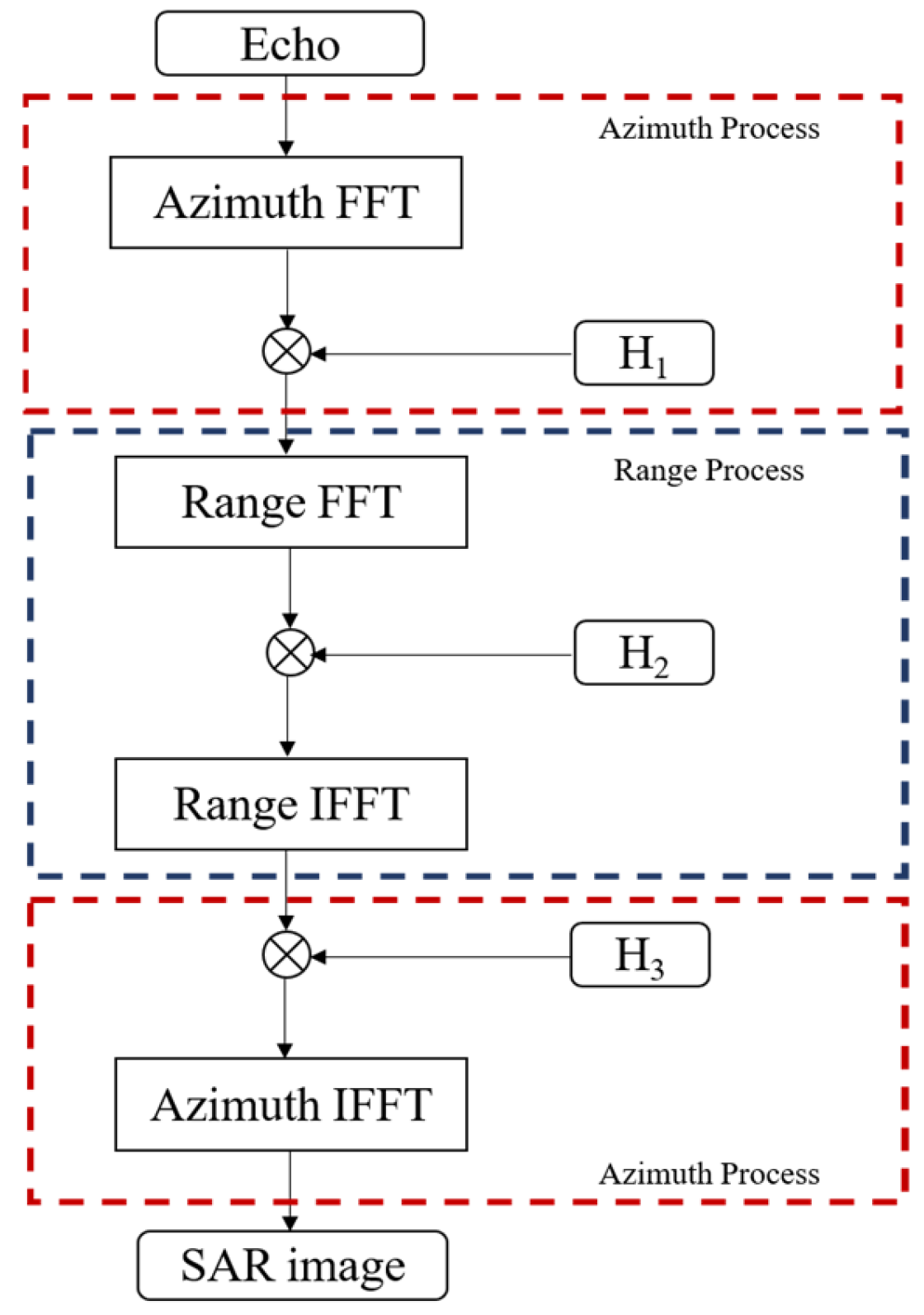
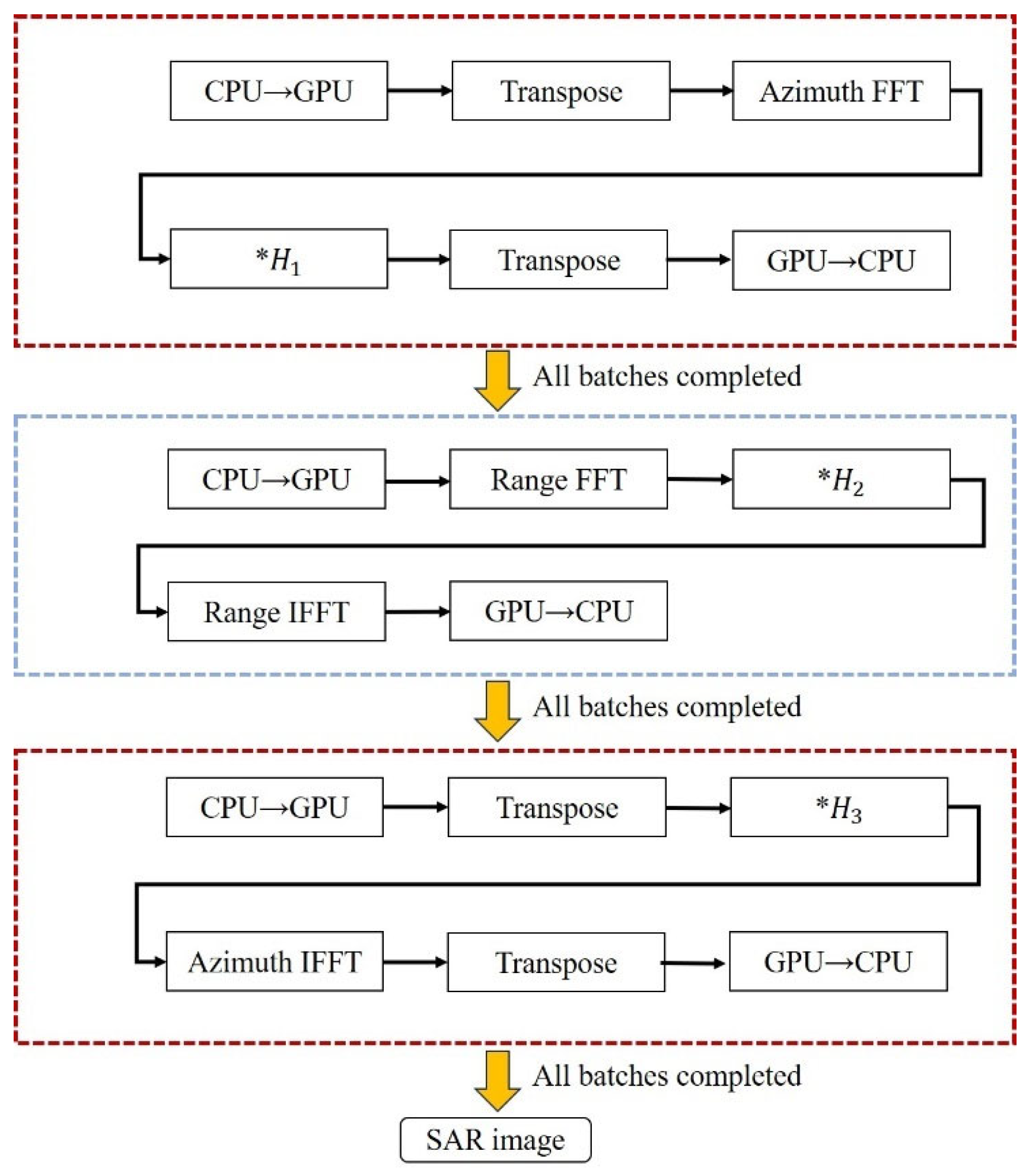
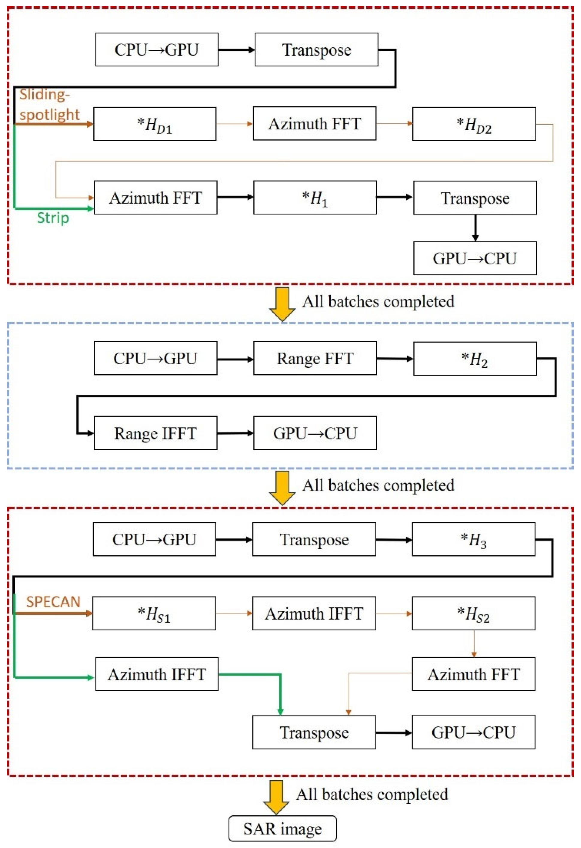
As shown in Figure 1, the CS algorithm for the strip mode can be divided into three parts: the first and third parts handle azimuth processing, while the second part handles range processing. Before processing each part, the data is transferred in batches from the host to the device, and after each batch is processed, the data is transferred back from the device to the host. The complete flowchart of the CS algorithm implementation is shown in Figure 6.

Before the imaging process, the SAR raw data to be processed is read from the file into the host memory $H_0$. As shown on the left side of Figure 7, $H_0$ is arranged in memory in a row-continuous manner, with the range direction being ordered first.

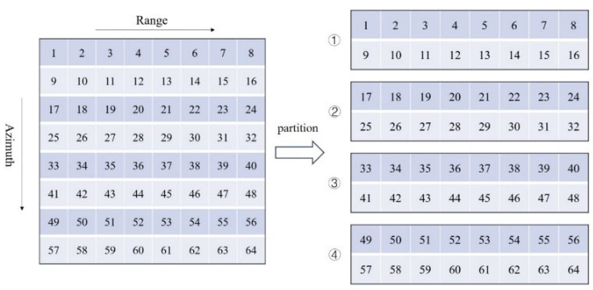
For range processing, the data in the host is partitioned as shown in Figure 7. Each block of data is sequentially copied from the host memory to the device memory. After the range processing is completed, the processed block is copied back to the corresponding position in $H_0$. Since the processed data is continuously arranged, issues related to uncoalesced memory access will not occur.

For azimuth processing, the data in the host is partitioned as shown in Figure 8. Each block of data is still copied from the host memory to the device memory. However, when performing azimuth processing with the current data arrangement, the azimuth data is not contiguous, leading to uncoalesced memory access, which reduces processing efficiency. Therefore, after completing the data transfer from the host to the device, the data needs to be transposed to ensure that during subsequent azimuth processing, coalesced memory access can be achieved to improve efficiency. The arrangement of the transposed data is shown in Figure 8. After completing azimuth processing, the data needs to be transposed again before being copied back to the host, ensuring it can be placed in the correct corresponding position in $H_0$.

By using batch processing, peak memory usage during data transfer is reduced. For example, if the data size in Figure 7 is 8 GB and is divided into four batches for processing, each batch will handle 2 GB of data. Compared to directly transferring the entire data block, which would require 16 GB of memory, batch processing reduces the memory usage to 10 GB.

Batch processing must ensure that the program does not run out of memory during execution, but as the number of chunks increases, the efficiency of the program decreases. Therefore, ideally, fewer chunks are better as long as the program does not overflow the memory. Let $M_{limit}$ denote the available memory of the processor and $S_{data}$ represent the data size. Considering that operations like FFT require additional memory during processing, a safety margin should be reserved. The number of blocks N can be calculated as follows:

$$N=⌈S_{data}/M_{limit}/2⌉$$

(36)

In this formula, dividing by 2 and applying ceiling rounding ensures that the number of blocks is sufficient to avoid memory overflow.

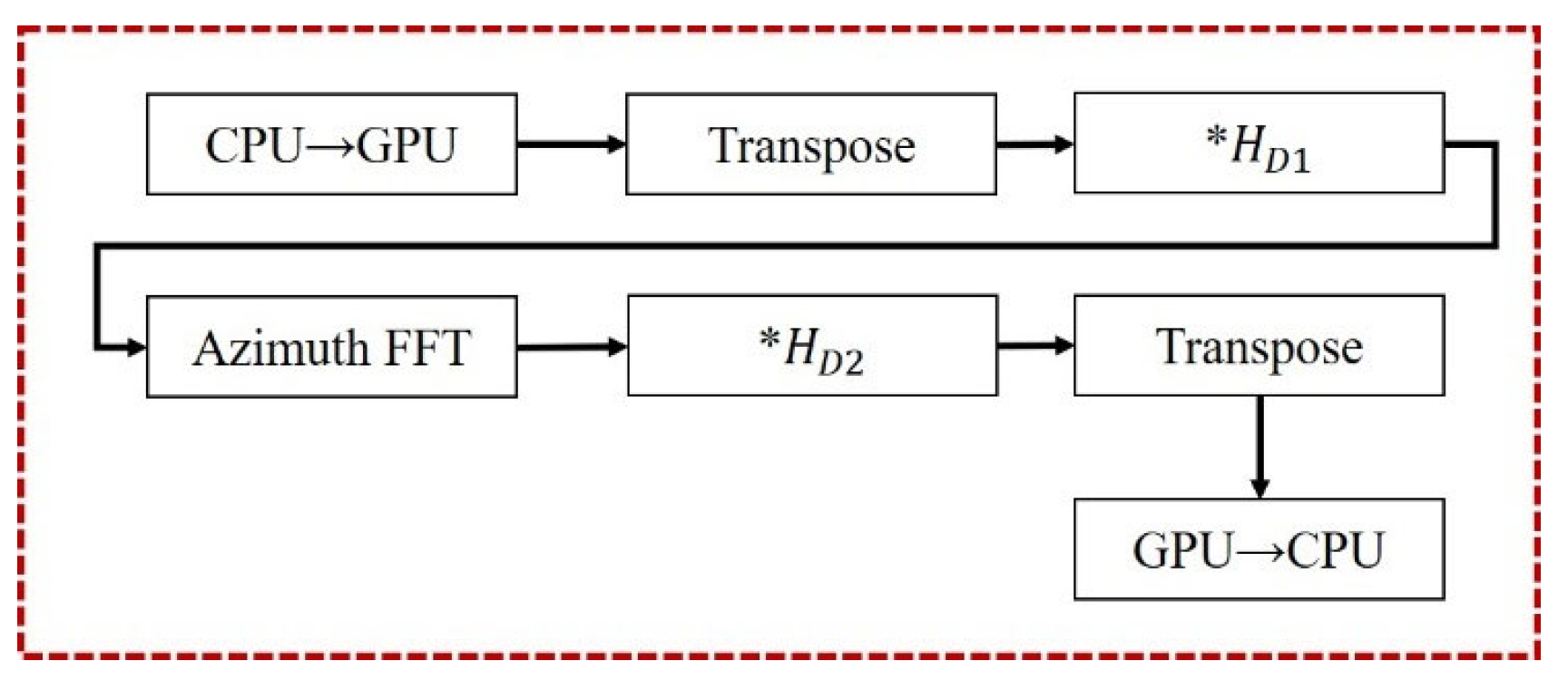
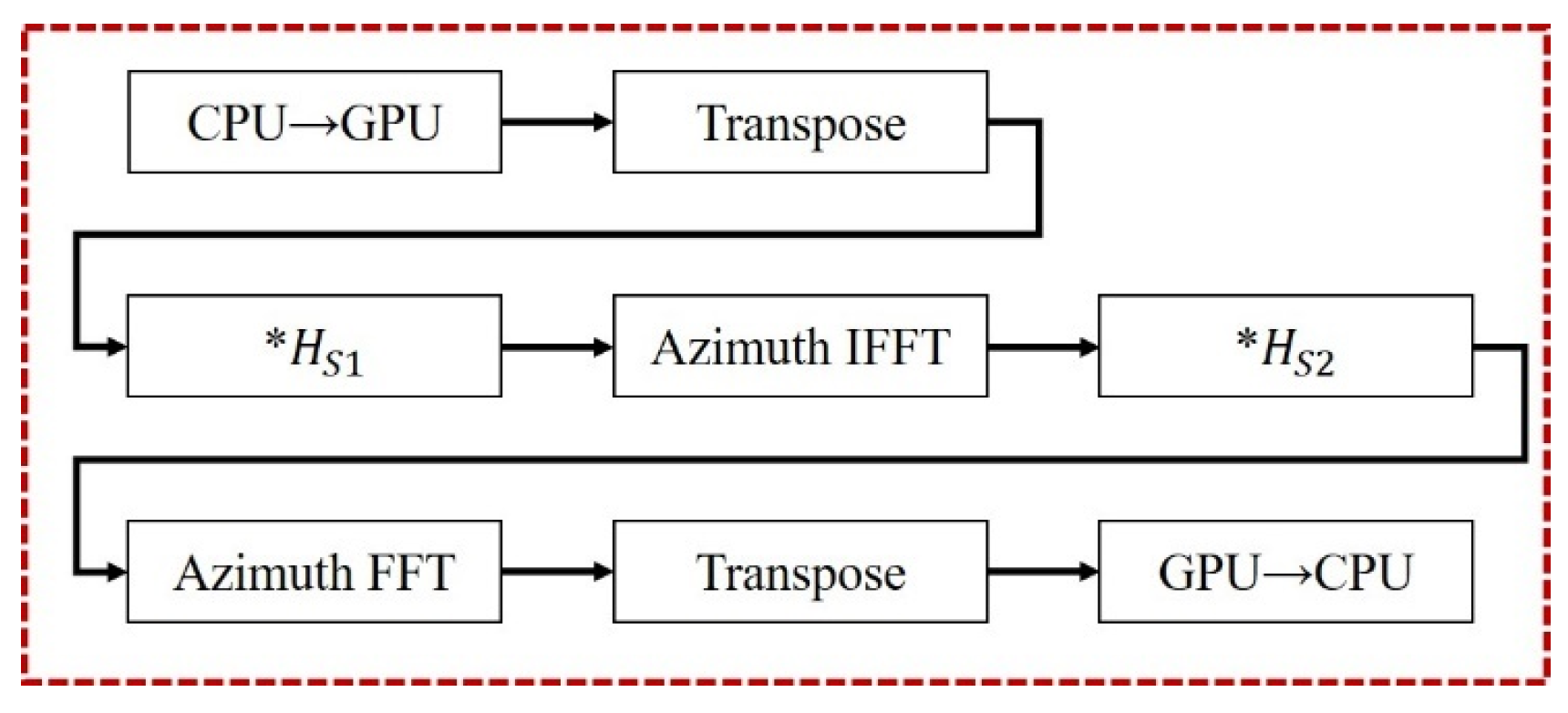
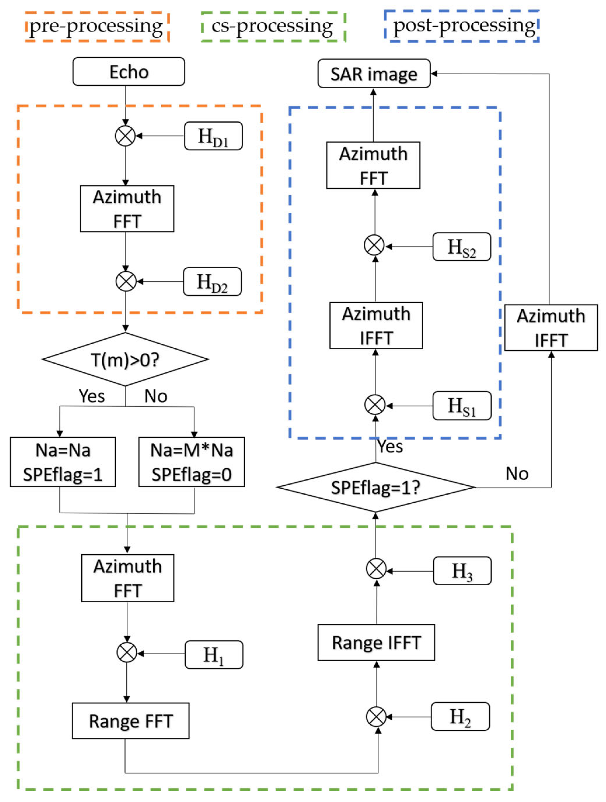
Compared to the CS algorithm in the strip mode, the two imaging algorithms for the sliding-spotlight mode introduce different enhancements: one algorithm adds azimuthal preprocessing, while the other incorporates both preprocessing and post-processing operations. The preprocessing and post-processing steps that need to be added are shown in Figure 9 and Figure 10. As shown in the flowchart in Figure 3, the algorithm can be divided into three parts based on the functions of its individual modules. Since both preprocessing and post-processing are azimuth operations, the entire algorithm, in its most complex form, includes up to four azimuth processing steps and one range processing step. However, this implementation is not optimal.

It can be observed that in the CS algorithm, azimuth processing is involved both immediately after preprocessing and just before post-processing. This means that the two newly added processing steps can be merged into the adjacent azimuth processing steps of the CS algorithm, thereby reducing a total of four data transfers between the host and device as well as four matrix transposition operations.

The complete flowchart of the extended algorithm is shown in Figure 11. Conditional statements can be used to select either the CS imaging algorithm for the strip mode or one of the two algorithms for the sliding-spotlight mode. This algorithm not only enables SAR imaging for both the strip mode and the sliding-spotlight mode but also allows for the selection of a more efficient imaging algorithm based on the characteristics of sliding-spotlight mode data.

3.3. CUDA Programming Techniques and Optimization

Although the algorithm is designed to run on the embedded GPU platform AGX Orin, the methods for writing and optimizing it are almost identical to those used on a traditional GPU and are also implemented using CUDA. From the flowchart of the algorithm, the main steps include data transfer between the CPU and GPU, matrix transposition, FFT and IFFT operations, and phase multiplication. This subsection focuses on how to optimize these parts to improve processing efficiency.

For data transfer between the CPU and GPU during azimuth processing, since the data in a block is not contiguous in memory, block copying can be achieved by calling the memory copy functions cudaMemcpy2D or cudaMemcpy2DAsync provided by the CUDA programming interface, which support segmented copying. For range processing, since the data within a block is stored contiguously, in addition to using the two functions mentioned above, it is also feasible to directly use cudaMemcpy or cudaMemcpyAsync for data transfer. Compared to discrete architectures, the integrated architecture of the AGX Orin platform significantly improves data transfer efficiency between the CPU and GPU. Since multiple data transfers between the CPU and GPU in the program are related to $H_0$, we can register $H_0$ as pinned memory, also known as page-locked memory, to further improve data transfer efficiency. Pinned memory is allocated by locking physical memory pages, which avoids paging operations during data transfers between the CPU and GPU, thereby significantly improving data transfer speed. However, it is important to note that pinned memory consumes more physical memory resources, so it should be used carefully.

The program contains a total of four matrix transposition operations, so the optimization of the matrix transposition is also important. A typical matrix transposition operation involves reading data from global memory by row and writing by column, or reading by column and writing by row, to achieve the transposition effect. However, in such operations, one memory access will inevitably be non-contiguous, resulting in uncoalesced memory access, which ultimately reduces processing efficiency. To address this issue, shared memory can be used to optimize matrix transposition. As shown in Figure 12, the data is read from global memory by row into shared memory. Then, the data is read from shared memory by column and finally written back into global memory by row, completing the matrix transposition. Although the reading from the shared memory is performed column-wise, the access speed within the local memory is very fast, which significantly improves overall performance. The shared memory is divided into banks, and accessing multiple elements from the same bank simultaneously can cause serialization (bank conflicts), leading to performance loss. To avoid this, the data structure is adjusted to ensure that threads access different memory banks. For example, padding arrays can help prevent conflicts.

FFT and IFFT operations can be efficiently implemented using the cuFFT library provided by CUDA. To improve efficiency, the cuFFT plan should be configured once at the beginning of each module and released at the end, rather than configuring and releasing it multiple times.

For the multiple phase multiplication operations in the program, the following optimization techniques can be applied. First, precompute parameters that are used repeatedly in the calculations to avoid repeated computations. In CUDA programming, the pow function is inefficient. For calculating square and cubic terms in the program, replacing the pow function with multiple multiplications can improve efficiency. For instance, use $x \ast x$ for squares and $x \ast x \ast x$ for cubic terms. In addition, the SAR raw data is in single precision, but many parameters used in imaging are in double precision. The program will automatically compute in double precision, which reduces processing efficiency. To improve efficiency, the parameters can be converted from double precision to single precision before imaging, and trigonometric functions like sin and cos can be replaced with their single precision counterparts, sinf and cosf. It is important to note that such changes may lead to a decline in imaging quality. Experiments have shown that while converting other computations to single precision results in outcomes very close to the original and significantly improves efficiency, changing the multiplication with $H_3$ to single precision causes a noticeable degradation in imaging quality.

4. Results

To verify the effectiveness of the methods proposed in this paper, this section will present the experimental results and analysis from Section 2 and Section 3, including both simulation experiments and real-data SAR experiments, as well as the measured results on the AGX Orin platform. The AGX Orin platform was configured with NVIDIA JetPack SDK 5.1.2, including CUDA 11.4.

4.1. Results of Simulated Data

The simulation parameters are listed in

Table 1. List of simulation parameters.

Parameters	Value
Wavelength	$0.03 \mathrm{m}$
Antenna length	$4 \mathrm{m}$
Center line distance	$600 \mathrm{k}\mathrm{m}$
Pulse duration	$20 \mathsf{\mu }\mathrm{s}$
Azimuth width	$27 \mathrm{k}\mathrm{m}$
Pulse bandwidth	$300 \mathrm{M}\mathrm{H}\mathrm{z}$
PRF	$5000 \mathrm{H}\mathrm{z}$
Velocity	$7000 \mathrm{m}/\mathrm{s}$
Squint angle begin	$2°$
Squint angle end	$-2°$
Range width	1 km
Sample frequency	360 MHz

, and a $3\times 3$ dot-matrix is simulated. Figure 13 shows the impulse response functions (IRFs) using the zero-padding method and the post-processing method. Although the IRFs from the zero-padding method appear to have broadened, this was due to the increased density of points after zero-padding. The actual focusing effect was not compromised, as evidenced by the results in

Table 2. Image quality measurement results in the azimuth.

		Range			Azimuth
Methods	Point Target	Resolution (m)	PSLR (dB)	ISLR (dB)	Resolution (m)	PSLR (dB)	ISLR (dB)
Zero-padding method	a	0.44	−13.27	−10.08	0.90	−13.54	−12.19
	b	0.44	−13.25	−10.03	0.79	−13.25	−11.54
	c	0.44	−13.33	−10.13	0.91	−13.13	−12.21
Post-processing method	a	0.44	−13.28	−10.12	0.91	−13.29	−10.49
	b	0.44	−13.25	−10.03	0.82	−13.26	−10.08
	c	0.44	−13.35	−10.18	0.91	−13.40	−10.78

. The obtained quality measurement parameters, including impulse response width, peak sidelobe ratio (PSLR), and integrated sidelobe ratio (ISLR), in the azimuth were calculated and are listed in Table 2. It can be observed that the three point targets located along the diagonal in the scene were well focused.

4.2. Real Data Results

The parameters of the satellite used for imaging data are shown in

Table 3. Some parameters of the satellite used.

Parameters	Value
Wavelength	$0.0555 \mathrm{m}$
Center line distance	$971.68 \mathrm{k}\mathrm{m}$
Pulse duration	$45 \mathsf{\mu }\mathrm{s}$
Pulse bandwidth	$240 \mathrm{M}\mathrm{H}\mathrm{z}$
PRF	$3759.22 \mathrm{H}\mathrm{z}$
Velocity	$7121.65 \mathrm{m}/\mathrm{s}$
Sample frequency	266.67 MHz

. Figure 14a,b shows the imaging results of a set of data acquired by a SAR satellite, both of which were focused well. Subsequently, multiple sets of real data were imaged, and the processing time was recorded.

Table 4. Time consumption comparison.

	Zero-Padding Method	Proposed Method	Adaptive Method
Data1	37.50 s	51.13 s	37.50 s
Data2	74.27 s	24.86 s	24.86 s
Data3	123.72 s	35.89 s	35.89 s

shows the time taken to complete the imaging process for three different sets of real data under the same conditions. It can be observed that the zero-padding method took less time than the post-processing method did for Data1, and the post-processing method took less time than the zero-padding method did for Data2 and Data3. Since $T\left(m\right)<0$ for Data1 and $T\left(m\right)>0$ for Data2 and Data3, the time taken by the proposed method was consistently the shorter of the two methods. This verifies the effectiveness of the algorithm selection strategy.

4.3. Experiments on the AGX Orin

In this subsection, the CUDA programming techniques and optimization methods presented in the previous section are implemented on the AGX Orin platform. The experimental results were recorded and analyzed throughout the process.

The AGX Orin was set to operate in 60 W mode to ensure it achieved its optimal performance.

Table 5. Time consumption and speedup ratio after optimization.

Order/n	Optimization	Time Consumption$/{\mathit{t}}_{\mathit{n}}$	Speedup Ratio
0	Directly add preprocessing and post-processing based on the CS	67.02 s
1	Optimize the processing workflow according to Figure 10	60.22 s	1.11
2	$H_0$ as pinned memory	55.01 s	1.22
3	Optimize phase multiplication	20.67 s	3.24
4	Optimize matrix transposition	19.25 s	3.48

presents the execution times of the program after each step of optimization, in sequential order, along with the speedup ratio compared to the original, non-optimized version. Assuming the initial time consumption of the program is $t_0$, and after n steps of optimization, the time consumption becomes $t_n$, then the total speedup ratio after optimizations is:

$$S_n={\displaystyle \frac{t_0}{t_n}}$$

(37)

The tests were conducted using the post-processing algorithm in the sliding-spotlight mode, as this algorithm included the most comprehensive set of operations, making it a better reflection of the overall performance improvements of the program. The data size was 42,966 $\times$ 27,648. As shown in Table 5, each optimization method improved efficiency in different degrees. The most significant improvement was seen after optimizing the phase multiplication, since phase multiplication constituted the main body of the algorithm and involved the greatest amount of optimization content.

5. Discussion

The final optimized imaging processing time was 19.25 s, while the satellite acquisition time for the data was 11.43 s. The ratio of data acquisition time to processing time was

$${\displaystyle \frac{t_{\mathrm{a}\mathrm{c}\mathrm{q}\mathrm{u}\mathrm{i}\mathrm{s}\mathrm{i}\mathrm{t}\mathrm{i}\mathrm{o}\mathrm{n}}}{t_{\mathrm{i}\mathrm{m}\mathrm{a}\mathrm{g}\mathrm{i}\mathrm{n}\mathrm{g}}}}={\displaystyle \frac{11.43\mathrm{s}}{19.25\mathrm{s}}}\approx 0.59$$

(38)

Typically, when this ratio reaches 1, the processing can be considered real-time. Therefore, the optimized processing can be regarded as near-real-time processing [32,33].

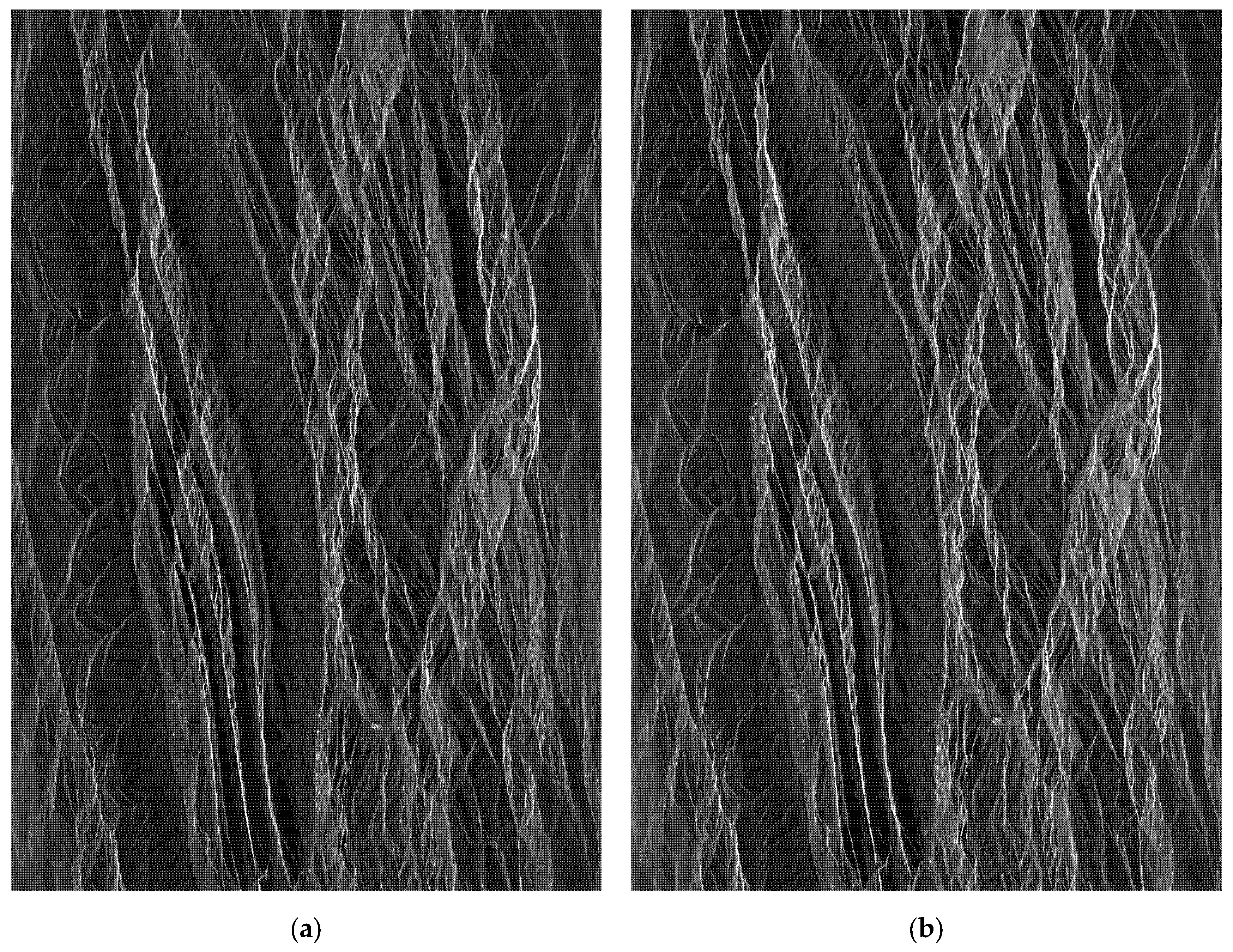
Figure 15 shows the final imaging result after a series of optimizations listed in Table 5. It can be observed that there was no significant difference in image quality compared to that of the original result.

It took 54 s before optimization compared to 20 s after optimization to image the same data using the zero-padding method, resulting in a speedup ratio of 2.7. Using another set of data in the strip mode with a size of 21,211 $\times$ 39,424 for CS algorithm imaging, the processing time was 23.4 s before optimization and 7.7 s after optimization, resulting in a speedup ratio of 3.0.

In addition, the optimized program was ported to NVIDIA A6000 (designed by NVIDIA Corporation, Santa Clara, USA; GPU chips fabricated by TSMC, Hsinchu, Taiwan, China) for experimentation. Using the same data in the sliding-spotlight mode as before, with the post-processing method for imaging, the processing time was approximately 9.5 s. Although the A6000 took less time than the AGX Orin did, it had higher power consumption than the AGX Orin. To better compare the performance of the algorithm on the two platforms, the performance-to-power ratio can be used as a reference. Since the same data was used, the data size can be excluded from the formula, leaving only time and power. Clearly, the product of time and power is a representation of energy, which can be understood as the amount of energy consumed during the imaging process for this data. Since the A6000 has a power consumption of 300 W and the AGX Orin has a power consumption of 60 W, the energy consumed during the imaging process is 2850 J and 1320 J, respectively. Therefore, the AGX Orin demonstrates better overall performance compared to the A6000. A major reason is that the A6000 uses a discrete architecture, which results in lower data transfer efficiency between the CPU and GPU. The A6000 is more suited for ground processing, as it is not constrained by factors such as size, weight, and power consumption.

6. Conclusions

In this article, an adaptive and efficient imaging algorithm was proposed to process spaceborne sliding-spotlight SAR data. A selection criterion called the MCI for the two methods was provided. This is the basis for implementing and optimizing the algorithm on the AGX Orin. Furthermore, a detailed analysis of the changes in the signal before and after the time–frequency transformation and its function in Deramp preprocessing and chirp scaling post-processing were introduced, laying the foundation for subsequent geometric correction and calibration.

Subsequently, the batch processing design and optimization of the algorithm were carried out on the AGX Orin. As a result, imaging in the sliding-spotlight mode for data of size 42,966 $\times$ 27,648 was completed in just 22 s, achieving a speedup ratio of 2.9. This makes near-real-time SAR imaging for large datasets in the sliding-spotlight mode on-board possible. In addition, the proposed algorithm is compatible with both the strip mode and the sliding-spotlight mode imaging algorithms. The algorithm is also applicable to the TOPSAR mode. Finally, a comparison between the AGX Orin and A6000 was conducted, showing that the AGX is more suitable for on-board processing.

References

1. Lanari, R.; Zoffoli, S.; Sansosti, E.; Fornaro, G.; Serafino, F. New approach for hybrid strip-map/spotlight SAR data focusing. IEE Proc.-Radar Sonar Navig. 2001, 148, 363–372. [Google Scholar] [CrossRef]
2. Luo, X.; Deng, Y.; Wang, R.; Xu, W.; Luo, Y.; Guo, L. Image formation processing for sliding spotlight SAR with stepped frequency chirps. IEEE Geosci. Remote Sens. Lett. 2014, 11, 1692–1696. [Google Scholar]
3. Xu, W.; Deng, Y.; Huang, P.; Wang, R. Full-aperture SAR data focusing in the spaceborne squinted sliding-spotlight mode. IEEE Trans. Geosci. Remote Sens. 2014, 52, 4596–4607. [Google Scholar] [CrossRef]
4. Yang, W.; Chen, J.; Liu, W.; Wang, P.; Li, C. A modified three-step algorithm for TOPS and sliding spotlight SAR data processing. IEEE Trans. Geosci. Remote Sens. 2017, 55, 6910–6921. [Google Scholar] [CrossRef]
5. Sun, G.; Wu, Y.; Yang, J.; Xing, M.; Bao, Z. Full-aperture focusing of very high resolution spaceborne-squinted sliding spotlight SAR data. IEEE Trans. Geosci. Remote Sens. 2017, 55, 3309–3321. [Google Scholar] [CrossRef]
6. Belcher, D.P.; Baker, C.J. High resolution processing of hybrid strip-map/spotlight mode SAR. IEE Proc.-Radar Sonar Navig. 1996, 143, 366–374. [Google Scholar] [CrossRef]
7. Mittermayer, J.; Lord, R.; Borner, E. Sliding spotlight SAR processing for TerraSAR-X using a new formulation of the extended chirp scaling algorithm. In Proceedings of the IGARSS 2003, Toulouse, France, 21–25 July 2003; Volume 3, pp. 1462–1464. [Google Scholar]
8. Yin, C.B.; Ran, D. Converse beam cross sliding spotlight SAR imaging processing with data-blocking based fast back projection. In Proceedings of the IGARSS 2016, Beijing, China, 10–15 July 2016; pp. 1070–1073. [Google Scholar]
9. Cumming, I.G.; Wong, F.H. Digital Processing of Synthetic Aperture Radar Data: Algorithms and Implementation; Artech House: Boston, MA, USA, 2005. [Google Scholar]
10. Raney, R.K.; Runge, H.; Bamler, R.; Cumming, I.G.; Wong, F.H. Precision SAR processing using chirp scaling. IEEE Trans. Geosci. Remote Sens. 1994, 32, 786–799. [Google Scholar] [CrossRef]
11. Lanari, R.; Tesauro, M.; Sansosti, E.; Fornaro, G. Spotlight SAR data focusing based on a two-step processing approach. IEEE Trans. Geosci. Remote Sens. 2001, 39, 1993–2004. [Google Scholar] [CrossRef]
12. Prats, P.; Scheiber, R.; Mittermayer, J.; Meta, A.; Moreira, A. Processing of sliding spotlight and TOPS SAR data using baseband azimuth scaling. IEEE Trans. Geosci. Remote Sens. 2010, 48, 770–780. [Google Scholar] [CrossRef]
13. Wang, G.D.; Zhou, Y.Q.; Li, C.S. A Deramp Chirp Scaling algorithm for high-resolution spaceborne spotlight SAR imaging. J. Electron. 2003, 31, 1784–1789. [Google Scholar]
14. Han, X.L.; Li, S.Q.; Wang, Y.; Yu, W.D. Study on squint sliding spotlight mode SAR imaging. J. Electron. Inf. Technol. 2013, 35, 2843–2849. [Google Scholar] [CrossRef]
15. Wang, P.B.; Chen, J.; Li, C.S.; Yang, W. Imaging algorithm for sliding spotlight SAR data based on improved Deramp processing. In Proceedings of the Ninth National Conference on Information Acquisition and Processing I, Harbin, China, 10–12 June 2011. [Google Scholar]
16. Deng, Y.; Yu, W.; Zhang, H.; Wang, W.; Liu, D.; Wang, Y. Development trends of future spaceborne SAR technology. J. Radars 2020, 9, 1–33. [Google Scholar]
17. Cai, M.; Wang, H.; Hua, W. Research on optimal design of spaceborne SAR real-time imaging technology based on FPGA. In Proceedings of the 2nd China International SAR Symposium, Shanghai, China, 3–5 November 2021; pp. 1–2. [Google Scholar]
18. Nickolls, J.; Dally, W. The GPU computing era. IEEE Micro 2010, 30, 56–69. [Google Scholar] [CrossRef]
19. Cui, Z.; Quan, H.; Cao, Z.; Xu, S.; Ding, C.; Wu, J. SAR target CFAR detection via GPU parallel operation. IEEE J. Sel. Top. Appl. Earth Observ. Remote Sens. 2018, 11, 4884–4894. [Google Scholar] [CrossRef]
20. Yu, W.; Xie, Y.; Lu, D.; Li, B.; Chen, H.; Chen, L. Algorithm implementation of on-board SAR imaging on FPGA+DSP platform. In Proceedings of the IEEE International Conference on Signal, Information and Data Processing, Chongqing, China, 11–13 December 2019; pp. 1–5. [Google Scholar]
21. Mota, D.; Cruz, H.; Miranda, P.; Duarte, R.; Sousa, J.; Neto, H. Onboard processing of synthetic aperture radar back-projection algorithm in FPGA. IEEE J. Sel. Top. Appl. Earth Observ. Remote Sens. 2022, 15, 3600–3611. [Google Scholar] [CrossRef]
22. Li, B.; Shi, H.; Chen, L.; Yu, W.; Yang, C.; Xie, Y.; Bian, M.; Zhang, Q.; Pang, L. Real-time spaceborne synthetic aperture radar float-point imaging system using optimized mapping methodology and a multi-node parallel accelerating technique. Sensors 2018, 18, 725. [Google Scholar] [CrossRef]
23. Yang, T.; Xu, Q.; Meng, F.; Zhang, S. Distributed real-time image processing of formation flying SAR based on embedded GPUs. IEEE J. Sel. Top. Appl. Earth Observ. Remote Sens. 2022, 15, 6495–6505. [Google Scholar] [CrossRef]
24. Meng, D.; Hu, Y.; Shi, T.; Sun, R.; Li, X. CUDA design and implementation of real-time imaging processing algorithm for airborne SAR based on NVIDIA GPU. J. Radars 2013, 2, 481–491. [Google Scholar] [CrossRef]
25. Fatica, M.; Phillips, E. Synthetic aperture radar imaging on a CUDA-enabled mobile platform. In Proceedings of the IEEE High Performance Extreme Computing Conference, Waltham, MA, USA, 9–11 September 2014; pp. 1–5. [Google Scholar]
26. Pavlov, V.A.; Belov, A.A.; Tuzova, A.A. Implementation of synthetic aperture radar processing algorithms on the Jetson TX1 platform. In Proceedings of the IEEE International Conference on Electrical Engineering and Photonics, St. Petersburg, Russia, 14–17 October 2019; pp. 90–93. [Google Scholar]
27. Hu, S.; Li, H.; Li, W.; Xie, Y.; Chen, L.; Chen, W. The real-time imaging method for sliding spotlight SAR based on embedded GPU. J. Beijing Polytech. Univ. 2020, 40, 1018–1025. [Google Scholar]
28. Yang, W.; Li, C.; Chen, J.; Wang, P. A novel three-step focusing algorithm for TOPSAR image formation. In Proceedings of the 2010 IEEE International Geoscience and Remote Sensing Symposium, Honolulu, HI, USA, 25–30 July 2010; pp. 4087–4090. [Google Scholar]
29. Chen, Q.; Huang, H.F.; He, F.; Liang, D.N.; Dong, Z. Full Aperture Imagining Algorithm of TOPSAR Based on Frequency Domain Extension and SPECAN. J. Electron. Inf. Technol. 2012, 34, 2445–2450. [Google Scholar] [CrossRef]
30. Xu, W.; Deng, Y.K. Imaging Algorithm of Spaceborne TOPSAR Data Based on Two-dimension Chirp-Z Transform. J. Electron. Inf. Technol. 2011, 33, 2679–2685. [Google Scholar] [CrossRef]
31. Huang, Y.; Li, C.; Chen, J.; Zhou, Y. Refined chirp scaling algorithm for high resolution spaceborne SAR imaging. J. Acta Electron. Sin. 2000, 3, 35–38. [Google Scholar]
32. Tang, X.; Bratley, K.H.; Cho, K.; Bullock, E.L.; Olofsson, P.; Woodcock, C.E. Near real-time monitoring of tropical forest disturbance by fusion of Landsat, Sentinel-2, and Sentinel-1 data. J. Remote Sens. Environ. 2023, 294, 113626. [Google Scholar] [CrossRef]
33. Zhang, P.; Qin, Q.; Zhang, S.; Zhao, X.; Yan, X.; Wang, W.; Zhang, H. Near real-time remote sensing based on satellite internet: Architectures, key techniques, and experimental progress. Aerospace 2024, 11, 167. [Google Scholar] [CrossRef]
Figure 1. Flowchart of the CS imaging algorithm.
Remotesensing 17 01495 g001
Figure 2. Imaging geometry model of the spaceborne sliding-spotlight SAR.
Remotesensing 17 01495 g002
Figure 3. Flowchart of the adaptive imaging algorithm.
Remotesensing 17 01495 g003
Figure 4. The relationship between T 1 and T 2 with N a .
Remotesensing 17 01495 g004
Figure 5. NVIDIA Jetson AGX Orin. (a) Overview image. (b) Diagram of integrated architecture.
Remotesensing 17 01495 g005
Figure 6. Flowchart of the CS algorithm implemented using batch processing.
Remotesensing 17 01495 g006
Figure 7. Schematic diagram of H 0 partitioned along the azimuth direction.
Remotesensing 17 01495 g007
Figure 8. Schematic diagram of H 0 partitioned along the range direction and transposed.
Remotesensing 17 01495 g008
Figure 9. Flowchart of preprocessing.
Remotesensing 17 01495 g009
Figure 10. Flowchart of post-processing.
Remotesensing 17 01495 g010
Figure 11. Flowchart of the algorithm for both strip and sliding-spotlight modes.
Remotesensing 17 01495 g011
Figure 12. Schematic diagram of matrix transposition.
Remotesensing 17 01495 g012
Figure 13. Contour plots of the IRF from the three point targets located along the diagonal using (ac) the zero-padding method and (df) the post-processing method.
Remotesensing 17 01495 g013aRemotesensing 17 01495 g013b
Figure 14. Results from spaceborne SAR data when using (a) the zero-padding method (b) and the post-processing method.
Remotesensing 17 01495 g014
Figure 15. Results after optimization.
Remotesensing 17 01495 g015