TPNet: A High-Performance and Lightweight Detector for Ship Detection in SAR Imagery

Abstract

The advancement of SAR satellites enables continuous and real-time ship monitoring on water surfaces regardless of time and weather. Traditional ship detection algorithms in SAR imagery using manually designed operators lack accuracy, while many existing deep learning-based detection algorithms are computationally intensive and have room for accuracy improvement. Inspired by CenterNet, we propose the Three Points Network (TPNet). It locates the ship’s center point and estimates distances to the top-left and bottom-right corners for precise positioning. We introduce several innovative mechanisms to enhance TPNet’s performance, improving both accuracy and computational efficiency. Evaluated on the open-source SAR-Ship-Dataset, TPNet outperforms 14 other deep learning-based detection algorithms in accuracy and efficiency. Its strong generalization ability is further verified on SSDD and HRSID datasets. These results show TPNet’s potential in real-time maritime surveillance and monitoring systems.

1. Introduction

Synthetic Aperture Radar (SAR) technology, with its active microwave sensor, has emerged as a valuable tool in marine science due to its ability to operate effectively in all weather and lighting conditions. Since the launch of the SEASAT1 satellite by the United States in 1978, SAR technology has been widely utilized, and many countries have launched their own SAR satellites, leading to a surge of interest in the processing of SAR images. In particular, ship detection algorithms for SAR images have emerged as a significant research focus in remote sensing, attracting growing attention from researchers and practitioners dedicated to developing advanced detection techniques. Traditional ship detection algorithms generally employ a sliding window approach to partition an image into smaller regions. Within each region, hand-crafted features such as HOG [1], LBP [2], DoG [3] or SIFT [4] are extracted. Subsequently, a classification algorithm, typically a Support Vector Machine (SVM), is applied to ascertain the presence of a ship within each region. For example, Gan et al. [5] utilized a continuous interval rotating sliding window and HOG features to locate ships. Lin et al. [6] put forward a compact and effective feature named MSHOG, which can be computed by four steps to classify ships in SAR images. Wang et al. [7] proposed a detector based on DoG to detect ships in Radarsat-2 ScanSAR data. Guo et al. [8] utilized SIFT operator and Spatial Pyramid Matching to detect ships in optical images. In addition, the Constant False Alarm Rate (CFAR) is also frequently used in SAR ship detection. For instance, Leng et al. [9] put forward a bilateral CFAR algorithm, which combined the intensity distribution and spatial distribution of SAR images to reduce the impact of SAR ambiguity and sea clutter; Wang et al. [10] proposed an Intensity-Space Domain CFAR algorithm to detect ships in HR SAR images. However, traditional ship detection methods cannot extract advanced semantic information from images, resulting in unsatisfactory detection accuracy.

Compared to hand-designed feature extraction operators, convolutional neural networks (CNNs) can autonomously learn to extract useful features, providing strong robustness and the ability to handle more complex computer vision tasks. The pioneer of deep learning in object detection is RCNN [11], and since then, researchers have proposed more and more object detection models based on deep learning, which can be mainly divided into two categories: two-stage object detection models represented by Faster R-CNN [12] and Mask RCNN [13], and one-stage object detection models represented by the YOLO series [14,15,16,17,18,19,20,21,22].

As deep learning has been widely used in generalized target detection, many researchers are studying the application of deep learning in ship detection for SAR images. Li et al. [23] proposed an SAR image ship detection algorithm based on improved Faster RCNN. Chang et al. [24] put forward a detector named YOLOv2-reduced for SAR imagery, which is based on YOLOv2. Zhang et al. [25] presented a one-stage detector relying on a grid convolutional network. Zhang et al. [26] offered a high-speed detector constructed on a depthwise separable convolutional neural network and a pointwise convolutional neural network. Gui et al. [27] introduced a scale transfer module to facilitate the detection of small ships in SAR images. Jiao et al. [28] proposed a densely connected multi-scale network within the Faster-RCNN framework to detect multi-scale ships. Li et al. [29] utilized a deep ResNet network and transfer learning to precisely locate the target. Lin et al. [30] combined the Squeeze-and-Excitation Mechanism with Faster RCNN for ship detection in SAR imagery. Zhao et al. [31] proposed a two-stage detector called the attention receptive pyramid network, which can strengthen the relationships among non-local features and refine information at different feature maps. Bao et al. [32] put forward a technology known as the optical-SAR matching pretraining technique, which helps the SAR detector learn information from an optical detector. Zhang et al. [33] proposed a hyper-lightweight detector named HyperLi-Net, which achieved excellent performance on some public datasets. Zhang et al. [34] introduced a quad-feature pyramid network composed of four unique FPNs to enhance the detection performance. Xu et al. [35] proposed a lightweight YOLOv5 that can be deployed on an NVIDIA Jetson TX2 platform. Gao et al. [36] introduced an improved YOLOv4 based on an attention mechanism. Jiang et al. [37] proposed a tiny YOLOv4 capable of achieving high speed and good detection accuracy. Guo et al. [38] proposed an improved version of YOLOv5 based on CBAM and BiFPN, which shows better performance compared to the original YOLOv5. They also improved YOLOv5 by incorporating CBAM and BiFPN, leading to enhanced performance. Tang et al. [39] introduced DBW-YOLO, an optimized version of YOLOv7 that excels in detecting small and near-shore ships. Liu et al. [40] proposed CLFR-Det, a novel detector that makes use of the Swin transformer and two advanced modules, achieving outstanding performance in detecting tiny ships.

The ship detectors mentioned above rely on the anchor mechanism, a concept introduced by Faster R-CNN [12]. This approach involves predefining anchor boxes with fixed sizes and shapes on the feature map, which assists in locating and classifying objects. However, the anchor mechanism tends to underperform when handling objects of diverse sizes and shapes, as the anchor boxes are predetermined and fixed. These anchor boxes are typically derived from clustering the bounding boxes in the target dataset, which can constrain the model’s ability to generalize to new or unseen datasets. In contrast, an anchor-free mechanism dispenses with the need for predefined anchor boxes, enabling direct object detection based on the features extracted from the input image. Prominent examples of anchor-free detection models include CenterNet [41], FCOS [42], and PP-YOLOE [22]. Nowadays, an increasing number of SAR ship detection algorithms based on the anchor-free mechanism have been proposed. Gao et al. [43] introduced an anchor-free detector that integrates dense attention feature aggregation to enhance ship detection capabilities; Feng et al. [44] proposed a light-weight, position-enhanced anchor-free detector built upon the YOLOX framework; Yao et al. [45] developed a two-stage anchor-free detector, utilizing two innovative mechanisms to improve detection accuracy; He et al. [46] presented a Gaussian-guided detection head aimed at enhancing detector performance for small ships; Zhu et al. [47] introduced R-FCOS, an extension of FCOS, which incorporates CIoU loss to further refine detection accuracy; Sun et al. [48]. proposed an anchor-free detector named CP-FCOS, which showed excellent ship detection for high-resolution SAR imagery.

Previous studies have achieved significant advancements in enhancing the accuracy of SAR-based ship detection and improving the efficiency of detection algorithms. However, ship detection in SAR imagery using deep learning techniques continues to face substantial challenges: (1) Current research on small ship detection and complex scene detection is inadequate, and related small target detection algorithms rarely consider reducing computational requirements. (2) Many algorithms either prioritize accuracy at the expense of excessive computational resources or emphasize efficiency at the cost of reduced accuracy. Such trade-offs are not ideal for real-world applications, where both high-level accuracy and real-time performance are essential. (3) A common shortcoming of many detection algorithms is the insufficient focus on the quality of detection boxes. Even when detection is successful, the precision of these boxes directly impacts the reliability and usability of the results. High-precision detection boxes are critical for practical applications, as they determine the accuracy of subsequent analyses and decision-making processes. (4) Few studies provide a quantitative analysis of their algorithms’ generalization capabilities. This lack of a scientific quantitative evaluation makes it challenging to assess how well detection algorithms perform across different datasets.

To address these challenges, this paper draws inspiration from CenterNet [41] and proposes the Three Points Network (TPNet). TPNet enhances the detection of small ships by leveraging high-resolution feature layers. It also introduces a lightweight MBlock module to reduce computational complexity while improving detection accuracy. Furthermore, TPNet incorporates the Refine Bounding Box Head (RBH) and other innovative mechanisms to improve the quality of detection boxes. Extensive experiments across multiple datasets demonstrate TPNet’s superior generalization performance, confirming its effectiveness and robustness in various scenarios. The main contributions of this paper are:

• We introduce TPNet, a novel SAR ship detector inspired by CenterNet. TPNet significantly enhances the detection of small ships by leveraging high-resolution feature layers for prediction. This approach addresses the limitations of existing methods in detecting small ships while maintaining computational efficiency.
• TPNet achieves lightweight design through the introduction of MBlock, reducing computational cost to only 0.485 G FLOPs, a 92.5% reduction compared to CenterNet. Additionally, Dynamic Feature Refinement Module (DFRM), Refine Bounding-Box Head (RBH), Refine Scoring Branch (RSB), Weighted GIoU(WGIoU) Loss, and Weighted Squeeze-and-Excitation (WSE) Attention Mechanism are integrated to further boost performance.
• Extensive experiments on the open-source SAR-Ship-Dataset demonstrate that TPNet achieves state-of-the-art performance with an average precision of 95.7% at an IoU threshold of 0.5 (${\mathrm{AP}}_{50}$). Experiments on additional datasets (SSDD and HRSID) validate TPNet’s strong generalization ability. Comprehensive ablation studies also highlight the individual and combined contributions of each proposed mechanism.

The remaining part of this article is structured as follows: Section 2 provides a comprehensive overview of the TPNet algorithm. Section 3 elaborates on the experimental setup in detail, covering the datasets utilized, evaluation metrics, and experimental particulars. Section 4 presents the experimental results, including comparative experiments with other algorithms and ablation experiments. Finally, Section 5 concludes this paper with a comprehensive summary.

2. Methodology

2.1. The Basic Structure of TPNet

As shown in Figure 1, TPNet is primarily composed of three components: Backbone, Neck, and Head. The Backbone is a lightweight ResNet18 [49] called Light Weight MBlock Network(MNet), which is composed of MBlock, and responsible for extracting the features of the input image. The Neck consists of a lightweight FPN [50], designed to further refine the features extracted by MNet, thereby enhancing their representational capacity. The Head is responsible for predicting the locations and detected ships.

In TPNet, a ship is represented using three critical points: the center point, the left-top corner, and the right-bottom corner, as depicted in Figure 2. The input image has dimensions $h\times w\times 3$, and the Lightweight MBlock Network (MNet) is utilized to extract high-level features from this image. The feature maps produced by MNet are subsequently processed by the Neck module, which performs fusion operations to generate a final feature map of size ${\displaystyle \frac{h}{DR}}\times {\displaystyle \frac{w}{DR}}\times 32$. Here, $DR$ denotes the downsample ratio, which is set to 4 and will be elaborated upon in Section 4.2.1. This feature map is then passed to the Head, which outputs 3 maps: a center map and two corner maps. The center map is a heatmap used to locate the center of the target ship, while the corner maps compute the distances from the center point to the upper-left and lower-right corners of the bounding box. Additionally, the RSB module generates a rescoring map to further refine the center map’s output.

2.2. MNet: An Efficient Backbone Architecture for Feature Extraction

In the pursuit of improving object detection performance, researchers have developed deep networks like ResNet101 [49] and Swin Transformer [51] that exhibit remarkable detection abilities. However, these networks come with drawbacks such as a large number of parameters, high computational costs, and slow running speeds, making them unsuitable for real-time ship detection. To address these limitations, many researchers have focused on designing lightweight networks. Currently, the predominant lightweight structures are MobileNet V1 [52] and MobileNet V2 [53] modules. These modules utilize depth-wise separable convolution, which includes two key components: Depthwise (DW) Convolution and Pointwise (PW) Convolution. DW Convolution operates by convolving each input channel independently, while PW Convolution applies a 1 × 1 convolution kernel to the output of the DW Convolution layer, facilitating channel transformation and nonlinear mapping. Inspired by the inverted bottleneck concept of MobileNet V2 and RepVGG [54], we have devised a high-performance lightweight module named MBlock.

As illustrated in Figure 3, MBlock consists of five key components: Conv1, Conv2, Conv3, Conv4, and the attention block. Conv1 is composed of a PW convolutional layer, a batch normalization (BN) layer, and an activation function layer, with the hard-swish function utilized as the activation function. The Conv2 layer is constructed using a sequence of DW convolutions with different kernel sizes, each followed by a BN layer. The output features from these DW-BN layers are aggregated through summation and subsequently passed through an activation function for refinement. Conv3 includes a PW convolutional layer and a BN layer, which are employed to adjust the channel dimensions of the output features. Conv4 functions as a downsampling layer, consisting of a convolutional layer and a BN layer. The Attention Block is a WSE Layer, which will be further detailed in Section 2.6.

When a feature map of size $h\times w\times c_1$ is input to MBlock, Conv1 functions to elevate the number of channels from $c_1$ to $mid$_c, thereby preserving the feature map’s information. Here, $mid$_$c=c_1\times ER$, where $ER$ is a hyperparameter representing the expansion ratio. The impact of $ER$ on model accuracy and complexity will be examined in Section 4.2.3. To balance computational cost and accuracy, $ER$ is set to 3 in this work. The output of Conv2 has dimensions ${\displaystyle \frac{h}{s}}\times {\displaystyle \frac{w}{s}}\times mid$_c (s denotes the stride of MBlock). This output is then compressed by Conv3, producing the final feature map with dimensions ${\displaystyle \frac{h}{s}}\times {\displaystyle \frac{w}{s}}\times c_2$. The role of Conv4 is to reshape the input feature map to align its size with the output feature map, facilitating their subsequent addition.

The output of MBlock is:

$$y=conv3(conv2(conv1\left(x\right)\left)\right)+conv4\left(x\right)$$

(1)

Conv2 exhibits two operational modes, as depicted in Figure 4: training mode and testing mode. During training, a multi-branch network employing kernels of varying sizes, possessing an extensive set of parameters and high precision, is employed. To enhance the performance further, we incorporate a learnable parameter at the culmination of each branch, serving as a gate unit. In the testing mode, a single-branch network with reduced parameters and augmented speed is utilized, and the weights of the multi-branch network are transposed to the single-branch network via structural reparameterization. The gating unit can also be assimilated into the weights of the single-branch network via parameter reconstruction. The outcome of Conv2 is demonstrated as Equation (2).

$$Conv2\left(x\right)=\left\{\begin{array}{cc}f\left({\mathrm{BN}}_{-}{\mathrm{DW}}^{\left(5\right)}\left(x\right)+{\alpha }_1\times {\mathrm{BN}}_{-}{\mathrm{DW}}^{\left(3\right)}\left(x\right)+{\alpha }_2\times {\mathrm{BN}}_{-}{\mathrm{DW}}^{\left(1\right)}\left(x\right)\right)\hfill & \mathrm{trainig}\mathrm{mode}\mathrm{and}\mathrm{stride}=1\hfill \\ f\left({\mathrm{BN}}_{-}{\mathrm{DW}}^{\left(5\right)}\left(x\right)+{\alpha }_1\times {\mathrm{BN}}_{-}{\mathrm{DW}}^{\left(3\right)}\left(x\right)\right)\hfill & \mathrm{trainig}\mathrm{mode}\mathrm{and}\mathrm{stride}=2\hfill \\ f\left(\mathrm{D}{\mathrm{W}}_{\left(5\right)}^{\prime }\left(x\right)\right)\hfill & \mathrm{testing}\mathrm{mode}\hfill \end{array}\right.$$

(2)

By utilizing MBlock, we have constructed MNet, as detailed in

Table 1. The details of MNet (attn means attention mechanism).

Operator	Kernel Size	Stride	attn	Input Size	Output Size
MBlock	7	2	False	256 × 256 × 3	128 × 128 × 24
Maxpool	3	2	False	128 × 128 × 24	64 × 64 × 24
MBlock	5	2	False	64 × 64 × 24	32 × 32 × 56
MBlock	5	1	True	32 × 32 × 56	32 × 32 × 56
MBlock	5	2	False	32 × 32 × 56	16 × 16 × 120
MBlock	5	1	True	16 × 16 × 120	16 × 16 × 120
MBlock	5	2	False	16 × 16 × 120	8 × 8 × 272
MBlock	5	1	True	8 × 8 × 272	8 × 8 × 272

. Furthermore, a comparative evaluation of MBlock against traditional convolutional methods will be presented in Section 4.2.2.

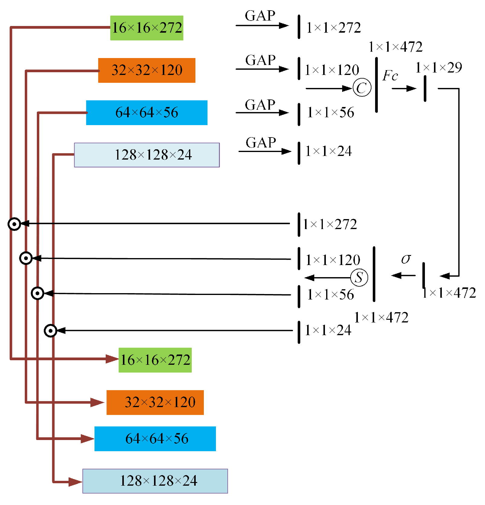
2.3. MFPN: An Enhanced Feature Extraction Neck for Robust Feature Fusion

The features obtained by the MNet include high-level features that have high semantic information but low-resolution and low-level features that have high-resolution but low semantic information. The role of the neck is to fuse these features to improve the ability of the model to extract information. For TPNet, we selected the FPN [50] architecture as the neck component and named it MFPN (MBlock FPN). The MFPN architecture integrates MBlock and PW convolution layers specifically designed to reduce parameter count and computational complexity. Additionally, we developed a new lightweight upsampling method. In this approach, the input features are first adjusted by MBlock to match the required number of output channels. Then, the spatial dimensions are expanded using bilinear interpolation, as illustrated in Figure 5.

To optimally harness the multi-scale features extracted from the backbone— encompassing rich semantic information in high-level features and abundant detailed information in low-level features—we introduced the DFRM, as depicted in Figure 6. The computational process is structured as follows:

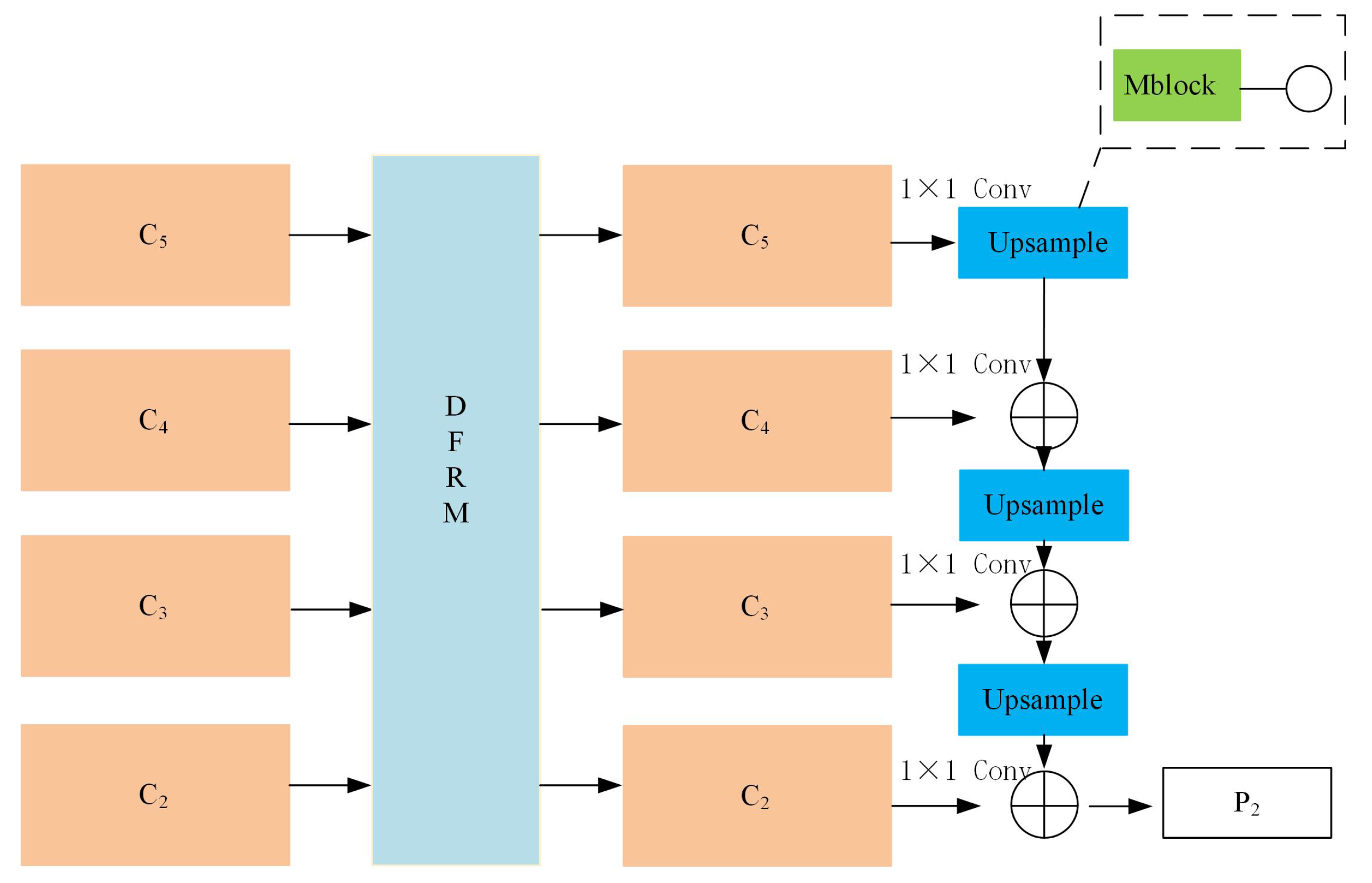
• Global information extraction: adaptive average pooling is applied to each feature map to capture global information. These global feature descriptors are subsequently concatenated and processed through lightweight convolutional layers to learn a set of weights.
• Weight calculation: the weights are derived via convolutional operations followed by a sigmoid activation function. These weights reflect the importance of each feature map in the current scene.
• Feature refinement: the refined features are obtained by channel-wise multiplication of the weights with the corresponding feature maps.

The calculation process is outlined below. Given multi-scale input features ${\{x_i\in {\mathbb{R}}^{C\times H_i\times W_i}\}}_{i=1}^N$, we generate channel descriptors through adaptive average pooling:

$$z_i={\mathcal{F}}_{\mathrm{gap}}\left(x_i\right)\in {\mathbb{R}}^{C\times 1\times 1}$$

(3)

The compressed features are concatenated and processed through lightweight convolutional layers to generate weights:

$$w=\sigma \left({\mathcal{F}}_{\mathrm{conv}}\left(\left[z_1,z_2,\dots ,z_N\right]\right)\right)\in {\mathbb{R}}^{N\times 1\times 1}$$

(4)

Finally, the refined features are obtained through channel-wise multiplication:

$${\widehat{x}}_i=w_i\odot x_i$$

(5)

Here, $\sigma$ denotes the sigmoid function, and ${\mathcal{F}}_{\mathrm{conv}}$ is implemented via lightweight convolutional layers.

This design enhances the model’s attention to critical features and improves the flexibility of the fusion process. By learning the weights, the model can automatically adjust its reliance on different feature maps, leading to better performance in complex and varied detection tasks. The ablation study of the DFRM is presented in Section 4.2.4.

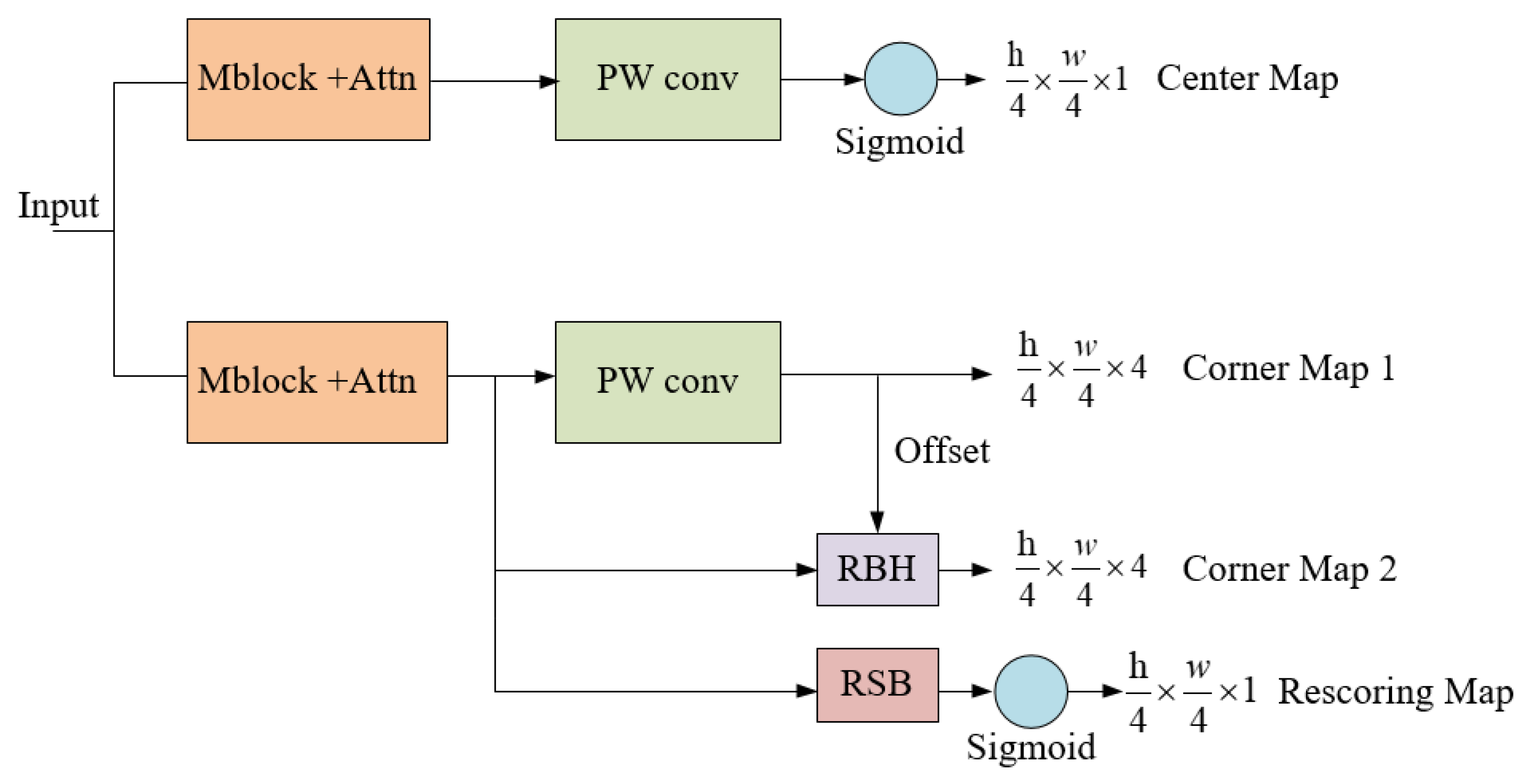
2.4. Detection Head Architecture and Output Components

In TPNet, the head component is composed of two distinct branches: the classification branch and the regression branch, as depicted in Figure 7. The classification branch produces the center map, which estimates the confidence score for each point, thereby determining the score assigned to the predicted bounding box at that location. The regression branch generates three outputs: corner map 1, corner map 2, and the rescoring map. The corner maps provide positional information for the predicted bounding boxes, while the rescoring map refines the center map’s predictions. Unlike CenterNet, TPNet determines the bounding box by predicting the horizontal and vertical distances from the center point to the upper-left and lower-right corners of the predicted box, as illustrated in Figure 2.

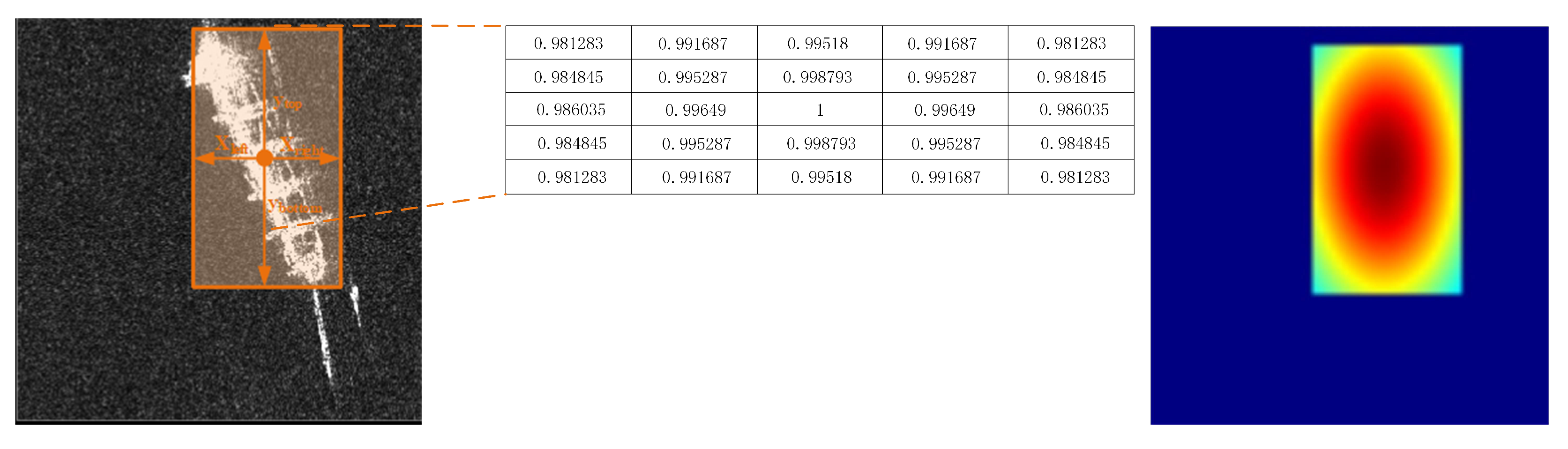
2.4.1. Center Map for Classification

The YOLO series employs the Intersection over Union (IoU) metric for label assignment. Specifically, an anchor is assigned a confidence level of 1 if its IoU with the true bounding box exceeds a predefined threshold, typically set at 0.7; otherwise, the confidence level is set to 0. In contrast, TPNet adopts a soft label strategy similar to that used in CenterNet. In this approach, the center point of the ship is assigned a label of 1, while the labels for surrounding points are determined according to Equation (6).

$$T_{xy}=e^{-\left({\displaystyle \frac{{\left(x-C_x\right)}^2}{2{\left({\sigma }_w\right)}^2}}+{\displaystyle \frac{{\left(y-C_y\right)}^2}{2{\left({\sigma }_h\right)}^2}}\right)}$$

(6)

Here, $T_{xy}$ refers to the assigned value at $(x,y)$, where $(x-C_x)$, $(y-C_y)$ denotes the distance from the center point, and ${\sigma }_h=0.5\times h$ and ${\sigma }_w=0.5\times w$ represent the standard deviations in height and width, respectively. Here, h and w denote the height and width of the target ship.

Figure 8 depicts a ship along with its corresponding ground truth heatmap on the center map.

Our classification branch employs the focal loss, as introduced by Zhou et al. [41], which is an enhancement of cross-entropy loss. The primary objective of focal loss is to address the problem of imbalanced sample ratios. In ship detection, the majority of image pixels or objects are classified as background, while only a small fraction corresponds to the ship class. This imbalance between positive and negative samples is thus pronounced. The formula for calculating the loss in the classification branch is given by:

$$L_{cls}={\displaystyle \frac{-1}{N}}\sum _{xy}\left\{\begin{array}{cc}{\left(1-P_{xy}\right)}^{\alpha }log\left(P_{xy}\right)\hfill & T_{xy}=1\hfill \\ {\left(1-T_{xy}\right)}^{\beta }{\left(P_{xy}\right)}^{\alpha }log\left(1-P_{xy}\right)\hfill & \mathrm{otherwise}\hfill \end{array}\right.$$

(7)

where $T_{xy}$ represents the ground truth and $P_{xy}$ means the output of the center map, $\alpha$ = 2, $\beta$ = 6, and N denotes the number of ships in the image.

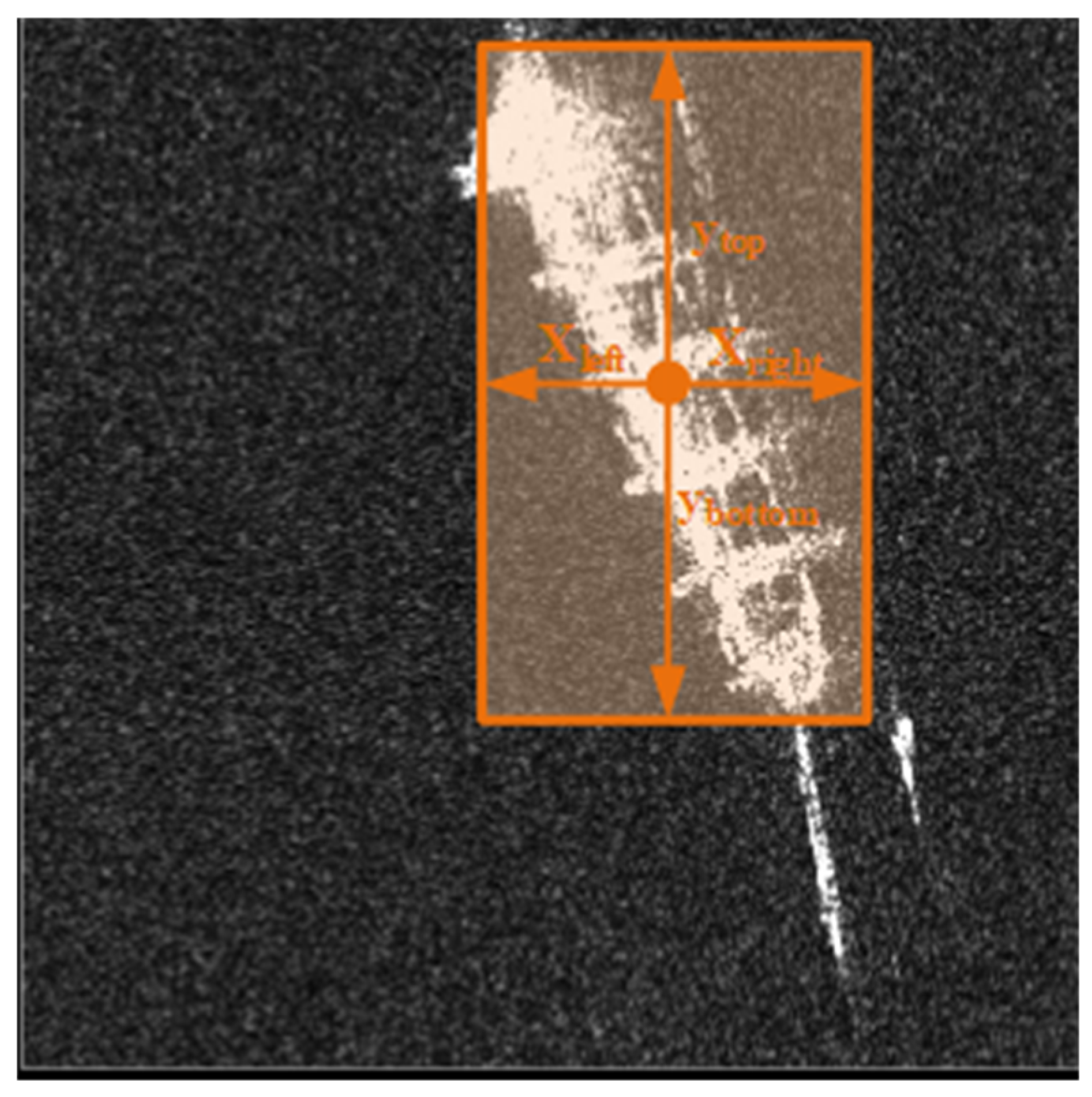
2.4.2. Corner Map1 for Localization

As illustrated in Figure 2, in TPNet, the bounding box of a ship is determined by four distances $X_{left}$$Y_{top}$$X_{right}$$Y_{bottom}$, as well as the coordinate of the center point, which is determined by the center map. Specifically, if a point ($x_0,y_0$) on the center map has a value exceeding a predefined threshold (0.1), it is identified as the center point of a ship. The bounding box for the ship can then be determined using the following formula:

$$\begin{array}{cc}\hfill & x_1=DR\times (x_0-l)=DR\times \left(x_0-e^{c_1\left(x_0,y_0\right)}\right)\hfill \\ \hfill & y_1=DR\times (y_0-t)=DR\times \left(y_0-e^{c_2\left(x_0,y_0\right)}\right)\hfill \\ \hfill & x_2=DR\times (x_0+r)=DR\times \left(x_0+e^{c_3\left(x_0,y_0\right)}\right)\hfill \\ \hfill & y_2=DR\times (x_0+b)=DR\times \left(y_0+e^{c_4\left(x_0,y_0\right)}\right)\hfill \end{array}$$

(8)

here DR represents the downsample ratio, and $c_k(x_0,y_0)$ denotes the output of the k-th channel of the corner map1 at the coordinates $(x_0,y_0)$.

2.4.3. Corner Map2 for Refining Bounding Box

Bounding box regression is a critical component of object detection, aimed at leveraging center point information for accurate regression. However, due to the effects of downsampling, the projection of the center point onto the feature map is typically non-integer, necessitating the use of information from the nearest integer coordinates rather than the center point itself. This limitation highlights the need for a more effective method to better utilize center point information to enhance the precision of bounding box regression, leading to the development of deformable convolution [55].

Unlike traditional convolution operations, deformable convolutions enhance object detection accuracy by learning deformation information to adapt to variations in object shapes. The core of deformable convolution is the deformable module, which comprises an offset prediction module and a sampling module. The offset prediction module learns the displacement of each pixel, while the sampling module uses these offsets to sample the input feature map. The formula for deformable convolution is as follows:

$$Y\left(p_0\right)=\sum _{p_i\in R}w\left(p_i\right)·X(p_0+p_i+\Delta p_i)$$

(9)

In this equation, $Y\left(p_0\right)$ represents the output feature map at position $p_0$, X denotes the input feature map, $w\left(p_i\right)$ is the weight at position $p_i$ in the convolution kernel, and $\Delta p_i$ refers to the learned offsets that enable the convolution to adapt to the shape of the object. These offsets are derived through

Table 2. Offsets employed in RBH.

Position	Coordinates
Center	$(0,0)$
Left	$(-l,0)$
Right	$(r,0)$
Top	$(0,t)$
Bottom	$(0,b)$
Top-Left	$(-l,-t)$
Top-Right	$(r,-t)$
Bottom-Left	$(-l,b)$
Bottom-Right	$(r,b)$

$l,t,r,b$ are concluded from Equation (8).

in this article.

Given a sampling location $(x_0,y_0)$ on the feature map, TPNet regresses an initial bounding box from this location using Equation (8). Utilizing the distance vector $(l,t,r,b)$, we can obtain nine sampling points: Center, Left, Right, Top, Bottom, Top-Left, Top-Right, Bottom-Left, Bottom-Right by Table 2 and map these points onto the feature map. The relative offsets of these points to the projection point $(x_0,y_0)$ serve as the offsets for the deformable convolution. Since these points are manually calculated, there is no additional prediction burden, making this operation computationally more efficient compared to traditional deformable convolutions.

To enhance the accuracy of bounding box regression, the RBH module is introduced, as illustrated in Figure 9. The RBH module operates as a 3 × 3 deformable convolution, with its offsets derived from the output of the corner map1, as specified by Equation (2), distinguishing it from conventional deformable convolutions. The input to the RBH module is identical to that of corner map1, meaning both receive the feature maps produced by the regression branch, which contains extensive localization information. After applying the RBH module, the bounding box can be adjusted using Equation (10):

$$\begin{array}{cc}\hfill & x_1=DR\times \left(x_0-e^{c_1\left(x_0,y_0\right)}+r_1\left(x_0,y_0\right)\right)\hfill \\ \hfill & y_1=DR\times \left(y_0-e^{c_2\left(x_0,y_0\right)}+r_2\left(x_0,y_0\right)\right)\hfill \\ \hfill & x_2=DR\times \left(x_0+e^{c_3\left(x_0,y_0\right)}+r_3\left(x_0,y_0\right)\right)\hfill \\ \hfill & y_2=DR\times \left(y_0+e^{c_4\left(x_0,y_0\right)}+r_4\left(x_0,y_0\right)\right)\hfill \end{array}$$

(10)

$r_k(x_0,y_0)$ represents the output of the k-th channel of the RBH module at the coordinates $(x_0,y_0)$. The ablation studies presented in Section 4.2.5 will illustrate that the RBH module can effectively enhance the detection accuracy of TPNet.

2.4.4. RSB for Refining Center Map

In TPNet, the center map and corner map are responsible for predicting the confidence scores and bounding boxes, respectively, and they are trained using distinct loss functions without clear mutual awareness. Consequently, while the center map predicts the confidence of each bounding box, it lacks information about the corresponding localization quality. The standard measure for evaluating the localization quality of a bounding box is its Intersection over Union (IoU) with the ground truth box. Therefore, the scores obtained from the center map can easily mismatch with the localization accuracy. For instance, some high-quality predicted boxes may be deleted because of their low scores in the center map, or some predicted boxes with poor localization accuracy may be retained because of their high scores in the center map. This phenomenon can negatively impact the detector’s performance: during Non-Maximum Suppression (NMS), predicted boxes are ranked according to their center map scores, leading to high-scoring boxes suppressing other overlapping boxes. This can lead to the removal of high-quality predictions and the retention of low-quality ones, which is particularly detrimental given TPNet’s goal of accurately predicting target ships.

To tackle the aforementioned problem of localization accuracy in object detection, inspired by the IoU-aware detector [56], a novel approach named Refining Score Branch (RSB) is proposed. RSB is incorporated into the final layer of the regression branch to predict the IoU of each regressed anchor. During the training phase, RSB is jointly trained with the classification and regression branches, the cost function for RSB is Equation (11). During inference, the center map is calibrated by multiplying the rescoring map, which is the output of the RSB. To maintain computational efficiency, RSB consists of a single 1 × 1 convolution layer followed by a sigmoid activation function to ensure the predicted IoU falls within the range [0, 1]. RSB adds minimal computational burden to the entire model while still substantially enhancing its performance.

$$L_{RSB}=-{\displaystyle \frac{1}{N}}\sum _{i=1}^N\left[y_i·log\left(p_i\right)+(1-y_i)·log(1-p_i)\right]$$

(11)

here N is the number of positive points, $y_i$ is the IoU between the predicted bounding box and the ground truth box at point i, and $p_i$ is the corresponding predicted score in the rescoring map at that point i. The ablation study of the RSB will be presented in Section 4.2.6.

2.5. WGIoU Loss Function

The CenterNet object detection framework utilizes a regression loss based on the Smooth L1 loss; however, Smooth L1 loss has several drawbacks that can limit its effectiveness in certain situations. For instance, it may result in slower convergence and is highly sensitive to hyperparameter tuning. Furthermore, it treats the four distances used for bounding box regression as independent variables, although they are inherently correlated.

To address these limitations, TPNet utilizes the Generalized Intersection over Union (GIoU) to measure the similarity between predicted and ground truth bounding boxes. GIoU considers the overlap between the predicted and ground truth boxes, making it more effective than Smooth L1 loss, particularly in scenarios where the bounding boxes are either very small or very large.

After investigating the regression loss employed by FCOS and CenterNet, we observed that both methods consider only positive samples in their regression loss, i.e.,

$$los{s}_{reg}={\displaystyle \frac{1}{N_{\mathrm{pos}}}}\sum _{x,y}{l}_{reg}(box1,box2)$$

(12)

where the points are positive samples in the regression branch.

However, we are of the belief that “negative” samples in close proximity to the center of the object also play a role in enhancing the accuracy of bounding box predictions. Hence, a weighting parameter is indispensable to mirror the significance of each predicted value. To resolve this problem, we put forward the WGIoU loss. This loss function utilizes the values from the center map as weights, taking into consideration the varying importance of each prediction point. The WGIoU loss takes into account the “centerness” of each sample and modifies the GIoU loss correspondingly to reflect its importance in the localization process. It represents an improvement over the GIoU loss. The  computation process of the wGIoU loss is as in Algorithm 1.

By combining Equations (7) and (11) with Algorithm 1, we can obtain the total loss function of TPNet, which is represented as

$$loss\_total=loss\_cls+loss\_box+loss\_RSB$$

(13)

The $loss\_cls$ term is responsible for classification, the $loss\_box$ term handles bounding box regression, and the $loss\_RSB$ term optimizes the RSB. The purpose of this loss function is to train the network to accurately classify and localize ships within the input images.

Algorithm 1 The calculation process of WGIoU loss

Input: Center map: ${\mathit{C}}_{\mathit{1}}\in {\mathbb{R}}^{H\times W\times 1}$, Corner map1: ${\mathit{C}}_{\mathit{1}}\in {\mathbb{R}}^{H\times W\times 4}$, Corner map2: ${\mathit{C}}_{\mathit{2}}\in {\mathbb{R}}^{H\times W\times 4}$ Output: $\mathit{loss}\_\mathit{box}$      1: $loss1=0$, $loss2=0$, $\mathit{avg}\_\mathit{factor}=0$      2: for all every point $(i,j)$ do      3:     if $\mathit{C}(i,j)>0$ then      4:         get box1 predicted by corner map1 by Equation (8)      5:         get box2 predicted by corner map1 and corner map2 by Equation (10)      6:         get the ground truth bounding box from the annotation file denoted as $\mathrm{true}\text{\_}\mathrm{box}$      7:         compute the GIoU between box1 and the $\mathrm{true}\text{\_}\mathrm{box}$ ($giou1$), as well as the GIoU between box2 and the $\mathrm{true}\text{\_}\mathrm{box}$ ($giou2$)      8:         $loss1+=\mathit{C}(i,j)\times (1-giou1)$, $loss2+=\mathit{C}(i,j)\times (1-giou2)$      9:         $\mathit{avg}\_\mathit{factor}+=\mathit{C}(i,j)$     10:     end if     11: end for     12: $\mathit{loss}\_\mathit{box}=(loss1+loss2)/\mathit{avg}\_\mathit{factor}$     13: return $\mathit{loss}\_\mathit{box}$

2.6. WSE Attention Module

In complex environmental conditions, accurately detecting ships can be challenging due to the similarity in backscattering characteristics between ships and the background. Attention mechanisms offer a viable solution to this problem by enhancing the feature extraction capabilities of detection algorithms. These mechanisms enable the detector to focus on key features, thereby improving the accuracy and robustness of ship detection. Moreover, attention modules are generally lightweight, allowing for effective ship detection in complex backgrounds without compromising detection speed.

The introduction of attention modules to computer vision was pioneered by SENet [57]. This layer employs a straightforward yet effective mechanism to adaptively recalibrate channel-wise feature responses by explicitly modeling interdependencies between channels. Since its inception, the SE layer has become a cornerstone in modern deep neural network design, achieving state-of-the-art performance across various computer vision tasks, including SAR ship detection [30]. The SE layer has inspired the development of numerous attention models, including the Convolutional Block Attention Module (CBAM) [58], Coord Attention (CA) [59], Efficient Channel Attention (ECA) module [60] and effective Squeeze-and-Excitation (eSE) [61].

Despite these advancements, we found that channel attention mechanisms, such as SE layers, do not incorporate positional information. While CBAM considers positional information, it processes it separately from channel information. On the other hand, self-attention modules like the Non-Local module [62] address both channel and positional information but involve a complex computational process, which does not align with our objective of achieving fast and lightweight ship detection.

To develop a lightweight and efficient attention module, we first examine the channel attention mechanism used in SENet. As detailed in Equations (14) and (15), SENet applies a global average pooling operation on a per-channel basis, followed by two fully connected (FC) layers with non-linear activation functions. A Sigmoid function is then used to generate channel weights. The purpose of these FC layers is to capture non-linear cross-channel interactions while reducing model complexity through dimensionality reduction. However, we identified a key limitation of the SE layer: the use of average pooling does not account for positional information and instead averages across all positions within a channel.

To address this limitation, we propose an enhancement to the original Equation (15), referred to as Equation (16). This enhancement allows for the representation of the importance of each position within a channel. WSE enhances the SE module by adaptively assigning weights to different spatial locations. The modified Equation (16) is integrated with Equation (14) to define the WSE layer, which is an improvement over the traditional SE module. WSE incorporates both spatial and channel-wise attention mechanisms. The computation process for the WSE layer is detailed in Algorithm 2.

Algorithm 2 The calculation process of the WSE layer

Input: Tensor $\mathit{X}:\in {\mathbb{R}}^{H\times W\times C}$ Output: Tensor $\mathit{Y}:\in {\mathbb{R}}^{H\times W\times C}$ Require: a 1x1 convolutional layer conv whose input channels is C and output channels is 1, and two FC layers fc1 and fc2       1: $\mathit{w}(i,j)=\mathrm{softmax}\left(\mathrm{conv}\right(\mathit{X}\left)\right)$       2: $\mathit{scale}={\sum }_{i=1}^H{\sum }_{j=1}^W\mathit{w}(i,j)·\mathit{x}(i,j,k)$       3: $\mathit{scale}=\mathrm{fc}2\left(\mathrm{fc}1\right(\mathit{scale}\left)\right)$       4: $\mathit{scale}=\mathrm{sigmoid}\left(\mathit{scale}\right)$       5: $\mathit{Y}=\mathit{scale}·\mathit{X}$       6: return $\mathit{Y}$

$$f_s=\sigma \left(\mathrm{FC}\left(ReLU\left(\mathrm{FC}\left(f_g\right)\right)\right)\right)$$

(14)

while $f_g$ can be calculated by:

$$f_g={\displaystyle \frac{1}{H\times W}}\sum _{i=1}^H\sum _{j=1}^{W}x(i,j)$$

(15)

in WSE, $f_g^{\prime }$ can be rewritten as follows:

$$f_g^{\prime }=\sum _{i=1}^H\sum _{j=1}^{W}w(i,j)·x(i,j)$$

(16)

where $w(i,j)$ measures the importance of each point, with the constraint that ${\sum }_{i=1}^H{\sum }_{j=1}^W$$w(i,j)=1$. Notably, the SE mechanism is a special case of the WSE layer, where $w(i,j)={\displaystyle \frac{1}{H\times W}}$.

2.7. The Workflow of TPNet

The entire pipeline for TPNet to process an image is as follows:

• Step 1: Pre-process the detected image and feed the pre-processed image to MNet. The features generated by MNet are further processed by the neck to obtain a feature map, then this feature map is fed to the Head.
• Step 2: As shown in Figure 7, the Head generates a center map, a corner map1, a corner map2, and a rescoring map. The final center map is obtained by multiplying the center map and the rescoring map. Points on the center map with values greater than the set threshold (0.1) are identified as positive and recorded as ($x_0$, $y_0$), ($x_1$, $y_1$), etc.
• Step 3: Using Equation (10) and the corner map1 and corner map2, bounding boxes corresponding to these points are obtained and recorded as $(x_{1}0,y_{1}0,x_{2}0,y_{2}0)$, $(x_{1}1,y_{1}1,x_{2}1,y_{2}1)$, etc.
• Step 4: The bounding boxes from Corner map2 and their corresponding scores on the refined center map are integrated and processed through NMS to yield the final predicted ships.

3. Experiment Settings

To assess TPNet’s performance, we designed a comprehensive experimental program, comparing it with 14 state-of-the-art CNN-based detection algorithms. Our experimental framework includes dataset construction, evaluation metric design, comparative algorithm selection, and ablation experiments.

3.1. Datasets

We perform experiments on three publicly available datasets, namely SAR-Ship-Dataset [63], SSDD [23] and HRSID [64]; the characteristics of these three datasets are presented in

Table 3. Basic information of SAR-ship-dataset, SSDD and HRSID.

Dataset	Num of Images	Num of Ships	Satellites	Resolution (m)
SAR-ship-dataset	43,819	59,535	GF3 Sentinel-1	5–20
SSDD	5604	16,951	TerraSAR-X Sentinel-1 RadarSat-2	1–10
HRSID	1160	2540	TerraSAR-X Sentinel-1B TanDEM	0.5–3

.

The SAR-Ship Dataset comprises 43,819 images featuring a total of 59,535 ships. Each image has dimensions of 256 × 256 pixels and is cropped from GF-3 and Sentinel-1 satellite images. The dataset includes images with resolutions ranging from 3 m to 22 m and covers various polarization modes such as HH, HV, VH, and VV. It encompasses a broad range of maritime scenes, including ports, inshore areas, islands, and offshore environments. The ships in the dataset include various types, such as oil tankers, bulk carriers, large container ships, and fishing vessels. The dataset is divided into training and testing subsets with an 80:20 ratio, resulting in 35,055 samples for training and 8764 samples for testing. Figure 10 describes the ship size distribution in the SAR-Ship Dataset.

The SSDD is the first publicly available SAR ship detection dataset; it contains a total of 1160 SAR images, which have an average size of 400 × 400 pixels and are obtained from Sentinel-1, TerraSAR-X, and RadarSat-2. The dataset provides SAR images of ships at various resolutions, ranging from 1m to 10m, and from different polarizations, including HH, HV, VV, and VH. Furthermore, the dataset includes a wide variety of ship sizes, ranging from the smallest size of 7 × 7 to the largest size of 211 × 298 pixels, which can be used to evaluate the multi-scale detection performance of different models.

The HRSID dataset consists of 5,604 SAR, each with a resolution of 800 × 800 pixels, acquired from the Sentinel-1 and TerraSAR-X satellites. The dataset provides SAR ship targets with resolutions ranging from 0.1 m to 3 m, and includes three different polarization modes: HH, HV, and VV.

It is noteworthy that unlike other researchers, we did not partition the SSDD and HRSID datasets into separate training and test sets. Instead, we directly used them as the test set to evaluate the performance of the detector trained on the SAR-Ship-Dataset training set. This approach was adopted to demonstrate the superior generalization ability of TPNet.

3.2. Evaluation Metrics

We utilized six evaluation metrics: ${\mathrm{AP}}_{50}$, ${\mathrm{AP}}_{75}$, AP, ${\mathrm{AP}}_{\mathrm{small}}$, ${\mathrm{AP}}_{\mathrm{medium}}$, and ${\mathrm{AP}}_{\mathrm{large}}$—to comprehensively assess the detection accuracy of our detector. In addition, we evaluated the computational complexity of various algorithms using the FLOPs metric and measured the detection speed of the algorithms using FPS (Frames Per Second).

3.3. Experimental Environment, and Implementation Details

The experiments were conducted on a computer equipped with an i9-9900K CPU and Tesla V100 GPU, and PaddlePaddle was utilized for the implementation. To ensure a fair comparison, TPNet and the other 14 advanced SAR ship detectors were implemented using the PaddleDetection 2.6 toolbox [65]. It is worth noting that in our work, we did not utilize any pretrained weights for TPNet, and instead trained it from scratch.

During training, we utilized the AdamW optimizer with a regularizer factor of 0.001. The initial learning rate was set to 0.01 with a warm-up period of 2000 iterations. After the warm-up, a cosine learning rate schedule was employed. All models were trained on the training set of the SAR-Ship-Dataset for 36,000 iterations with a batch size of 64. To improve the training process, we also adopted the exponential moving average (EMA) strategy with a decay rate of 0.9998. To further augment our training data, we employed various techniques such as random flipping, random expansion, and random cropping.

4. Experimental Results

4.1. Comparative Experiments

To evaluate the performance of TPNet, we selected 14 advanced CNN-based detectors for comparison: YOLOv3 [16], YOLOv4 [17], YOLOv5 [18], YOLOv7 [66], YOLOv8 [67], YOLOv10 [68], YOLOv11 [67], PP-YOLO [20], PP-YOLOv2 [21], PP-YOLOE [22], RetinaNet [69], CenterNet [41], FCOS [42], and TTFNet [70]. All detectors, including TPNet, were trained using the same methodology to ensure a fair comparison.

4.1.1. Visualization of Detection Results

Figure 11 presents the detection results of six selected detectors on five SAR images, where blue, green, and red bounding boxes represent correct, missed, and false detections, respectively. The chosen detectors include our proposed TPNet, PP-YOLO-v2 (second-best performing algorithm in terms of AP), YOLOv3 (a classic YOLO algorithm), YOLOv10 and YOLOv11 (state-of-the-art YOLO algorithms), and CenterNet (the foundational algorithm that inspired our work). We selected five typical scenarios: the first column illustrates offshore ship detection in simple backgrounds, while columns two to five depict inshore ship detection in complex scenarios. The complete detection results for all 15 algorithms are provided in Figure A1.

From Figure 11, the following conclusions can be drawn: most detection algorithms can easily identify offshore ships in simple scenes but struggle with inshore ships in complex environments, leading to missed and false detections. Compared to other algorithms, TPNet excels in handling complex-background ship detection. For instance, in the last column, although PP-YOLOv2 match TPNet’s detection accuracy, PP-YOLOv2 underperforms TPNet in the second and third columns. This highlights TPNet’s superior accuracy in complex scenarios.

4.1.2. Comparison of Experimental Results

In the previous subsection, we conducted a qualitative analysis of the detection effects of various algorithms, revealing their performance differences in practical applications. However, visual assessment alone cannot comprehensively and accurately evaluate algorithm superiority. To precisely assess TPNet’s advantages and limitations compared to other advanced algorithms, this section delves into quantitative analysis. We quantitatively compare algorithm detection performance using widely-recognized metrics: ${\mathrm{AP}}_{50}$, ${\mathrm{AP}}_{75}$, AP, ${\mathrm{AP}}_{\mathrm{small}}$, ${\mathrm{AP}}_{\mathrm{medium}}$, and ${\mathrm{AP}}_{\mathrm{large}}$. Moreover, considering computational resource constraints in real-world applications, we include computational complexity (measured by FLOPs) to evaluate the balance between performance and efficiency. Experimental results are shown in

Table 4. Test results of different algorithms on SAR-Ship-Dataset.

Algorithm	AP50 (%)	AP75 (%)	AP (%)	APsmall (%)	APmiddle (%)	APlarge (%)	FLOPs (G)	FPS
YOLOv3 [16]	94.6	60.7	55.8	51.9	61.4	55.9	12.377	302.2
YOLOv4 [17]	91.6	53.4	51.6	46.9	58.0	54.3	9.766	300.5
YOLOv5 [18]	94.1	66.1	58.2	54.0	66.4	53.0	8.637	298.7
YOLOv7 [66]	84.3	48.2	47.2	42.5	54.2	25.6	8.391	293.2
YOLOv8 [67]	93.2	64.2	57.7	53.2	64.0	59.6	15.378	305.7
YOLOv10 [68]	93.7	67.5	59.2	54.6	65.9	63.8	9.632	233.7
YOLOv11 [67]	93.4	65.5	58.1	53.6	64.5	59.1	14.664	297.1
PP-YOLO [20]	92.6	62.3	55.9	51.2	62.5	63.6	9.153	300.0
PP-YOLOv2 [21]	94.7	70.1	60.3	56.0	66.5	63.7	9.153	303.7
PP-YOLOE [22]	93.8	66.8	59.2	54.5	66.0	65.0	8.879	298.9
RetinaNet [69]	80.2	34.1	39.5	31.4	51.6	43.8	12.988	103.6
CenterNet [41]	91.8	55.1	52.8	46.5	61.4	73.6	6.433	38.7
TTFNet [70]	92.7	64.5	57.6	51.9	65.2	69.4	11.931	119.4
FCOS [42]	90.0	56.9	52.9	44.9	63.7	52.6	12.865	298.0
TPNet	95.7	71.4	62.1	56.4	69.3	73.3	0.485513	316.9

. Through systematic analysis of these quantitative indicators, we aim to present a clear and objective overview of algorithm performance, thereby more strongly supporting our conclusions.

Based on the results presented in Table 4, we can draw the following conclusions:

TPNet is an exceptionally lightweight network, requiring only 7.54% of the computational cost of CenterNet. In terms of speed, TPNet is also the fastest among the 15 algorithms. Despite its low computational cost, TPNet achieves high detection accuracy. Specifically, TPNet outperforms 14 other detection algorithms across five out of six metrics: ${\mathrm{AP}}_{50}$, ${\mathrm{AP}}_{75}$, AP, ${\mathrm{AP}}_{\mathrm{small}}$, and ${\mathrm{AP}}_{\mathrm{middle}}$. The only exception is ${\mathrm{AP}}_{\mathrm{large}}$, where TPNet demonstrates strong performance but does not lead. In terms of ${\mathrm{AP}}_{50}$, TPNet exceeds the second-best PP-YOLOv2 by 1% and the third-best YOLOv3 by 1.1%. For ${\mathrm{AP}}_{75}$, TPNet surpasses PP-YOLOv2 by 1.3% and leads the third-best algorithm YOLO v10 by 3.9%. This performance demonstrates TPNet’s superior localization accuracy in addition to its ship detection capabilities. The AP metric, which measures average detection performance across different IoUs, is widely regarded as a crucial indicator of detector performance. TPNet outperforms PP-YOLOv2 by 1.8% and PP-YOLOE/YOLO v10 by 2.9% in this metric. In the detection of small ships (${\mathrm{AP}}_{\mathrm{small}}$), TPNet leads PP-YOLOv2 by 0.4% and YOLO v10 by 1.8%, demonstrating its effectiveness in detecting smaller targets. Moreover, TPNet excels in the detection of medium-sized ships, with its ${\mathrm{AP}}_{\mathrm{middle}}$ exceeding PP-YOLOv2 by 2.8% and YOLOv5 by 2.9%. Although TPNet ranks behind CenterNet in ${\mathrm{AP}}_{\mathrm{large}}$, it still achieves a strong second-place ranking among the 15 algorithms tested, indicating solid performance in detecting large ships.

Many researchers train and test their detection algorithms on the same dataset. While this approach provides a useful benchmark for comparison, we argue that robust object detection algorithms should demonstrate strong generalization ability. An effective algorithm should learn fundamental features from the training dataset, enabling it to perform well on other datasets. To assess this capability, we evaluated the performance of detectors trained on the SAR-Ship-Dataset’s training set using two additional widely used open-source SAR ship detection datasets: HRSID and SSDD. The results of these evaluations are presented in

Table 5. Test results of different algorithms on HRSID.

Algorithm	AP50 (%)	AP75 (%)	AP (%)	APsmall (%)	APmiddle (%)	APlarge (%)
YOLOv3 [16]	69.1	41.9	40.1	43.4	24.7	1.1
YOLOv4 [17]	71.1	41.7	40.2	43.4	28.1	1.1
YOLOv5 [18]	65.9	40.5	38.6	42.4	19.5	0.0
YOLOv7 [66]	64.1	41.9	37.9	41.1	22.0	0.0
YOLOv8 [67]	71.2	47.0	43.1	47.2	25.4	0.1
YOLOv10 [68]	71.5	49.4	44.3	48.0	28.7	0.8
YOLOv11 [67]	72.4	49.3	44.5	48.5	28.6	0.3
PP-YOLO [20]	59.7	38.5	35.4	38.7	20.8	0.2
PP-YOLOv2 [21]	70.7	45.5	42.2	45.8	26.1	0.4
PP-YOLOE [22]	69.6	47.9	43.2	46.3	34.8	2.5
RetinaNet [69]	59.4	25.3	29.1	31.7	24.0	0.2
CenterNet [41]	70.4	44.9	41.9	44.9	29.4	0.9
TTFNet [70]	73.2	46.3	43.3	46.8	27.1	0.1
FCOS [42]	55.8	15.9	24.3	31.0	14.8	0.1
TPNet	71.0	47.7	43.3	46.6	35.5	0.3

,

Table 6. Test results of different algorithms on SSDD.

Algorithm	AP50 (%)	AP75 (%)	AP (%)	APsmall (%)	APmiddle (%)	APlarge (%)
YOLOv3 [16]	77.7	28.9	37.2	35.9	40.7	26.6
YOLOv4 [17]	78.9	29.5	37.4	36.8	40.3	20.3
YOLOv5 [18]	45.9	10.6	18.6	18.8	19.6	3.5
YOLOv7 [66]	72.5	33.1	36.6	33.1	37.5	38.2
YOLOv8 [67]	78.4	30.6	38.1	38.0	40.5	12.2
YOLOv10 [68]	82.5	34.3	40.3	39.9	42.9	21.1
YOLOv11 [67]	78.3	32.4	38.5	38.3	40.9	16.3
PP-YOLO [20]	82.9	36.8	41.6	40.5	45.0	23.2
PP-YOLOv2 [21]	79.6	34.7	39.7	38.0	43.5	29.2
PP-YOLOE [22]	71.9	30.8	35.6	29.5	45.8	38.8
RetinaNet [69]	74.4	23.8	33.6	33.8	36.2	20.9
CenterNet [41]	75.5	31.0	37.1	35.5	41.7	16.8
TTFNet [70]	74.6	25.3	34.1	34.7	35.0	11.5
FCOS [42]	69.2	17.3	28.7	29.4	30.7	19.4
TPNet	86.1	44.2	45.9	44.1	50.8	21.6

and

Table 7. Combined test results of different algorithms on HRSID and SSDD.

Algorithm	AP50 (%)	AP75 (%)	AP (%)	APsmall (%)	APmiddle (%)	APlarge (%)
YOLOv3 [16]	146.8	70.8	77.3	79.3	65.4	27.7
YOLOv4 [17]	150.0	71.2	77.6	80.2	68.4	21.4
YOLOv5 [18]	111.8	51.1	57.2	61.2	39.1	3.5
YOLOv7 [66]	136.6	75.0	74.5	74.2	59.5	38.2
YOLOv8 [67]	149.6	77.6	81.2	85.2	65.9	12.3
YOLOv10 [68]	154.0	83.7	84.6	87.9	71.6	21.9
YOLOv11 [67]	150.7	81.7	83.0	86.8	69.5	16.6
PP-YOLO [20]	142.6	75.3	77.0	79.2	65.8	23.4
PP-YOLOv2 [21]	150.3	80.2	81.9	83.8	69.6	29.6
PP-YOLOE [22]	141.5	78.7	78.8	75.8	80.6	41.3
RetinaNet [69]	133.8	49.1	62.7	65.5	60.2	21.1
CenterNet [41]	145.9	75.9	79.0	80.4	71.1	17.7
TTFNet [70]	147.8	71.6	77.4	81.5	62.1	11.6
FCOS [42]	125.0	33.2	53.0	60.4	72.5	19.5
TPNet	157.1	91.9	89.2	90.7	86.3	21.9

.

Based on the results presented in Table 5, Table 6 and Table 7, we can draw the following conclusions:

When assessing performance via the ${\mathrm{AP}}_{50}$ metric, algorithm performances varied across datasets. TTFNet shone on the HRSID dataset but had average results on the SSDD dataset. In contrast, TPNet excelled on the SSDD dataset and performed strongly on HRSID. Overall, for the ${\mathrm{AP}}_{50}$ metric considering both datasets, TPNet was the top-performer. Regarding the ${\mathrm{AP}}_{75}$ metric, YOLO v10 was outstanding on the HRSID dataset yet underperformed on the SSDD dataset. Conversely, TPNet not only led in performance on the SSDD dataset but also did quite well on HRSID. Across both datasets, TPNet had overall superiority in the ${\mathrm{AP}}_{75}$ metric, making it the most effective algorithm. Evaluated by the AP metric, YOLO v11 achieved top performance on the HRSID dataset. However, on the SSDD dataset, its performance paled in comparison to TPNet. In contrast, TPNet consistently outperformed other algorithms on the SSDD dataset and was highly competitive on HRSID. Considering both datasets, TPNet emerged as the leading algorithm in terms of the AP metric, showing superior and more stable performance across different scenarios. For the ${\mathrm{AP}}_{\mathrm{small}}$ metric, YOLOv11 had superior performance on the HRSID dataset but underperformed on the SSDD dataset. TPNet, meanwhile, performed strongly on both datasets. Considering both, TPNet was the leading algorithm for the ${\mathrm{AP}}_{\mathrm{small}}$ metric. When evaluated using the ${\mathrm{AP}}_{\mathrm{middle}}$ metric, TPNet achieved the highest performance on both datasets, firmly establishing itself as the optimal algorithm for this detection metric. With the ${\mathrm{AP}}_{\mathrm{large}}$ metric, the PP-YOLOE algorithm outperformed all others on both datasets. TPNet’s performance on this metric was less impressive, suggesting areas for improvement in detecting large ships. Overall, considering performance across both datasets and all six metrics, TPNet demonstrated the best generalization ability among the 15 detectors evaluated.

4.2. Ablation Experiments

To evaluate the effectiveness of the six proposed mechanisms and understand their impact on TPNet’s performance, we conducted a series of ablation experiments, as shown in the following subsections.

4.2.1. Ablation Experiments on Downsample Ratio

Figure 10 shows the size statistics of all ships in the training set of the SAR-Ship dataset. It can be seen that the majority of the ships have length and width smaller than 50, which means they are small or medium-sized targets. To improve the detection performance on these ships, we chose the feature map with a downsampling ratio of 4 for ship detection. Meanwhile, we also conducted a comparative experiment using the feature map with a downsampling ratio of 8, and the experimental results are shown in

Table 8. Test results on different datasets under different $DR$ values.

Dataset	DR	AP50 (%)	AP75 (%)	AP (%)	APsmall (%)	APmiddle (%)	APlarge (%)	FLOPs (G)
SAR-Ship Dataset	4	95.7	71.4	62.1	56.4	69.3	73.3	0.485513
	8	94.9	67.6	59.5	54.0	67.8	61.1	0.378620
HRSID	4	71.0	47.7	43.3	46.6	35.5	0.3	-
	8	63.7	32.5	33.7	37.6	25.2	0.0	-
SSDD	4	86.1	44.2	45.9	44.1	50.8	21.6	-
	8	84.4	34.8	41.4	40.4	44.6	22.7	-
HRSID and SSDD	4	157.1	91.9	89.2	90.7	86.3	21.9	-
	8	148.1	67.3	75.1	78.0	69.8	22.7	-

.

Table 8 demonstrates that utilizing high-resolution feature maps can significantly enhance detection performance, particularly in the ${\mathrm{AP}}_{75}$ metric. This indicates that high-resolution feature maps provide richer positional information, leading to more accurate bounding boxes. Additionally, the results on HRSID and SSDD, as shown in Table 8, indicate that TPNet with a $DR$ value of 4 exhibits superior generalization performance compared to TPNet with a $DR$ value of 8. Therefore, in this study, we selected $DR$ = 4.

4.2.2. Ablation Experiments on MBlock

In order to reduce the computational cost of the model, we designed a lightweight module, MBlock, to replace the traditional convolution module. We conducted ablation experiments to evaluate the performance of MBlock, and the results are shown in

Table 9. Test results on different datasets under different operators.

Dataset	Operator	AP50 (%)	AP75 (%)	AP (%)	APsmall (%)	APmiddle (%)	APlarge (%)	FLOPs (G)
SAR-Ship Dataset	Traditional Convolution	95.2	70.0	61.0	54.9	68.7	63.9	1.000
	MBlock	95.7	71.4	62.1	56.4	69.3	73.3	0.485513
HRSID	Traditional Convolution	65.0	39.2	36.9	40.9	28.2	0.0	0
	MBlock	71.0	47.7	43.3	46.6	35.5	0.3	0
SSDD	Traditional Convolution	81.6	30.4	38.6	39.3	39.3	17.0	0
	MBlock	86.1	44.2	45.9	44.1	50.8	21.6	0
HRSID and SSDD	Traditional Convolution	146.6	69.6	75.5	80.2	67.5	17.0	0
	MBlock	157.1	91.9	89.2	90.7	86.3	21.9	0

.

Table 9 presents strong evidence that MBlock significantly reduces the model’s computational complexity. Specifically, the FLOPs for TPNet using MBlock are merely 48.5% of those for TPNet using traditional convolution. Moreover, MBlock significantly enhances detection performance compared to traditional convolution, particularly in three key metrics: ${\mathrm{AP}}_{75}$, ${\mathrm{AP}}_{\mathtt{small}}$, and ${\mathrm{AP}}_{\mathtt{large}}$, all of which show marked improvements. Additionally, the results on HRSID and SSDD, as shown in Table 9, indicate that MBlock effectively boosts the model’s generalization capability.

4.2.3. Ablation Experiments on Expansion Ratio

In MBlock, we employed an inverted bottleneck structure to retain more information. The expansion ratio plays a crucial role in determining the model’s detection performance, with a higher $ER$ leading to improved performance at the cost of increased computational complexity. To strike a balance between accuracy and computational cost, we selected an $ER$ value of 3. We conducted experiments with $ER$ values ranging from 1 to 6 to examine the trade-offs between accuracy and computational cost. The results are presented in

Table 10. Test results on different datasets under different $ER$ values.

Dataset	ER	AP50 (%)	AP75 (%)	AP (%)	APsmall (%)	APmiddle (%)	APlarge (%)	FLOPs (G)
SAR-Ship Dataset	1	95.1	68.8	60.6	55.1	67.9	68.9	0.234794
	2	95.3	70.3	61.7	56.1	69.1	72.3	0.360131
	3	95.7	71.4	62.1	56.4	69.3	73.3	0.485513
	4	95.7	72.6	62.5	56.7	69.8	70.4	0.610942
	5	95.6	72.1	62.2	56.4	69.5	68.4	0.736417
	6	95.8	72.5	62.7	56.9	70.0	72.7	0.861937
HRSID	1	71.3	46.7	43.2	45.6	40.1	0.2	0
	2	71.0	46.4	42.9	46.0	35.8	0.1	0
	3	71.0	47.7	43.3	46.6	35.5	0.3	0
	4	70.4	50.2	44.6	47.5	38.6	0.0	0
	5	71.8	50.6	43.3	47.8	40.8	0.7	0
	6	71.6	49.2	44.6	47.7	37.0	0.5	0
SSDD	1	84.9	39.2	43.4	41.6	47.9	19.8	0
	2	83.7	39.9	43.1	41.2	47.6	23.5	0
	3	86.1	44.2	45.9	44.1	50.8	21.6	0
	4	85.8	39.8	43.9	43.6	46.4	20.8	0
	5	84.2	40.9	44.0	40.8	50.2	25.7	0
	6	83.1	38.6	42.8	41.1	47.5	20.5	0
HRSID and SSDD	1	156.2	85.9	86.6	87.2	88.0	20.0	0
	2	154.7	86.3	86.0	87.2	83.4	23.6	0
	3	157.1	91.9	89.2	90.7	86.3	21.9	0
	4	156.2	90.0	88.5	91.1	85.0	20.8	0
	5	156.0	91.5	87.3	88.6	91.0	26.4	0
	6	154.7	87.8	87.4	88.8	84.5	21.0	0

.

As shown in Table 10, TPNet’s performance generally improves as the $ER$ value increases from 1 to 4. However, further increases in $ER$ from 4 to 6 result in plateauing or even declines for some metrics. On the SAR-Ship-Dataset, while $ER$ = 3 does not achieve the absolute best performance across all metrics, it achieves a favorable balance between detection accuracy and computational overhead. Specifically, although $ER$ = 3 lags behind $ER$ = 5 in AP₇₅ and $ER$ = 6 in overall AP, it consistently ranks in the upper-middle tier across all six evaluation metrics. This indicates a stable and well-rounded performance. Moreover, the results in Table 10 demonstrate that TPNet achieves optimal generalization at $ER$ = 3, as evidenced by its superior performance on the HRSID and SSDD datasets. This suggests that $ER$ = 3 not only enhances detection precision but also ensures robust adaptability across diverse data distributions and object scales. After careful consideration of these factors, including detection accuracy, computational efficiency, and generalization capability, we conclude that $ER$ = 3 is the most appropriate choice for achieving the best overall performance.

4.2.4. Ablation Study of DFRM Module

To further enhance the feature extraction capability of MFPN from the backbone network, we designed the DFRM module. In this section, we evaluate the effectiveness of the DFRM module, and the experimental results are presented in

Table 11. Effectiveness of DFRM on different datasets.

Dataset	Whether to Use DFRM	AP50 (%)	AP75 (%)	AP (%)	APsmall (%)	APmiddle (%)	APlarge (%)	FLOPs (G)
SAR-Ship Dataset	No	95.3	69.9	61.3	55.6	68.7	71.9	0.485452
	Yes	95.7	71.4	62.1	56.4	69.3	73.3	0.485513
HRSID	No	71.6	49.4	44.9	48.0	36.7	0.2	-
	Yes	71.0	47.7	43.3	46.6	35.5	0.3	-
SSDD	No	84.5	40.2	43.5	42.4	47.1	22.0	-
	Yes	86.1	44.2	45.9	44.1	50.8	21.6	-
HRSID and SSDD	No	156.1	89.6	88.4	90.4	83.8	22.2	-
	Yes	157.1	91.9	89.2	90.7	86.3	21.9	-

.

Table 11 demonstrates the efficacy of the DFRM module. It is evident that the DFRM module introduces only a marginal increase in computational cost while bringing about a significant enhancement in detection performance. This is consistent with our design objective of improving the detector’s overall performance. The module effectively refines detection accuracy and efficiency, making it a valuable addition to the model. Additionally, the results on HRSID and SSDD, as presented in Table 11, indicate that the DFRM module enhances the model’s generalization ability to a notable degree.

4.2.5. Ablation Experiments on RBH

To further improve the localization accuracy of the model, we designed the RBH module for bounding box refinement. In this section, we evaluate the effectiveness of the RBH module, and the experimental results are presented in

Table 12. Effectiveness of RBH on different datasets.

Dataset	With RBH	AP50 (%)	AP75 (%)	AP (%)	APsmall (%)	APmiddle (%)	APlarge (%)	FLOPs (G)
SAR-Ship Dataset	NO	95.6	70.5	61.4	55.7	68.7	66.9	0.474843
	YES	95.7	71.4	62.1	56.4	69.3	73.3	0.485513
HRSID	NO	68.4	45.9	41.0	44.6	31.1	0.3	-
	YES	71.0	47.7	43.3	46.6	35.5	0.3	-
SSDD	NO	84.3	40.3	44.1	42.6	48.1	23.3	-
	YES	86.1	44.2	45.9	44.1	50.8	21.6	-
HRSID and SSDD	NO	152.7	86.2	85.1	87.2	79.2	23.6	-
	YES	157.1	91.9	89.2	90.7	86.3	21.9	-

.

Table 12 presents the experimental results for our RBH module in bounding box refinement. The RBH module introduces a marginal increase in computational cost but brings about substantial enhancements in detection performance. Specifically, the ${\mathrm{AP}}_{75}$ metric shows an improvement of 0.9%, consistent with our design objective of boosting the quality of detection bounding boxes. Moreover, the RBH module also contributes to significant improvements in five other indicators, particularly in the detector’s ability to identify large ships. Additionally, the results on HRSID and SSDD, as shown in Table 12, demonstrate that the RBH module not only elevates the model’s detection accuracy but also enhances its generalization ability.

4.2.6. Ablation Experiments on RSB

During training, the classification and regression branches operate independently. Using the center map as the confidence score fails to account for the quality of the bounding boxes generated by the regression branch. Consequently, some high-quality bounding boxes may be discarded due to low scores in the center map. To address this issue, we proposed RSB.

Table 13. Effectiveness of RSB on different datasets.

Dataset	With RSB	AP50 (%)	AP75 (%)	AP (%)	APsmall (%)	APmiddle (%)	APlarge (%)	FLOPs (G)
SAR-Ship Dataset	NO	95.4	70.1	61.5	55.5	68.5	72.2	0.485378
	YES	95.7	71.4	62.1	56.4	69.3	73.3	0.485513
HRSID	NO	69.4	45.6	41.6	44.9	33.2	0.0	-
	YES	71.0	47.7	43.3	46.6	35.5	0.3	-
SSDD	NO	84.3	40.3	44.1	42.6	48.1	22.3	-
	YES	86.1	44.2	45.9	44.1	50.8	21.6	-
HRSID and SSDD	NO	153.7	85.9	85.7	87.5	81.3	22.3	-
	YES	157.1	91.9	89.2	90.7	86.3	21.9	-

demonstrates the effectiveness of RSB in enhancing detection performance, particularly for high-quality bounding boxes.

Table 13 illustrates the effectiveness of the RSB module in enhancing TPNet’s detection performance. Although the RSB module causes a slight increase in computational complexity, it achieves remarkable improvements across all six metrics, with especially notable increases of 1.3% in ${\mathrm{AP}}_{75}$ and 1.1% in ${\mathrm{AP}}_{\mathrm{large}}$. This outcome confirms the RSB’s design goal of increasing confidence in high-quality, low-score detection boxes relative to low-quality, high-score ones. Additionally, the results on HRSID and SSDD, as shown in Table 13, further demonstrate that the RSB module can also significantly boost the generalization ability of TPNet.

4.2.7. Ablation Experiments on WGIoU Loss

In both Centernet and FCOS, the regression loss functions are limited to considering only positive samples. However, "negative" points close to the center points should also be accounted for in the regression loss function. To address this limitation, we developed the WGIoU loss and compared its performance against the standard smooth L1 loss and GIoU loss, as detailed in the following results.

Table 14. Test results of TPNet with different loss functions on various datasets.

Dataset	Loss Function	AP50 (%)	AP75 (%)	AP (%)	APsmall (%)	APmiddle (%)	APlarge (%)
SAR-Ship Dataset	Smooth L1	92.9	59.5	55.2	50.2	62.4	59.4
	GIoU	95.3	69.1	60.5	55.1	67.4	71.5
	WGIoU	95.7	71.4	62.1	56.4	69.3	73.3
HRSID	Smooth L1	66.1	41.4	38.8	42.8	29.4	0.0
	GIoU	65.7	39.9	37.6	42.6	27.1	0.0
	WGIoU	71.0	47.7	43.3	46.6	35.5	0.3
SSDD	Smooth L1	81.6	33.3	40.3	41.0	42.6	14.6
	GIoU	83.7	34.6	41.2	42.1	42.7	20.4
	WGIoU	86.1	44.2	45.9	44.1	50.8	21.6
HRSID and SSDD	Smooth L1	147.7	74.7	79.1	83.8	72.0	14.6
	GIoU	149.4	74.5	78.8	84.7	69.8	20.4
	WGIoU	157.1	91.9	89.2	90.7	86.3	21.9

demonstrates that training the parameters $X_{left}$, $Y_{top}$, $X_{right}$, and $Y_{bottom}$ collectively can significantly enhance the detection performance of the model compared to training them independently. Additionally, our proposed WGIoU loss surpasses the conventional GIoU loss, resulting in substantial improvements in detector performance, particularly in the ${\mathrm{AP}}_{75}$ metric, which increases by 2.3%. Furthermore, the results on HRSID and SSDD, as shown in Table 14, indicate that the WGIoU loss also contributes to an improvement in the generalization capability of TPNet.

4.2.8. Ablation Experiments on WSE Layer

An attention mechanism can help the detector focus on important information. However, current mainstream attention modules either only focus on channel information while ignoring position information, such as the SE layer and eSE layer, or handle position and channel information separately, such as CBAM. Based on the SE layer, we propose a WSE layer that considers positional information when generating channel attention maps. We compare the proposed WSE with commonly used attention modules: SE [57], eSE [61], CBAM [58], CA [59], ECA-Net [60], and the results are shown in

Table 15. Test results of TPNet with different attention modules on various datasets.

Dataset	Attention Module	AP50 (%)	AP75 (%)	AP (%)	APsmall (%)	APmiddle (%)	APlarge (%)	FLOPs (G)
SAR-Ship Dataset	Baseline	95.4	70.5	61.4	55.3	68.3	61.7	0.483484
	SE	95.5	71.0	61.9	56.3	68.9	65.8	0.483787
	eSE	95.3	71.3	61.7	55.9	69.1	67.1	0.484338
	CBAM	95.0	70.9	61.8	56.1	69.0	64.5	0.485767
	CA	95.6	71.3	61.9	56.2	69.7	69.5	0.517191
	ECA	95.3	69.9	61.0	55.3	68.5	62.9	0.485767
	WSE	95.7	71.4	62.1	56.4	69.3	73.3	0.485513
HRSID	Baseline	68.7	45.4	41.9	45.2	31.6	0.0	-
	SE	66.3	44.5	40.6	43.6	31.5	0.0	-
	eSE	68.2	43.5	40.3	43.8	30.7	0.0	-
	CBAM	67.2	44.1	40.8	44.3	30.1	0.0	-
	CA	68.3	44.1	40.9	44.5	29.4	0.0	-
	ECA	67.6	43.2	39.9	43.9	30.2	0.0	-
	WSE	71.0	47.7	43.3	46.6	35.5	0.3	-
SSDD	Baseline	81.7	36.2	40.9	41.9	41.6	20.4	-
	SE	82.9	36.0	41.1	42.6	41.3	17.0	-
	eSE	80.7	32.5	39.6	40.9	40.4	15.4	-
	CBAM	84.2	36.6	41.9	42.0	44.0	18.7	-
	CA	83.3	34.7	41.3	41.3	43.4	15.8	-
	ECA	81.9	30.8	39.3	40.3	41.2	10.1	-
	WSE	86.1	44.2	45.9	44.1	50.8	21.6	-
HRSID and SSDD	Baseline	150.4	81.6	82.8	87.1	73.2	20.4	-
	SE	149.2	80.5	81.7	86.2	72.8	17.0	-
	eSE	148.9	76.0	79.9	84.7	71.1	15.4	-
	CBAM	151.4	80.7	82.7	86.3	74.1	18.7	-
	CA	151.6	78.8	82.2	85.8	72.8	15.8	-
	ECA	149.5	74.0	79.2	84.2	71.4	10.1	-
	WSE	157.1	91.9	89.2	90.7	86.3	21.9	-

(baseline means we do not use attention modules).

Table 15 offers a thorough assessment of the WSE module’s impact on TPNet’s detection performance. The WSE module consistently outperforms other mechanisms, securing the top position in five out of six evaluation metrics on the SAR-Ship dataset. Furthermore, across both the HRSID and SSDD datasets, the WSE module demonstrates superior effectiveness, consistently outperforming other attention mechanisms. With only a minimal increase in computational cost, the WSE layer significantly boosts TPNet’s performance. Among the six evaluated attention mechanisms, WSE attains the highest levels of accuracy and generalization. This highlights the WSE layer’s pivotal role in optimizing TPNet and validates its selection as the preferred attention mechanism in this study.

5. Conclusions

In this article, we present TPNet, a lightweight, anchor-free detector meticulously designed to improve the accuracy of ship detection in SAR imagery while concurrently reducing computational complexity. TPNet leverages higher-resolution feature maps to enhance detection accuracy and incorporates the novel MBlock module to diminish computational overhead while further improving accuracy. To elevate TPNet’s performance, we also introduce the DFRM, RBH, and RSB modules, an enhanced WGIoU loss function, and the WSE layer, a novel attention mechanism that effectively captures both positional and channel-wise information. Experimental evaluations across three publicly available datasets reveal that these advancements not only enhance TPNet’s performance but also substantially boost its generalization capability. A comparative analysis with 14 state-of-the-art object detection algorithms highlights TPNet’s superior performance in terms of computational efficiency, detection accuracy, and generalization capability. Future research will focus on refining TPNet to improve its accuracy and generalization performance in detecting large vessels. Additionally, future work will take into account the significant research value of arbitrary orientation target detection in remote sensing imagery.

References

1. Dalal, N.; Triggs, B. Histograms of Oriented Gradients for Human Detection. In Proceedings of the 2005 IEEE Computer Society Conference on Computer Vision and Pattern Recognition (CVPR’05), San Diego, CA, USA, 20–25 June 2005; IEEE: Piscataway, NJ, USA, 2005; Volume 1, pp. 886–893. [Google Scholar]
2. Ojala, T.; Pietikainen, M.; Maenpaa, T. Multiresolution Gray-Scale and Rotation Invariant Texture Classification with Local Binary Patterns. IEEE Trans. Pattern Anal. Mach. Intell. 2002, 24, 971–987. [Google Scholar] [CrossRef]
3. Marr, D.; Hildreth, E. Theory of Edge Detection. Proc. R. Soc. Lond. Ser. B. Biol. Sci. 1980, 207, 187–217. [Google Scholar]
4. Lowe, D.G. Object Recognition from Local Scale-Invariant Features. In Proceedings of the Seventh IEEE International Conference on Computer Vision, Kerkyra, Greece, 20–27 September 1999; IEEE: Piscataway, NJ, USA, 1999; Volume 2, pp. 1150–1157. [Google Scholar]
5. Gan, L.; Liu, P.; Wang, L. Rotation Sliding Window of the HOG Feature in Remote Sensing Images for Ship Detection. In Proceedings of the 2015 8th International Symposium on Computational Intelligence and Design (ISCID), Hangzhou, China, 12–13 December 2015; IEEE: Piscataway, NJ, USA, 2015; Volume 1, pp. 401–404. [Google Scholar]
6. Lin, H.; Song, S.; Yang, J. Ship Classification Based on MSHOG Feature and Task-Driven Dictionary Learning with Structured Incoherent Constraints in SAR Images. Remote Sens. 2018, 10, 190. [Google Scholar] [CrossRef]
7. Wang, Z.; Wang, C.; Wu, F.; Zhang, B.; Zhang, H.; Tang, Y. Ship Detection for Radarsat-2 ScanSAR Data Using DoG Scale-Space. In Proceedings of the 2013 IEEE International Geoscience and Remote Sensing Symposium—IGARSS, Melbourne, VIC, Australia, 21–26 July 2013; pp. 1881–1884. [Google Scholar] [CrossRef]
8. Guo, J.; Zhu, C.R. A Novel Method of Ship Detection from Spaceborne Optical Image Based on Spatial Pyramid Matching. Appl. Mech. Mater. 2012, 190, 1099–1103. [Google Scholar] [CrossRef]
9. Leng, X.; Ji, K.; Yang, K.; Zou, H. A Bilateral CFAR Algorithm for Ship Detection in SAR Images. IEEE Geosci. Remote Sens. Lett. 2015, 12, 1536–1540. [Google Scholar] [CrossRef]
10. Wang, C.; Bi, F.; Zhang, W.; Chen, L. An Intensity-Space Domain CFAR Method for Ship Detection in HR SAR Images. IEEE Geosci. Remote Sens. Lett. 2017, 14, 529–533. [Google Scholar] [CrossRef]
11. Girshick, R.; Donahue, J.; Darrell, T.; Malik, J. Rich Feature Hierarchies for Accurate Object Detection and Semantic Segmentation. In Proceedings of the IEEE Conference on Computer Vision and Pattern Recognition, Columbus, OH, USA, 23–28 June 2014; pp. 580–587. [Google Scholar]
12. Ren, S.; He, K.; Girshick, R.; Sun, J. Faster R-CNN: Towards Real-Time Object Detection with Region Proposal Networks. IEEE Trans. Pattern Anal. Mach. Intell. 2017, 39, 1137–1149. [Google Scholar] [CrossRef]
13. He, K.; Gkioxari, G.; Dollár, P.; Girshick, R. Mask R-CNN. In Proceedings of the IEEE International Conference on Computer Vision, Venice, Italy, 22–29 October 2017; pp. 2961–2969. [Google Scholar]
14. Redmon, J.; Divvala, S.; Girshick, R.; Farhadi, A. You Only Look Once: Unified, Real-Time Object Detection. In Proceedings of the IEEE Conference on Computer Vision and Pattern Recognition, Las Vegas, NV, USA, 27–30 June 2016; pp. 779–788. [Google Scholar]
15. Redmon, J.; Farhadi, A. YOLO9000: Better, Faster, Stronger. In Proceedings of the IEEE Conference on Computer Vision and Pattern Recognition, Honolulu, HI, USA, 21–26 July 2017; pp. 7263–7271. [Google Scholar]
16. Redmon, J.; Farhadi, A. YOLOv3: An Incremental Improvement. arXiv 2018, arXiv:1804.02767. [Google Scholar]
17. Bochkovskiy, A.; Wang, C.Y.; Liao, H.Y.M. YOLOv4: Optimal Speed and Accuracy of Object Detection. arXiv 2020, arXiv:2004.10934. [Google Scholar]
18. Ultralytics. YOLOv5. Available online: https://github.com/ultralytics/yolov5 (accessed on 1 February 2023).
19. Li, C.; Li, L.; Jiang, H.; Weng, K.; Geng, Y.; Li, L.; Ke, Z.; Li, Q.; Cheng, M.; Nie, W.; et al. YOLOv6: A Single-Stage Object Detection Framework for Industrial Applications. arXiv 2022, arXiv:2209.02976. [Google Scholar]
20. Long, X.; Deng, K.; Wang, G.; Zhang, Y.; Dang, Q.; Gao, Y.; Shen, H.; Ren, J.; Han, S.; Ding, E.; et al. PP-YOLO: An Effective and Efficient Implementation of Object Detector. arXiv 2020, arXiv:2007.12099. [Google Scholar]
21. Huang, X.; Wang, X.; Lv, W.; Bai, X.; Long, X.; Deng, K.; Dang, Q.; Han, S.; Liu, Q.; Hu, X.; et al. PP-YOLOv2: A Practical Object Detector. arXiv 2021, arXiv:2104.10419. [Google Scholar]
22. Xu, S.; Wang, X.; Lv, W.; Chang, Q.; Cui, C.; Deng, K.; Wang, G.; Dang, Q.; Wei, S.; Du, Y.; et al. PP-YOLOE: An Evolved Version of YOLO. arXiv 2022, arXiv:2203.16250. [Google Scholar]
23. Li, J.; Qu, C.; Shao, J. Ship Detection in SAR Images Based on an Improved Faster R-CNN. In Proceedings of the 2017 SAR in Big Data Era: Models, Methods and Applications (BIGSARDATA), Beijing, China, 13–14 November 2017; IEEE: Piscataway, NJ, USA, 2017; pp. 1–6. [Google Scholar]
24. Chang, Y.L.; Anagaw, A.; Chang, L.; Wang, Y.C.; Hsiao, C.Y.; Lee, W.H. Ship Detection Based on YOLOv2 for SAR Imagery. Remote Sens. 2019, 11, 786. [Google Scholar] [CrossRef]
25. Zhang, T.; Zhang, X. High-Speed Ship Detection in SAR Images Based on a Grid Convolutional Neural Network. Remote Sens. 2019, 11, 1206. [Google Scholar] [CrossRef]
26. Zhang, T.; Zhang, X.; Shi, J.; Wei, S. Depthwise Separable Convolution Neural Network for High-Speed SAR Ship Detection. Remote Sens. 2019, 11, 2483. [Google Scholar] [CrossRef]
27. Gui, Y.; Li, X.; Xue, L.; Lv, J. A Scale Transfer Convolution Network for Small Ship Detection in SAR Images. In Proceedings of the 2019 IEEE 8th Joint International Information Technology and Artificial Intelligence Conference (ITAIC), Chongqing, China, 24–26 May 2019; IEEE: Piscataway, NJ, USA, 2019; pp. 1845–1849. [Google Scholar]
28. Jiao, J.; Zhang, Y.; Sun, H.; Yang, X.; Gao, X.; Hong, W.; Fu, K.; Sun, X. A Densely Connected End-to-End Neural Network for Multiscale and Multiscene SAR Ship Detection. IEEE Access 2018, 6, 20881–20892. [Google Scholar] [CrossRef]
29. Li, Y.; Ding, Z.; Zhang, C.; Wang, Y.; Chen, J. SAR Ship Detection Based on ResNet and Transfer Learning. In Proceedings of the IGARSS 2019-2019 IEEE International Geoscience and Remote Sensing Symposium, Yokohama, Japan, 28 July–2 August 2019; IEEE: Piscataway, NJ, USA, 2019; pp. 1188–1191. [Google Scholar]
30. Lin, Z.; Ji, K.; Leng, X.; Kuang, G. Squeeze and Excitation Rank Faster R-CNN for Ship Detection in SAR Images. IEEE Geosci. Remote Sens. Lett. 2018, 16, 751–755. [Google Scholar] [CrossRef]
31. Zhao, Y.; Zhao, L.; Xiong, B.; Kuang, G. Attention Receptive Pyramid Network for Ship Detection in SAR Images. IEEE J. Sel. Top. Appl. Earth Obs. Remote Sens. 2020, 13, 2738–2756. [Google Scholar] [CrossRef]
32. Bao, W.; Huang, M.; Zhang, Y.; Xu, Y.; Liu, X.; Xiang, X. Boosting Ship Detection in SAR Images with Complementary Pretraining Techniques. IEEE J. Sel. Top. Appl. Earth Obs. Remote Sens. 2021, 14, 8941–8954. [Google Scholar] [CrossRef]
33. Zhang, T.; Zhang, X.; Shi, J.; Wei, S. HyperLi-Net: A Hyper-Light Deep Learning Network for High-Accurate and High-Speed Ship Detection from Synthetic Aperture Radar Imagery. ISPRS J. Photogramm. Remote Sens. 2020, 167, 123–153. [Google Scholar] [CrossRef]
34. Zhang, T.; Zhang, X.; Ke, X. Quad-FPN: A Novel Quad Feature Pyramid Network for SAR Ship Detection. Remote Sens. 2021, 13, 2771. [Google Scholar] [CrossRef]
35. Xu, X.; Zhang, X.; Zhang, T. Lite-YOLOv5: A Lightweight Deep Learning Detector for On-Board Ship Detection in Large-Scene Sentinel-1 SAR Images. Remote Sens. 2022, 14, 1018. [Google Scholar] [CrossRef]
36. Gao, Y.; Wu, Z.; Ren, M.; Wu, C. Improved YOLOv4 Based on Attention Mechanism for Ship Detection in SAR Images. IEEE Access 2022, 10, 23785–23797. [Google Scholar] [CrossRef]
37. Jiang, J.; Fu, X.; Qin, R.; Wang, X.; Ma, Z. High-Speed Lightweight Ship Detection Algorithm Based on YOLO-v4 for Three-Channels RGB SAR Image. Remote Sens. 2021, 13, 1909. [Google Scholar] [CrossRef]
38. Guo, Y.; Chen, S.; Zhan, R.; Wang, W.; Zhang, J. SAR Ship Detection Based on YOLOv5 Using CBAM and BiFPN. In Proceedings of the IGARSS 2022—2022 IEEE International Geoscience and Remote Sensing Symposium, Kuala Lumpur, Malaysia, 17–22 July 2022; IEEE: Piscataway, NJ, USA, 2022; pp. 2147–2150. [Google Scholar]
39. Tang, X.; Zhang, J.; Xia, Y.; Xiao, H. DBW-YOLO: A High-Precision SAR Ship Detection Method for Complex Environments. IEEE J. Sel. Top. Appl. Earth Obs. Remote Sens. 2024, 17, 7029–7039. [Google Scholar] [CrossRef]
40. Liu, L.; Fu, L.; Zhang, Y.; Ni, W.; Wu, B.; Li, Y.; Shang, C.; Shen, Q. CLFR-Det: Cross-Level Feature Refinement Detector for Tiny-Ship Detection in SAR Images. Knowl.-Based Syst. 2024, 284, 111284. [Google Scholar] [CrossRef]
41. Zhou, X.; Wang, D.; Krähenbühl, P. Objects as Points. arXiv 2019, arXiv:1904.07850. [Google Scholar]
42. Tian, Z.; Shen, C.; Chen, H.; He, T. FCOS: Fully Convolutional One-Stage Object Detection. In Proceedings of the IEEE/CVF International Conference on Computer Vision, Seoul, Republic of Korea, 27 October–2 November 2019; pp. 9627–9636. [Google Scholar]
43. Gao, F.; He, Y.; Wang, J.; Hussain, A.; Zhou, H. Anchor-Free Convolutional Network with Dense Attention Feature Aggregation for Ship Detection in SAR Images. Remote Sens. 2020, 12, 2619. [Google Scholar] [CrossRef]
44. Feng, Y.; Chen, J.; Huang, Z.; Wan, H.; Xia, R.; Wu, B.; Sun, L.; Xing, M. A Lightweight Position-Enhanced Anchor-Free Algorithm for SAR Ship Detection. Remote Sens. 2022, 14, 1908. [Google Scholar] [CrossRef]
45. Yao, C.; Xie, P.; Zhang, L.; Fang, Y. ATSD: Anchor-Free Two-Stage Ship Detection Based on Feature Enhancement in SAR Images. Remote Sens. 2022, 14, 6058. [Google Scholar] [CrossRef]
46. He, B.; Zhang, Q.; Tong, M.; He, C. An Anchor-Free Method Based on Adaptive Feature Encoding and Gaussian-Guided Sampling Optimization for Ship Detection in SAR Imagery. Remote Sens. 2022, 14, 1738. [Google Scholar] [CrossRef]
47. Zhu, M.; Hu, G.; Zhou, H.; Wang, S.; Feng, Z.; Yue, S. A Ship Detection Method via Redesigned FCOS in Large-Scale SAR Images. Remote Sens. 2022, 14, 1153. [Google Scholar] [CrossRef]
48. Sun, Z.; Dai, M.; Leng, X.; Lei, Y.; Xiong, B.; Ji, K.; Kuang, G. An Anchor-Free Detection Method for Ship Targets in High-Resolution SAR Images. IEEE J. Sel. Top. Appl. Earth Obs. Remote Sens. 2021, 14, 7799–7816. [Google Scholar] [CrossRef]
49. He, K.; Zhang, X.; Ren, S.; Sun, J. Deep Residual Learning for Image Recognition. In Proceedings of the IEEE Conference on Computer Vision and Pattern Recognition, Las Vegas, NV, USA, 27–30 June 2016; pp. 770–778. [Google Scholar]
50. Lin, T.Y.; Dollár, P.; Girshick, R.; He, K.; Hariharan, B.; Belongie, S. Feature Pyramid Networks for Object Detection. In Proceedings of the IEEE Conference on Computer Vision and Pattern Recognition, Honolulu, HI, USA, 21–26 July 2017; pp. 2117–2125. [Google Scholar]
51. Liu, Z.; Lin, Y.; Cao, Y.; Hu, H.; Wei, Y.; Zhang, Z.; Lin, S.; Guo, B. Swin Transformer: Hierarchical Vision Transformer Using Shifted Windows. In Proceedings of the IEEE/CVF International Conference on Computer Vision, Montreal, BC, Canada, 11–17 October 2021; pp. 10012–10022. [Google Scholar]
52. Howard, A.G.; Zhu, M.; Chen, B.; Kalenichenko, D.; Wang, W.; Weyand, T.; Andreetto, M.; Adam, H. MobileNets: Efficient Convolutional Neural Networks for Mobile Vision Applications. arXiv 2017, arXiv:1704.04861. [Google Scholar]
53. Sandler, M.; Howard, A.; Zhu, M.; Zhmoginov, A.; Chen, L.C. MobileNetV2: Inverted Residuals and Linear Bottlenecks. In Proceedings of the IEEE Conference on Computer Vision and Pattern Recognition, Salt Lake City, UT, USA, 18–22 June 2018; pp. 4510–4520. [Google Scholar]
54. Ding, X.; Zhang, X.; Ma, N.; Han, J.; Ding, G.; Sun, J. RepVGG: Making VGG-Style ConvNets Great Again. In Proceedings of the IEEE/CVF Conference on Computer Vision and Pattern Recognition, Nashville, TN, USA, 20–25 June 2021; pp. 13733–13742. [Google Scholar]
55. Dai, J.; Qi, H.; Xiong, Y.; Li, Y.; Zhang, G.; Hu, H.; Wei, Y. Deformable Convolutional Networks. In Proceedings of the IEEE International Conference on Computer Vision, Venice, Italy, 22–29 October 2017; pp. 764–773. [Google Scholar]
56. Wu, S.; Li, X.; Wang, X. IoU-aware single-stage object detector for accurate localization. Image Vis. Comput. 2020, 97, 103911. [Google Scholar] [CrossRef]
57. Hu, J.; Shen, L.; Sun, G. Squeeze-and-Excitation Networks. In Proceedings of the IEEE Conference on Computer Vision and Pattern Recognition, Salt Lake City, UT, USA, 18–22 June 2018; pp. 7132–7141. [Google Scholar]
58. Woo, S.; Park, J.; Lee, J.Y.; Kweon, I.S. CBAM: Convolutional Block Attention Module. In Proceedings of the European Conference on Computer Vision (ECCV), Munich, Germany, 8–14 September 2018; pp. 3–19. [Google Scholar]
59. Hou, Q.; Zhou, D.; Feng, J. Coordinate Attention for Efficient Mobile Network Design. In Proceedings of the IEEE/CVF Conference on Computer Vision and Pattern Recognition, Nashville, TN, USA, 20–25 June 2021; pp. 13713–13722. [Google Scholar]
60. Wang, Q.; Wu, B.; Zhu, P.; Li, P.; Zuo, W.; Hu, Q. ECA-Net: Efficient Channel Attention for Deep Convolutional Neural Networks. In Proceedings of the IEEE/CVF Conference on Computer Vision and Pattern Recognition, Seattle, WA, USA, 13–19 June 2020; pp. 11534–11542. [Google Scholar]
61. Lee, Y.; Park, J. Centermask: Real-Time Anchor-Free Instance Segmentation. In Proceedings of the IEEE/CVF Conference on Computer Vision and Pattern Recognition, Seattle, WA, USA, 13–19 June 2020; pp. 13906–13915. [Google Scholar]
62. Wang, X.; Girshick, R.; Gupta, A.; He, K. Non-Local Neural Networks. In Proceedings of the IEEE Conference on Computer Vision and Pattern Recognition, Salt Lake City, UT, USA, 18–22 June 2018; pp. 7794–7803. [Google Scholar]
63. Wang, Y.; Wang, C.; Zhang, H.; Dong, Y.; Wei, S. A SAR Dataset of Ship Detection for Deep Learning under Complex Backgrounds. Remote Sens. 2019, 11, 765. [Google Scholar] [CrossRef]
64. Wei, S.; Zeng, X.; Qu, Q.; Wang, M.; Su, H.; Shi, J. HRSID: A High-Resolution SAR Images Dataset for Ship Detection and Instance Segmentation. IEEE Access 2020, 8, 120234–120254. [Google Scholar] [CrossRef]
65. PaddlePaddle. PaddleDetection. Available online: https://github.com/PaddlePaddle/PaddleDetection.git (accessed on 1 February 2023).
66. Wang, C.Y.; Bochkovskiy, A.; Liao, H.Y.M. YOLOv7: Trainable Bag-of-Freebies Sets New State-of-the-Art for Real-Time Object Detectors. In Proceedings of the IEEE/CVF Conference on Computer Vision and Pattern Recognition, Vancouver, BC, Canada, 17–24 June 2023. [Google Scholar]
67. Jocher, G.; Qiu, J. Ultralytics YOLO11. 2024. Version 11.0.0, Licensed Under AGPL-3.0. Available online: https://github.com/ultralytics/ultralytics (accessed on 1 February 2023).
68. Wang, A.; Chen, H.; Liu, L.; Chen, K.; Lin, Z.; Han, J.; Ding, G. YOLOv10: Real-Time End-to-End Object Detection. arXiv 2024, arXiv:2405.14458. [Google Scholar]
69. Lin, T.Y.; Goyal, P.; Girshick, R.; He, K.; Dollár, P. Focal Loss for Dense Object Detection. In Proceedings of the IEEE International Conference on Computer Vision, Venice, Italy, 22–29 October 2017; pp. 2980–2988. [Google Scholar]
70. Liu, Z.; Zheng, T.; Xu, G.; Yang, Z.; Liu, H.; Cai, D. Training-Time-Friendly Network for Real-Time Object Detection. In Proceedings of the AAAI Conference on Artificial Intelligence, New York, NY, USA, 7–12 February 2020; Volume 34, pp. 11685–11692. [Google Scholar]
Figure 1. The basic structure of TPNet.
Remotesensing 17 01487 g001
Figure 2. The triple points of a target ship.
Remotesensing 17 01487 g002
Figure 3. Schematic diagram of MBlock.
Remotesensing 17 01487 g003
Figure 4. (a) Two modes of Conv2 layer; (b), structural re-parameterization of Conv2, the letter ’b’ represents the bias term in the convolutional layer.
Remotesensing 17 01487 g004
Figure 5. The architecture of the neck of TPNet.
Remotesensing 17 01487 g005
Figure 6. DFRM schematic diagram. In this diagram, © represents the concat operation, FC represents the fully connected layer, Ⓢ represents the split operation, ⊙ represents the broadcast element product, and σ represents the Sigmoid activation function.
Remotesensing 17 01487 g006
Figure 7. The structure of the head of TPNet.
Remotesensing 17 01487 g007
Figure 8. A target ship and its corresponding heatmap in the center map (the table parameters are derived from the true labels downsampled at a rate of 4, as calculated using Equation (6). The heatmap is generated based on these table parameters).
Remotesensing 17 01487 g008
Figure 9. The schematic diagram of RBH module.
Remotesensing 17 01487 g009
Figure 10. Size statistics of ships in the SAR-Ship dataset. (a) The width and height distribution of target ships in the dataset; (b) The height distribution of target ships in the dataset; (c) The width distribution of target ships in the dataset.
Remotesensing 17 01487 g010
Figure 11. Ship Detection Performance Comparison of Different Algorithms on SAR Imagery. Rows: Different Detection Algorithms (YOLOv3, YOLOv10, YOLOv11, CenterNet, PP-YOLOv2, TPNet). Columns: Different Scenes (1-Simple Offshore, 2–5 Complex Inshore). Legend: Blue Boxes = Correct Detections, Green Boxes = Missed Detections, Red Boxes = False Alarm Detections.
Remotesensing 17 01487 g011