Abstract
Tiny object detection remains a formidable challenge in the field of computer vision. There are many factors that influence tiny object detection performance. In this paper, we focus primarily on the following two aspects. First, due to diminutive size and inappropriate label assignment strategy, tiny objects yield significantly fewer positive samples than larger objects, resulting in weakened supervisory signals during backpropagation and model training. Second, most existing detectors directly combine the classification loss and bounding box regression loss during training. Some improvement methods focus exclusively on either classification or localization, leading to potential discrepancies in which predictions exhibit precise localization but incorrect classifications or accurate classifications with imprecise localization. To address these issues, we propose a novel Joint Optimization Loss (JOL) that dynamically assigns optimal weights to each training sample, enabling joint optimization of both the classification and regression losses. Notably, JOL integrates seamlessly with most mainstream detectors and loss functions without requiring alterations to network architectures. Extensive experiments conducted on five benchmark datasets demonstrate the superior performance of our approach, achieving AP improvements of 1.7 and 1.5 points on the AI-TOD and SODA-D datasets, respectively, compared to the state-of-the-art method.
1. Introduction
In recent years, Artificial/intelligence (AI) applications have progressively permeated various facets of daily life, including classification of agricultural crops [1], text detection [2], semantic segmentation [3], and urban mapping [4]. In the field of remote sensing, related applications include water body detection [5,6], river islets categorization [7], and more. Today, object detection has become one of the most widely used technologies in such applications. The advent of neural networks and deep learning has significantly enhanced detection accuracy and processing speed compared to traditional methods. In particular, the development of residual network has enabled the effective training of deeper and more complex neural networks, yielding substantial accuracy improvements. Recently proposed detectors such as Co-DETR [8], InternImage [9], MoCaE [10], and EVA [11] have demonstrated state-of-the-art performance on the MS COCO 2017 dataset [12].
Despite the substantial advancements in general object detection, detecting tiny objects remains a challenging task in computer vision. Comprehensive reviews on tiny object detection, such as those presented in [13,14], highlight three primary challenges: information loss, noise interference, and insufficient training samples. Consequently, directly applying general object detectors to tiny object detection tasks often results in a marked decline in accuracy.
In recent years, increasing research attention has been directed towards enhancing tiny object detection performance. KLDet [15] proposed modeling each bounding box as a 2D Gaussian distribution, employing the Kullback–Leibler divergence (KLD) in place of the traditional IoU metric for label assignment. Similarly, GaussianAssignment [16] uses the 2D Gaussian distribution to allocate higher-quality samples to tiny objects, while HANet [17] introduced hierarchical activation to reduce information confusion. ORFENet [18] and ESG_TODNet [19] have further advanced tiny object detection by adding feature enhancement modules.
Our analysis reveals two primary factors that hinder the improvement of tiny object detection performance. First, as is well-known, the core process of model training is backpropagation, which directly influences parameter updates. This process fundamentally relies on the model’s loss function. Figure 1a illustrates the relationship between each object’s absolute size and the proportion of loss value that it contributes to the total loss. In essence, objects with a higher loss proportion receive stronger supervisory signals. Notably, there is a substantial disparity between the proportions assigned to tiny objects versus larger ones, which is a key factor contributing to the lower detection accuracy of tiny objects compared to larger counterparts. This also underscores why label assignment strategies such as DotD [20], NWD [21], and RFLA [22] can improve tiny object detection accuracy by allocating more positive samples to these objects.
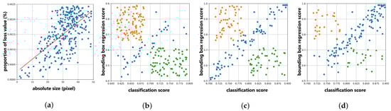
Figure 1.
Visual display of two main challenges for tiny object detection (based on VisDrone2019 [23] dataset using Faster R-CNN [24]). (a) The first image shows the relationship between absolute size of each object and the proportion of loss value obtained by each object to the total loss. Specifically, the loss values obtained by each object during an epoch of training are counted and divided by the sum of the loss values obtained by all objects, with the corresponding value on the y-axis and the red line as the trend line. (b–d) Relationships between the classification score and bounding box regression score of each sample are shown for small, medium, and large objects, respectively. The orange points represent samples with high bounding box regression scores but low classification scores, while the green points represent the opposite situation. It can be observed that the imbalance between classification score and bounding box regression score is much more severe for small objects than for large objects.
Second, most existing detectors treat the classification loss and bounding box regression loss as separate entities, which can lead to an imbalance between classification and localization tasks. Figure 1b–d illustrates the relationship between the classification score and bounding box regression score for each sample, showing that certain samples achieve high classification scores yet suffer from low-quality regression predictions, while others display accurate localization but low classification scores. This imbalance adversely affects model training and detection performance. Although methods such as YOLOv8 [25] and TOOD [26] take both the classification and regression scores into account, they primarily focus on label assignment and may overlook challenging prediction samples.
In this paper, we introduce a novel Joint Optimization Loss (JOL) designed to effectively address the aforementioned challenges in tiny object detection. First, in order to alleviate the problem of tiny objects having a much smaller proportion of the loss function during model training compared to larger objects, our JOL calculates classification and bounding box regression scores, which indicate the prediction quality of each sample. It then dynamically assigns weights to training samples based on these scores, with less accurately predicted samples receiving higher weights in order to draw the model’s attention to these challenging cases. Additionally, to alleviate the phenomenon of imbalance performance between classification and bounding box regression tasks in tiny object detection, we use the product of the classification score and bounding box regression score to evaluate the performance of each sample, which can simultaneously optimize both classification and bounding box regression tasks. Notably, our proposed method integrates seamlessly with most existing detectors and loss functions, requiring no modifications to network architectures. The main contributions of this paper are summarized as follows:
- We propose a novel Joint Optimization Loss (JOL) for tiny object detection which dynamically assigns appropriate weights to each sample in order to address the imbalance between classification and bounding box regression.
- The proposed method can be flexibly integrated with most existing detectors and loss functions without modifying the architecture of the model.
- We conducted extensive experiments on four tiny object detection datasets and one general object detection dataset to demonstrate the effectiveness of the proposed method.
The remainder of this study is organized as follows: Section 2 presents an overview of general object detection and tiny object detection algorithms along with a review of relevant work on classification and bounding box regression loss functions used in object detection tasks; Section 3 provides a comprehensive description of our proposed Joint Optimization Loss, including a visual comparison between our method and the standard loss function; Section 4 offers a detailed explanation of the datasets and implementation details used in the experiments followed by an in-depth analysis of the experimental results; Section 5 concludes the paper with a brief summary.
2. Related Work
2.1. Object Detection
Based on the absolute size of the objects, object detection tasks can be broadly categorized into general object detection and tiny object detection.
General Object Detection: Mainstream general object detectors are typically classified into two-stage and one-stage detectors based on their architecture. Two-stage detectors first generate a series of proposal regions using region proposal algorithms or networks, then classify and regress these regions to produce the final detection results. Representative two-stage detectors include R-CNN [27], Fast R-CNN [28], Faster R-CNN [24], and Mask R-CNN [29]. To achieve faster detection speeds, one-stage detectors have been developed that bypass the proposal region step and instead predict results directly for the entire image. One-stage detectors can be further classified as either anchor-based (such as RetinaNet [30], SSD [31], and YOLOv3 [32]) or anchor-free (such as FCOS [33], YOLOX [34], and CenterNet [35]) depending on whether they use anchors for bounding box regression.
Tiny Object Detection: In recent years, considerable research has been dedicated to enhancing the detection performance of small and tiny objects, particularly in high-resolution images captured from satellites and Unmanned Aerial Vehicles (UAVs), which often contain numerous densely distributed tiny objects. A common approach involves cropping the original high-resolution image into smaller patches, enlarging these patches, then detecting objects within each patch individually. Studies such as ClusDet [36], DMNet [37], CRENet [38], and CDMNet [39] have followed this method, achieving substantial improvements. Another effective approach to improve detection accuracy involves designing optimized label assignment strategies. For example, DotD [20] introduced the dot distance to replace the IoU metric for evaluating bounding box matching. NWD [21] and RFLA [22] model each bounding box as a 2D Gaussian distribution, then respectively employ the normalized Gaussian Wasserstein distance and Kullback–Leibler divergence to calculate match scores. Additionally, SimD [40] provides a novel evaluation metric that comprehensively considers both location and shape similarity. Other studies have explored effective approaches such as context modeling [41,42], attention mechanisms [43,44,45], feature fusion [46,47], and super-resolution [48,49]. Foundation models have also made significant progress, particularly in the field of remote sensing object detection. DynamicVis [50] uses a dynamic regional perception architecture and novel pretraining paradigm, achieving impressive performance on multiple remote sensing image tasks. In addition, recent reviews on tiny object detection in infrared and hyperspectral images [51,52] can also provide some inspiration thanks to their full utilization of contextual information and data characteristics.
2.2. Loss Functions for Object Detection
The loss function is a critical component in training object detectors, as it directly influences their backpropagation performance. Object detection generally involves two primary tasks: determining the locations of objects within an image, and classifying each object into its respective category.
Classification Loss: The classification loss is extensively used in tasks such as object classification, object detection, and semantic segmentation. The binary cross-entropy loss is inspired by information entropy, and is commonly applied in binary classification problems. For multiclass classification problems, using the cross-entropy loss with a softmax function allows model predictions to approximate the true category while maintaining distance from incorrect categories. Considering the issue of class imbalance, which is particularly prevalent in one-stage object detectors, Lin et al. [30] proposed the focal loss, which downweights the influence of easily classified samples and emphasizes the weights of more challenging samples. Subsequent methods inspired by focal loss include GFL [53] and VarifocalNet [54], among others.
Bounding Box Regression Loss: Accurately determining the locations of target objects is a critical aspect of object detection that is directly related to the precision of detectors. Existing bounding box regression loss functions generally fall into two categories: distance-based loss functions such as the L1, L2, and smooth L1 loss [28], and IoU-based loss functions such as the IoU [55], GIoU [56], DIoU [57], CIoU [57], and EIoU [58] loss. The L1 and L2 losses respectively compute the L1 and L2 distances between the predicted and target offsets as the bounding box regression loss value. The smooth L1 loss [28] combines their strengths by maintaining a moderate gradient when the difference is small while also preventing gradient explosion when the difference is large. Based on the recognition that bounding box coordinates are interdependent, a series of IoU-based loss functions have also been proposed. The IoU loss [55] employs the negative natural logarithm of the IoU between the predicted and target bounding boxes as the loss value. The GIoU loss [56] introduces an additional term to consider the ratio of the difference set and the minimum enclosing rectangle based on the IoU. The DIoU loss [57] addresses the limitations of constant IoU and GIoU values when a bounding box is fully enclosed within another by considering both the overlap and center point distance. The CIoU loss [57] further incorporates an aspect ratio based on the DIoU, while the EIoU loss [58] addresses aspect ratio issues by integrating the width and height of the predicted and target bounding boxes.
3. Method
3.1. Joint Optimization Loss (JOL)
The core operation when using deep learning to train a model consists of gradient updating during backpropagation, which requires a loss function. Therefore, the model will be more inclined to accurately predict objects that have a larger proportion of the loss values in the total loss function. This is one of the main reasons for the detection accuracy of tiny objects being much lower than larger ones. From this perspective, researchers have proposed label assignment strategies that are more suitable for tiny object detection by increasing the number of positive samples obtained by tiny objects and improving their proportion in the model loss function, with the goal of realizing improved detection performance.
In this paper, we adopt a more fundamental approach by directly controlling the weights of each training sample. The pipeline of our proposed Joint Optimization Loss (JOL) is illustrated in Figure 2. Prior to introducing our method, we first present a simple review of the base loss function used for object detection. In most object detectors, the total loss function consists of two parts: bounding box regression loss and classification loss. We define as the total base loss function, as shown in Equation (1):
where N denotes the number of samples in the batch and where and represent the base losses for bounding box regression and classification of the i-th sample, respectively. For example, in Faster R-CNN [24], the base loss functions for bounding box regression and classification are the L1 loss and cross-entropy loss, respectively. In addition, and are gating identifiers that distinguish between positive and negative samples. If the i-th sample is positive, then the loss function includes both classification loss and bounding box regression loss, meaning that and are equal to 1 and 0, respectively. If the i-th sample is negative, however, the loss function only includes the classification loss, meaning that and are equal to 0 and 1, respectively.
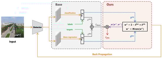
Figure 2.
Pipeline of our proposed Joint Optimization Loss (JOL). The solid lines in the flowchart represent the existing base method, while the dashed lines represent our proposed operations. The base part uses the base classification loss function and base bounding box (bbox) regression loss function to respectively calculate the base losses and in a certain batch, then adds these together to obtain the base total loss . Instead, our proposed JOL uses the classification score and bbox regression score to obtain the weight w (containing and , where is the mean weight of all positive samples) for each positive and negative sample, then multiplies the base total loss by the weight to obtain the Joint Optimization Loss . Afterwards, the model updates the parameters through backpropagation.
Our analysis and observations have identified two primary weaknesses in the existing base loss function. First, as defined in Equation (1), the current total loss function assigns equal weights to both positive and negative samples, simply combining the bounding box regression loss and classification loss to form the overall loss. This approach implicitly assumes that each sample holds equal importance for the model, which may not accurately reflect their differing contributions. Second, while several studies have proposed improved loss function calculations such as the focal loss [30] and IoU loss [55], these methods typically focus on either classification or bounding box regression in isolation. We contend that this approach may be suboptimal, as the significance of each sample should be dynamically adjusted based on its contribution to the model’s overall performance. Moreover, jointly considering both classification and bounding box regression when calculating the weights may yield better results, as accurate predictions require both precise localization and correct classification.
Based on our observations and analysis, we propose the novel Joint Optimization Loss (JOL) for tiny object detection. We define the JOL as , shown in Equation (2):
where and denote the positive and negative weights for the i-th sample, shown in Equation (3) and Equation (4), respectively; the definitions of the other parameters and symbols are as the same as in Equation (1):
where and respectively represent the bounding box regression score and classification score for the i-th sample in a certain batch. They can be calculated by any metric that can evaluate the matching degree between the prediction and target, such as the IoU for bounding box regression. The parameter controls the scale of the weights; as and usually range from zero to one, should be at least equal to one. Based on our observations, the model’s accuracy tends to stabilize when exceeds two; detailed experimental verification can be found in the second part of the ablation experiments described in Section 4.4. Therefore, we set to two for the remainder of this study. To balance the weights of positive and negative samples, we use the mean weight of all positive samples in the batch as the negative weight.
3.2. Visualization Analysis
To provide a more intuitive understanding of our method, we perform a visual analysis comparing the base loss function with our proposed Joint Optimization Loss. For demonstration purposes, we assume that the base loss functions for classification and bounding box regression are the cross-entropy loss and IoU loss [55], respectively. Additionally, we focus solely on the loss function for positive samples. Thus, the base loss function for a given sample is shown in Equation (5):
where p denotes the predicted classification score and represents the Intersection over Union (IoU) between the predicted bounding box and the ground-truth bounding box.
In our proposed Joint Optimization Loss (JOL), we use p and to represent the classification score and bounding box regression score , respectively. Accordingly, the formula for JOL is provided in Equation (6):
To visually demonstrate the similarity and difference between Equations (5) and (6), Figure 3 shows a 3D graph with p and as independent variables. It is obvious that the loss values of and are similar when the sample is well-classified and regressed; on the other hand, the value of is much larger than for the inaccurate prediction sample. This indicates that our proposed Joint Optimization Loss (JOL) can ensure that the model pays more attention to objects for which prediction is more difficult. In addition, it can be seen that only a sample with high scores in both classification and bounding box regression will obtain low loss values and be regarded as a well-predicted sample.
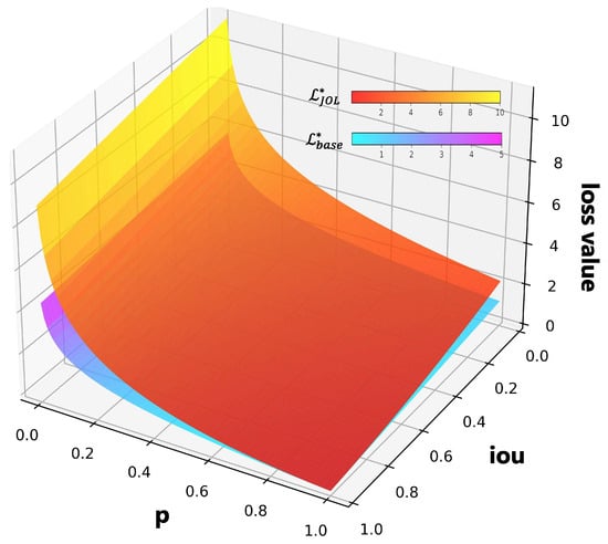
Figure 3.
Visual analysis of our proposed JOL, where represents the base loss and represents our proposed JOL. It is obvious that objects with poor classification and bounding box regression performance obtain larger loss values using our proposed JOL, enhancing the model’s attention to these objects during the training process.
4. Experiments
4.1. Datasets and Evaluation Metric
To comprehensively validate the effectiveness of our proposed method, we conducted experiments on three widely used tiny object detection datasets for remote sensing: VisDrone2019 [23], AI-TOD [59], and AI-TODv2 [60]. In addition, we validated our method on a recent tiny object detection benchmark dataset (SODA-D [13]) and a general object detection dataset (MS COCO 2017 [12]). The fundamental details of the datasets employed in the experiments are provided in Table 1.

Table 1.
Overview of datasets used in the experiments.
VisDrone2019 Dataset: The VisDrone2019 dataset [23] is a widely used benchmark for tiny object detection. It comprises 10,209 static images and 261,908 video frames extracted from 288 video clips captured by Unmanned Aerial Vehicles (UAVs) under varying scales, angles, and lighting.
AI-TOD and AI-TODv2 Datasets: The AI-TOD dataset [59] is a large-scale benchmark for tiny object detection using aerial images from remote sensing satellites. It includes 700,621 annotated objects across eight categories sourced from five public datasets, with an average object size of only 12.8 pixels. The updated AI-TODv2 dataset [60] retains the same number of images but contains additional object instances with smaller sizes and more precise annotations.
SODA-D Dataset: The SODA-D dataset [13] is a recently published benchmark for tiny object detection containing 278,433 high-quality instances collected from the MVD dataset [61] and various online sources. This dataset focuses on detecting tiny objects in diverse scenes, including city roads, highways, and rural areas.
MS COCO 2017 Dataset: The MS COCO 2017 dataset [12] is a widely used dataset for general object detection comprising over 118,000 images and 860,000 object instances across 80 categories. It serves as the official benchmark dataset for the MS COCO Detection Challenge.
Evaluation Metric: Following previous research, we chose the most commonly used COCO metric [12] to evaluate the detection performance of our method. This metric contains two basic values, namely, Precision (P) and Recall (R), respectively defined in Equations (7) and (8):
where is an abbreviation for True Positive, representing the number of positive output samples with correct predictions; is an abbreviation for False Positive, representing the number of positive output samples with incorrect predictions; and is an abbreviation for False Negative, representing the number of negative output samples with incorrect predictions. Based on Equations (7) and (8), we can obtain definitions for the Average Precision () and Mean Average Precision (), as shown in Equations (9) and (10):
where represents the area under the Precision–Recall (P-R) curve, which ranges from zero to one. The provides the average value of the for each category, with denoting the number of categories in the whole dataset.
For each detector, we report , , , , , , , and . Among these, indicates that the mean average precision under the IoU ranges from 0.5 to 0.95 at intervals of 0.05, and respectively indicate that the mean average precision under the IoU equals 0.5 or 0.75, and , , , , and represent the average precision values for objects in the very tiny, tiny, small, medium, and large size categories, respectively.
4.2. Implementation Details
We implemented all of our experiments using the common MMDetection framework [62] and PyTorch [63]. For all models, we utilized ResNet-50 [64] pretrained on ImageNet [65] as the backbone. For training, we used Stochastic Gradient Descent (SGD) as the optimizer with momentum of 0.9 and weight decay of 0.0001. The batch size and number of workers were set to 2 and 4, respectively. The initial learning rate was set to 0.005 for Faster R-CNN, Cascade R-CNN, and DetectoRS and to 0.001 for RetinaNet and FCOS.
For the VisDrone2019, SODA-D, and MS COCO 2017 datasets, in line with [13], the number of training epochs was set to 12, with the learning rate decaying by a factor of 0.1 at epochs 8 and 11. For the AI-TOD and AI-TODv2 datasets, we followed the same configuration as in [15,40] to facilitate comparison with state-of-the-art methods. We trained the models for 24 epochs, applying a learning rate decay of 0.1 at epochs 16 and 22. The RPN proposal counts for Faster R-CNN, Cascade R-CNN, and DetectoRS were all set to 3000 for both the training and testing phases. All other configurations, including the data preprocessor and anchor generator, were kept consistent with the default settings in MMDetection [62]. We conducted all of the following experiments on a computer with an Intel Xeon Gold 6326 CPU and NVIDIA RTX A6000 GPU. The versions of MMDetection, PyTorch, Python, and CUDA used are equal to 3.1.0, 2.0.1, 3.9.19, and 12.2, respectively.
4.3. Results
We conducted a series of experiments on four tiny object detection datasets (VisDrone2019, AI-TOD, AI-TODv2, and SODA-D) and a general object detection dataset (MS COCO 2017). All results reported in the tables are sourced from the corresponding papers; thus, some methods may only have results on certain datasets.
Results on VisDrone2019 Dataset: VisDrone2019 dataset is a challenging benchmark with significant scale variation, containing both tiny and general-size objects. We compared the detection performance of several commonly used object detectors before and after incorporating our proposed Joint Optimization Loss (JOL), as shown in Table 2. The first six rows display the baseline results, while the last five rows illustrate the results achieved with our method. For the one-stage RetinaNet and FCOS detectors, our method results in improvements of 6.3 and 5.8 points, respectively. For the two-stage Faster R-CNN, Cascade R-CNN, and DetectoRS detectors, our method yields improvements of 4.6, 5.3, and 3.6 points, respectively. Compared with the best-performing label assignment strategy, SimD, our method results in a 0.6-point improvement in , as shown in the sixth row of Table 2. The performance improvements are particularly notable for tiny and very tiny objects. For example, Faster R-CNN achieves detection accuracy of only 0.1 () and 6.2 () points after applying JOL, representing increases of 8.1 and 16.6, respectively, underscoring the effectiveness of our method for detecting tiny objects. Typical visual comparisons of detection performance on the VisDrone2019 dataset are shown in Figure 4, where the improvements brought about by our method are obvious.
Table 2.
Main results on VisDrone2019. All models were trained on the train set and tested on the val set. The superscript displays accuracy gains against the baseline methods.
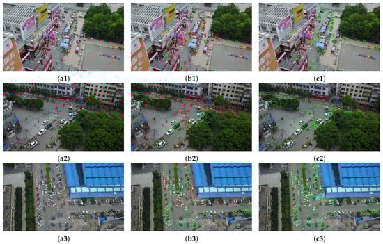

Figure 4.
Visual comparison between the baseline method and our JOL on the VisDrone2019 val set using Faster R-CNN: (a1–a6) the original images to be detected; (b1–b6) the baseline detection performance; (c1–c6) images embedded with our proposed method. The green, blue, and red rectangles respectively represent TP, FP, and FN under an IoU threshold of 0.5.
Results on AI-TOD Dataset: We conducted a comprehensive comparison of the detection performance of our method against various mainstream object detectors on the AI-TOD dataset, as shown in Table 3. The first four rows present the performance of the two-stage anchor-based detectors, rows 5–7 display the results from the one-stage anchor-based detectors, and rows 8–10 report the results for the anchor-free detectors. Notably, we also include state-of-the-art detection results from recently published research in rows 11–15. The final six rows illustrate the detection performance of our method combined with baseline and state-of-the-art detectors. Compared with base detectors, including RetinaNet, FCOS, Faster R-CNN, Cascade R-CNN, and DetectoRS, our method achieves improvements of 6.4, 5.2, 13.6, 11.7, and 12.4 points, respectively, demonstrating its adaptability across various detectors. Additionally, when combined with an existing state-of-the-art method on the AI-TOD dataset, our method yields a further improvement pf 1.7 points in terms of . Visual comparisons of the detection results and Precision–Recall (P-R) curves before and after applying our method are depicted in Figure 5 and Figure 6, respectively, highlighting the significant enhancement in performance.
Table 3.
Main results on the AI-TOD dataset. All models were trained on the trainval set and tested on the test set. The superscript displays the accuracy gains against the baseline methods.
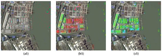
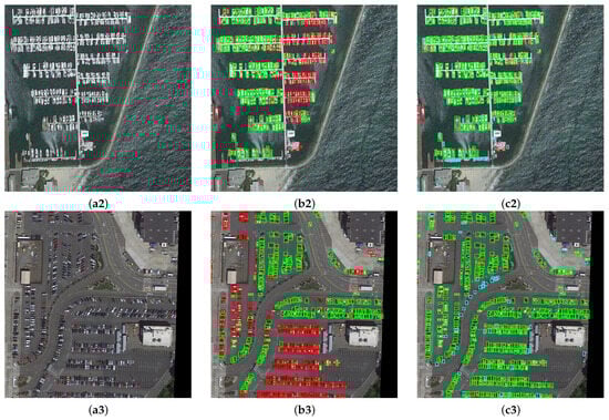
Figure 5.
Visual comparison between the base loss and JOL on the AI-TOD test set based on Faster R-CNN: (a1–a3) show the images to be detected; (b1–b3) show the original detection performance; (c1–c3) show images embedded with our proposed method. The green, blue, and red rectangles respectively represent TP, FP, and FN under an IoU threshold of 0.5.
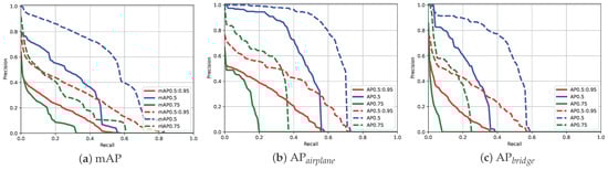
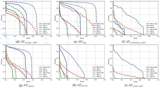
Figure 6.
Comparison of Precision–Recall (P-R) curves between baseline method and our proposed JOL on the AI-TOD dataset using Faster R-CNN: (a) shows the mean average precision across all categories, while (b–i) display the average precision for each individual category. In each plot, the solid and dashed lines represent the results from the baseline and our proposed method, respectively, with different colors indicating the results under various IoU thresholds.
Results on Other Related Datasets: The detection performance on the AI-TODv2 dataset is presented in Table 4, where we also report results from several widely used detectors of the two-stage anchor-based, one-stage anchor-based, and anchor-free varieties. Compared with the baseline RetinaNet, FCOS, Faster R-CNN, Cascade R-CNN, and DetectoRS detectors, our method achieves improvements of 7.3, 6.6, 12.2, 10.3, and 10.7 points, respectively. To further demonstrate the effectiveness of our method, we combined it with a state-of-the-art label assignment strategy for tiny object detection, as shown in the eleventh and final rows of Table 4, resulting in an increase in from 26.5 to 28.0 points. Table 5 shows detection results on the latest SODA-D tiny object detection benchmark. The first eight rows display results from existing high-performance detectors, while the last six rows present results obtained using our method. The improvements achieved by our method are substantial, especially for DetectoRS, where our method outperforms the best alternative by 1.5 points. From Figure 7, it is evident that our method successfully detects tiny objects across various categories, demonstrating its strong ability on tiny object detection tasks. To assess the adaptability of our method, we conducted an additional comparison on the MS COCO 2017 dataset, with the results shown in Table 6. Our JOL achieves an improvement of 1.1 points, indicating that it is also effective for general object detection tasks.
Table 4.
Main results on the AI-TODv2 dataset. All of the settings were as same as for the AI-TOD dataset. The superscript displays the accuracy gains against the baseline methods.
Table 5.
Main results on the SODA-D dataset. All models were trained on the train set and tested on the test set. The superscript displays the accuracy gains against the baseline methods.
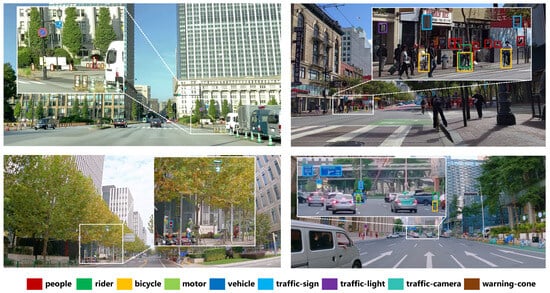
Figure 7.
Visual detection results on the test set of the SODA-D dataset using Faster R-CNN embedded with our proposed multiscale Gaussian attention mechanism. The rectangles with different colors represent different categories of objects.
Table 6.
Comparison on the MS COCO 2017 dataset. All models were based on Faster R-CNN with ResNet-50 backbone, trained on the trainval35k set, and tested on the minival set.
4.4. Ablation Study
Effectiveness of Regression and Classification Scores. Our proposed Joint Optimization Loss (JOL) incorporates both bounding box regression scores and classification scores to calculate the weight of each training sample. To further validate the effectiveness of our approach, we conducted an ablation study comparing performance when using only the classification score or only the bounding box regression score, with the results shown in Table 7. The first row displays the baseline results on AI-TOD dataset with Faster R-CNN as the detector. The second and third rows respectively show the results when using only the bounding box regression score () and only the classification score () to calculate each sample’s weight. The fourth row presents the results with the full implementation of our method. From the results in Table 7, it can be observed that there are respective improvements of 12.3 and 12.1 points when considering only the bounding box regression score and only the classification score. By incorporating both types of score simultaneously, we achieve an improvement of 13.6 points over the baseline, highlighting the effectiveness of considering both scores. This result underscores the interdependence of bounding box regression and classification, which are inseparable subtasks in object detection.
Table 7.
Ablation study evaluating the effectiveness of regression and classification scores. All of the results are based on the AI-TOD dataset using Faster R-CNN as the detector.
Performance with Different Values of . The parameter is used to control the scale of the weights. To determine the optimal value, we conducted an ablation study to evaluate the performance of models with different values of . As shown in Table 8, Faster R-CNN was used as the base detector, with all models trained on the AI-TOD trainval set and tested on the AI-TOD test set. From the results presented in Table 8, it can be observed that the model’s accuracy tends to stabilize when exceeds two. Therefore, we set equal to two.
Table 8.
Ablation study evaluating the performance of different values. All results are based on the AI-TOD dataset and use Faster R-CNN as the detector.
Analysis of Inference and Training Cost. In order to comprehensively evaluate our method, we also calculated the time and space cost of our model during inference and training, then compared the cost with that of baseline methods, including the GFLOPs and parameters of the models during inference and the speed and model size during training. As shown in Table 9, we used the RetinaNet and FOCS one-stage detectors as well as the Faster R-CNN two-stage detector as the base detectors. The models were trained on the AI-TOD trainval set and tested on the AI-TOD test set. The GFLOPs during inference were calculated for an input image size equal to 800 × 800. The conditions for calculating the speed of the training process were the same as the experimental settings mentioned above, using an NVIDIA RTX A6000 GPU for training and a batch size equal to 2.
Table 9.
Comparison of time and space cost during inference and training between our proposed JOL and baseline models. All models were based on the Faster R-CNN detector using AI-TOD trainval set for training and AI-TOD test set for testing, with the same configuration as reported in the experimental settings.
From the comparison between the baseline methods and our proposed method shown in Table 9, it is obvious that the GFLOPs, parameters during inference, and model size of our proposed JOL all remain consistent with those of the baseline methods, with only a slight decrease in the training speed of the model. Considering that our method can significantly improve the detection accuracy, our proposed JOL shows good overall performance on tiny object detection tasks.
5. Conclusions
In this paper, we have proposed the Joint Optimization Loss (JOL) for tiny object detection in remote sensing images, by which we aim to tackle the two primary challenges in the field of tiny object detection. In summary, two main factors contribute to the effectiveness and robustness of our method.
First, the proposed JOL dynamically assigns appropriate weights to each sample based on prediction performance, assigning higher weights to more challenging samples during training. This approach increases the proportion of supervisory signals for difficult-to-predict objects. Because tiny objects are generally more challenging to detect than larger ones, our method shows particularly notable accuracy improvements for tiny and very tiny objects on tiny object detection datasets.
Second, the proposed JOL comprehensively incorporates both classification and bounding box regression scores when assigning weights, enabling joint optimization of these two interdependent subtasks in object detection. This joint optimization helps to mitigate imbalance issues between classification and localization tasks. Furthermore, the JOL can be easily used with various datasets and detectors, making it highly adaptable and robust. Extensive experiments conducted across a series of widely used public datasets demonstrate the outstanding performance and robustness of our method, especially for detecting very tiny objects.
Although our method achieves significant improvements on tiny object detection datasets, its improvement on general object detection datasets is relatively limited. In the feature, we will focus on refining the proposed loss function to enhance the performance of tiny object detection while maintaining robust adaptability across varying object scales.
Author Contributions
Methodology, S.S.; Writing—original draft, S.S.; Writing—review & editing, Q.F.; Supervision, Q.F. and X.X.; Project administration, X.X. All authors have read and agreed to the published version of the manuscript.
Funding
This work is supported by the National Natural Science Foundation of China (62403483).
Data Availability Statement
Our code will be made available at: https://github.com/cszzshi/JOL, accessed on 18 April 2025.
Conflicts of Interest
The authors declare no conflicts of interest.
References
- Aneece, I.; Thenkabail, P.; Foley, D.; Oliphant, A.; Teluguntla, P. Analysis of Spaceborne Hyperspectral Sensors and Tools for Classification and Characterization of Agricultural Crops. In Proceedings of the AGU Fall Meeting Abstracts, San Francisco, CA, USA, 11–15 December 2023; Volume 2023, p. B31K-2223. [Google Scholar]
- Han, X.; Gao, J.; Yang, C.; Yuan, Y.; Wang, Q. Spotlight Text Detector: Spotlight on Candidate Regions Like a Camera. IEEE Trans. Multimed. 2024, 27, 1937–1949. [Google Scholar] [CrossRef]
- Zheng, Z.; Lv, L.; Zhang, L. Enhancing the Semi-Supervised Semantic Segmentation With Prototype-Based Supervision for Remote Sensing Images. IEEE Geosci. Remote Sens. Lett. 2024, 21, 6014705. [Google Scholar] [CrossRef]
- Huang, X.; Hu, T.; Li, J.; Wang, Q.; Benediktsson, J.A. Mapping Urban Areas in China Using Multisource Data with a Novel Ensemble SVM Method. IEEE Trans. Geosci. Remote Sens. 2018, 56, 4258–4273. [Google Scholar] [CrossRef]
- Wang, L.; Bie, W.; Li, H.; Liao, T.; Ding, X.; Wu, G.; Fei, T. Small Water Body Detection and Water Quality Variations with Changing Human Activity Intensity in Wuhan. Remote Sens. 2022, 14, 200. [Google Scholar] [CrossRef]
- Carreno-Luengo, H.; Ruf, C.S.; Gleason, S.; Russel, A. Detection of inland water bodies under dense biomass by CYGNSS. Remote Sens. Environ. 2024, 301, 113896. [Google Scholar] [CrossRef]
- Betsas, T.; Rallis, I.; Doulamis, A.; Doulamis, N.; Georgopoulos, A. Automated Detection and Categorization of River Islets Using Sentinel 2 Images. In Proceedings of the IGARSS 2024—2024 IEEE International Geoscience and Remote Sensing Symposium, Athens, Greece, 7–12 July 2024; pp. 4344–4348. [Google Scholar]
- Zong, Z.; Song, G.; Liu, Y. DETRs with Collaborative Hybrid Assignments Training. In Proceedings of the IEEE/CVF International Conference on Computer Vision (ICCV), Paris, France, 2–3 October 2023; pp. 6748–6758. [Google Scholar]
- Wang, W.; Dai, J.; Chen, Z.; Huang, Z.; Li, Z.; Zhu, X.; Hu, X.; Lu, T.; Lu, L.; Li, H.; et al. InternImage: Exploring Large-Scale Vision Foundation Models With Deformable Convolutions. In Proceedings of the IEEE/CVF Conference on Computer Vision and Pattern Recognition (CVPR), Vancouver, BC, Canada, 17–24 June 2023; pp. 14408–14419. [Google Scholar]
- Oksuz, K.; Kuzucu, S.; Joy, T.; Dokania, P.K. MoCaE: Mixture of Calibrated Experts Significantly Improves Object Detection. arXiv 2024, arXiv:2309.14976. [Google Scholar] [CrossRef]
- Fang, Y.; Wang, W.; Xie, B.; Sun, Q.; Wu, L.; Wang, X.; Huang, T.; Wang, X.; Cao, Y. EVA: Exploring the Limits of Masked Visual Representation Learning at Scale. In Proceedings of the IEEE/CVF Conference on Computer Vision and Pattern Recognition (CVPR), Vancouver, BC, Canada, 17–24 June 2023; pp. 19358–19369. [Google Scholar]
- Lin, T.Y.; Maire, M.; Belongie, S.; Hays, J.; Perona, P.; Ramanan, D.; Dollár, P.; Zitnick, C.L. Microsoft COCO: Common Objects in Context. In Proceedings of the Computer Vision—ECCV 2014, Zurich, Switzerland, 6–12 September 2014; pp. 740–755. [Google Scholar]
- Cheng, G.; Yuan, X.; Yao, X.; Yan, K.; Zeng, Q.; Xie, X.; Han, J. Towards Large-Scale Small Object Detection: Survey and Benchmarks. IEEE Trans. Pattern Anal. Mach. Intell. 2023, 45, 13467–13488. [Google Scholar] [CrossRef]
- Zhang, X.; Zhang, T.; Wang, G.; Zhu, P.; Tang, X.; Jia, X.; Jiao, L. Remote Sensing Object Detection Meets Deep Learning: A metareview of challenges and advances. IEEE Geosci. Remote Sens. Mag. 2023, 11, 8–44. [Google Scholar] [CrossRef]
- Zhou, Z.; Zhu, Y. KLDet: Detecting Tiny Objects in Remote Sensing Images via Kullback–Leibler Divergence. IEEE Trans. Geosci. Remote Sens. 2024, 62, 4703316. [Google Scholar] [CrossRef]
- Zhang, F.; Zhou, S.; Wang, Y.; Wang, X.; Hou, Y. Label Assignment Matters: A Gaussian Assignment Strategy for Tiny Object Detection. IEEE Trans. Geosci. Remote Sens. 2024, 62, 5633112. [Google Scholar] [CrossRef]
- Guo, G.; Chen, P.; Yu, X.; Han, Z.; Ye, Q.; Gao, S. Save the Tiny, Save the All: Hierarchical Activation Network for Tiny Object Detection. IEEE Trans. Circuits Syst. Video Technol. 2024, 34, 221–234. [Google Scholar] [CrossRef]
- Liu, D.; Zhang, J.; Qi, Y.; Wu, Y.; Zhang, Y. Tiny Object Detection in Remote Sensing Images Based on Object Reconstruction and Multiple Receptive Field Adaptive Feature Enhancement. IEEE Trans. Geosci. Remote Sens. 2024, 62, 5616213. [Google Scholar] [CrossRef]
- Liu, D.; Zhang, J.; Qi, Y.; Wu, Y.; Zhang, Y. A Tiny Object Detection Method Based on Explicit Semantic Guidance for Remote Sensing Images. IEEE Geosci. Remote Sens. Lett. 2024, 21, 6005405. [Google Scholar] [CrossRef]
- Xu, C.; Wang, J.; Yang, W.; Yu, L. Dot Distance for Tiny Object Detection in Aerial Images. In Proceedings of the 2021 IEEE/CVF Conference on Computer Vision and Pattern Recognition Workshops (CVPRW), Nashville, TN, USA, 19–25 June 2021; pp. 1192–1201. [Google Scholar]
- Wang, J.; Xu, C.; Yang, W.; Yu, L. A Normalized Gaussian Wasserstein Distance for Tiny Object Detection. arXiv 2022, arXiv:2110.13389. [Google Scholar] [CrossRef]
- Xu, C.; Wang, J.; Yang, W.; Yu, H.; Yu, L.; Xia, G.S. RFLA: Gaussian Receptive Field Based Label Assignment for Tiny Object Detection. In Proceedings of the Computer Vision—ECCV 2022, Tel Aviv, Israel, 23–27 October 2022; pp. 526–543. [Google Scholar]
- Zhu, P.; Wen, L.; Du, D.; Bian, X.; Fan, H.; Hu, Q.; Ling, H. Detection and Tracking Meet Drones Challenge. IEEE Trans. Pattern Anal. Mach. Intell. 2022, 44, 7380–7399. [Google Scholar] [CrossRef] [PubMed]
- Ren, S.; He, K.; Girshick, R.; Sun, J. Faster R-CNN: Towards Real-Time Object Detection with Region Proposal Networks. IEEE Trans. Pattern Anal. Mach. Intell. 2017, 39, 1137–1149. [Google Scholar] [CrossRef] [PubMed]
- Jocher, G.; Chaurasia, A.; Qiu, J. Ultralytics YOLO 2023. Available online: https://github.com/ultralytics/ultralytics (accessed on 18 April 2024).
- Feng, C.; Zhong, Y.; Gao, Y.; Scott, M.R.; Huang, W. TOOD: Task-aligned One-stage Object Detection. In Proceedings of the 2021 IEEE/CVF International Conference on Computer Vision (ICCV), Montreal, QC, Canada, 10–17 October 2021; pp. 3490–3499. [Google Scholar]
- Girshick, R.; Donahue, J.; Darrell, T.; Malik, J. Rich Feature Hierarchies for Accurate Object Detection and Semantic Segmentation. In Proceedings of the IEEE Conference on Computer Vision and Pattern Recognition (CVPR), Columbus, OH, USA, 23–28 June 2014. [Google Scholar]
- Girshick, R. Fast R-CNN. In Proceedings of the 2015 IEEE International Conference on Computer Vision (ICCV), Santiago, Chile, 7–13 December 2015; pp. 1440–1448. [Google Scholar]
- He, K.; Gkioxari, G.; Dollar, P.; Girshick, R. Mask R-CNN. In Proceedings of the IEEE International Conference on Computer Vision (ICCV), Venice, Italy, 22–29 October 2017. [Google Scholar]
- Lin, T.Y.; Goyal, P.; Girshick, R.; He, K.; Dollár, P. Focal Loss for Dense Object Detection. IEEE Trans. Pattern Anal. Mach. Intell. 2020, 42, 318–327. [Google Scholar] [CrossRef]
- Liu, W.; Anguelov, D.; Erhan, D.; Szegedy, C.; Reed, S.; Fu, C.Y.; Berg, A.C. SSD: Single Shot MultiBox Detector. In Proceedings of the Computer Vision—ECCV 2016, Amsterdam, The Netherlands, 11–14 October 2016; pp. 21–37. [Google Scholar]
- Redmon, J.; Farhadi, A. YOLOv3: An incremental improvement. arXiv 2018, arXiv:1804.02767. [Google Scholar]
- Tian, Z.; Shen, C.; Chen, H.; He, T. FCOS: Fully Convolutional One-Stage Object Detection. In Proceedings of the 2019 IEEE/CVF International Conference on Computer Vision (ICCV), Seoul, Republic of Korea, 27 October–2 November 2019; pp. 9626–9635. [Google Scholar]
- Ge, Z.; Liu, S.; Wang, F.; Li, Z.; Sun, J. YOLOX: Exceeding YOLO series in 2021. arXiv 2021, arXiv:2107.08430. [Google Scholar]
- Zhou, X.; Wang, D.; Krähenbühl, P. Objects as Points. arXiv 2019, arXiv:1904.07850. [Google Scholar] [CrossRef]
- Yang, F.; Fan, H.; Chu, P.; Blasch, E.; Ling, H. Clustered Object Detection in Aerial Images. In Proceedings of the IEEE/CVF International Conference on Computer Vision (ICCV), Seoul, Republic of Korea, 27 October–2 November 2019. [Google Scholar]
- Li, C.; Yang, T.; Zhu, S.; Chen, C.; Guan, S. Density Map Guided Object Detection in Aerial Images. In Proceedings of the IEEE/CVF Conference on Computer Vision and Pattern Recognition (CVPR) Workshops, Seattle, WA, USA, 13–19 June 2020. [Google Scholar]
- Wang, Y.; Yang, Y.; Zhao, X. Object Detection Using Clustering Algorithm Adaptive Searching Regions in Aerial Images. In Proceedings of the Computer Vision—ECCV 2020 Workshops, Glasgow, UK, 23–28 August 2020; pp. 651–664. [Google Scholar]
- Duan, C.; Wei, Z.; Zhang, C.; Qu, S.; Wang, H. Coarse-grained Density Map Guided Object Detection in Aerial Images. In Proceedings of the 2021 IEEE/CVF International Conference on Computer Vision Workshops (ICCVW), Montreal, BC, Canada, 11–17 October 2021; pp. 2789–2798. [Google Scholar]
- Shi, S.; Fang, Q.; Zhao, T.; Xu, X. Similarity Distance-Based Label Assignment for Tiny Object Detection. arXiv 2024, arXiv:2407.02394. [Google Scholar] [CrossRef]
- Liang, X.; Zhang, J.; Zhuo, L.; Li, Y.; Tian, Q. Small Object Detection in Unmanned Aerial Vehicle Images Using Feature Fusion and Scaling-Based Single Shot Detector With Spatial Context Analysis. IEEE Trans. Circuits Syst. Video Technol. 2020, 30, 1758–1770. [Google Scholar] [CrossRef]
- Hu, C.; Chen, H.; Sun, X.; Ma, F. Polarimetric SAR Ship Detection Using Context Aggregation Network Enhanced by Local and Edge Component Characteristics. Remote Sens. 2025, 17, 568. [Google Scholar] [CrossRef]
- Lu, X.; Ji, J.; Xing, Z.; Miao, Q. Attention and Feature Fusion SSD for Remote Sensing Object Detection. IEEE Trans. Instrum. Meas. 2021, 70, 5501309. [Google Scholar] [CrossRef]
- Zhang, Y.; Gao, T.; Xie, H.; Liu, H.; Ge, M.; Xu, B.; Zhu, N.; Lu, Z. Narrowband Radar Micromotion Targets Recognition Strategy Based on Graph Fusion Network Constructed by Cross-Modal Attention Mechanism. Remote Sens. 2025, 17, 641. [Google Scholar] [CrossRef]
- Liu, M.; Zhang, W.; Pan, H. Multiscale Spatial–Spectral Dense Residual Attention Fusion Network for Spectral Reconstruction from Multispectral Images. Remote Sens. 2025, 17, 456. [Google Scholar] [CrossRef]
- Hong, M.; Li, S.; Yang, Y.; Zhu, F.; Zhao, Q.; Lu, L. SSPNet: Scale Selection Pyramid Network for Tiny Person Detection From UAV Images. IEEE Geosci. Remote Sens. Lett. 2022, 19, 8018505. [Google Scholar] [CrossRef]
- Wang, Y.; Wang, X.; Qiu, S.; Chen, X.; Liu, Z.; Zhou, C.; Yao, W.; Cheng, H.; Zhang, Y.; Wang, F.; et al. Multi-Scale Hierarchical Feature Fusion for Infrared Small-Target Detection. Remote Sens. 2025, 17, 428. [Google Scholar] [CrossRef]
- Noh, J.; Bae, W.; Lee, W.; Seo, J.; Kim, G. Better to Follow, Follow to Be Better: Towards Precise Supervision of Feature Super-Resolution for Small Object Detection. In Proceedings of the 2019 IEEE/CVF International Conference on Computer Vision (ICCV), Seoul, Republic of Korea, 27 October–2 November 2019; pp. 9724–9733. [Google Scholar]
- Jiao, D.; Su, N.; Yan, Y.; Liang, Y.; Feng, S.; Zhao, C.; He, G. SymSwin: Multi-Scale-Aware Super-Resolution of Remote Sensing Images Based on Swin Transformers. Remote Sens. 2024, 16, 4734. [Google Scholar] [CrossRef]
- Chen, K.; Liu, C.; Chen, B.; Li, W.; Zou, Z.; Shi, Z. DynamicVis: An Efficient and General Visual Foundation Model for Remote Sensing Image Understanding. arXiv 2025, arXiv:2503.16426. [Google Scholar] [CrossRef]
- Chen, B.; Liu, L.; Zou, Z.; Shi, Z. Target Detection in Hyperspectral Remote Sensing Image: Current Status and Challenges. Remote Sens. 2023, 15, 3223. [Google Scholar] [CrossRef]
- Zhao, M.; Li, W.; Li, L.; Hu, J.; Ma, P.; Tao, R. Single-Frame Infrared Small-Target Detection: A survey. IEEE Geosci. Remote Sens. Mag. 2022, 10, 87–119. [Google Scholar] [CrossRef]
- Li, X.; Wang, W.; Wu, L.; Chen, S.; Hu, X.; Li, J.; Tang, J.; Yang, J. Generalized Focal Loss: Learning Qualified and Distributed Bounding Boxes for Dense Object Detection. arXiv 2020, arXiv:2006.04388. [Google Scholar] [CrossRef]
- Zhang, H.; Wang, Y.; Dayoub, F.; Sünderhauf, N. VarifocalNet: An IoU-aware Dense Object Detector. In Proceedings of the 2021 IEEE/CVF Conference on Computer Vision and Pattern Recognition (CVPR), Nashville, TN, USA, 20–25 June 2021; pp. 8510–8519. [Google Scholar]
- Yu, J.; Jiang, Y.; Wang, Z.; Cao, Z.; Huang, T. UnitBox: An Advanced Object Detection Network. In Proceedings of the 24th ACM International Conference on Multimedia, Amsterdam, The Netherlands, 15–19 October 2016; pp. 516–520. [Google Scholar]
- Rezatofighi, H.; Tsoi, N.; Gwak, J.; Sadeghian, A.; Reid, I.; Savarese, S. Generalized Intersection Over Union: A Metric and a Loss for Bounding Box Regression. In Proceedings of the 2019 IEEE/CVF Conference on Computer Vision and Pattern Recognition (CVPR), Long Beach, CA, USA, 15–20 June 2019; pp. 658–666. [Google Scholar]
- Zheng, Z.; Wang, P.; Liu, W.; Li, J.; Ye, R.; Ren, D. Distance-IoU loss: Faster and better learning for bounding box regression. In Proceedings of the AAAI 2020—34th AAAI Conference on Artificial Intelligence, New York, NY, USA, 7–12 February 2020; pp. 12993–13000. [Google Scholar]
- Zhang, Y.F.; Ren, W.; Zhang, Z.; Jia, Z.; Wang, L.; Tan, T. Focal and efficient IOU loss for accurate bounding box regression. Neurocomputing 2022, 506, 146–157. [Google Scholar] [CrossRef]
- Wang, J.; Yang, W.; Guo, H.; Zhang, R.; Xia, G.S. Tiny Object Detection in Aerial Images. In Proceedings of the 2020 25th International Conference on Pattern Recognition (ICPR), Milan, Italy, 10–15 January 2021; pp. 3791–3798. [Google Scholar]
- Xu, C.; Wang, J.; Yang, W.; Yu, H.; Yu, L.; Xia, G.S. Detecting tiny objects in aerial images: A normalized Wasserstein distance and a new benchmark. ISPRS J. Photogramm. Remote Sens. 2022, 190, 79–93. [Google Scholar] [CrossRef]
- Neuhold, G.; Ollmann, T.; Rota Bulo, S.; Kontschieder, P. The Mapillary Vistas Dataset for Semantic Understanding of Street Scenes. In Proceedings of the IEEE International Conference on Computer Vision (ICCV), Venice, Italy, 22–29 October 2017. [Google Scholar]
- Chen, K.; Wang, J.; Pang, J.; Cao, Y.; Xiong, Y.; Li, X.; Sun, S.; Feng, W.; Liu, Z.; Xu, J.; et al. MMDetection: Open MMLab Detection Toolbox and Benchmark. arXiv 2019, arXiv:1906.07155. [Google Scholar] [CrossRef]
- Paszke, A.; Gross, S.; Massa, F.; Lerer, A.; Bradbury, J.; Chanan, G.; Killeen, T.; Lin, Z.; Gimelshein, N.; Antiga, L.; et al. PyTorch: An Imperative Style, High-Performance Deep Learning Library. In Proceedings of the Advances in Neural Information Processing Systems, Vancouver, BC, Canada, 8–14 December 2019; Volume 32. [Google Scholar]
- He, K.; Zhang, X.; Ren, S.; Sun, J. Deep Residual Learning for Image Recognition. In Proceedings of the IEEE Conference on Computer Vision and Pattern Recognition (CVPR), Las Vegas, NV, USA, 27–30 June 2016. [Google Scholar]
- Krizhevsky, A.; Sutskever, I.; Hinton, G.E. ImageNet Classification with Deep Convolutional Neural Networks. In Proceedings of the Advances in Neural Information Processing Systems, Lake Tahoe, NV, USA, 3–6 December 2012; Volume 25. [Google Scholar]
- Cai, Z.; Vasconcelos, N. Cascade R-CNN: Delving Into High Quality Object Detection. In Proceedings of the 2018 IEEE/CVF Conference on Computer Vision and Pattern Recognition, Salt Lake City, UT, USA, 18–22 June 2018; pp. 6154–6162. [Google Scholar]
- Qiao, S.; Chen, L.C.; Yuille, A. DetectoRS: Detecting Objects with Recursive Feature Pyramid and Switchable Atrous Convolution. In Proceedings of the 2021 IEEE/CVF Conference on Computer Vision and Pattern Recognition (CVPR), Nashville, TN, USA, 19–25 June 2021; pp. 10208–10219. [Google Scholar]
- Vu, T.; Jang, H.; Pham, T.X.; Yoo, C. Cascade RPN: Delving into High-Quality Region Proposal Network with Adaptive Convolution. In Proceedings of the Advances in Neural Information Processing Systems, Vancouver, BC, Canada, 8–14 December 2019; Volume 32. [Google Scholar]
- Zhang, S.; Chi, C.; Yao, Y.; Lei, Z.; Li, S.Z. Bridging the Gap Between Anchor-Based and Anchor-Free Detection via Adaptive Training Sample Selection. In Proceedings of the IEEE/CVF Conference on Computer Vision and Pattern Recognition (CVPR), Seattle, WA, USA, 13–19 June 2020. [Google Scholar]
- Ge, Z.; Liu, S.; Li, Z.; Yoshie, O.; Sun, J. OTA: Optimal Transport Assignment for Object Detection. In Proceedings of the IEEE/CVF Conference on Computer Vision and Pattern Recognition (CVPR), Nashville, TN, USA, 20–25 June 2021; pp. 303–312. [Google Scholar]
- Lu, X.; Li, B.; Yue, Y.; Li, Q.; Yan, J. Grid R-CNN. In Proceedings of the IEEE/CVF Conference on Computer Vision and Pattern Recognition (CVPR), Long Beach, CA, USA, 15–20 June 2019. [Google Scholar]
- Law, H.; Deng, J. CornerNet: Detecting Objects as Paired Keypoints. Int. J. Comput. Vis. 2020, 128, 642–656. [Google Scholar] [CrossRef]
- Yang, Z.; Liu, S.; Hu, H.; Wang, L.; Lin, S. RepPoints: Point Set Representation for Object Detection. In Proceedings of the 2019 IEEE/CVF International Conference on Computer Vision (ICCV), Seoul, Republic of Korea, 27 October–2 November 2019; pp. 9656–9665. [Google Scholar]
Disclaimer/Publisher’s Note: The statements, opinions and data contained in all publications are solely those of the individual author(s) and contributor(s) and not of MDPI and/or the editor(s). MDPI and/or the editor(s) disclaim responsibility for any injury to people or property resulting from any ideas, methods, instructions or products referred to in the content. |
© 2025 by the authors. Licensee MDPI, Basel, Switzerland. This article is an open access article distributed under the terms and conditions of the Creative Commons Attribution (CC BY) license (https://creativecommons.org/licenses/by/4.0/).