Abstract
The rapid development of UAV-LiDAR and data processing capabilities is likely to enable accurate individual-tree inventories in the near future, requiring few on-ground calibration measurements. Using data collected from 20 radiata pine trials dispersed across New Zealand, the objective of this study was to determine the accuracy of high-density UAV-LiDAR for the prediction of tree diameter and volume, under a range of data calibration scenarios. Using all measurements for the calibration (a range of 335–4703 tree measurements across the 20 sites), accurate random forest models for each of the 20 sites were created from a diverse range of LiDAR metrics that characterised the horizontal and vertical structures of the canopy. Averaged across the 20 sites, predictions had a mean R2 and relative RMSE (rRMSE) of, respectively, 0.713 and 9.699% for the tree diameter and 0.746 and 19.57% for the tree volume. Reductions in the numbers of calibration trees per trial had little effect on model accuracy until only 300 trees/site were used; however, accurate, unbiased predictions were still possible using as few as 100 trees/site. More generally, applicable random forest models for both tree dimensions were constructed by collating all of the data and tested using leave-one-site-out cross-validation to determine the accuracy of the model predictions when calibration measurements were not available. The predictions using this approach were reasonable but less accurate and more biased than with the use of calibration data, with a mean R2 and rRMSE of, respectively, 0.631 and 15.12% for the tree diameter and 0.631 and 35.6% for the volume. Our research aims to facilitate the transition from a plot-based to tree-level inventory in plantation forests and contribute to the future development of a generalised model that could accurately predict tree dimensions from UAV-LiDAR, relying on minimal field measurements.
1. Introduction
Plantation forests play a critical role in meeting global wood supply demands, while providing raw materials for timber and paper industries [1,2,3]. Beyond their economic value, they contribute significantly to carbon sequestration by acting as carbon sinks, thereby helping to mitigate climate change [4,5]. Many countries rely on fast-growing species such as radiata pine (Pinus radiata D. Don.) to maintain sustainable forestry practices that deliver both economic and environmental benefits [6]. In New Zealand, radiata pine accounts for over 90% of the plantation forestry sector, and these forests are crucial for the country’s economy, export industry, and carbon offset strategies [7]. Consequently, accurate and efficient monitoring and management of these plantations are essential to maintain productivity, resilience, and long-term sustainability in a changing climate.
Effective management of plantation forests requires frequent and precise forest inventories to assess growth rates, timber yield, and overall forest health [8,9,10]. Traditional inventory methods typically rely on ground-based measurements, where tree attributes such as diameter at breast height (DBH), tree height, and stem volume are collected manually. These measurements are often obtained at the stand level, using plot averages to estimate tree attributes across a plantation. However, while these methods are widely used, they have several drawbacks, including high labour costs, time-intensive data collection, sampling bias, and limited spatial coverage [11]. The need for a more efficient, scalable, and precise inventory system has led to the increased adoption of remote sensing technologies.
Recent advancements in remote sensing technologies, particularly Light Detection and Ranging (LiDAR), have transformed forest inventory practices by enabling high-resolution, three-dimensional (3D) mapping of forest structures [12,13]. Airborne and terrestrial LiDAR systems have been extensively used to estimate tree-level attributes with high accuracy [9,14,15]. More recently, unmanned aerial vehicle (UAV)-mounted LiDAR has emerged as a cost-effective and highly flexible alternative for detailed forest inventory, especially for tree-level measurements in plantation forests [10,16,17,18]. UAV-LiDAR systems offer high spatial resolution, reduced occlusion effects, and improved cost efficiency, making them ideal for precise and repeatable forest measurements. With an increasing number of applications globally and the proliferation of consumer-grade UAV-LiDAR systems, the accessibility and affordability of this technology have significantly improved [10].
In operational inventory applications, LiDAR is most often utilised with an area-based approach (ABA) using LiDAR acquired from fixed-wing aircraft (ALS). The ABA leverages features derived from LiDAR surface models and canopy height point clouds to predict key stand attributes, using either parametric methods such as mixed-effects models or non-parametric techniques like the nearest neighbour imputation [19,20,21]. While ABA facilitates the description of the spatial variation across a stand, usually at the resolution of a plot, it does not provide information on stand density or the distributions of heights and diameters [8,22]. This approach is well suited to characterising large forests but not as cost effective as the use of UAV-derived LiDAR for small- to moderate-sized stands [23]. In contrast, the prediction of individual tree dimensions using UAV-LiDAR provides near complete censuses of stands and can provide detailed distributions of tree characteristics such as volume, height, and diameter. These outputs are especially valuable when repeat acquisitions are available, as they can be interpolated within growth simulators to determine likely volume production, grade outturn, and stand value [22].
Despite the growing adoption of UAV-LiDAR using the ABA for tree inventory, significant knowledge gaps remain around application of this methodology. The accuracy of LiDAR-based predictions using the ABA has been shown to be highly dependent on sampling density, flight parameters, and data processing techniques [11]. While the number of calibration plots can often be substantially reduced without unduly impacting the accuracy of LiDAR-derived forest estimates, changes in the predictive accuracy vary by forest type, site conditions, prediction method, and target attribute [24,25,26]. This underscores the need for more strategic sampling designs, particularly if the aim is to reduce field effort while implementing UAV-LiDAR applications.
Compared with the ABA inventory method, predictions of key individual tree metrics, such as diameter and volume, from LiDAR are less well researched. LiDAR-derived height is often used as a predictor of tree diameter because of the strong relationship and the robustness of LiDAR height measurements [27]. However, this relationship can break down in older stands, where competition effects lead to a wide range of diameters and volumes for a given height [28,29]. Thus, a number of studies have extended the set of predictor variables to include metrics describing the tree crown and the canopy structure [10,30]. In addition to ordinary least squares, commonly used parametric modelling approaches include both linear and non-linear mixed effects modelling, which are able to accommodate random variation between plots and stands [31,32]. Non-parametric methods have also been used such as random forest and k-most similar neighbour [33,34]. Compared with parametric approaches, these non-parametric methods involve fewer assumptions and can better accommodate non-linear relationships and the collinearity between predictor variables often present in LiDAR data.
Although it is critical information for developing economically feasible operational workflows, few studies have examined how individual tree prediction from LiDAR is impacted by reducing the number of measured trees. Several studies have explored how many trees are required for calibrating mixed effects models at a site different to the region over which they were fitted [32,35,36,37]. However, little research has investigated the impact of reducing tree numbers for non-parametric methods such as random forest. Two practical scenarios are especially relevant, as follows: first, how many tree measurements are needed to accurately train a random forest model at a new site; and second, whether a generalised model trained across many sites can be used to accurately predict tree dimensions at a new site without any measurements. Given that machine learning methods such as random forest require considerable data, it is likely that more calibration measurements are required than for parametric approaches.
Addressing this research gap is crucial to reducing inventory costs, improving operational efficiency and fully realizing the benefits of LiDAR technology. A better understanding of the trade-offs between field effort and model accuracy will support the transition to single-tree inventory-based workflows. Ultimately, the goal of this research is to develop a generalised model that can accurately predict tree dimensions from UAV-LiDAR using minimal field measurements. This is particularly relevant for countries like New Zealand where the forestry sector is economically important and where plantation forests have a relatively homogenous structure [7].
This study evaluates UAV-LiDAR-derived metrics for predicting tree-level diameter and volume in New Zealand radiata pine plantations across a national trial series. To achieve this goal, we used high-quality UAV-LiDAR datasets from 20 diverse sites—varying in age, stand density, and site quality—with matching field-measured tree attributes. From these data, 61 LiDAR-derived metrics were developed to characterise horizontal and vertical tree canopy structure. Using these LiDAR-derived metrics, random forest models were used to determine (i) the accuracy with which tree diameter and volume could be predicted for each site, (ii) how prediction accuracy varies with the number of measured trees in the training dataset, and (iii) using leave-one-site-out cross-validation, the extent to which tree dimensions can be predicted at an unmeasured site using a generalised model.
2. Materials and Methods
2.1. Study Site
This study used data from 20 radiata pine plantation stands distributed across New Zealand (Figure 1). These include experimental trials set up to explore methods for optimising growth rates, genetic trials, and production forest stands. The stands ranged in age from 3 to 26 years, covering all plantation forest stages, including early growth (3–6 years), mid-rotation (7–10 years), post-thinning growth (11–17 years), and late rotation (17+ years). Key attributes for all trials and a summary of the data collection dates and types of information are shown in Table 1.
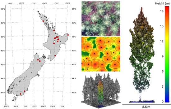
Figure 1.
The map in the left panel shows site locations (red dots) in New Zealand, while the centre panel shows an RGB image of trees from above (top) a canopy height model with delineated locations and boundaries (middle) and a side view of the point cloud with an identified tree (bottom), which is expanded upon in the right panel.

Table 1.
Site and data description. Shown is the stand age, stand area, stand density at establishment and measurement, and the year of the field and UAV-LiDAR measurements. The field height data specifies whether measurements were taken from all trees (Y), a subset of trees (Y-Subsample), or if no tree heights were measured (N). Measurements from 24 sample plots were taken at sites 18 and 19 while a complete enumeration was undertaken at all other sites. The total number of measured trees and total number of trees without malformation at each site is also shown.
2.2. Data Collection
2.2.1. Field Measurements
Tree diameter was measured at breast height (1.4 m) using a diameter tape. With the exception of sites 18 and 19, tree diameter measurements were collected for every tree across all sites. At sites 18 and 19, which were each 66 ha production forests, measuring every tree was impractical. Therefore, 24 representative sample plots were strategically established at each site for field data collection. Tree heights were primarily measured to validate remotely sensed data; therefore, they were recorded only at selected sites, either for all trees or a subsample of trees (Table 1). Tree height measurements were taken from a representative subset of trees across the height range within the site to capture size variability. Heights were measured using two methods. For smaller trials, trees were measured with a height pole with a precision of 1 cm while for taller trees (over 5 m tall), a Vertex 4 hypsometer (Haglöf, Langsele, Sweden) with a precision of 0.1 m was used.
Field inventories also recorded tree malformation, with the inventory detailing whether trees were suppressed or with multiple main leaders. This inventory also recorded trees that were dying because of disease or other physical damage, trees with a heavy lean, windthrow, including toppled and broken trees, and trees with dead crowns or those that were standing dead. The total number of trees that were measured across the 20 sites was 49,795, of which 35,201 trees, or 71%, were without malformation (Table 1).
Following the study in [38], the tree volume was determined from a tree’s basal area and height using the following equation:
where h is the tree height, ba is the basal area, and parameters a, b, and c have values of, respectively, 0.860, 0.972, and 0.340. The LiDAR-point-based metric zmax, which is defined as the maximum height, was used to estimate h, as there was a strong and unbiased relationship between zmax and h (Figure 2). The R2, RMSE, and relative RMSE for this relationship were, respectively, 0.99, 1.21 m, and 8.23%.
V = h × ba × (a × (h − 1.4)−b + c)
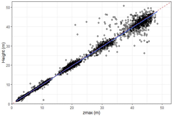
Figure 2.
Relationship between zmax and tree height, with the 1:1 line (red dashed line) and a linear line of best fit (blue line) displayed.
Table 2 shows the variation in the tree dimensions and key LiDAR metrics across all 20 sites. Height measurements included the complete range found in radiata pine within New Zealand, varying from 1.4 to 50.8 m. Both tree diameter and volume also covered the range found within commercial plantations with standard rotation length, varying from 0.5 to 72.7 cm and 0.0001 to 6.23 m3, respectively. Similarly wide ranges were found for key LiDAR metrics (Table 2).
Table 2.
Variation in the tree dimensions and key LiDAR metrics across the 20 sites.
2.2.2. LiDAR Data
UAV-LiDAR data were collected from each site using one of the following two laser scanners: a consumer-grade DJI L1 laser scanner (DJI Ltd., Shenzhen, China) mounted on a DJI M300 RTK drone (DJI Ltd., Shenzhen, China), and a scientific-grade Riegl MiniVUX-1 (MiniVUX; RIEGL Laser Measurement Systems GmbH, Horn, Austria) laser scanner mounted on a DJI M600 drone (DJI Ltd., Shenzhen, China). The flight parameters, including altitude, flying speed, and line spacing, were set based on our experience flying UAV-LiDAR across radiata pine plantation forests to obtain accurate, high-density point clouds free from motion blur. Key flight settings included an altitude of 45 m above ground level (AGL), a speed of 3–5 m/s, and line spacing between 10 and 16 m. However, for two production forest sites, the flight parameters were adjusted to a 100 m AGL, a 25 m line spacing, and a speed of 5 m/s to maintain visual line of sight (VLOS) over the canopy and ensure adequate cover and point density. Differences in sensor configurations and flight plan settings resulted in variations in the point density across the datasets collected by the two LiDAR sensors. Therefore, the point density was standardised for all captures (see Section 2.3.1) to ensure meaningful comparisons between the datasets and that differences in model accuracy were not due to variations in the point density between the two sensors. For further details on flight settings and point cloud specifications, please refer to [39].
2.3. Processing of LiDAR Data and Extraction of Predictor Variables
2.3.1. Pre-Processing of UAV-LiDAR Point Clouds
All point clouds were standardised by clipping them to stand boundaries with a 10-metre buffer zone, followed by homogenisation to ensure uniform point densities and distributions both within individual sites and across sites. This was achieved by calculating the mean and standard deviation statistics of the point clouds from a density raster with a 1 m resolution for each dataset. Each point cloud was then homogenised to a density equal to the mean plus the standard deviation using the “sample_homogenise” function within the lidR library version 4.1.2 [40] in the R programming language [41]. Each point cloud was then subjected to standard pre-processing steps, including denoising, ground point classification, and ground normalisation. These pre-processing steps were implemented using the LAStools software package version 241106 [42].
2.3.2. Digitising Stand Layouts for Creating Stem Maps
Most of the study sites did not have spatial layers representing tree locations. However, plantation forests in New Zealand are typically planted systematically with strict planting spacing. Within the 20 trials used here an establishment report was created with planting specifications (e.g., number of blocks, planting spacing, number of tree rows, number of trees per row, assigned tree labels) and a drawing of the tree layout. Using this information, we developed a semi-automated workflow to create a stand stem map for each site.
First, we digitised the forest stand establishment layout using the planting specifications and tree layouts to create georeferenced spatial layers of the established tree layout. This was then overlaid with a spatial layer of tree peaks detected from UAV-LiDAR data to identify dead, missing, and thinned tree locations. To do this, we (i) created a pit-free canopy height model (CHM) with a resolution of 25 cm using the method outlined in [43] on the ground-normalised point cloud; (ii) smoothed the CHM using a 3 × 3 pixel moving window; (iii) applied a local maxima algorithm with a fixed window size, corresponding to the initial planting spacing of the site, to detect tree peaks; and (iv) matched the detected tree peaks to the established tree locations in the spatial layer, labelling each as a tree in the stem map.
The stem maps were verified using the following three methods: visual verification of high-resolution aerial imagery, field inventory data, and ground rectification using a mobile app (Avenza, Avenza Systems, Toronto, ON, Canada). The detection of trees was assessed using accuracy, precision, recall, and F1 score which were determined as follows:
where TP are true positives, FP are false positives, and FN are false negatives. Table A1 presents a summary of the tree detection accuracy for each site. Given the homogeneous nature of the plantation settings, we achieved a high detection rate using UAV-LiDAR with an average accuracy and F1 score of, respectively, 0.93 and 0.96. The precision of 0.97 was very similar to the recall of 0.96, indicating that there were a similar number of false positives and false negatives. The majority of false negatives were trees with poor growth that did not reach the top canopy layer. False positives mainly resulted from regenerating radiata pine trees within the stand.
2.3.3. Segmentation and Extraction of UAV-LiDAR Metrics
We used a workflow to segment individual trees and extract UAV-LiDAR metrics for tree attribute modelling that included the following three key steps: tree crown delineation, point cloud segmentation, and metric extraction. This workflow was developed for plantation forests and tested across radiata pine plantations covering a range of age classes [39]. The smoothed CHM, rectified stem maps, and the normalised UAV-LiDAR point clouds were used as inputs to the workflow.
Tree crown delineation was performed by applying the marked watershed segmentation method using the “mcws” function within the ForestTools library version 1.0.2 [44] in R. The resulting crown polygons were visually assessed by overlaying them with the CHM and high-resolution aerial imagery to verify their accuracy. Any inaccurately detected polygons were rectified where possible or excluded from subsequent analysis if rectification was unfeasible.
The rectified crown polygons were then used to segment the ground-normalised point cloud into individual tree segments. A comprehensive list of individual tree metrics, representing both the vertical and horizontal structural characteristics of trees, was then calculated for each tree point cloud segment. Key metrics included the following: (i) point-based metrics, such as standard height, intensity, and canopy density, calculated using the lidR package version 4.1.2, and (ii) crown dimension metrics, such as the 2D and 3D crown surface area and volume determined using the cxhull package version 0.7.4 [45]. A comprehensive description of the metrics calculated in this study is provided in [10], and the list of metrics used is shown in Table A2.
2.4. Data Analysis
2.4.1. Overview
Random forest was used to predict the tree diameter and volume within R version 4.2.3 using the ranger package version 0.14.1, which is a fast implementation of the method [46]. Random forest was used as this modelling method is capable of handling collinear predictors and can accommodate non-linear relationships between predictors and the dependent variable [47,48]. Random forest is a tree-based method that creates a large number of decision trees with the final predictions constituting the average predictions from individual trees. The term “random” within the algorithm name is derived from the random sampling, with replacement (i.e., bootstrapping), of training observations for each learner (individual tree) within the forest and the use of a random subset of predictors at each split (node) within the tree. This approach enhances diversity among the trees, which reduces overfitting and improves generalisation to unseen data.
In the ranger package for regression, hyperparameters control the model complexity and predictive performance. The splitrule determines how nodes are split, with options including variance (minimising variance within nodes) and extratrees (randomised splits for increased diversity). The min.node.size sets the minimum number of observations in a terminal node, where smaller values lead to deeper trees and potentially better fits but may increase overfitting risk. The mtry specifies the number of predictor variables randomly considered at each split, affecting the trade-off between variance and bias, while num.trees defines the total number of trees, improving model stability as it increases but at a higher computational cost.
2.4.2. Model Fitting
We used random forest to predict the tree diameter and volume for each trial using the entire dataset with malformed trees and then limited the dataset to only trees without malformation. Using the dataset without malformation we then examined how a progressive reduction in the number of measured trees influenced model performance to understand the minimum field data requirements to obtain robust predictions. The specific steps used to undertake this analysis included examining the accuracy of the models with (i) the full number of measured trees, which was undertaken by making predictions at individual sites with the full dataset; (ii) reducing tree numbers, which involved predictions at individual sites with progressive reductions in the number of measured trees; and (iii) without any tree measurements, which involved fitting the model using leave-one-site-out cross-validation. This analysis fitted the model using data from 19 sites and withheld the 20th site as a test dataset. This process was iterated 20 times, with each site withheld once as a test dataset. This was undertaken to simulate the accuracy of the predictions at a site without any tree measurements. More details on each of the three steps are given below.
Predictions using the full dataset. Random forest was fitted to the tree diameter and volume separately for each of the 20 sites using the full dataset (malformed and non-malformed trees) and a dataset without malformed trees. The main focus of these analyses was on the dataset that included trees without malformation, as these represent the most value in the stand and provide insight into relationships between LiDAR metrics and the two stand dimensions. A recursive feature elimination (RFE) was undertaken prior to model fitting across the entire dataset, which reduced the number of variables from 61 to 29 and 30 variables, respectively, for tree diameter and volume. Using this subset of features, the dataset for each site was randomly split into a training set that included 80% of the observations, while the remaining 20% was retained as an independent test dataset. Model training used a five-fold cross-validation, and predictions were then made on the test dataset. To avoid any bias that may result from a single train/test split that included unbalanced data in either dataset, we iterated the above process 10 times using a different train/test split. The reported statistics were then averaged across all 10 iterations of the test dataset. The hyperparameter grid used for model training included the following variations: splitrule—variance or extratrees; min node size—5, 10, 15, 20, 25, 30, 35, 40; mtry—25%, 50%, 75% or 100% of the variable number in the model. All models were fitted using 500 decision trees to ensure model stability. For each site the normalised variable importance (scaled to a value of 100 for the top predictor) for the top three model predictors were determined. The most common three variables and the mean normalised variable importance scores for each site were reported.
Impact of reducing tree numbers. The methods described for the above analyses were extended to examine the impact of reducing tree number on both tree diameter and volume using the dataset without malformation. For each site the model was fitted using the maximum number of trees and then trees in the training dataset were progressively randomly reduced and the model was refitted for each reduction in tree number. The test dataset was maintained in all iterations as 20% of the total dataset size. The target numbers of trees in the training dataset were 3500, 3000, 2500, 2000, 1500, 1000, 900, 800, 700, 600, 500, 400, 300, 200, and 100. Each site by training size model was iterated 10 times, with a different train/test split to ensure stability in predictions of model performance. Given the variable number of measured trees at each site within the training dataset, which ranged from 268 to 3763 trees, many of these target training sizes were not possible as there were insufficient trees. Consequently, subsequent analyses examining the impact of tree number on model performance, only included sites with at least 1000 trees to ensure that changes were quantified in a balanced way.
Impact of no tree measurements. A leave-one-site-out cross-validation was undertaken to determine how well a generalised model across the trial series predicted tree diameter and volume on the dataset without malformation. An RFE was applied prior to model fitting using the entire set of LiDAR-based predictors, and the class variables age and stand density. This RFE reduced the predictor number from 63 to 31 and 28, respectively, for diameter and volume. Using this refined subset of predictors, the model was fitted to 19 of the 20 trials, after which predictions were then made for the withheld test trial. This process was repeated 19 times so that test datasets were available from all 20 sites. This analysis used the previously described hyperparameter grid, and all models were fitted using 500 decision trees.
2.4.3. Model Performance
Model performance for all three analyses was determined with the test dataset using the root mean square error (RMSE), coefficient of determination (R2), and mean bias error (MBE), which were calculated, respectively, as follows:
where is the observed value, is the predicted value in plot , is the average of the observed values, and is the number of plots. The relative RMSE (rRMSE) and relative MBE (rMBE) were determined, respectively, as 100 × (RMSE/) and 100 × (MBE/).
3. Results
3.1. Predictions Using Full Dataset
3.1.1. Accuracy of Predictions for Tree Diameter
Predictions of the tree diameter at individual sites using trees that were not malformed were generally quite accurate (Table 3; Figure 3). The mean rRMSE was 9.70% and ranged from 6.2 to 13.4%. The R2 averaged 0.713 with values ranging from 0.33 to 0.90 (Figure 3, Table 3). However, when the two most poorly predicted sites (R2 = 0.33, 0.36) were excluded the range narrowed considerably (R2 = 0.59–0.90). The rMBE was very low, averaging −0.04%, and it ranged from −0.49% to 0.25%, which is reflected in the plots of the predicted and actual diameters, which exhibited little apparent bias (Figure 3).
Table 3.
Statistics of the models for predicting tree diameter at each site. Shown are the RMSE, relative RMSE (rRMSE), coefficient of determination (R2), and relative mean bias error (rMBE) for trees without malformation and for all trees. The site means for all statistics for each of the four variables are displayed in the last row.
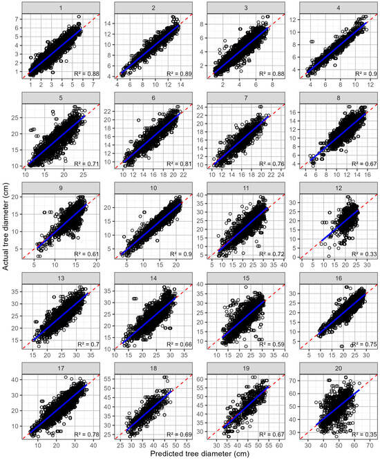
Figure 3.
Predicted values against actual tree diameters (open black circles), by site, for predictions that use all available trees that are not malformed. Shown on each plot are the 1:1 line (red dashed line) and a linear line of best fit (blue line). The site numbers are listed along the top, and the coefficient of determination for each relationship is shown in the bottom right-hand corner.
The predictions of the tree diameter using all trees, including those that were malformed, were generally accurate. The mean rRMSE was 11.12% and ranged from 7.1 to 15.5%, while the mean R2 was 0.673, ranging from 0.29 to 0.90 (Table 3). Predictions had little apparent bias using the complete dataset, as demonstrated by the relatively low rMBE, which averaged −0.30%, ranging from −1.46 to 0.404%.
3.1.2. Accuracy of Predictions for Volume
Although the predictions of the volume using trees without malformation were not as strong as for the diameter, they were still reasonably accurate (Figure 4, Table 4). The rRMSE for the predictions of the volume averaged 19.57%, ranging from 11.7 to 32.3%. The R2 averaged 0.746 and ranged from 0.42 to 0.91. The rMBE was very low, ranging from −0.556 to 0.954%, with an average of 0.112%, which reflects the lack of bias in any of the relationships (Figure 4).
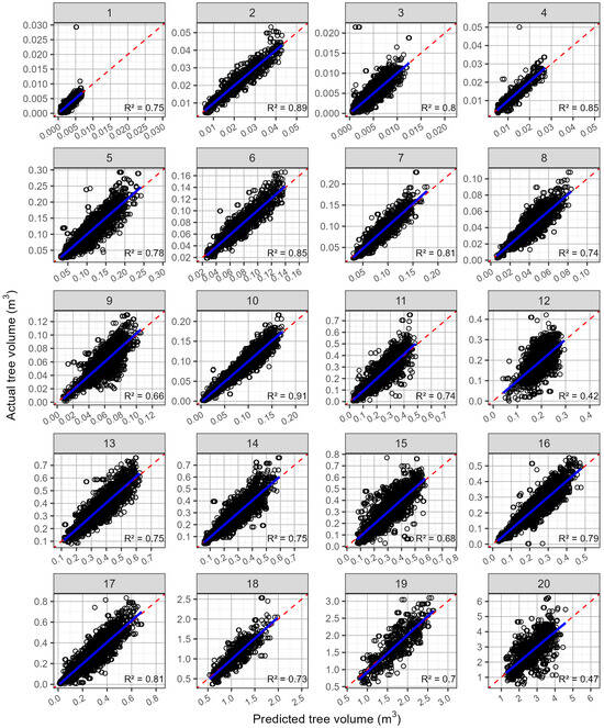
Figure 4.
Predicted values against the actual tree volume (open black circles), by site, for the predictions that used all available trees that were not malformed. Shown on each plot are the 1:1 line (red dashed line) and a linear line of best fit (blue line). The site numbers are listed along the top, and the coefficient of determination (R2) for each relationship is shown in the bottom right-hand corner.
Table 4.
Statistics of the models for predicting volume at each site. Shown are the RMSE, relative RMSE (rRMSE), coefficient of determination (R2), and relative mean bias error (rMBE) for trees without malformation and for all trees. The site means of all statistics for each of the four variables are displayed in the last row.
The accuracy of the volume predictions using all trees were similar to those described using trees that were not malformed. The rRMSE for the volume predictions averaged 21.41%, ranging from 14.3 to 30.8%. The R2 averaged 0.722 and ranged from 0.39 to 0.89 (Table 4). The predictions were relatively unbiased, and the rMBE averaged −0.30% ranging from −2.07 to 1.13%.
3.1.3. Variable Importance in Models of the Tree Diameter and Volume
For the tree diameter, the sum of the intensity of the LiDAR returns (itot) was the most influential primary predictor, ranking as the strongest predictor for 9 out of the 20 sites (Table 5). Across the sites, the itot was the most important variable more frequently within older sites, and it was the most important for 8 out of the 10 sites that were ≥9 years old. At the younger sites, the height percentiles (zq95 and zq90) were generally most important, while the area and volume of the 3D convex hull were frequently the most important in stands aged 5–9 years old. The second and third most important predictors had average normalised variable importance scores of, respectively, 77 (range 53–97) and 55 (range of 24–91). There were patterns in the predictor type with age for the second and third variables. Height percentiles were frequently important for the younger sites from ages 3 to 6 years. For the second most important predictor, the total number of points (n) was relatively common for older sites aged 9–26 years. For the third most important variable, the area or volume of the 3D convex hull was common for older sites that were ≥9 years (Table 5).
Table 5.
Variable importance for models predicting the tree diameter and volume at each site. Shown are the three most important variables for each stand dimension, with the normalised variable importance score shown after the variable in brackets. The most common predictor for each of the three variables is displayed in the last row.
For the tree volume, the most important variable was most frequently the area of the 3D convexhull, which was the most important variable for 9/20 sites (Table 5). The area of the 3D convexhull was the most important for sites up to 11 years of age, while at sites that were ≥11 years, the itot was the most important variable. The second and third most important predictors had average normalised importance scores of 78 (range 37–93) and 61 (range 32–87), respectively (Table 5). The volume of the 3D convexhull was the most common 2nd and 3rd variable, respectively, occurring at 7/20 and 6/20 trials (Table 5). Across sites, the LiDAR height metrics featured quite commonly as the first, second, or third most important variable at sites ≤ 10 years of age.
3.1.4. Variables Affecting the Model Accuracy
The strength of the model predictions at the site level, using trees that were not malformed, was correlated with several variables. The strongest determinants for tree diameter were itot, zsd, stand age, zmax, and concavehull 2D area, which all had negative relationships with R2, while ikurt had a positive relationship with R2 (Figure 5). Similarly for volume, the R2 of the model predictions was negatively related to itot, age, zsd, zmax, and also negatively related to the area and volume of the 3D convex hull. In summary, model predictions of the diameter at the site level had higher R2 values in younger stands with lower tree heights and reduced height standard deviation, with low total intensity and high values of the intensity kurtosis. These trends were similar for volume, with the highest R2 values also occurring in stands with a low volume and area for the 3D convex hull.
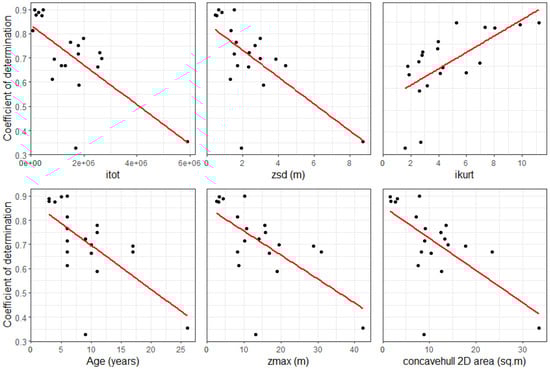
Figure 5.
Relationships between the coefficient of determination (R2) for models predicting tree diameter across the 20 sites and the six most strongly related variables (filled black circles), ranked in order from left to right and top to bottom. Also shown is a linear line of best fit to the data (red lines).
3.2. Impact of Reducing Tree Numbers
There was a steady decline in the rRMSE, with reductions in the tree number in the training dataset for diameter for all trials (Figure 6). The data were constrained to sites with at least 1000 trees so that a balanced view of the changes could be identified (red lines, Figure 6). For the predictions of the diameter, the mean rRMSE increased slowly from 10.56% for predictions made using 1000 trees to 10.89% for predictions using 300 trees. The changes were more rapid for tree numbers below this point, with the mean relative RMSE increasing to 11.08% for the model predictions using 200 trees and then 11.43% for the predictions using 100 trees. The changes in R2 largely mirrored those of the RMSE. The slight reduction in R2 was noted from 1000 trees to 300 trees, over which R2 declined from 0.702 to 0.685. The reductions in the number of trees below 300 reduced the R2 more rapidly to values of 0.676 and 0.660 for 200 and 100 trees, respectively (Figure 6).
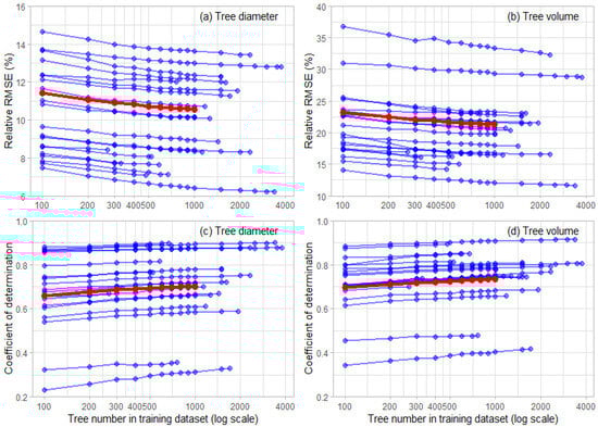
Figure 6.
Influence of the tree number in the training dataset on the relative RMSE (rRMSE) for (a) tree diameter, (b) tree volume and on coefficient of determination (R2) for (c) tree diameter and (d) tree volume. Shown are the changes for the individual sites (blue lines) and the mean changes for all trials with at least 1000 measured trees (red lines). For all models, both statistics were determined using a test dataset that was 20% of the total dataset size for each site, with the train/test split iterated 10 times to improve prediction stability.
A similar pattern was also evident with tree volume. Averaged across all sites with at least 1000 trees, there were slow increases in the rRMSE from 21.28% for the predictions made using 1000 trees to 22.04% for the predictions made using 300 trees (Figure 6). As the number of trees was further reduced, the rRMSE increased more rapidly to 22.44% and 23.19%, respectively, for the predictions made using 200 and 100 trees. Similarly, the R2 declined most markedly as the number decreased to below 300 trees. Very small reductions were noted from the predictions using 1000 trees, which had mean R2 of 0.734, to predictions using 300 trees, which had a mean R2 of 0.718. The rate of the reduction in R2 was far greater as the number declined below 300 trees to 0.710 and 0.696 for predictions using, respectively, 200 and 100 trees (Figure 6).
Little change in the rMBE was noted for either the predictions of the diameter or volume as the number of trees in the training set declined. Using the smallest training dataset of 100 trees, the range in the rMBE slightly expanded from the full dataset to −0.606 to 1.14% for the diameter and −0.885 to 2.02% for the volume. However, these values for rMBE were small, and visual examination of the predicted against the actual values for the diameter and volume for the models using 100 trees showed little apparent bias for any of the 20 sites (Figure A1 and Figure A2).
3.3. Prediction Accuracy Without Tree Measurements
The model predictions using leave-one-site-out cross-validation are shown in Table 6. For tree diameter, the mean R2 across sites was relatively high averaging 0.631, with a wide range of 0.07 to 0.87. The mean rRMSE was also relatively low at 15.12% but ranged quite widely from 9.5 to 26.0%. Averaged across all sites, the rMBE was slightly negative (−2.32%), indicating that the model underestimated the diameter on average. The values for the rMBE ranged from −23.9 to 13.0%, which also reinforces this model’s underestimation. The model underestimation was most visually apparent at sites 6, 2, and 19 (Figure 7), which is reflected by the rMBE values of, respectively, −23.90, −15.23, and −13.99% for these sites. In contrast, the diameters at trials 8, 18, and 13 were overpredicted, with rMBEs of, respectively, 13.04, 11.31, and 10.35% (Figure 7).
Table 6.
Statistics of the models for predicting the tree diameter and volume using leave-one-site-out cross-validation. Shown are the RMSE, relative RMSE (rRMSE), coefficient of determination (R2), and relative mean bias error (rMBE) for each test site.
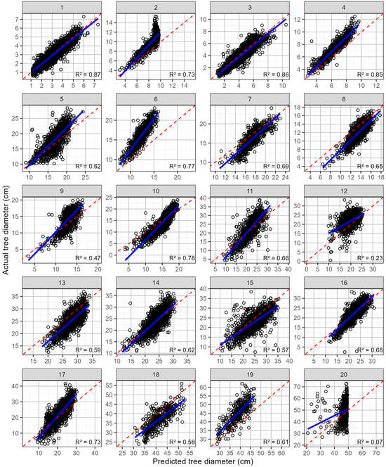
Figure 7.
Predicted against the actual tree diameter (open black circles), by site, for the leave-one-site-out cross-validation. Shown on each plot are the 1:1 line (red dashed line) and linear line of best fit (blue line). The site numbers are listed along the top, and the coefficient of determination (R2) for each relationship is shown in the bottom right-hand corner.
Similarly for the volume, the mean R2 averaged 0.631 but had a relatively wide range from 0.181 to 0.815 (Table 6). Compared with the tree diameter, the rRMSE was markedly higher, with an average value of 35.6% and a range from 19.6 to 111.6%. The predictions of the volume had a mean rMBE of 0.779% and a range of −39.5 to 55.5%, indicating that the predictions slightly overestimated the volume on average. The plots of the predicted against the actual volumes for trials 3, 8, and 18, which had rMBEs of 55.48, 30.03, and 26.90%, respectively, show marked overprediction (Figure 8). In contrast, the predictions underestimated the actual volumes at trials 6, 2, and 20, which had rMBEs of −39.45, −30.39, and −20.48, respectively (Figure 8).
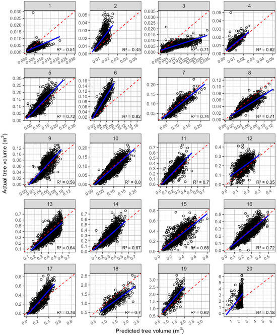
Figure 8.
The predicted against actual tree volumes (open black circles), by site, for the leave-one-site-out cross-validation. Shown on each plot are the 1:1 line (red dashed line) and linear line of best fit (blue line). The site numbers are listed along the top, and the coefficient of determination (R2) for each relationship is shown in the bottom right-hand corner.
The predictions of the diameter and volume for site 20 show limitations of not including a wide enough range in the training dataset. This 26-year-old stand, at site 20, had the largest trees of the site series, which were excluded using leave-one-site-out cross-validation when predictions were made at this site. Consequently, the predictions were constrained to the largest trees in the remainder of the site series, which were often smaller than the trees at site 20, reducing the predictive accuracy at site 20 (Table 6 and Figure 7 and Figure 8).
The R2 of the predictions of the tree diameters at the withheld test sites were most sensitive to itot, zsd, area and volume of the convexhull, and stand age, which all exhibited negative relationships with the R2. Similarly, these same variables, except for age but including zpcum1, were negatively correlated to the model’s R2 for the volume.
4. Discussion
The individual tree segmentation was highly accurate (F1 score = 0.96) with few false positives and false negatives. Detection accuracy depends on many factors, including tree species, forest complexity, point density, algorithm selection, and data quality [49,50,51]. The use of UAV-LiDAR sensors in this study, which provided very dense and accurately located point clouds, contributed to the high detection rate. High accuracy was also achieved through the systematic establishment of the layout and strict planting spacing at each site, which allowed the average planting spacing to be used as the moving window size for the detection of tree peaks. Additionally, the even-aged nature of the stands allowed for the use of a single height threshold in the tree-peak detection algorithm. For mature sites, false positives were primarily regeneration, leaning, and windthrown trees that were caught on neighbouring canopies. Within young stands, other vegetation—such as regeneration and weeds—and non-vegetative objects, such as harvest residue also contributed to these false positives. False negatives in mature stands were mainly due to suppressed trees that did not reach the canopy layer, trees with broken tops, and leaning or windthrown trees obscured by canopy closure. In young stands, significantly shorter trees that were replanted after a survival assessment and plantings in skid areas were missed because they were below the height threshold.
The height model was very accurate. Although height measurements were collected from only a subset of the full dataset, there were over 7000 observations, representing 20% of the entire dataset, which provided a robust representation of the overall height distribution. Height was predicted from the zmax, with an R2 of 0.99 and rRMSE of 8.33%, and the predictions were relatively unbiased. These results are consistent with previous research using UAV-LiDAR to predict individual tree heights, which have reported R2 values ranging from 0.65 to 0.96 and rRMSEs from 3.70 to 9.03% [52,53,54,55,56,57,58,59,60,61]. The high value of R2 found here is likely attributable to the wide range in height values in this study, as R2 tends to increase when a variable covers a wide range [62].
The predictions of the tree diameters using all of the measured trees exhibited a wide range in accuracy but were generally unbiased at all sites. The values of R2 ranged from 0.33 to 0.90, while the rRMSE ranged from 6.2 to 13.4%. This entire range was fairly similar to the combined range for the previous UAV-LiDAR predictions of the tree diameters (R2 in the range of 0.45–0.84; rRMSE in the range from 9.9 to 25.1%) [54,58,59,63,64,65,66]. The similarity in these ranges highlights the importance of site and stand conditions on model accuracy and demonstrates the wide variability covered within this study.
Compared with the predictions for the diameter, the volume estimates had slightly higher mean R2 values (0.746 vs. 0.713) but markedly lower accuracy, as indicated by the higher rRMSE values (19.57 vs. 9.70%). The higher rRMSE values for the volume predictions are consistent with previous research [65,67] and likely reflects error compounding, as the volume is determined from both the diameter and height. In contrast, R2 values were comparable between the diameter and volume, as the relative range for the volumes was wider than that for the diameters (Table 2), and R2 generally increases with a greater range [62]. There was wide variation in the accuracy of the volume predictions across the 20 sites, but the average accuracy (rRMSE = 19.57%) was consistent with previous estimates of LiDAR-predicted volumes from UAVs [59,65] and fixed-wing aircraft [67].
The predictions of the diameter and volume made for each site were most sensitive to metrics describing the tree size and structure. The area and volume of the 3D convexhull represent the spatial extent and overall size of the tree crown. As larger trees have bigger crowns, these metrics are effective proxies for tree size. The number of points (n) and the total intensity of all points (itot), respectively, measure the total number of returns and the total reflected laser energy from the tree. Both of these features depend on the foliage density, crown size, and branching structure, all of which are linked to diameter and volume [68].
The analyses showed a gradual interchange in the importance of different LiDAR-derived predictors of diameter and volume with increasing stand age. In younger stands (<6 years), which are more openly grown with minimal crown competition, LiDAR height-related metrics were typically the most important, reflecting the strong allometric relationship between tree height, diameter, and volume in early growth stages [9,69,70,71]. As stands develop further (approximately 6–11 years), simple LiDAR height metrics become less effective at capturing the variability in tree size, as crown closure occurs and trees start competing [72]. During this phase, trees begin to differentiate more in crown development, and those with broader and deeper crowns tend to accumulate a greater stem diameter and volume than similarly tall but narrower-crowned individuals. Accordingly, 3D crown shape metrics—such as the convexhull area and volume—often emerge as among the most important predictors during this stage [73]. In stands older than ca. 11 years, where crown closure, layering, and competition are more pronounced, the total intensity of LiDAR returns (itot) frequently becomes the dominant predictor. The variable itot effectively serves as a proxy for crown biomass and leaf area index (LAI) [74,75,76], since it captures canopy density and structural complexity (e.g., foliage quantity and branch structure) in the upper canopy [77]. Consequently, attributes related to leaf area and crown complexity, such as itot, play an increasingly influential role in predicting tree diameter and volume in later growth stages [77].
The variations in the R2 for diameter and volume across sites were attributable to similar variables. Generally, the model’s R2 value was highest in younger, shorter, and smaller trees, which had low values for the LiDAR’s maximum height and standard deviation of the LiDAR’s height distribution. The model’s R2 values were also high at sites with low itot and lower values for the 2D and 3D convexhull area and volume. The model accuracy was highest in stands aged ≤ 6 years, which is the age at which the optimal balance between relatively high R2 values and the lowest rRMSE occur. The mean values for the R2 and rRMSE for these stands were, respectively, 0.801 and 9.2% for the diameter and 0.808 and 19.3% for the volume. The high accuracy at this age most likely results from better laser penetration of the canopy and the homogenous stand structure, prior to significant crown competition, when height percentiles and the canopy area are still closely linked to the tree diameter and volume. When compared with the other sites, the R2 values for the nine-year-old stand at site 12 were low for both the tree diameter and stem volume. This site was heavily infested with the woody weed gorse (Ulex europaeus) and had a denser understorey, which likely impeded LiDAR penetration. The reduced canopy penetration may have affected the distribution of UAV-LiDAR points within individual tree segments, contributing to the lower R2 values in the tree attribute predictions.
The number of measured trees could be significantly reduced without a major reduction in model accuracy. Reducing the number of training trees led to only slight increases in the rRMSEs and small decreases in the R2 until the sample size dropped below 300, after which the model performance declined more noticeably. However, even with only 100 calibration trees, model accuracy was relatively similar to predictions using the complete dataset. Moreover, rMBE remained low across all sample sizes, indicating minimal bias even with reduced training data. This is an important finding because it suggests that accurate and unbiased predictions of diameter and volume can be achieved with as few as 100–300 trees, significantly reducing field data collection efforts without greatly compromising model performance. Given the high cost of tree measurement, there would be significant cost savings associated with these reductions, and this previously noted advantage of area-based LiDAR prediction [21] is also a significant advantage for tree-level estimation using LiDAR.
The model predictions for the individual sites without tree measurements were generally less accurate and far more biased. We are unaware of any comparable research that investigates the accuracy of random forest using leave-one-site-out cross-validation, and this does highlight a potential limitation of this modelling approach. The R2 was reasonable for many sites and, for instance, averaged 0.827 for predictions of the diameter in stands that were ≤5 years. However, the bias was generally quite high across the age range. This suggests that while a reasonable ranking of diameter can be obtained for young sites, which may be useful for genetic evaluation of this important trait, calibration data would generally be required to obtain an accurate estimate for inventory purposes. The limitations of having insufficient data in the training set using leave-one-site-out cross-validation were most evident for predictions made at site 20. As this was the oldest site with the largest trees, the generalised model did not robustly predict tree dimensions at this site, using the mainly smaller tree dimensions within the training set. These findings emphasise the need for comprehensive coverage of tree sizes and site conditions within the training data to support the development of robust, generalisable models.
The presented results strongly suggest that individual tree delineation and characterisation using UAV-LiDAR would be feasible for inventory purposes particularly when calibration data are available. Traditional plot-based inventory is time consuming and costly and often has high error, as it only subsamples the stand [21]. Stand inventories using LiDAR, which are typically acquired from fixed-wing aircraft, are commonly conducted using the area-based approach (ABA), which predicts key forest metrics at the plot level. However, the ABA is less cost-effective for small- to moderate-sized stands than UAV-acquired data [23] as the ABA does not predict individual tree metrics. In contrast, predictions of individual tree dimensions using UAV-LiDAR can provide an almost complete distribution of stand dimensions [8,22], which can be used within growth models to determine tree dimensions, grade outturn, and stand value at harvest [22]. A particularly useful application of the method described here by forestry companies may be in improving yield estimates for mid-rotation stands. Within New Zealand, yield tables for these stands are typically developed from silvicultural quality-control plot measurements, with growth projected forward to harvest age. The approach described in this study would overcome the variability inherent in plot sampling and provide an accurate and unbiased tree list to seed the growth model.
Further research is required to mitigate remaining impediments to widespread industry adoption of this method. Although UAV-LiDAR sensors are now a cost-effective option for inventory, data are often time-consuming to process and the conversion of raw point clouds into individual tree metrics is often a very involved multi-step process [10]. Increases in computing power and the rapid development of sophisticated algorithms and pipelines to fit models and extract useful metrics are likely to largely overcome this issue. In tandem with these developments, ground truth and LiDAR data collection should be expanded and a wider range of models should be evaluated, including deep learning approaches [78], to determine whether model generality can be improved. It would also be interesting to compare the model predictions of volume made here with those derived from photogrammetric point clouds. Further research should also evaluate whether LiDAR can be used to accurately identify malformed trees, and approaches should be developed for including these low-value trees into inventory systems, particularly at young ages before they are thinned out.
It is important to note that there are often restrictions that can hinder UAV mobilisation. These include line-of-sight constraints, regulations around UAV use, poor weather conditions, and insufficient flight endurance for the area of interest. Consequently, UAV-LiDAR acquisition will not be suitable for tree-level inventory in all situations. However, the results presented here represent a significant step forward in the establishment of the credibility of this methodology to improve inventory accuracy.
5. Conclusions
Data from a national trial series were collected, which included high-density UAV-LiDAR and ground measurements from a large number of trees in 20 radiata pine stands. Random forest models were constructed to predict the tree diameter and volume from a comprehensive set of LiDAR metrics that describe both the horizontal and vertical structures of the canopy. Using all tree measurements as calibration data, the models were, on average, accurate and unbiased, with mean R2 and rRMSE values of, respectively, 0.713 and 9.699% for the tree diameter and 0.746 and 19.57% for the tree volume. The range in the R2 values among the sites for the diameter (R2 = 0.328–0.899) and volume (R2 = 0.419–0.914) was mainly attributable to the variations in the age and LiDAR metrics describing tree size, with higher R2 values found in less structurally complex, younger stands. The reductions in the amount of calibration data had little impact on model performance, down to 300 trees/site, but even with only 100 trees/site, the models were unbiased with reasonably high accuracy for both the diameter and volume. A generalised model was fitted across all of the data and tested using leave-one-site-out cross-validation to assess the accuracy of using a model that does not include calibration data. Compared with the models that included calibration data, this model had moderate to high precision but was quite biased for both diameter (mean R2 = 0.631; rRMSE = 15.12%) and volume (mean R2 = 0.631; rRMSE = 35.6%). Through our research, we aim to support the shift from plot-based to tree-level inventories in plantation forests and contribute to the development of a generalised model capable of accurately predicting tree dimensions from UAV-LiDAR with minimal field measurements.
Author Contributions
Conceptualisation, M.S.W. and S.J.; methodology, M.S.W., S.J. and R.J.L.H.; software, S.J.; validation, S.J. and B.S.C.S.; formal analysis, M.S.W. and S.J.; investigation, S.J.; resources, R.J.L.H. and S.J.; data curation, M.S.W., B.S.C.S., S.J. and N.C.; writing—original draft preparation, M.S.W., S.J. and M.M.; writing—review and editing, M.S.W., S.J., M.M., N.C., B.S.C.S., W.Z. and M.B.; visualisation, M.S.W. and S.J.; project administration, M.S.W., R.J.L.H. and S.J.; funding acquisition, M.S.W. All authors have read and agreed to the published version of the manuscript.
Funding
This research was funded by the Ministry of Business, Innovation, and Employment (MBIE), via the programme entitled “Seeing the forest for the trees: transforming tree phenotyping for future forests” (programme grant number: C04X2101). Additional funds were provided by the Resilient Forests Research Programme, which is funded by Scion’s Strategic Science Investment Funding (SSIF), with co-funding from the Forest Growers Levy Trust.
Data Availability Statement
The data used in this study cannot be made publicly available because of privacy restrictions imposed by the forest owners and managers.
Acknowledgments
We sincerely thank the forest managers—Manulife Investment Management Forest Management NZ Ltd., Timberlands Ltd., NZ Forest Managers, Lake Taupo Forest Management, Rayonier Matariki Forests, Nelson Forests Ltd., Juken NZ Ltd., Ngati Porou Forests Ltd., Wenita Forest Products Limited, and Hautu Rangipo Whenua Limited—for granting us permission to access their sites. We are very grateful to the Radiata Pine Breeding Company (RPBC) for providing access to breeding trials to collect data, as well as field inventory data. The authors extend their sincere gratitude to various collaborators who assisted in gathering previous remote sensing and field datasets and provided clarifications regarding the data collected for various projects, including Honey Jane Estarija, Heather Flint, Stuart Fraser, John Henry, David Lane, Peter Massam, Liam Wright, David Cajes, David Pont, Damien Sellier, Kevin Park, Warren Yorston and Glen Thorlby. We also would like to thank the Accelerator Trials team at Scion—Simeon Smaill and Lorretta Garrett—and acknowledge the use of the trial series described in [79]. We also acknowledge Interpine innovation and Scion’s Tree Biometrics team for collection of the inventory and UAV-LiDAR data. We thank the two anonymous reviewers for their comments, which greatly improved the manuscript.
Conflicts of Interest
The authors declare no conflicts of interest.
Abbreviations
The following abbreviations are used in this manuscript:
| ABA | Area-based approach |
| ALS | Airborne laser scanning |
| DBH | Diameter at breast height |
| LiDAR | Light detection and ranging |
| MBE | Mean bias error |
| RMSE | Root mean square error |
| UAV | Unmanned aerial vehicle |
Appendix A
Table A1.
Statistics describing the tree detection by site. Shown are the accuracy, precision, recall, and F1 score, as well as the stand age.
Table A1.
Statistics describing the tree detection by site. Shown are the accuracy, precision, recall, and F1 score, as well as the stand age.
| Site | Age | Accuracy | Precision | Recall | F1 Score |
|---|---|---|---|---|---|
| 1 | 3 | 0.82 | 0.87 | 0.93 | 0.90 |
| 2 | 3 | 0.99 | 0.99 | 1.00 | 0.99 |
| 3 | 4 | 0.85 | 0.91 | 0.92 | 0.92 |
| 4 | 5 | 0.99 | 0.99 | 1.00 | 0.99 |
| 5 | 6 | 0.98 | 0.99 | 0.99 | 0.99 |
| 6 | 6 | 0.97 | 0.98 | 1.00 | 0.99 |
| 7 | 6 | 0.99 | 1.00 | 1.00 | 1.00 |
| 8 | 6 | 0.98 | 0.99 | 0.99 | 0.99 |
| 9 | 6 | 0.94 | 0.98 | 0.96 | 0.97 |
| 10 | 6 | 0.98 | 0.99 | 0.99 | 0.99 |
| 11 | 9 | 0.85 | 0.95 | 0.89 | 0.92 |
| 12 | 9 | 0.92 | 0.93 | 0.99 | 0.96 |
| 13 | 10 | 0.97 | 1.00 | 0.98 | 0.99 |
| 14 | 10 | 0.95 | 0.98 | 0.96 | 0.97 |
| 15 | 11 | 0.89 | 0.98 | 0.92 | 0.94 |
| 16 | 11 | 0.91 | 0.99 | 0.92 | 0.95 |
| 17 | 11 | 0.97 | 0.99 | 0.99 | 0.99 |
| 18 | 17 | 0.92 | 0.95 | 0.96 | 0.96 |
| 19 | 17 | 0.95 | 0.97 | 0.98 | 0.97 |
| 20 | 26 | 0.82 | 0.90 | 0.90 | 0.90 |
| Mean | 0.93 | 0.97 | 0.96 | 0.96 |
Table A2.
Description of the UAV-LiDAR metrics extracted from individual tree segments.
Table A2.
Description of the UAV-LiDAR metrics extracted from individual tree segments.
| Class | Description | Metric Name |
|---|---|---|
| Height | Maximum height | zmax |
| Mean height | zmean | |
| Standard deviation of the height distribution | zsd | |
| Skewness of the height distribution | zskew | |
| Kurtosis of the height distribution | zkurt | |
| Height threshold for removing understorey vegetation | zmin | |
| Percentile heights | zq5, zq10, zq15, zq20, zq25, zq30, zq35, zq40, zq45, zq50, zq55, zq60, zq65, zq70, zq75, zq80, zq85, zq90, zq95, zq99 | |
| Intensity | Sum of the intensity of the LiDAR returns | itot |
| Maximum intensity of the LiDAR returns | imax | |
| Mean intensity of the returns | imean | |
| Skewness of the intensity distribution | iskew | |
| Kurtosis of the intensity distribution | ikurt | |
| Standard deviation of the intensity distribution | isd | |
| Intensity of the ground returns | ipground | |
| Cumulative percentage of the intensity in the xth layer | ipcumzq10, ipcumzq30, ipcumzq50, ipcumzq70, ipcumzq90 | |
| Crown density | Cumulative percentage of the return in the xth layer | zpcum1, zpcum2, zpcum3, zpcum4, zpcum5, zpcum6, zpcum7, zpcum8, zpcum9 |
| Percentage of the returns above the mean height of each tree | pzabovezmean | |
| Percentage of the returns (first return–fifth return) | p1st, p2nd, p3rd, p4th, p5th | |
| Total number of points | n | |
| Crown area | 2D area of the crown concave hull | concavehull2D_area |
| 2D area of the crown convex hull | convexhull2D_area | |
| 3D volume of the individual-tree convex hull | convexhull3D_volume | |
| 3D surface area of the individual-tree convex hull | convexhull3D_area |
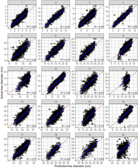
Figure A1.
The predicted values against the actual tree diameters (open black circles), by site, for the models that used a training dataset of 100 trees that were not malformed. Shown on each plot are the 1:1 line (red dashed line) and linear line of best fit (blue line).
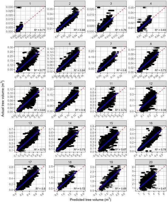
Figure A2.
The predicted values against the actual tree volumes (open black circles), by site, for the models that used a training dataset of 100 trees that were not malformed. Shown on each plot are the 1:1 line (red dashed line) and linear line of best fit (blue line).
References
- Kanninen, M. Plantation forests: Global perspectives. In Ecosystem Goods and Services from Plantation Forests; Routledge: Oxford, UK, 2010; pp. 1–15. [Google Scholar]
- Payn, T.; Carnus, J.-M.; Freer-Smith, P.; Kimberley, M.; Kollert, W.; Liu, S.; Orazio, C.; Rodriguez, L.; Silva, L.N.; Wingfield, M.J. Changes in planted forests and future global implications. For. Ecol. Manag. 2015, 352, 57–67. [Google Scholar] [CrossRef]
- Gao, T.; Zhu, J.; Deng, S.; Zheng, X.; Zhang, J.; Shang, G.; Huang, L. Timber production assessment of a plantation forest: An integrated framework with field-based inventory, multi-source remote sensing data and forest management history. Int. J. Appl. Earth Obs. Geoinf. 2016, 52, 155–165. [Google Scholar] [CrossRef]
- Myint, Y.Y.; Sasaki, N.; Datta, A.; Tsusaka, T.W. Management of plantation forests for bioenergy generation, timber production, carbon emission reductions, and removals. Clean. Environ. Syst. 2021, 2, 100029. [Google Scholar] [CrossRef]
- Watt, M.S.; Kimberley, M.O.; Steer, B.S.C.; Neumann, A. Financial comparison of afforestation using redwood and radiata pine under carbon regimes within New Zealand. Trees For. People 2023, 13, 100422. [Google Scholar] [CrossRef]
- FAO. State of the World’s Forests 2011. Food and Agricultural Organisation of the United Nations. 2011. Available online: https://www.fao.org/4/i3274e/i3274e.pdf (accessed on 25 February 2025).
- NZFOA. New Zealand Forestry Industry, Facts and Figures 2022/2023. New Zealand Plantation Forest Industry. New Zealand Forest Owners Association, Wellington. 2023. Available online: https://www.nzfoa.org.nz/images/Facts_and_Figures_2022-2023_-_WEB.pdf (accessed on 11 March 2024).
- Leite, R.V.; Amaral, C.H.d.; Pires, R.d.P.; Silva, C.A.; Soares, C.P.B.; Macedo, R.P.; Silva, A.A.L.d.; Broadbent, E.N.; Mohan, M.; Leite, H.G. Estimating stem volume in eucalyptus plantations using airborne LiDAR: A comparison of area-and individual tree-based approaches. Remote Sens. 2020, 12, 1513. [Google Scholar] [CrossRef]
- Silva, C.A.; Klauberg, C.; Hudak, A.T.; Vierling, L.A.; Jaafar, W.S.W.M.; Mohan, M.; Garcia, M.; Ferraz, A.; Cardil, A.; Saatchi, S. Predicting stem total and assortment volumes in an industrial Pinus taeda L. forest plantation using airborne laser scanning data and random forest. Forests 2017, 8, 254. [Google Scholar] [CrossRef]
- Watt, M.S.; Jayathunga, S.; Hartley, R.J.L.; Pearse, G.D.; Massam, P.D.; Cajes, D.; Steer, B.S.C.; Estarija, H.J.C. Use of a Consumer-Grade UAV Laser Scanner to Identify Trees and Estimate Key Tree Attributes across a Point Density Range. Forests 2024, 15, 899. [Google Scholar] [CrossRef]
- Silva, V.S.d.; Silva, C.A.; Mohan, M.; Cardil, A.; Rex, F.E.; Loureiro, G.H.; Almeida, D.R.A.d.; Broadbent, E.N.; Gorgens, E.B.; Dalla Corte, A.P. Combined impact of sample size and modeling approaches for predicting stem volume in eucalyptus spp. forest plantations using field and LiDAR data. Remote Sens. 2020, 12, 1438. [Google Scholar] [CrossRef]
- Silva, C.A.; Valbuena, R.; Pinagé, E.R.; Mohan, M.; de Almeida, D.R.A.; North Broadbent, E.; Jaafar, W.S.W.M.; de Almeida Papa, D.; Cardil, A.; Klauberg, C. ForestGapR: An r Package for forest gap analysis from canopy height models. Methods Ecol. Evol. 2019, 10, 1347–1356. [Google Scholar] [CrossRef]
- Silva, C.A.; Hudak, A.T.; Vierling, L.A.; Valbuena, R.; Cardil, A.; Mohan, M.; de Almeida, D.R.A.; Broadbent, E.N.; Almeyda Zambrano, A.M.; Wilkinson, B. treetop: A Shiny-based application and R package for extracting forest information from LiDAR data for ecologists and conservationists. Methods Ecol. Evol. 2022, 13, 1164–1176. [Google Scholar] [CrossRef]
- Adhikari, A.; Peduzzi, A.; Montes, C.R.; Osborne, N.; Mishra, D.R. Assessment of understory vegetation in a plantation forest of the southeastern United States using terrestrial laser scanning. Ecol. Inform. 2023, 77, 102254. [Google Scholar] [CrossRef]
- Mohan, M.; de Mendonça, B.A.F.; Silva, C.A.; Klauberg, C.; de Saboya Ribeiro, A.S.; de Araújo, E.J.G.; Monte, M.A.; Cardil, A. Optimizing individual tree detection accuracy and measuring forest uniformity in coconut (Cocos nucifera L.) plantations using airborne laser scanning. Ecol. Model. 2019, 409, 108736. [Google Scholar] [CrossRef]
- Almeida, D.; Broadbent, E.N.; Zambrano, A.M.A.; Wilkinson, B.E.; Ferreira, M.E.; Chazdon, R.; Meli, P.; Gorgens, E.B.; Silva, C.A.; Stark, S.C. Monitoring the structure of forest restoration plantations with a drone-lidar system. Int. J. Appl. Earth Obs. Geoinf. 2019, 79, 192–198. [Google Scholar] [CrossRef]
- Picos, J.; Bastos, G.; Míguez, D.; Alonso, L.; Armesto, J. Individual tree detection in a eucalyptus plantation using unmanned aerial vehicle (UAV)-LiDAR. Remote Sens. 2020, 12, 885. [Google Scholar] [CrossRef]
- Lin, Y.-C.; Liu, J.; Fei, S.; Habib, A. Leaf-off and leaf-on uav lidar surveys for single-tree inventory in forest plantations. Drones 2021, 5, 115. [Google Scholar] [CrossRef]
- Vastaranta, M.; Kankare, V.; Holopainen, M.; Yu, X.; Hyyppä, J.; Hyyppä, H. Combination of individual tree detection and area-based approach in imputation of forest variables using airborne laser data. ISPRS J. Photogramm. Remote Sens. 2012, 67, 73–79. [Google Scholar] [CrossRef]
- Næsset, E. Predicting forest stand characteristics with airborne scanning laser using a practical two-stage procedure and field data. Remote Sens. Environ. 2002, 80, 88–99. [Google Scholar] [CrossRef]
- Dash, J.P.; Marshall, H.M.; Rawley, B. Methods for estimating multivariate stand yields and errors using k-NN and aerial laser scanning. For. Int. J. For. Res. 2015, 88, 237–247. [Google Scholar] [CrossRef]
- Tompalski, P.; Coops, N.C.; White, J.C.; Goodbody, T.R.H.; Hennigar, C.R.; Wulder, M.A.; Socha, J.; Woods, M.E. Estimating changes in forest attributes and enhancing growth projections: A review of existing approaches and future directions using airborne 3D point cloud data. Curr. For. Rep. 2021, 7, 1–24. [Google Scholar] [CrossRef]
- Puliti, S.; Dash, J.P.; Watt, M.S.; Breidenbach, J.; Pearse, G.D. A comparison of UAV laser scanning, photogrammetry and airborne laser scanning for precision inventory of small-forest properties. For. Int. J. For. Res. 2020, 93, 150–162. [Google Scholar] [CrossRef]
- Li, C.; Yu, Z.; Dai, H.; Zhou, X.; Zhou, M. Effect of sample size on the estimation of forest inventory attributes using airborne LiDAR data in large-scale subtropical areas. Ann. For. Sci. 2023, 80, 40. [Google Scholar] [CrossRef]
- Maltamo, M.; Bollandsås, O.M.; Næsset, E.; Gobakken, T.; Packalén, P. Different plot selection strategies for field training data in ALS-assisted forest inventory. Forestry 2011, 84, 23–31. [Google Scholar] [CrossRef]
- Dalponte, M.; Martinez, C.; Rodeghiero, M.; Gianelle, D. The role of ground reference data collection in the prediction of stem volume with LiDAR data in mountain areas. ISPRS J. Photogramm. Remote Sens. 2011, 66, 787–797. [Google Scholar] [CrossRef]
- Popescu, S.C. Estimating biomass of individual pine trees using airborne lidar. Biomass Bioenergy 2007, 31, 646–655. [Google Scholar] [CrossRef]
- Hasenauer, H.; Burkhart, H.E.; Sterba, H. Variation in potential volume yield of loblolly pine plantations. For. Sci. 1994, 40, 162–176. [Google Scholar] [CrossRef]
- Skovsgaard, J.P.; Vanclay, J.K. Forest site productivity: A review of the evolution of dendrometric concepts for even-aged stands. For. Int. J. For. Res. 2008, 81, 13–31. [Google Scholar] [CrossRef]
- Torresan, C.; Carotenuto, F.; Chiavetta, U.; Miglietta, F.; Zaldei, A.; Gioli, B. Individual tree crown segmentation in two-layered dense mixed forests from UAV LiDAR data. Drones 2020, 4, 10. [Google Scholar] [CrossRef]
- Jääskeläinen, J.; Korhonen, L.; Kukkonen, M.; Packalen, P.; Maltamo, M. Individual Tree Inventory Based on Uncrewed Aerial Vehicle Data: How to Utilise Stand-Wise Field Measurements of Diameter for Calibration? 2024. Available online: http://urn.fi/URN:NBN:fi-fe20241220106184 (accessed on 20 January 2025).
- Korhonen, L.; Repola, J.; Karjalainen, T.; Packalen, P.; Maltamo, M. Transferability and calibration of airborne laser scanning based mixed-effects models to estimate the attributes of sawlog-sized Scots pines. Silva Fennica. 2019, 53, 10179. [Google Scholar] [CrossRef]
- Yu, X.; Hyyppä, J.; Vastaranta, M.; Holopainen, M.; Viitala, R. Predicting individual tree attributes from airborne laser point clouds based on the random forests technique. ISPRS J. Photogramm. Remote Sens. 2011, 66, 28–37. [Google Scholar] [CrossRef]
- Vauhkonen, J.; Korpela, I.; Maltamo, M.; Tokola, T. Imputation of single-tree attributes using airborne laser scanning-based height, intensity, and alpha shape metrics. Remote Sens. Environ. 2010, 114, 1263–1276. [Google Scholar] [CrossRef]
- Hao, Y.; Widagdo, F.R.A.; Liu, X.; Quan, Y.; Dong, L.; Li, F. Individual tree diameter estimation in small-scale forest inventory using UAV laser scanning. Remote Sens. 2020, 13, 24. [Google Scholar] [CrossRef]
- Fu, L.; Duan, G.; Ye, Q.; Meng, X.; Luo, P.; Sharma, R.P.; Sun, H.; Wang, G.; Liu, Q. Prediction of individual tree diameter using a nonlinear mixed-effects modeling approach and airborne LiDAR data. Remote Sens. 2020, 12, 1066. [Google Scholar] [CrossRef]
- Zhou, X.; Kutchartt, E.; Hernández, J.; Corvalán, P.; Promis, Á.; Zwanzig, M. Determination of optimal tree height models and calibration designs for Araucaria araucana and Nothofagus pumilio in mixed stands affected to different levels by anthropogenic disturbance in South-Central Chile. Ann. For. Sci. 2023, 80, 18. [Google Scholar] [CrossRef]
- Kimberley, M.O.; Beets, P.N. National volume function for estimating total stem volume of Pinus radiata stands in New Zealand. N. Z. J. For. Sci. 2007, 37, 355–371. [Google Scholar]
- Hartley, R.J.L.; Jayathunga, S.; Elleouet, J.; Steer, B.S.C.; Watt, M. UAV-Enabled Evaluation of Forestry Plantations: A Comprehensive Assessment of Laser Scanning and Photogrammetric Approaches. 2025. Available online: https://ssrn.com/abstract=5162340 (accessed on 10 March 2025).
- Roussel, J.-R.; Auty, D.; Coops, N.C.; Tompalski, P.; Goodbody, T.R.H.; Meador, A.S.; Bourdon, J.-F.; De Boissieu, F.; Achim, A. lidR: An R package for analysis of Airborne Laser Scanning (ALS) data. Remote Sens. Environ. 2020, 251, 112061. [Google Scholar] [CrossRef]
- R Core Team. R: A Language and Environment for Statistical Computing; R Foundation for Statistical Computing: Vienna, Austria, 2023; Available online: https://www.R-project.org/ (accessed on 10 January 2025).
- Isenburg, M. LAStools—Efficient LiDAR Processing Software. In (Version 190404). 2019. Available online: http://rapidlasso.com/LAStools (accessed on 1 February 2025).
- Khosravipour, A.; Skidmore, A.K.; Isenburg, M.; Wang, T.; Hussin, Y.A. Generating pit-free canopy height models from airborne lidar. Photogramm. Eng. Remote Sens. 2014, 80, 863–872. [Google Scholar] [CrossRef]
- Plowright, A.; Roussel, J. Tools for Analyzing Remote Sensing Forest Data. 2021. Available online: https://cran.r-project.org/package=ForestTools (accessed on 27 November 2024).
- Barber, C.B.; Laurent, S. The Geometry Center. 2023. Available online: https://cran.r-project.org/web/packages/cxhull/index.html (accessed on 10 January 2025).
- Wright, M.N.; Ziegler, A. ranger: A fast implementation of random forests for high dimensional data in C++ and R. arXiv 2015, arXiv:1508.04409. [Google Scholar] [CrossRef]
- Breiman, L. Random forests. Mach. Learn. 2001, 45, 5–32. [Google Scholar] [CrossRef]
- Liaw, A.; Wiener, M. Classification and regression by randomForest. R News 2002, 2, 18–22. [Google Scholar]
- Panagiotidis, D.; Abdollahnejad, A.; Surový, P.; Chiteculo, V. Determining tree height and crown diameter from high-resolution UAV imagery. Int. J. Remote Sens. 2017, 38, 2392–2410. [Google Scholar] [CrossRef]
- Cao, L.; Gao, S.; Li, P.; Yun, T.; Shen, X.; Ruan, H. Aboveground biomass estimation of individual trees in a coastal planted forest using full-waveform airborne laser scanning data. Remote Sens. 2016, 8, 729. [Google Scholar] [CrossRef]
- Larsen, M.; Eriksson, M.; Descombes, X.; Perrin, G.; Brandtberg, T.; Gougeon, F.A. Comparison of six individual tree crown detection algorithms evaluated under varying forest conditions. Int. J. Remote Sens. 2011, 32, 5827–5852. [Google Scholar] [CrossRef]
- Lisein, J.; Pierrot-Deseilligny, M.; Bonnet, S.; Lejeune, P. A photogrammetric workflow for the creation of a forest canopy height model from small unmanned aerial system imagery. Forests 2013, 4, 922–944. [Google Scholar] [CrossRef]
- Fankhauser, K.E.; Strigul, N.S.; Gatziolis, D. Augmentation of traditional forest inventory and airborne laser scanning with unmanned aerial systems and photogrammetry for forest monitoring. Remote Sens. 2018, 10, 1562. [Google Scholar] [CrossRef]
- Dalla Corte, A.P.; Rex, F.E.; Almeida, D.R.A.d.; Sanquetta, C.R.; Silva, C.A.; Moura, M.M.; Wilkinson, B.; Zambrano, A.M.A.; Cunha Neto, E.M.d.; Veras, H.F.P. Measuring individual tree diameter and height using GatorEye High-Density UAV-Lidar in an integrated crop-livestock-forest system. Remote Sens. 2020, 12, 863. [Google Scholar] [CrossRef]
- Gyawali, A.; Aalto, M.; Peuhkurinen, J.; Villikka, M.; Ranta, T. Comparison of individual tree height estimated from LiDAR and digital aerial photogrammetry in young forests. Sustainability 2022, 14, 3720. [Google Scholar] [CrossRef]
- Hu, T.; Sun, X.; Su, Y.; Guan, H.; Sun, Q.; Kelly, M.; Guo, Q. Development and performance evaluation of a very low-cost UAV-LiDAR system for forestry applications. Remote Sens. 2020, 13, 77. [Google Scholar] [CrossRef]
- Jaakkola, A.; Hyyppä, J.; Yu, X.; Kukko, A.; Kaartinen, H.; Liang, X.; Hyyppä, H.; Wang, Y. Autonomous collection of forest field reference—The outlook and a first step with UAV laser scanning. Remote Sens. 2017, 9, 785. [Google Scholar] [CrossRef]
- Zhou, X.; Ma, K.; Sun, H.; Li, C.; Wang, Y. Estimation of Forest Stand Volume in Coniferous Plantation from Individual Tree Segmentation Aspect Using UAV-LiDAR. Remote Sens. 2024, 16, 2736. [Google Scholar] [CrossRef]
- Cao, L.; Liu, H.; Fu, X.; Zhang, Z.; Shen, X.; Ruan, H. Comparison of UAV LiDAR and digital aerial photogrammetry point clouds for estimating forest structural attributes in subtropical planted forests. Forests 2019, 10, 145. [Google Scholar] [CrossRef]
- Sankey, T.; Donager, J.; McVay, J.; Sankey, J.B. UAV lidar and hyperspectral fusion for forest monitoring in the southwestern USA. Remote Sens. Environ. 2017, 195, 30–43. [Google Scholar] [CrossRef]
- Wallace, L.; Lucieer, A.; Malenovský, Z.; Turner, D.; Vopěnka, P. Assessment of forest structure using two UAV techniques: A comparison of airborne laser scanning and structure from motion (SfM) point clouds. Forests 2016, 7, 62. [Google Scholar] [CrossRef]
- Cohen, J.; Cohen, P.; West, S.G.; Aiken, L.S. Applied Multiple Regression/Correlation Analysis for the Behavioral Sciences; Routledge: Oxford, UK, 2013. [Google Scholar]
- Chisholm, R.A.; Cui, J.; Lum, S.K.Y.; Chen, B.M. UAV LiDAR for below-canopy forest surveys. J. Unmanned Veh. Syst. 2013, 1, 61–68. [Google Scholar] [CrossRef]
- Neuville, R.; Bates, J.S.; Jonard, F. Estimating forest structure from UAV-mounted LiDAR point cloud using machine learning. Remote Sens. 2021, 13, 352. [Google Scholar] [CrossRef]
- Zhang, B.; Li, X.; Du, H.; Zhou, G.; Mao, F.; Huang, Z.; Zhou, L.; Xuan, J.; Gong, Y.; Chen, C. Estimation of urban forest characteristic parameters using UAV-Lidar coupled with canopy volume. Remote Sens. 2022, 14, 6375. [Google Scholar] [CrossRef]
- Sun, Y.; Jin, X.; Pukkala, T.; Li, F. Predicting individual tree diameter of larch (Larix olgensis) from UAV-LiDAR data using six different algorithms. Remote Sens. 2022, 14, 1125. [Google Scholar] [CrossRef]
- Guerra-Hernández, J.; Cosenza, D.N.; Cardil, A.; Silva, C.A.; Botequim, B.; Soares, P.; Silva, M.; González-Ferreiro, E.; Díaz-Varela, R.A. Predicting growing stock volume of eucalyptus plantations using 3-D point clouds derived from UAV imagery and ALS data. Forests 2019, 10, 905. [Google Scholar] [CrossRef]
- Kwak, D.-A.; Cui, G.; Lee, W.-K.; Cho, H.-K.; Jeon, S.W.; Lee, S.-H. Estimating plot volume using LiDAR height and intensity distributional parameters. Int. J. Remote Sens. 2014, 35, 4601–4629. [Google Scholar] [CrossRef]
- Watt, M.S.; Kirschbaum, M.U.F. Moving beyond simple linear allometric relationships between tree height and diameter. Ecol. Model. 2011, 222, 3910–3916. [Google Scholar] [CrossRef]
- Gonzalez-Benecke, C.A.; Fernández, M.P.; Gayoso, J.; Pincheira, M.; Wightman, M.G. Using tree height, crown area and stand-level parameters to estimate tree diameter, volume, and biomass of Pinus radiata, eucalyptus globulus and eucalyptus nitens. Forests 2022, 13, 2043. [Google Scholar] [CrossRef]
- Mason, E.G. Decision-Support Systems for Establishing Radiata Pine Plantations in the Central North Island of New Zealand. Ph.D. Thesis, University of Canterbury, Christchurch, New Zealand, 1992. [Google Scholar]
- Saremi, H.; Kumar, L.; Stone, C.; Melville, G.; Turner, R. Sub-compartment variation in tree height, stem diameter and stocking in a Pinus radiata D. Don plantation examined using airborne LiDAR data. Remote Sens. 2014, 6, 7592–7609. [Google Scholar] [CrossRef]
- Popescu, S.C.; Wynne, R.H.; Nelson, R.F. Measuring individual tree crown diameter with lidar and assessing its influence on estimating forest volume and biomass. Can. J. Remote Sens. 2003, 29, 564–577. [Google Scholar] [CrossRef]
- You, H.; Wang, T.; Skidmore, A.K.; Xing, Y. Quantifying the effects of normalisation of airborne LiDAR intensity on coniferous forest leaf area index estimations. Remote Sens. 2017, 9, 163. [Google Scholar] [CrossRef]
- Luo, S.; Chen, J.M.; Wang, C.; Gonsamo, A.; Xi, X.; Lin, Y.; Qian, M.; Peng, D.; Nie, S.; Qin, H. Comparative performances of airborne LiDAR height and intensity data for leaf area index estimation. IEEE J. Sel. Top. Appl. Earth Obs. Remote Sens. 2017, 11, 300–310. [Google Scholar] [CrossRef]
- García, M.; Riaño, D.; Chuvieco, E.; Danson, F.M. Estimating biomass carbon stocks for a Mediterranean forest in central Spain using LiDAR height and intensity data. Remote Sens. Environ. 2010, 114, 816–830. [Google Scholar] [CrossRef]
- Wang, Y.; Fang, H. Estimation of LAI with the LiDAR technology: A review. Remote Sens. 2020, 12, 3457. [Google Scholar] [CrossRef]
- Windrim, L.; Bryson, M. Detection, segmentation, and model fitting of individual tree stems from airborne laser scanning of forests using deep learning. Remote Sens. 2020, 12, 1469. [Google Scholar] [CrossRef]
- Smaill, S.J.; Garrett, L.G.; Addison, S.L. Accelerator trial series in Pinus radiata stands in New Zealand: Trial establishment, site description and initial soil, forest floor and tree data. Data Brief 2023, 47, 108991. [Google Scholar] [CrossRef]
Disclaimer/Publisher’s Note: The statements, opinions and data contained in all publications are solely those of the individual author(s) and contributor(s) and not of MDPI and/or the editor(s). MDPI and/or the editor(s) disclaim responsibility for any injury to people or property resulting from any ideas, methods, instructions or products referred to in the content. |
© 2025 by the authors. Licensee MDPI, Basel, Switzerland. This article is an open access article distributed under the terms and conditions of the Creative Commons Attribution (CC BY) license (https://creativecommons.org/licenses/by/4.0/).