Analysis, Simulation, and Scanning Geometry Calibration of Palmer Scanning Units for Airborne Hyperspectral Light Detection and Ranging

Abstract

Airborne hyperspectral LiDAR (AHSL) is a technology that integrates the spectral content collected using hyperspectral imaging and the precise 3D descriptions of observed objects obtained using LiDAR (light detection and ranging). AHSL detects the spectral and three-dimensional (3D) information on an object simply using laser measurements. Nevertheless, the advantageous richness of spectral properties also introduces novel issues into the scan unit, the mechanical–optical trade-off. Specifically, the abundant spectral information requires a larger optical aperture, limiting the acceptance of the mechanic load by the scan unit at a demanding rotation speed and flight height. Via the simulation and analysis of scan models, it is exhibited that Palmer scans fit the large optical aperture required by AHSL best. Furthermore, based on the simulation of the Palmer scan model, 45.23% is explored as the optimized ratio of overlap (ROP) for minimizing the diversity of the point density, with a reduction in the coefficient of variation (CV) from 0.47 to 0.19. The other issue is that it is intricate to calibrate the scanning geometry using outside devices due to the complex optical path. A self-calibration strategy is proposed for tackling this problem, which integrates indoor laser vector retrieval and airborne orientation correction. The strategy is composed of the following three improvements: (1) A self-determined laser vector retrieval strategy that utilizes the self-ranging feature of AHSL itself is proposed for retrieving the initial scanning laser vectors with a precision of 0.874 mrad. (2) A linear residual estimated interpolation method (LREI) is proposed for enhancing the precision of the interpolation, reducing the RMSE from 1.517 mrad to 0.977 mrad. Compared to the linear interpolation method, LREI maintains the geometric features of Palmer scanning traces. (3) A least-deviated flatness restricted optimization (LDFO) algorithm is used to calibrate the angle offset in aerial scanning point cloud data, which reduces the standard deviation in the flatness of the scanning plane from 1.389 m to 0.241 m and reduces the distortion of the scanning strip. This study provides a practical scanning method and a corresponding calibration strategy for AHSL.

1. Introduction

Airborne laser scanning (ASL), specifically airborne light detection and ranging (LiDAR), has become one of the prime remote sensing technologies for acquiring three-dimensional (3D) information on the Earth’s surface [1]. In terms of previous technical methods, monochromatic LiDAR can acquire high-resolution 3D information on objects on the ground [2,3]. Constrained by its single-wavelength emission and detection mechanisms, it cannot further express multispectral physical information on ground objects [4]. Meanwhile, passive spectral imaging methods can detect ground objects with a high spectral resolution and retrieve rich physical information but cannot detect three-dimensional information.

Compared with the use of the data source only, a combination of multispectral images and regular LiDAR data could achieve better results in the classification and detection of forest diseases [5,6]. To address this challenge, previous studies have focused on the fusion of heterogeneous sensing data to couple 3D and spectral information from LiDAR and hyperspectral cameras, respectively [7]. However, this method faces challenges in its “point” and “facet” fusion mechanisms and difficulties in reducing matching errors. Previous airborne multispectral LiDAR systems, such as the dual-wavelength Leica Chiroptera system [8] and the Optech Titan [9], have been developed for mapping urban areas. Such airborne multispectral LiDAR systems emit multiple laser beams in different wavelengths to collect more spectral information. Although every beam produces an independent laser signature in the same pulse cycle, it cannot provide the exact matched spectral information for each illuminated point [10]. This multispectral LiDAR mechanism requires resampling algorithms for the laser foot points to reconstruct the spectral information in each scan scene [11]. Nevertheless, an unmatched monochromatic laser beam increases the complexity of the data processing and limits its further application.

In recent years, a multispectral/hyperspectral LiDAR detection mechanism was proposed for avoiding the above problems caused by the fusion of multiple-source data [12] which expanded the spectral width of the emission end significantly using a supercontinuum laser as the light source. Then, it explicitly increased the number of receiving wavelengths by independently detecting the channels. This mechanism uses a single laser foot point to simultaneously acquire geometric information and multispectral reflectance spectrum information from the scan scene [13]. Also, [14,15,16] proposed a design for an optical receiving unit for AHSL. Meanwhile, [17,18] indicate that AHSL requires an optical aperture of more than 170 mm to successfully complete a normal aerial survey mission at a height of more than 500 m. The large optical aperture in AHSL introduces novel issues and difficulties into the scanning method and the scanning geometry calibration.

On the one hand, it is worth noting that the useful richness of the spectral properties detected using AHSL also introduces a novel issue into the design of the scanning unit, the mechanical–optical trade-off. Specifically, a larger optical aperture is required to collect more back-reflected energy from the abundant spectral information for an effective radiometric response from each detector [18]. A regular scanning unit for ASL includes an oscillating mirror, a rotating polygon, and the Palmer scan method [19]. In [20], it was found that the scanning speed is a critical parameter for reducing deviations in the point density and enhancing the quality of the scanned images. Nevertheless, the scanning speed is limited by the mechanic load of the motor. In [21], the original design of the oscillating mirror was modified to reduce variations in the scanning density. The load acceptance of the usual scanning mechanisms needs to be analyzed and optimized. Furthermore, the scan model can be determined using a series of parameters, including the motor control load, the quality of the scanning mirror, and optimization of the scan strip [22]. In this work, the theoretical scanning geometry of these methods is introduced first, and then models with the above parameters are simulated and quantitatively analyzed to illustrate that Palmer scans are a proper method for AHSL. Furthermore, the optimized ratio of overlap (ROP) in the scan trace is determined to reduce the density of the AHSL flight strip.

On the other hand, calibration of the scanning geometry requires the inner orientation elements of the laser vectors to be determined in all scanning directions. Previous research has assumed that the scanning trace coincides with the theoretic trace and has ignored the offset in the initial scanning angle implemented by the optical encoder. This typical calibration set works with the assumption that the optical path for LiDAR is finely designed and is not adjustable in aerial survey missions. However, the optical path in AHSL is more complex than that in normal monochromatic LiDAR, introducing a series of reflectors and adjustments according to the demanding height of aerial surveys [18]. Thus, a method is needed to measure the primary inner orientation elements directly.

We propose a novel strategy specialized for AHSL to tackle these issues. This strategy provides and calibrates the scanning geometry for AHSL using the following three key steps.

• An indoor self-orientation element measurement method is proposed. This method utilizes the indoor self-ranging feature of AHSL, owing to its sizable optical aperture, which obtains the distance and position of the laser points
• The linear residual estimated interpolation (LREI) method is used to obtain the whole scanning trace (with the orientation elements at all scanning angles recorded), and integrating the linear residual estimation interpolation method with a simulation of the Palmer scan model is proposed to improve the precision and maintain the features of the ellipse-like pattern produced by the Palmer scan.
• Least-deviated flatness optimization (LDFO) is proposed for iteratively calibrating the offset of the scanning angle. The effect of the angle offset on the geometry of the scanning trace is explored through simulation of the Palmer scan model. LDFO integrates a point cloud of the horizontal ground plane as the data input accounting for the restriction of the LREI method to iteratively optimize the calibration.

2. Materials

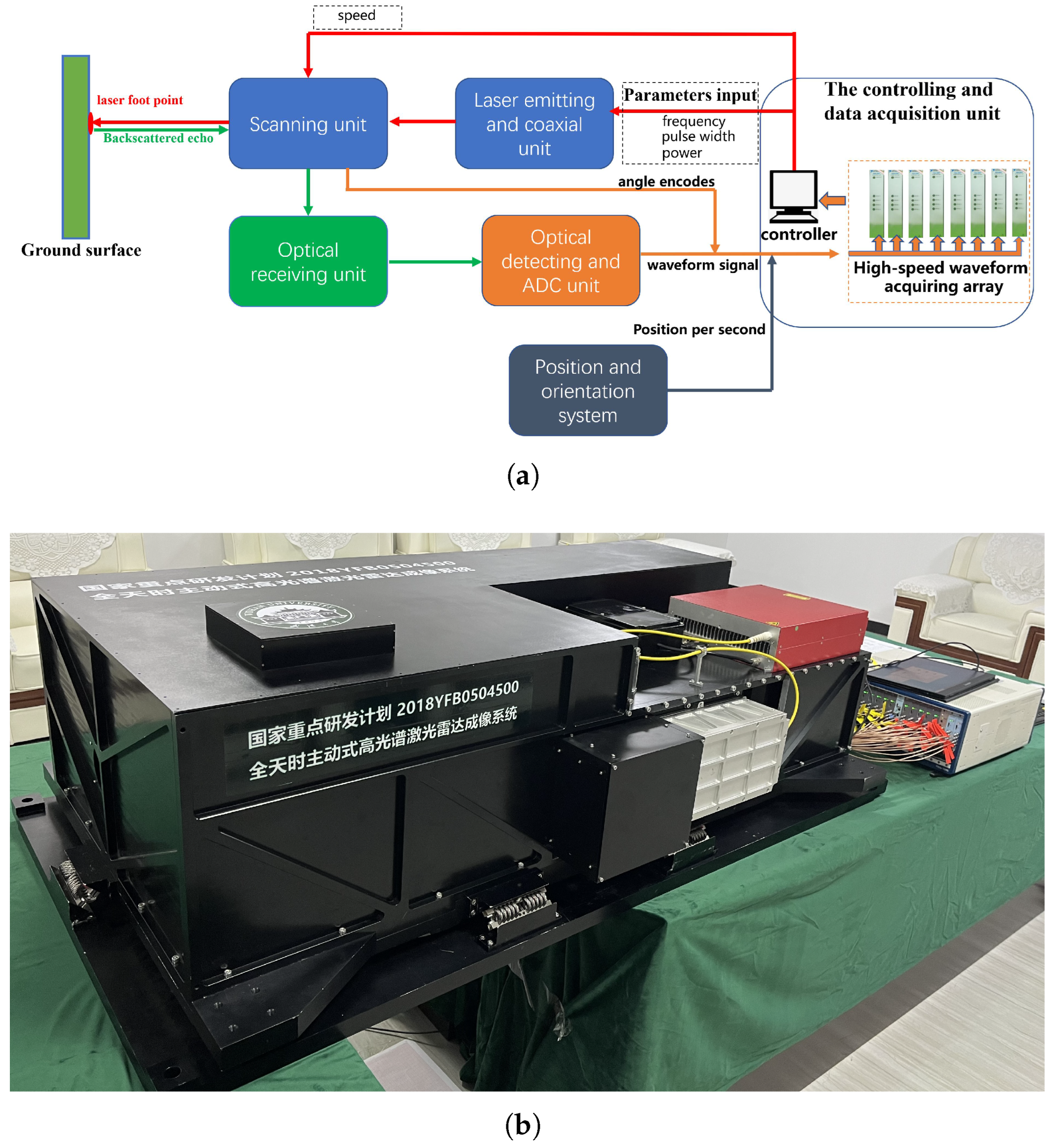
2.1. The Airborne Hyperspectral LiDAR System

The structure of the whole AHSL system is exhibited in the following, Figure 1. As shown in Figure 1, the AHSL system is composed of six units: a laser emission and coaxial unit, a scanning unit, an optical receiving unit, an optical detection and Analog–Digital Converter (ADC) unit, a position and orientation system (POS) unit, and a system control and data acquisition unit. The POS unit comprises an AV 510 type controller (Trimble, Applanix company, Richmond Hill, ON, Canada) and POSPAC 8.0 software (Trimble, Applanix company) for generating the flight path data, resulting in a flight path that is the epitome of accuracy for generating the airborne scanning point cloud. This system uses a supercontinuum laser light source with a spectrum coverage ranging from 400 nm to 900 nm and a 0.3-mrad convergence angle. Laser pulses at different wavelengths are coaxially emitted. The optical receiving unit utilizes a 170 mm diameter optical aperture to ensure efficiency in capturing the echo light pulse. The large optical aperture allows for the collection and capture of back-reflected echoes in abundant wavelengths and also ensures indoor self-ranging and comprehensive data acquisition. The detection and ADC unit comprises a 56-channel independent photomultiplier tube (PMT) array for detection. The signal of the PMT array is digitized using a high-speed waveform acquisition array. To ensure the synchronization of multi-source data, a synchronizing card is used to frame the waveform signal, the code of the scanning angle, and the pulse per second (PPS) signal simultaneously generated by the POS unit. This process aligns the data from different units, allowing the AHSL system to generate a comprehensive and accurate point cloud with aerial laser scan measurements.

2.2. An Analysis of the Scanning Methods for AHSL

This section simulates and evaluates the performance of three scanning methods in balancing the mechanical–optical trade-off issue. Then, an appropriate scanning method for AHSL is determined.

2.2.1. The Typical Scanning Methods for ASL

The usual scanning mechanisms employed in aerial surveying LiDAR are oscillating mirrors and rotating mirrors. Models of these scan methods are shown in the following, Figure 2.

As depicted in Figure 2a, the oscillating mirror produces a zigzag line with forward and backward scanning. During each scan, the mirror rotates around the center point with a given field of view (FOV). This scanning method contains four accelerating and moderating processes in the law of sines. The angular speed $\omega$ has a direct ratio to the motor current C. The principle of this scan is shown in Figure 2a. According to the law of specular reflection, the angular speed varies with a high-frequency change in the scanning angle x by $C\left(x\right)=C_{max}sin\left({\displaystyle \frac{2\pi }{FOV}}x\right)$, conducting the high-frequency components in the motor control hardware.

The rotating polygon produces parallel scanning lines. Points along a line are scanned at equal angle steps. Unlike the oscillating mirror method, the angular speed of the rotating polygon is usually stable, effectively reducing the high-frequency component of the electrical control unit. However, the spatial size of the rotating polygon is significantly larger than that in the oscillating mirror method. Its spatial size can be expressed by $V_{rm}={\displaystyle \frac{4}{3}}{D}^3$. V represents the spatial size of the scanning unit, and D is the aperture of the optical receiving unit. Compared to $\sqrt{2}T{h}_{osci}.D^2$ ($T{h}_{osci}$: the thickness of the oscillating mirror) for the oscillating mirror, the spatial size of the rotating polygon is larger, introducing a heavier load on the electric motor.

Apart from the infeasible loading on the mechanics, its scanning geometry also presents an inevitable disadvantage in terms of optical issues. Due to the limited FOV (30° in our implementation of AHSL), there is a significant loss in the effective echo when the scanning angle is more extensive than the FOV. The density of points is also significantly reduced since the total scanning points $P\left(t\right)$ are determined by $P\left(t\right)=f.t$, where t is the scanning time(s) and f(Hz) is the repetition rate of the laser pulse. Then, the loss of scanning points ($LSP$) can be determined using Equation (1).

$$LSP=1-{\displaystyle \frac{2}{\pi }}FOV$$

(1)

Furthermore, AHSL implements the required aerial surveys at a flight height greater than 300 m. Considering that the convergence angle of the laser beam is 0.3 mrad, the diameter of the laser foot point at the lowest flight height is greater than 90 mm. As shown in Figure 2, this is significantly larger than the diameter of the scanning mirror. This outcome results in an “edge effect” phenomenon. Specifically, when the field of the laser foot point collected by the mirror is over the edge of the reflector, the echo will not be fully collected, creating radiometric distortion.

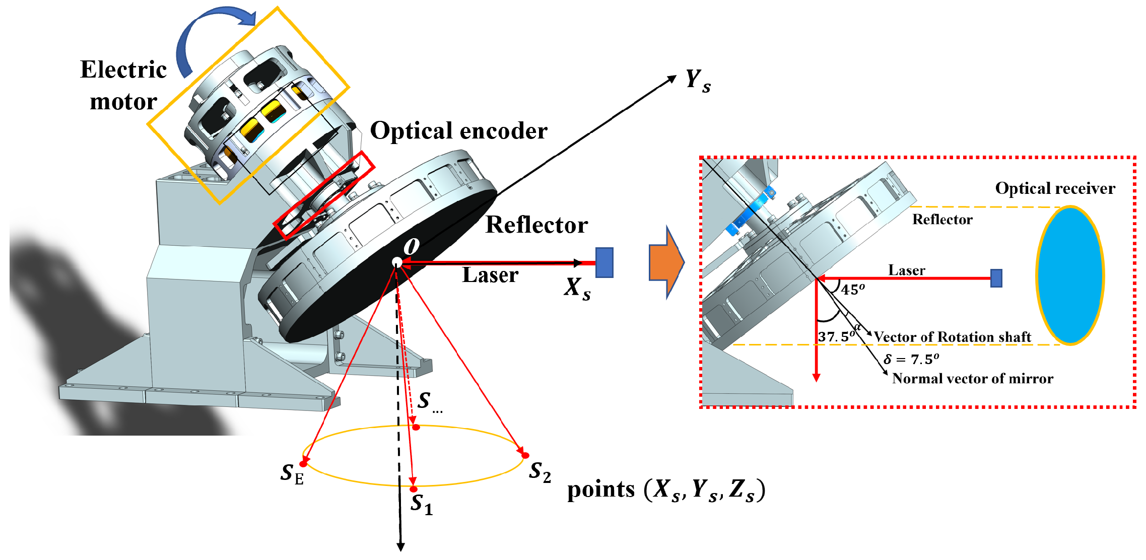
2.2.2. A Palmer Scanning Unit for AHSL

The above illustration shows that the oscillating mirror and rotating mirror methods cannot solve the conflict between optical efficiency and mechanical motors. Thus, the scanning unit in AHSL must integrate the following three features: (1) the minimum edge effect, or the maximum capture of the laser foot point’s field; (2) the minimum $LSP$, ensuring that each emitted laser pulse can be used in an effective scan; and (3) a lower spatial size for mechanical accessibility at the required scanning frequency.

On this basis, we design a Palmer scan unit for AHSL. Figure 3 shows its design.

Figure 3 shows that our Palmer scan unit comprises three main elements: an electric motor, an optical encoder, and a reflecting mirror. The electric motor can rotate at a stable speed of 640 r/min, satisfying the demand for an AHSL system with a scan mirror of a smaller spatial size. The size of the scanning mirror is expressed as Equation (2).

$$V_{palm}={\displaystyle \frac{\pi D^2}{4si{n}^2(37.5^{°})}}·T{h}_{palm}$$

(2)

$T{h}_{palm}$ is the thickness of the scanning mirror. To achieve mechanical stability and simultaneously maintain the stable wave front feature of the mirror’s surface, $T{h}_{palm}$ should be thicker than 3.35 cm to satisfy a rotation speed of 640 r/min [18]. Furthermore, the torque on the surface of the oscillating mirrors is significantly greater than that in the Palmer scan when $T{h}_{palm}$ = $T{h}_{osci}$. Thus, the practical design of $T{h}_{palm}$ can be significantly thinner than $T{h}_{osci}$. Compared to the rotating polygon method, the Palmer scan method cancels out the edge effect, which reduces the field of the laser foot point. Furthermore, our Palmer scanner is coaxial, so a loss of scanning points is caused by the scanning geometry. A quantitative comparison of the three scanning methods is made in

Table 1. Evaluation of scanning methods for AHSL.

Scanning Method	Loss of Scanning Points (LSP)	Motor Load	Quality (Spatial Size)	Edge Effect
Oscillating mirror	0%	High-frequency component	${\displaystyle \frac{\pi D^2}{4si{n}^2\left({30}^{°}\right)}}·Th$	No
Rotating mirror	83.33%	Low-frequency component	$D^3$	Yes
Palmer scan	0%	Low-frequency component	${\displaystyle \frac{\pi D^2}{4si{n}^2(37.5^{°})}}·Th$	No

.

Table 1 shows that the Palmer scan obtains the best performance in all four indexes. The Palmer scan achieves a superior performance with no loss of scanning points, no edge effect, and the lowest mechanical load. Specifically, in terms of the optical efficiency and capacity to capture spectral information, the Palmer scan avoids the loss of effective scan laser foot points when the scan unit is implemented, significantly affecting the point density of AHSL mapping. Furthermore, the Palmer scan method also avoids the edge effect that significantly reduces the efficiency of spectral information capture. Meanwhile, compared to the rotating polygon, the geometry of the Palmer scan method acquires the same optical efficiency using a lightweight scanning mirror that introduces a lighter load on the mechanic motor. Also, the stable rotating scanning of the Palmer method avoids the high-frequency changes in direction of the oscillating mirror. These advantages demonstrate that the Palmer scan method is more feasible in terms of the mechanical load with the required optical aperture. Thus, we conclude that the Palmer scan method is a more practical method for AHSL compared to both rotating polygon and oscillating mirror scanning. Nevertheless, the Palmer scan method includes complex features in its scanning geometry. A model of the scanning geometry of a Palmer scanning unit is given in the next section.

3. Methods

3.1. A Palmer Scanning Model

3.1.1. Palmer Scanning Geometry

The geometry of the scanning unit comprises the orientation of each laser vector $L_{ref}\left(\theta \right)={\left[\begin{array}{ccc}cos{\alpha }_{\theta }& cos{\beta }_{\theta }& cos{\gamma }_{\theta }\end{array}\right]}^T$ at all scanning angles $\theta (\theta \in [0,2\pi \left]\right)$ reflected by the mirror and eventually emitted to the ground. Therefore, the geometry of the Palmer scan is oriented from three individual factors: $N\left(\theta \right)$, the normal vector of the mirror’s surface; $L_{in}\left(\theta \right)$, the orientation of the incident laser; and the law of reflection.

As shown in Figure 3, the main feature of a Palmer scan is that the normal vector of the mirror plane $N\left(\theta \right)$ has a constant angle $\delta$ to the spin axis. In order to obtain a 30° FOV, $\delta$ should be $7.5^{°}$ in the design of a Palmer scanning unit. Then, $N\left(\theta \right)$ rotates around the spin axis with scanning, generating a circular cone. Furthermore, $L_{in}=[1,0,0]$ is a constant vector in AHSL.

Intuitively, two key elements need to be determined to generate the Palmer scan geometry: 1. $N\left(\theta \right)$, the normal vectors of the scanning mirror at all scanning angles. 2. The acquisition of $L_{ref}\left(\theta \right)$ via mapping $N\left(\theta \right)$ onto the function of the specular reflection of the laser beam. Nevertheless, $N\left(\theta \right)=\left[\begin{array}{ccc}cos\theta & sin\theta & -{\displaystyle \frac{1}{tan\delta }}\end{array}\right]$ is difficult to obtain from the intuitive coordinates. These are then rotated into the ground coordinates using the matrix $R_N$, expressed using Equation (3).

$$R_N=\left[\begin{array}{ccc}cos{A}_1& 0& sin{A}_1\\ 0& 1& 0\\ -sin{A}_1& 0& cos{A}_1\end{array}\right]$$

(3)

In the above equation, $A_1$ is the angle between the spin axis and the horizontal direction. In our AHSL setting, $A_1$ is the typical 45°. Thus, the normal vector at all scanning angles is expressed using Equation (4):

$$N\left(\theta \right)=\left[\begin{array}{ccc}{n}_x\left(\theta \right)& n_y\left(\theta \right)& n_z\left(\theta \right)\end{array}\right]={\displaystyle \frac{N_0\left(\theta \right).R_N}{{∥\begin{array}{c}{N}_0\left(\theta \right).R_N\end{array}∥}_2}}$$

(4)

The law of the reflection of a laser beam expressed by $cos{\alpha }_{\theta }=2{(N_{\theta }\times L_{in}^T)}^2-1$ is considered to acquire $L_{ref}\left(\theta \right)$. Then, two equations are given according to the angle conditions.

$$\left[\begin{array}{cc}-n_z\left(\theta \right)& n_y\left(\theta \right)\\ n_y\left(\theta \right)& n_z\left(\theta \right)\end{array}\right]\times \left[\begin{array}{c}cos{\beta }_{\theta }\\ cos{\gamma }_{\theta }\end{array}\right]=\left[\begin{array}{c}0\\ N_{\theta }{L}_{in}^T-n_x\left(\theta \right)cos{\alpha }_{\theta }\end{array}\right]$$

(5)

Considering that the matrix on the left-hand side of the above equation is a positive-definite matrix, the reflected laser vector is expressed using Equation (6):

$$\begin{array}{c}{L}_{ref}\left(\theta \right)\end{array}=\left[\begin{array}{c}2n_x^2\left(\theta \right)-1\\ {\left[\begin{array}{cc}-n_z\left(\theta \right)& n_y\left(\theta \right)\\ n_y\left(\theta \right)& n_z\left(\theta \right)\end{array}\right]}^{-1}\times \left[\begin{array}{c}0\\ n_x\left(\theta \right)(1-cos{\alpha }_{\theta })\end{array}\right]\end{array}\right]$$

(6)

with a combination of $cos{\alpha }_{\theta }$, $N\left(\theta \right)$, and Equation (5). In the actual AHSL system, the resolution of the angle $\Delta \theta$ is determined by the optical encoder. Thus, the orientation of the reflected laser can be acquired with the input of the actual scanning angle $\theta$.

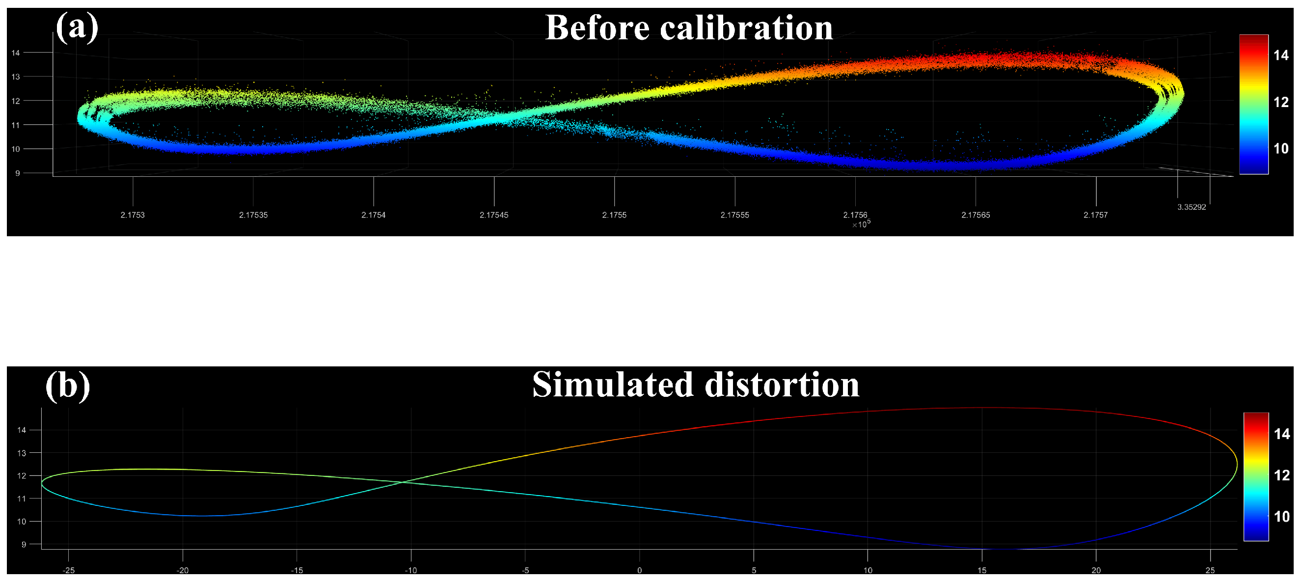
3.1.2. Airborne Palmer Scanning Simulation

An optimized ratio of overlap (ROP) can be acquired by simulating airborne Palmer scanning. Based on the geometry determined in the previous section, a dynamic airborne scan can be simulated using the set of the flight speed (s), height (h), speed of rotation (r), and the rate of repetition of the laser pulse (f). The simulated point cloud is defined by $P(X_p,Y_p)$, where $X_p$ is the coordinate in the direction of flight, and $Y_p$ is the coordinate in the direction of view. The density distributed across the whole scanning strip is described using Equation (7).

$$Den(x,y)=\sum P(P(X_p,Y_p),\lfloor X_p\rfloor =x \&\lfloor Y_p\rfloor =y)$$

(7)

In the above equation, x is the coordinate of the grid in the direction of flight, and y is the coordinate of the grid in the direction of view. $Den(x,y)$ is the number of scanning foot points in each grid $(x,y)$. Then, we can quantify the variation in the density using the coefficient of variation ($CV={\displaystyle \frac{Std}{\overline{Den}}}$) index (the lower, the better). $Std$ and $\overline{Den}$ are the standard deviation and average density values. In addition, these indexes are used to evaluate the quality of airborne scanning strips. With the restriction of acquiring the lowest deviation in density, the best design of the overlap between the strips can be quantitatively explored through iteration of the ratio of overlap (ROP). The $ROP$ is given using Equation (8).

$$ROP={\displaystyle \frac{\Delta D_s}{2h.arctan\frac{FOV}{2}}}(ROP\in [0,0.5])$$

(8)

In the above equation, $\Delta D_s$ is the distance between the center traces of two adjacent strips. The usual design of the $ROP$ is less than 0.5 to maintain redundant observations.

3.2. Scanning Geometry Calibration

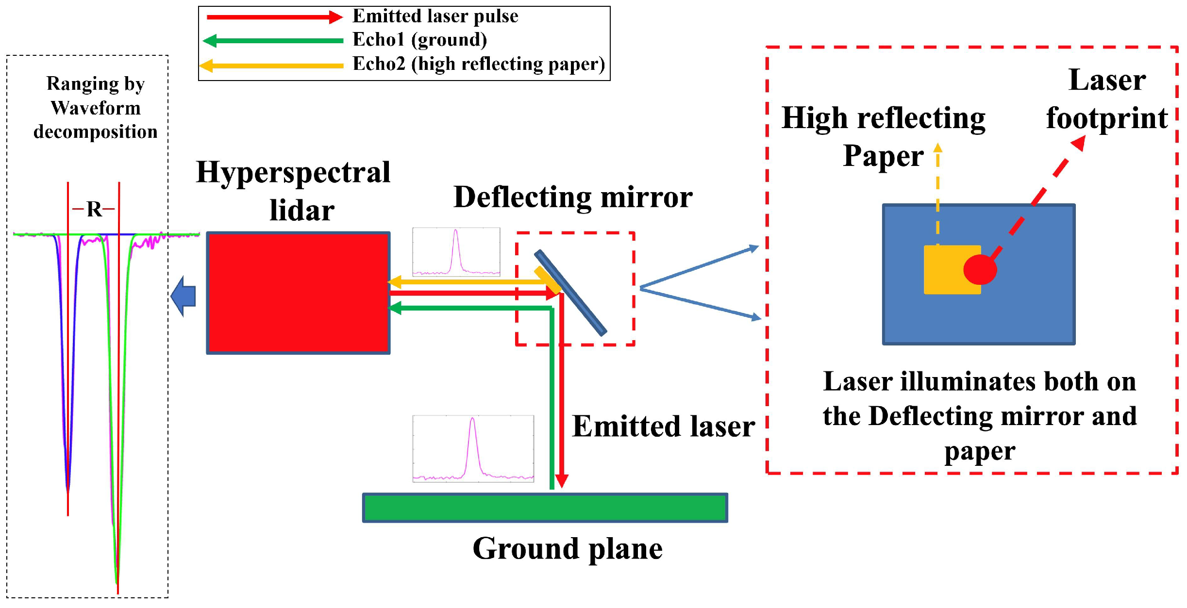
3.2.1. Strategy for Measuring Indoor Self-Orientation Elements

In order to obtain actual laser vectors as the initial elements for indoor orientation in AHSL, due to the larger size and indoor design of the optical receiving unit [18], our AHSL system ranges distances from 0.33 to 670 m. This optical feature makes calibration of the inner orientation elements in an indoor lab accessible. We wish to determine the distance between the scanning center and the laser points. The distance $D\left(\theta \right)$ from the scanning center to the ground is unknown at all scanning angles $\theta$. In addition, it is difficult to acquire using an additional outside measurement device. Thus, this paper proposes a strategy based on the self-ranging feature of AHSL, which is shown in Figure 4.

As shown in Figure 4, a paper with high reflectance and a 0.1 mm thickness is attached to the mirror’s surface to block half of the laser’s footprint. Then, the laser beam illuminates both the high-reflecting paper and the coordinating paper on the ground, which introduces two back-reflected echoes that can be recorded by the hyperspectral LIDAR system. Considering the accessibility of hyperspectral LIDAR itself, $D\left(\theta \right)$ can be retrieved from the dual-waveform echo exhibited in Equation (9).

$$\begin{array}{cc}\hfill I\left(t\right)& =\sum _{i=1}^n{\displaystyle \frac{A}{\sqrt{2\pi }{\sigma }_i}}{e}^{-{\displaystyle \frac{{(t-{\mu }_i)}^2}{2{\sigma }_i^2}}}\hfill \end{array}$$

(9)

In Equation (9), ${\mu }_i$ represents the central position of each backscattered echo, and the range can be determined according to $D={\displaystyle \frac{c}{2}}·({\mu }_2-{\mu }_1)$. According to the research of [23,24], the range’s precision can be improved from 15 mm to less than 1 mm by averaging multiple pulse signals. Thereafter, the scanner’s coordinates $[X_s,Y_s,Z_s]$ and the ground coordinates are defined to measure the laser vector $L_{ref}\left(\theta \right)$. $Y_s$ is in the direction of view, and $X_s$ is in the direction of flight. The laser footprints on the ground are identified using the coordinates $[X_g,Y_g,Z_g]$, and then the laser vector can be expressed using Equation (10).

$$L_{ref}\left(\theta \right)={\displaystyle \frac{P\left(\theta \right)-P_s}{D\left(\theta \right)}}$$

(10)

In the above equation, $P_s=[\Delta X_s,\Delta Y_s,\Delta Z_s]$ is the vector from the center of the scanning mirror to the base point of the ground coordinate system. $[X_g,Y_g]$ can be measured on the indoor ground plane, and $Z_g$ is 0. $D\left(\theta \right)$ is acquired using the self-ranging capability of AHSL, exhibited by ${∥\begin{array}{c}P\left(\theta \right)-P_s\end{array}∥}_2$.

$$D\left(\theta \right)={∥\begin{array}{c}P\left(\theta \right)-P_s\end{array}∥}_2={∥\begin{array}{c}P\left(\theta \right)-[\Delta X_s,\Delta Y_s,\Delta Z_s]\end{array}∥}_2$$

(11)

Thus, the retrieval of $L_{ref}\left(\theta \right)$ can be transferred into the integration of the measurement of $[X_g\left(\theta \right),Y_g\left(\theta \right),Z_g\left(\theta \right)]$, $D\left(\theta \right)$ and the retrieval of $[\Delta X_s,\Delta Y_s,\Delta Z_s]$. As shown by Equation (11), the expression of the retrieval is non-linear. Thus, a non-linear optimizer is required.

The Levenberg–Marquardt (LM) method [25] is a typical non-linear optimizer chosen for iterating and solving the unknown parameter $[\Delta X_s,\Delta Y_s,\Delta Z_s]$. The loss of precision at each measured scanning angle $\theta$ is $\Delta \left(\theta \right)$, and the residual in the whole measurement can be described using Equation (12).

$$min\sum _{i=1}^m|D\left(\theta \right)-{∥\begin{array}{c}P\left(\theta \right)-P_s\end{array}∥}_2|$$

(12)

As illustrated in Figure 4 and Equation (12), we use the advantage of self-ranging with multiple echoes to enhance the accuracy of the distance ranging and use standard record paper to ensure the accuracy of the coordinates. The corresponding model for these elements is also given in the main document, which is expressed as a non-linear equation that can be optimized using the LM algorithm. Through LM optimization, the initial laser vectors can be retrieved using the self-ranging capability of AHSL. It is notable that the range precision can be improved to better than 1 mm by averaging multiple echoes.

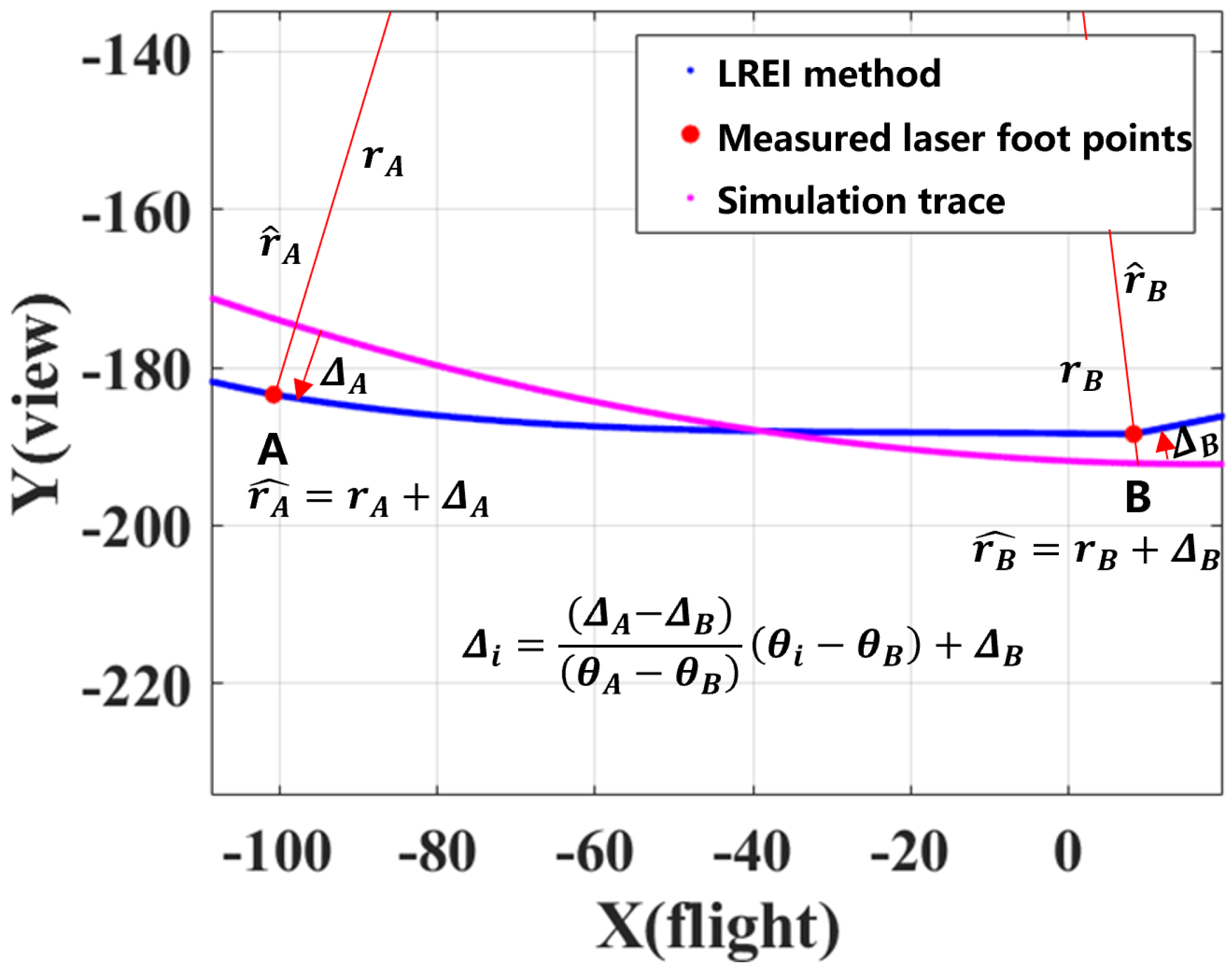
3.2.2. Linear Residual Estimated Interpolation (LREI) for Scanning Traces

Nevertheless, all of the orientation elements should include the laser vectors at all scanning angles measured by the optical encoder. Thus, an interpolation method is inevitably needed to acquire all of the laser vectors from limited laser footprints. Considering that the scan trace of a Palmer scanner is near-elliptic, the typical linear interpolation method exhibited using Equation (13) interpolation is not suitable for interpolating scan traces using limited laser foot point samples.

$${\left[\begin{array}{cc}{X}_i& Y_i\end{array}\right]}^T=\left[\begin{array}{cc}{X}_A& X_B\\ Y_A& Y_B\end{array}\right]{\left[\begin{array}{cc}{\displaystyle \frac{{\theta }_B-{\theta }_i}{{\theta }_B-{\theta }_A}}& 1\end{array}\right]}^T$$

(13)

In the above equation, A is the former scanning point, and B is the latter. i refers to the point that needs to be interpolated. ${\theta }_B$, ${\theta }_A$, and ${\theta }_i$ are, respectively, the scanning angles of points A, B, and i. Nevertheless, linear interpolation will cause the loss of the geometrical features of the Palmer scanning trace. Subsequently, we introduce the linear residual estimated interpolation (LREI) method, a practical and efficient solution based on the Palmer scanning simulation. As demonstrated by Equation (14), LREI efficiently preserves the geometric features of the Palmer scanning trace during the interpolation process. We illustrate the process of the LREI method in Figure 5.

$$\begin{array}{c}{\left[\begin{array}{cc}{X}_i& Y_i\end{array}\right]}^T=(\widehat{r_i}+{\Delta }_i){\left[\begin{array}{cc}cos{\theta }_i& sin{\theta }_i\end{array}\right]}^T\\ \begin{array}{c}{\Delta }_i\end{array}=\left[\begin{array}{cc}(\widehat{r_A}-r_A)& (\widehat{r_B}-r_B)\end{array}\right]{\left[\begin{array}{cc}{\displaystyle \frac{{\theta }_B-{\theta }_i}{{\theta }_B-{\theta }_A}}& 1\end{array}\right]}^T\end{array}$$

(14)

In the above equation, $r_i$, $r_A$, and $r_B$ are the distances from the center projected onto the ground to laser scanning points i, A, and B. ${\Delta }_i$ is the residual distance from the simulated point to the point estimated by our interpolation. In this method, the linear equation estimates the gap based on the residual of point A and point B. Thus, the features of the Palmer scanning trace, expressed by the residual of the simulated trace, can be absorbed into the interpolation process. The LREI method integrates the simulation of the Palmer scanning trace, preserving the geometric features and the convenience of linear interpolation.

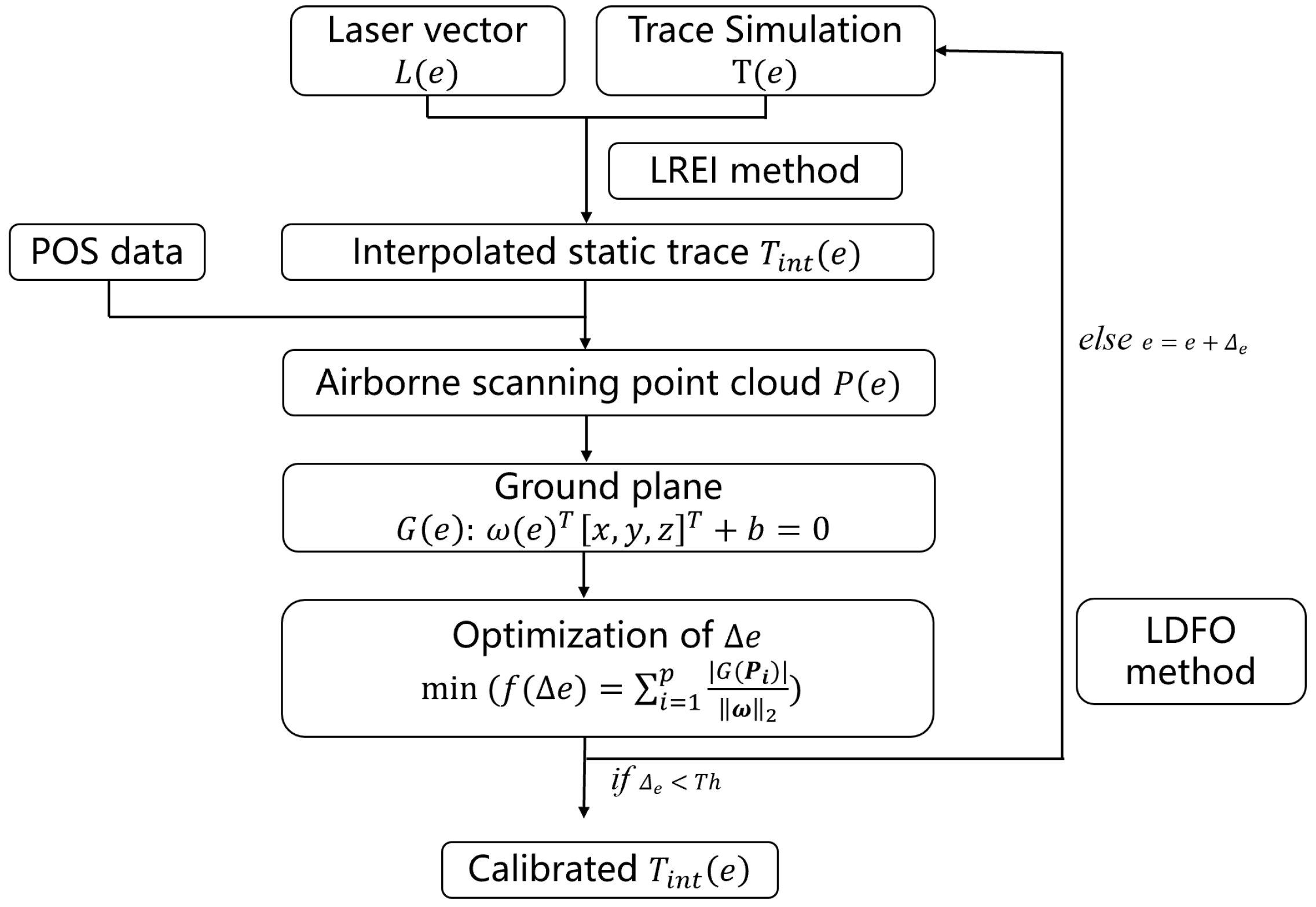
3.2.3. Least-Deviated Flatness Optimization (LDFO) for Angle Offset Calibration

The optical encoder measures the scanning angle, and the initial scanning angle is inconsistent with the initial angle in the standard scanning coordinates. An offset exists between the measured angle ${\theta }_m$ and the actual angle ${\theta }_r={\theta }_m+{\Delta }_e$ in the practical scanning coordinates. Specifically, the scanning angle ${\theta }_m=2\pi {\displaystyle \frac{e}{E}}$ is recorded by the optical encoder with the code $\theta \left(e\right)$. ${\Delta }_e$ is the offset in the scanning angle. e is the code measured by a grating ruler and eventually counted by the optical encoder. E is the maximum code within a whole scanning circle, determined by the resolution of the optical ruler. In our AHSL system, E is 164,840. Considering that the scan trace is near-elliptical, the radius $r_{\theta }$ is significantly unequal at each scanning angle $\theta$. Thus, the angle offset mainly affects the flatness of the scanning trace and the scanning plane, expressed using Equation (15).

$$z_m\left({\theta }_m\right)=z_r\left({\theta }_m\right)+\sqrt{D_r^2-r^2\left({\theta }_r\right)}-\sqrt{D_r^2-r^2\left({\theta }_m\right)}$$

(15)

In the above equation, $z_{\theta }$ is the height of the laser foot points at the scanning angle $\theta$, and $D_r$ is the actual distance from the laser foot point to the scanning center, which is correctly measured by the ranging ability of the AHSL system. $r\left({\theta }_r\right)$ is the distance from the laser point to point $O_g$, which is the vertical projection of the scanning center $O_s$ onto the ground. As the scanning trace on the ground is close to elliptical, it produces a variety of $r\left(\theta \right)$ values. Thus, the measured height of the laser point varies at different scanning angles, resulting in a reduction in the flatness of the scanning ground, which ideally is supposed to be flat.

Then, to retrieve the angle offset and correct its effect on the distortion of the scanning geometry, a method based on least-deviated flatness optimization (LDFO) is proposed. The correction procedure is shown in the following, Figure 6.

The LDFO method shown in Figure 6 is mainly an iteration algorithm that integrates the trace simulation and the LREI method proposed in the previous section. Firstly, based on the simulation of the Palmer scanning model and the self-determined laser vector retrieval strategy, the initial laser vector $L\left(e\right)$ at the separated angle and the scanning trace at all of the scanning angles recorded by the optical encoder can be determined as the initial input data. Then, with the implementation of the LREI method optimized to obtain the complete scanning trace, the interpolated static trace $T_{int}\left(e\right)$ is acquired. To generate a point cloud of the flat ground, an airborne scanning measurement of the airport’s ground is made before the main part of the aerial survey is started. At the same time, the POS data are recorded and processed using the Trimble softwarePOSpac 8.0. Then, the point cloud $P\left(e\right)$ of the airport ground plane is generated. The following, Equation (16), can express the ground plane:

$$G:{\omega }^T{\left[\begin{array}{ccc}x& y& z\end{array}\right]}^T+b=0$$

(16)

In the above equation, $\omega$ is the normalized vector of the generated scanning plane, and $[x,y,z]$ is the laser scanning point measured using AHSL in each iteration. The scanning plane G$\omega$ is fitted using the least-squares algorithm. Thus, the optimization issue can be expressed as the following, Equation (17).

$$minf\left({\Delta }_e\right)=\sum _{i=1}^p{\displaystyle \frac{|{\omega }^T{P}_i|}{{∥\begin{array}{c}\omega \end{array}∥}_2}}$$

(17)

In the above equation, $f\left({\Delta }_e\right)$ represents the variation in flatness, determined by summing the ranges from the laser footprints with the fitting plane G. The angle offset $\Delta \left(e\right)$ is iterated to generate new simulations of the scanning trace until the convergence condition is satisfied.

3.3. The Experimental Setting

The whole experiment is divided into three sub-experiments: simulation of the Palmer scanning model, indoor validation of the LREI method, and airborne validation of correcting the angle offset. The following, Figure 7, exhibits the construction of this framework.

As shown in Figure 7, the experiment is divided into three parts, and their relationship is as follows:

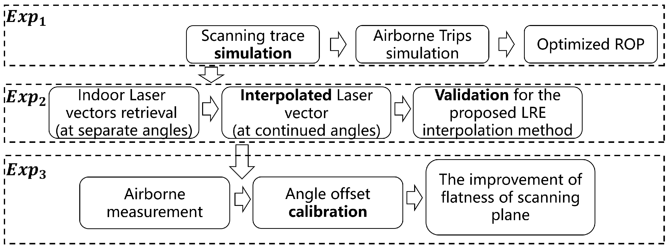
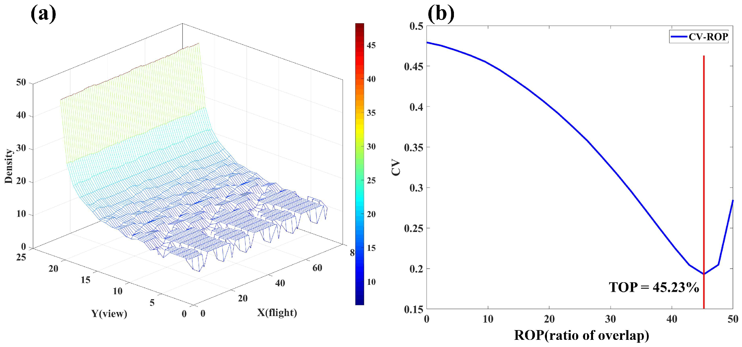
• $exp.1$ Simulation of airborne laser scanning. Firstly, a static scanning trace based on the Palmer model is generated, with indoor laser vector measurements as the input parameters. Secondly, airborne trips are simulated with the input parameters set for an actual aerial survey. Based on the implementation of this step, the optimized rate of overlap (ROP) can be acquired to obtain the least diverse density distribution, providing optimized airborne scanning strip settings.
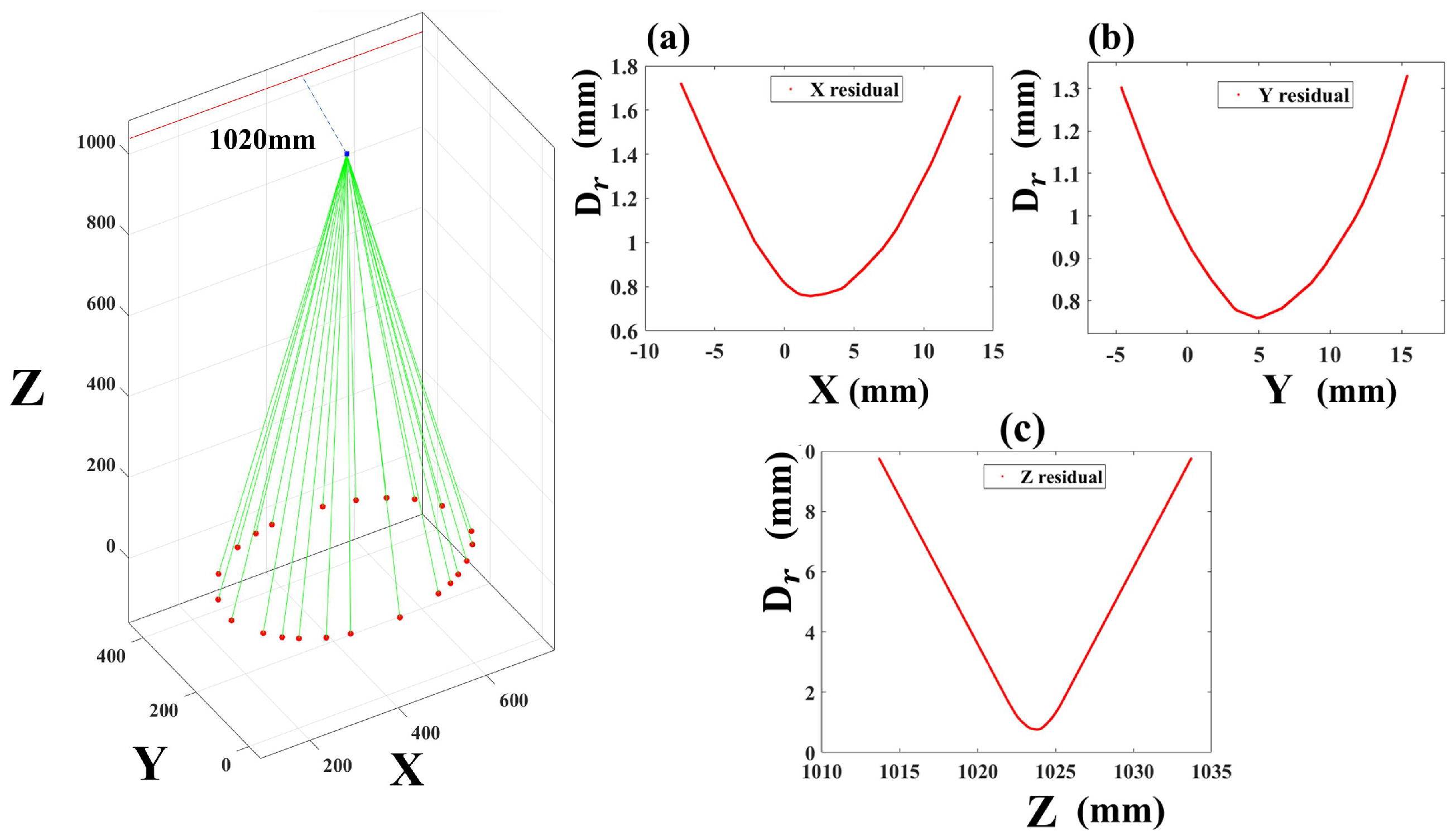
• $exp.2$ Laser vector measurements. Firstly, laser vectors are acquired in several directions. Then, the laser vectors at all scanning angles can be interpolated through the integration of the simulated trace from exp. 1 and the LREI method. A total of 100 points are measured throughout the scanning traces: 30 percent are randomly chosen to interpolate a complete scanning trace, and the other 70 percent are used for validation.
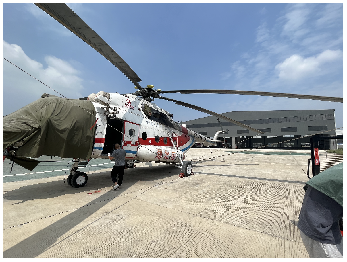
• $exp.3$ Calibration of the initial scanning angle and validation of the proposed calibration method. The effect of the angle offset can be corrected with the scan trace given using LREI in $exp.2$ and LDFO. As airports are usually flat and are inevitably the starting points of aerial survey missions, they are chosen as the ground plane for collecting the point cloud data for calibration in this experiment. The ground truth of the airport and the aerial vehicle for the AHSL system is shown in Figure 8.

This airport is in Hannan district, Wuhan city, Hubei province, China. The rotating speed of the scan mirror is 600/rpm. Furthermore, we note that the measurement starts after the POS unit completes its self-correction.

4. Result

4.1. Simulation and Analysis of Airborne Palmer Scanning

In AHSL, the flight height and flight speed determine the quality of the scan image: a lower cruising speed and flight height create a higher point density. However, a safe flight height in most regions should be greater than 300 m in an aerial mapping mission. Therefore, we simulate scan trips with a 300-m height and a cruising speed of 150 km/h to simulate the mission of a normal aerial survey. Figure 9 shows the simulation of the designed scanning strip with the above flight parameters.

It can be seen above in Figure 9a that the FOV of the scanning strip is 160 m when the height of flight is 300 m. The density of the laser foot point varies from the center of the scanning strip to the edge. The scanning traces consistent with the center line are the sparsest, and the traces at the edge have a relatively higher density. Furthermore, the simulation also exhibits the effect of the angle offset, as shown in Figure 9b. At a flight height of 300 m, the angle offset leads to the worst variation of $\pm 3.4$ m and continuous variation at all scanning angles in the flatness of the 3D imaging. This result indicates that the offset in the scanning angle introduces a significant distortion in the scanning geometry when using the Palmer scan method.

With the simulated strips, the density distribution and the corresponding design of the $ROP$ can be obtained. The results are exhibited in Figure 10.

It can be seen in Figure 10 that the minimum density of 10 points/m² occurs at the center line of the scanning strips. The density increases non-linearly from the center to the edge of the strip. The minimum density within a single scanning strip is 12.7 points/m². Furthermore, as shown in Figure 10b, the minimum coefficient of variation (CV) in the density is obtained when the ROP is designed to be 45.23%. Compared to the original single-scanning-strip strategy, the CV of the designed ROP has been significantly reduced from 0.482 to 0.187.

4.2. Calibration of the Scanning Geometry

4.2.1. Calibration of the Separating Laser Vector

Based on the data acquired through the indoor measurement of the scanning foot points, the orientation from the ground to the scanning center is iterated with the optimization of the LM algorithm. The basic laser vectors can be retrieved. Figure 11 shows the residual curves in the X, Y, and Z directions.

Figure 11 shows that the height of the scanning center is 1020 mm after retrieval. The three valley values in the three residual curves show the precision of the iterations. They are 0.672 mm (0.6588 mrad), 0.705 mm (0.6882 mrad), and 0.891 mm (0.874 mrad) in the spatial directions of x, y, and z. The residuals are all lower than 1 mrad thanks to the contribution of the laser foot points measured for calibration, which provide redundant information for LM optimization. Furthermore, the residual curves in all three dimensions are shown in Figure 11b. Compared to the residuals in the x and y directions, the residual error in the z direction, the direction of height, shows the most significant slope. This result is consistent with the simulation of the Palmer scanning model, considering that height (in the z dimension) is the most significant component of the laser vector.

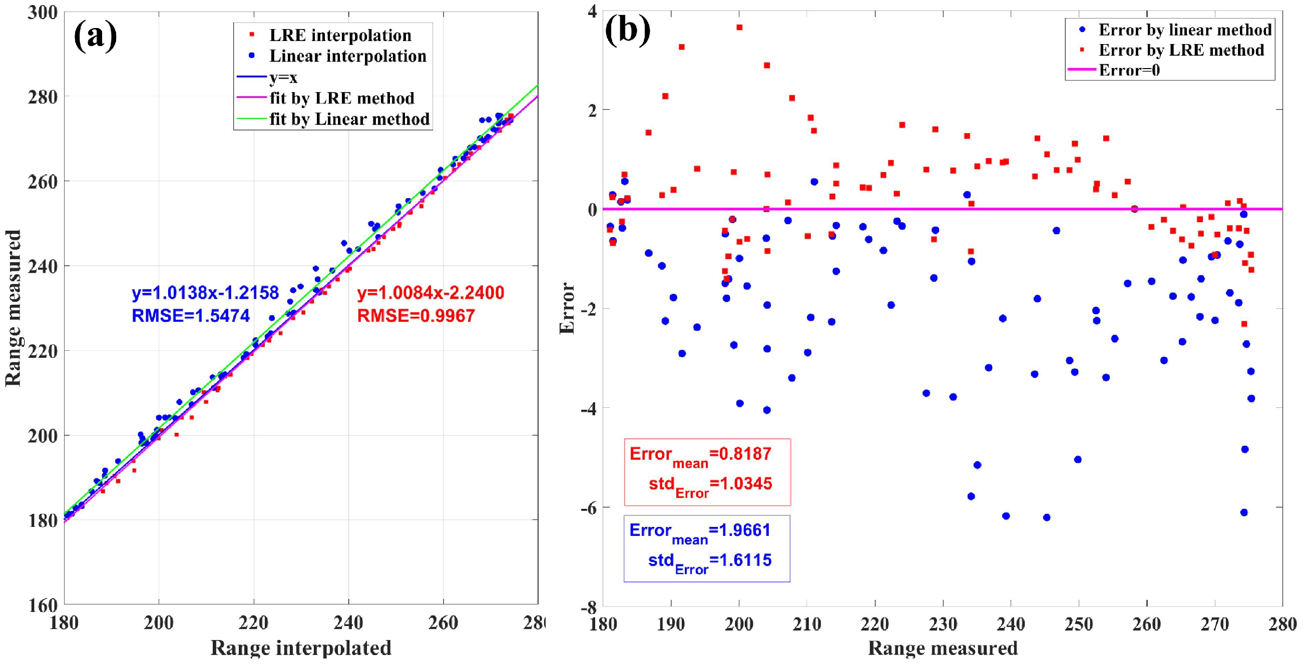
4.2.2. Validation of the LRE Interpolation Method

In order to validate the effect of the LRE interpolation method, 100 laser foot points are uniformly measured within the whole scanning trace with steps of 3.6 degrees. A proportion of 20% of them are chosen as the input for interpolating the complete scanning trace, and the remaining 80% of them are chosen for validating the precision of interpolation by comparing the typical linear interpolation method and the spline method. The results of interpolation using the two methods are exhibited in the following, Figure 12.

It can be seen from Figure 12 that the trace generated using the LRE interpolation method is more consistent with the laser points for validation. This shows that the LREI method maintains the geometrical features of the Palmer trace. Specifically, Figure 12 exhibits the significant error of the LI method: it can be seen that in this case, the error of the LREI method is 0.839 mm (0.823 mrad), while the typical linear method acquires 6.257 mm (6.134 mrad) of the range to the center, reducing 86.58% of the error. In addition, the trace interpolated using the spline method is also exhibited in Figure 12. We separate the coordinates into two groups, each of which includes an x-y dataset in the form of a normal function. Thus, the spline method can be utilized to interpolate the entire scan trace. Nevertheless, obvious distortion of the interpolated trace occurs at the end of each part, with significant growth of the slope. Furthermore, it can be seen in the right-hand side of Figure 12 that in this case, the spline method creates a significant distortion, with an error of 9.318 mrad. To quantitatively validate the effect of the interpolation methods throughout the scanning trace, we collected the error for each interpolated laser point and mapped the results in the following, Figure 13.

In Figure 13a, the points interpolated using the typical linear method are fitted by the green curve, which are obviously overestimated compared to those in the LREI method. The average error in the interpolation using the LREI method is 0.8187 mm (0.8026 mrad), while it is 1.9661 mm (1.9275 mrad) when using the linear method. This shows that our LREI method can significantly reduce the error to less than 50% of that in the linear method. Furthermore, the standard deviation in the bias and the RMSE of the whole interpolation, representing the stability of the LREI method, are lower than those of the typical linear method. The standard deviation in the bias when using the LREI method is 1.611 mm (1.579 mrad), while the LREI method obtains 1.035 mm (1.014 mrad). The lowest root mean square error (RMSE) of the LREI method is 0.996 mm (0.977 mrad), which is 35.59% lower than the 1.547 mm (1.517 mrad) with the linear interpolation method. The above result proves that the LREI method can significantly reduce the interpolation error.

4.2.3. Calibration of the Angle Offset

The point cloud of the ground plane used to correct the effect of the angle offset is generated and shown in Figure 14. The offset of the scanning angle is determined using the LDFO method. Scanning point clouds of the ground plane before correction and after correction are exhibited in the following, Figure 14.

It can be seen in Figure 14a that the distortion of the point cloud is consistent with the results exhibited by the simulation, the points of which are in the shape of a saddle. After the correction of the angle offset, the point cloud is flatter. A quantitative comparison of before–after correction is shown in

Table 2. The improvement in the flatness after correction.

	Standard Deviation of Flatness	Worst Deviation of Flatness
Before correction	1.389 m	6.4 m
After correction	0.241 m	1.953 m

.

It can be seen from Table 2 that after calibration of the angle offset, the flatness of the point cloud obtains a lower standard deviation of 0.2406 m, compared to the 1.389 m deviation before calibration. Furthermore, the worst deviation in the flatness is reduced from 6.4 to 1.9525 m, with a reduction in the variation of 69.5%. This result indicates that the precision of the flatness and the scanning geometry has been significantly improved.

5. Discussion

In terms of the Palmer scanning simulation, it can be seen from the results of the simulation of the scanning strip that the middle region of the strip is significantly sparser than the edge region. This issue introduces a deviation in the point density within the scan strip. Optimization of the ROP permits the least deviation in the point density of mapping when the two neighboring scan strips overlap. A ROP higher than the optimized value results in a decrease in the homogeneity of the point cloud’s density, which is indicated by the CV. Therefore, an optimized ROP avoids a redundant overlap, with a suitable scanning efficiency.

The initial laser vectors are retrieved. The LREI method proposed in this work aims to complete the scanning traces. The initial input for LREI can be set to 20–30% of the laser foot points of the static traces with indoor self-calibration. As illustrated in Figure 12, we use 20 points as the initial input. The trace interpolated using the LREI method is iteratively optimized through the LDFO process. The input of LDFO is the scan trace obtained while the helicopter is in hold-on status before a flight mission. Thus, the data input of the LREI method will not significantly increase with the expansion of the total mapping scale. It is seen from the results of the interpolation that compared to the linear interpolation method, the LREI method provides a closer estimation of the scan trace. Furthermore, the distortion caused by the spline method may be related to its cubic polynomial property and functional form. The rapid growth of the function slope leads to poor performance in smoothing. This result supports the notion that the LREI method effectively utilizes the interior information of the residual error between the simulation trace and the measured points to estimate the entire interpolation trace. With the simulation of the original Palmer scan being the basic function of the interpolation, the LREI method estimates the residual error to fit the measured points, which preserves the basic geometric features of the Palmer scan.

We correct the angle offset using the LDFO algorithm. The range precision (per pulse) of AHSL in an actual aerial survey is 0.15 m. This result indicates that the standard deviation in the scanning plane is greater than 0.15 m. It can be seen from the simulation that the deviation caused by the angle offset is less than 2% height, which means a height higher than 7.5 m is required to perform the calibration. Thus, calibration of the offset of the scanning angle cannot be effectively implemented indoors. Therefore, the scanned point cloud for this calibration needs to be collected under airborne conditions. Furthermore, the scanned point cloud of the ground plane exhibits the approximate features of the simulation results. The offset of the scanning angle is retrieved to be 87.357 degrees using the LDFO method. Then, we simulate a static scan trace with an angle offset of 87.357 degrees, and the corresponding height is set to the same value as the actual measurement. The result of the simulation is exhibited in the following, Figure 15.

As shown in the above, Figure 15, the point cloud of the scanned ground exhibits the same features as those in the simulated trace. Furthermore, the worst variation in flatness shown in Figure 15a is 6.203 m. And the worst actual variation in flatness is 6.4 m. This result indicates that the main component that distorts the flatness is the angle offset. The range precision is 0.15 m, which mainly controls the 0.190 m (bias) between the simulated and scanned traces. The LDFO algorithm in this work plays a crucial role in the iterative calibration of the laser vectors and the angle offset before each flight mission. We assume that the ground plane used in this section is flat for two reasons. On the one hand, most helicopter airports are flat and highly horizontal, which makes them naturally suitable for LDFO calibration. Thus, the LDFO method proposed in this work can be operated without further adjustments. On the other hand, the helicopter needs a period to set the flight route and to initialize its sensors. Researchers can use this period to scan the ground plane to obtain the data for the LDFO process. Furthermore, for some extreme cases, such as under rapid variation in the terrain’s elevation and the complexity of the 3D environment, where there is no suitable place for an ideally complete input scene, the input of the LDFO algorithm can be set as a combination of a series of fragmented scenes, each of which is a relatively flat plane. This issue will cause the goal of convergence in the LDFO algorithm to turn into the least deviation in the flatness of each partially scanned scene. The choice and power settings of these fragmented planes should be considered in such scenarios. There are also some potential challenges in future calibration work. Firstly, the metadata of the POS data need to be deeply integrated with the scanning geometry to avoid systematic errors being caused by the IMU. Secondly, the regular region or targets should be considered as ground control points for calibrating the residual errors in trace interpolation further. To address these challenges, the advantage of the 3D spectral point cloud generated by AHSL itself will become a natural aid for matching visible-light images for further calibration. A visible-light camera and the resolution of image matching issues are crucial for further calibration of AHSL. AHSL can image a 3D spectral point cloud covering the visible-light band, which means that further calibration of the potential geometry can take satellite or unmanned aerial vehicle (UAV) images in the matching region as s reference. Auto-calibration methods that use integrated spatial–spectral information are promising for developing the calibration process detailed further.

6. Conclusions

This work focuses on providing a practical scanning method and calibrating the scanning geometry for airborne hyperspectral LiDAR (AHSL). We introduce and analyze novel issues in the scanning method for AHSL: the mechanical–optical trade-off. Simulations of the typical scan methods are implemented and the scanning geometry calibrated.

Our findings reveal that Palmer scans can significantly reduce the high-frequency component of the mechanical load and improve the quality of the mirror in terms of its mass compared to that in the oscillating mirror method. Moreover, the Palmer scanning method effectively reduces 86.6% of the loss of the emitted laser pulse and eliminates the edge effect on the distortion of the reflecting spectrum that occurs with the rotating polygon method.

In calibrating the scanning geometry of the Palmer scan method, we notice and take advantage of the large optical aperture in AHSL to achieve a self-ranging capability. We propose a three-step strategy for tackling this issue: an indoor self-retrieval method for acquiring the primary inner orientation elements, interpolating the static scanned traces, and correcting the offset in the scanning angle. This comprehensive approach ensures the accuracy and reliability of our calibration.

Firstly, the indoor self-retrieval strategy measures the initial laser vectors and retrieves the orientation elements from indoor measurements of the laser scan points by the LM optimizer. The results show that the precision is less than 1 mrad (to the range), with improvements through multiple-pulse ranging utilized in these measurements.

Secondly, a linear residual estimated interpolation (LREI) method is proposed for reducing the distortion produced by the interpolation process. The LREI method utilizes the simulation and orientation of the laser points provided by the indoor measurement from the first step. Compared to the typical linear interpolation method, our method can reduce the RMSE of the interpolation from 1.517 to 0.977 mrad. Furthermore, the simulation revealed that the lowest coefficient of variation (CV) for the density is obtained when the ratio of overlap (ROP) is 45.23%. Based on this finding, an optimized flight design can be indicated. Flight height and speed are two crucial parameters that linearly influence the density of the points. The data in this work also provide a reference for further simulations of operating under different flight conditions.

Thirdly, we explore the effect of the scanning angle offset on the distortion of the scanned plane in the direction of height through simulations. We propose an iterative method, least-deviated flatness optimization (LDFO), for calibrating this effect. After correction, the standard deviation in the flatness is reduced from 1.389 m to 0.241 m, and the worst variation in the flatness is reduced from 6.4 m to 1.953 m.

According to our vision, we suggest a few significant potential directions for the development of calibration methods for AHSL. Firstly, we suggest the deep integration of multi-source sensor data, especially POS metadata, into the calibration model to include more dynamic elements in aerial surveys. Secondly, we envision the implementation of scanning image calibration with a set of regular targeting zones based on a fused model. Auto-calibration methods that utilize spatial–spectral information are promising for developing the calibration process detailed further.

References

1. Telling, J.W.; Lyda, A.; Hartzell, P.J.; Glennie, C.L. Review of Earth science research using terrestrial laser scanning. Earth-Sci. Rev. 2017, 169, 35–68. [Google Scholar] [CrossRef]
2. Matikainen, L.; Karila, K.; Hyyppä, J.; Litkey, P.; Puttonen, E.; Ahokas, E. Object-based analysis of multispectral airborne laser scanner data for land cover classification and map updating. Isprs J. Photogramm. Remote Sens. 2017, 128, 298–313. [Google Scholar] [CrossRef]
3. Glennie, C.L.; Carter, W.E.; Shrestha, R.L.; Dietrich, W.E.J. Geodetic imaging with airborne LiDAR: The Earth’s surface revealed. Rep. Prog. Phys. 2013, 76, 086801. [Google Scholar] [CrossRef]
4. Lu, B.; Dao, P.D.; Liu, J.; He, Y.; Shang, J. Recent Advances of Hyperspectral Imaging Technology and Applications in Agriculture. Remote Sens. 2020, 12, 2659. [Google Scholar] [CrossRef]
5. Kim, Y.; Kim, Y. Improved Classification Accuracy Based on the Output-Level Fusion of High-Resolution Satellite Images and Airborne LiDAR Data in Urban Area. IEEE Geosci. Remote Sens. Lett. 2014, 11, 636–640. [Google Scholar]
6. Zhao, X.; Qi, J.; Xu, H.; Yu, Z.; Yuan, L.; Chen, Y.; Huang, H. Evaluating the potential of airborne hyperspectral LiDAR for assessing forest insects and diseases with 3D Radiative Transfer Modeling. Remote Sens. Environ. 2023, 297, 113759. [Google Scholar] [CrossRef]
7. Dansona, M.; Gaultonb, R.; Armitagea, R.P.; Disneyc, M.; Lewisc, P.; Pearsone, G.; Ramireza, A.F. Developing a dual-wavelength full-waveform terrestrial laser scanner to characterize forest canopy structure. Agric. For. Meteorol. 2014, 198–199, 7–14. [Google Scholar] [CrossRef]
8. Leigh, H.W.; Magruder, L.A. Using dual-wavelength, full-waveform airborne lidar for surface classification and vegetation characterization. J. Appl. Remote Sens. 2016, 10, 045001. [Google Scholar] [CrossRef]
9. Diaz, J.C.F.; Carter, W.E.; Glennie, C.L.; Shrestha, R.L.; Pan, Z.; Ekhtari, N.; Singhania, A.; Hauser, D.L.; Sartori, M.P. Capability Assessment and Performance Metrics for the Titan Multispectral Mapping Lidar. Remote Sens. 2016, 8, 936. [Google Scholar] [CrossRef]
10. Shi, S.; Bi, S.; Gong, W.; Chen, B.; Chen, B.; Tang, X.; Qu, F.; Song, S. Land Cover Classification with Multispectral LiDAR Based on Multi-Scale Spatial and Spectral Feature Selection. Remote Sens. 2021, 13, 4118. [Google Scholar] [CrossRef]
11. Shi, S.; Tang, X.; Chen, B.; Chen, B.; Xu, Q.; Bi, S.; Gong, W. Point Cloud Data Processing Optimization in Spectral and Spatial Dimensions Based on Multispectral Lidar for Urban Single-Wood Extraction. ISPRS Int. J. Geo Inf. 2023, 12, 90. [Google Scholar] [CrossRef]
12. Gong, W.; Sun, J.; Shi, S.; Yang, J.; Du, L.; Zhu, B.; Song, S. Investigating the Potential of Using the Spatial and Spectral Information of Multispectral LiDAR for Object Classification. Sensors 2015, 15, 21989–22002. [Google Scholar] [CrossRef]
13. Gong, W.; Shi, S.; Chen, B.; Song, S.; Niu, Z.; Wang, C.; Guan, H.; Li, W.; Gao, S.; Lin, Y.; et al. Development and prospect of hyperspectral LiDAR for earth observation. Nat. Remote Sens. Bull. 2021, 25, 501–513. [Google Scholar] [CrossRef]
14. Qian, L.; Wu, D.; Liu, D.; Song, S.; Shi, S.; Gong, W.; Wang, L. Parameter Simulation and Design of an Airborne Hyperspectral Imaging LiDAR System. Remote Sens. 2021, 13, 5123. [Google Scholar] [CrossRef]
15. Qian, L.; Liu, D.; Zhu, X. Laser projection optical path design and speckle suppression. In Proceedings of the Fourteenth National Conference on Laser Technology and Optoelectronics, Shanghai, China, 17–20 March 2019. [Google Scholar]
16. Qian, L.; Wu, D.; Liu, D.; Zhong, L.; Shi, S.; Song, S.; Gong, W. Design and demonstration of airborne hyperspectral imaging LiDAR system based on optical fiber array focal plane splitting. Opt. Commun. 2023, 534, 129331. [Google Scholar] [CrossRef]
17. Wang, B.; Song, S.; Shi, S.; Chen, Z.; Li, F.; Wu, D.; Liu, D.; Gong, W. Multichannel Interconnection Decomposition for Hyperspectral LiDAR Waveforms Detected from over 500 m. IEEE Trans. Geosci. Remote Sens. 2022, 60, 1–14. [Google Scholar] [CrossRef]
18. Qian, L.; Wu, D.; Zhou, X.; Zhong, L.; Wei, W.; Wang, Y.; Shi, S.; Song, S.; Gong, W.; Liu, D. Optical system design for a hyperspectral imaging lidar using supercontinuum laser and its preliminary performance. Optics Express 2021, 29 11, 17542–17553. [Google Scholar] [CrossRef]
19. Wehr, A.; Lohr, U. Airborne laser scanning—An introduction and overview. Isprs J. Photogramm. Remote Sens. 1999, 54, 68–82. [Google Scholar] [CrossRef]
20. Wei, Y. Analysis and implementation of limited angle swing scanning control system. Infrared Laser Eng. 2007, 36, 357. [Google Scholar]
21. Rong, S. Method of achieving uniform scanning of airborne lidar. Infrared Laser Eng. 2008, 37, 675. [Google Scholar]
22. Brosens, P.J. Scanning speed and accuracy of moving magnet optical scanners. In Recording Systems: High-Resolution Cameras and Recording Devices and Laser Scanning and Recording Systems; SPIE: Bellingham, WA, USA, 1993. [Google Scholar]
23. Song, S.; Wang, B.; Gong, W.; Zhenwei, C.; Xin, L.; Sun, J.; Shi, S. A new waveform decomposition method for multispectral LiDAR. Isprs J. Photogramm. Remote Sens. 2019, 149, 40–49. [Google Scholar] [CrossRef]
24. Shi, S.; Gong, C.; Xu, Q.; Wang, A.; Tang, X.; Bi, S.; Gong, W. Waveform Information Accurate Extraction for Massive and Complex Waveform Data of Hyperspectral Lidar. IEEE J. Sel. Top. Appl. Earth Obs. Remote Sens. 2025, 18, 1020–1038. [Google Scholar] [CrossRef]
25. Madsen, K.; Nielsen, H.B.; Tingleff, O. Methods for Non-Linear Least Squares Problems; Technical University of Denmark: Kongens Lyngby, Denmark, 1999. [Google Scholar]
Figure 1. The construction of the airborne hyperspectral LiDAR system. (a) Design of the AHSL system. (b) Exhibition of the AHSL system.
Remotesensing 17 01450 g001
Figure 2. The typical scanning models for ASL. (a) The working mechanism of the oscillating mirror method; (b) the working mechanism of the rotating polygon method.
Remotesensing 17 01450 g002
Figure 3. The design of the Palmer scanning unit.
Remotesensing 17 01450 g003
Figure 4. Measurement of laser vectors and retrieval of the center of the geometry in scanning coordinates.
Remotesensing 17 01450 g004
Figure 5. The procedure of iteration for the angle offset.
Remotesensing 17 01450 g005
Figure 6. The procedure of iteration for the angle offset using the LDFO method.
Remotesensing 17 01450 g006
Figure 7. The framework of the experiment.
Remotesensing 17 01450 g007
Figure 8. The aircraft load and the airport for the flight mission.
Remotesensing 17 01450 g008
Figure 9. Airborne simulation of the Palmer scan. (a) Simulation of the scan strip; (b) simulation of the trace distortion.
Remotesensing 17 01450 g009
Figure 10. Distribution of the point density in the Palmer scan. (a) The density distribution of the scan points on the scan strip. (b) The CV coefficient with the variation in the ROP. The red line in (b) indicates the lowest CV.
Remotesensing 17 01450 g010
Figure 11. The precision of initial laser vector retrieval. (a) The residual curve in the direction of coordinate X; (b) the residual curve in the direction of coordinate Y; (c) the residual curve in the direction of coordinate Z.
Remotesensing 17 01450 g011
Figure 12. The interpolation of Palmer traces. The red arrows indicate the errors of interpolation using the different methods.
Remotesensing 17 01450 g012
Figure 13. Accuracy of interpolation using the linear method and the LREI method. (a) Validation curves of the accuracy of the two interpolation methods. (b) The error distributions of the two interpolation methods.
Remotesensing 17 01450 g013
Figure 14. The effect of AO calibration on the point cloud. (a) The scan trace before calibration. (b) The scan trace with the calibration of the LDFO method.
Remotesensing 17 01450 g014
Figure 15. Measured and simulated distortion in the scanning strip. (a) The scanning strip before calibration. (b) Scanning strip simulation with the retrieved angle offset parameter.
Remotesensing 17 01450 g015