Evaluation of Different Methods for Retrieving Temperature and Humidity Profiles in the Lower Atmosphere Using the Atmospheric Sounder Spectrometer by Infrared Spectral Technology

Abstract

The temperature and humidity profiles within the planetary boundary layer (PBL) are crucial for Earth’s climate research. The Atmospheric Sounder Spectrometer by Infrared Spectral Technology (ASSIST) measures downward thermal radiation in the atmosphere with high temporal and spectral resolution continuously during day and night. The physics-based retrieval method, utilizing iterative optimization, can obtain solutions that align with the true atmospheric state. However, the retrieval is typically an ill-posed problem and is affected by noise, necessitating the introduction of regularization. To achieve high-precision detection, a systematic evaluation was conducted on the retrieval performance of temperature and humidity profiles using ASSIST by regularization methods based on the Gauss–Newton framework, which include Fixed regularization factor (FR), L-Curve (LC), Generalized Cross-Validation (GCV), Maximum Likelihood Estimation (MLE), and Iterative Regularized Gauss–Newton (IRGN) methods, and the Levenberg–Marquardt (LM) method based on a damping least squares strategy. A five-day validation experiment was conducted under clear-sky conditions at the Anqing radiosonde station in China. The results indicate that for temperature profile retrieval, the IRGN method demonstrates superior performance, particularly below 1.5 $\mathrm{k}\mathrm{m}$ altitude, where the mean BIAS, mean RMSE, mean Degrees of Freedom for Signal (DFS), and mean residual reach 0.42 $\mathrm{K}$, 0.80 $\mathrm{K}$, 3.37, and $3.01\times {10}^{-13}$ $\left(\mathrm{W}/{\mathrm{c}\mathrm{m}}^2 \mathrm{s}\mathrm{r} {\mathrm{c}\mathrm{m}}^{-1}\right)$, respectively. In contrast, other regularization methods exhibit over-regularization, leading to degraded information content. For humidity profile retrieval, below 1.5 $\mathrm{k}\mathrm{m}$ altitude, the LM method outperforms all regularization-based methods, with the mean BIAS, mean RMSE, mean DFS, and mean residual of 3.65$\%$, 5.62$\%$, 2.05, and $4.36\times {10}^{-12}$ $\left(\mathrm{W}/{\mathrm{c}\mathrm{m}}^2 \mathrm{s}\mathrm{r} {\mathrm{c}\mathrm{m}}^{-1}\right)$, respectively. Conversely, other regularization methods exhibit strong prior dependence, causing retrieval to converge results toward the initial guess.

1. Introduction

Temperature and humidity profiles within the planetary boundary layer (PBL) have a large impact on the Earth’s climate system and weather processes. These profiles provide detailed information on the variations in temperature and humidity with altitude, which are of significant importance in various fields, such as understanding energy and water cycles, weather forecasting, climate monitoring, and the initialization of numerical weather prediction (NWP) models [1,2,3,4]. As science and technology advance, the demand for continuous and high-resolution PBL measurements has increased to improve the accuracy of weather forecasting and the reliability of climate models.

Traditional atmospheric detection methods, such as radiosondes, provide relatively accurate information about the vertical structure of the atmosphere. However, their low temporal resolution (several times per day) limits their capacity to capture rapidly changing atmospheric phenomena [5,6]. Lidar measurements provide precise and high-resolution atmospheric profile detection. However, different radar technologies face multiple challenges in practical applications, including environmental adaptability, signal noise, hardware calibration, and the complexity of data processing [7,8,9,10]. Microwave measurements exhibit high sensitivity to the atmosphere above 15 $\mathrm{k}\mathrm{m}$ but show limited accuracy in detecting the boundary layer [11]. Spaceborne measurements provide wider spatial coverage and higher horizontal resolution. However, satellite observations remain insufficient for resolving structures within the PBL, as they are primarily sensitive to the upper PBL [1]. Ground-based infrared hyperspectral technology, with high temporal and moderate vertical resolution, measures the downward infrared radiation emitted by the atmosphere, providing a new observational approach for studying the structure and dynamics of the PBL.

Ground-based infrared hyperspectral instruments are generally categorized into two main types. One type includes Fourier Transform Infrared (FTIR) instruments, which primarily use high-resolution near-infrared and mid-infrared solar spectra to retrieve atmospheric profiles, such as those deployed in the Network for the Detection of Atmospheric Composition Change (NDACC) [12,13]. The other type includes instruments that primarily use downward thermal radiation from the atmosphere to retrieve atmospheric profiles, such as the Atmospheric Emitted Radiance Interferometer (AERI) deployed in the Atmospheric Radiation Measurement (ARM) program [14] and the Atmospheric Infrared Sounder Spectrometer (ASSIST) developed by LR Tech [15,16]. FTIR instruments use high-resolution near-infrared and mid-infrared solar spectra to retrieve water vapor and various trace gas profiles or column concentrations [17,18], which make them unsuitable for nighttime observations. The AERI and ASSIST primarily collect downward thermal radiation emitted by the atmosphere, allowing for continuous observations both day and night. The AERI covers nearly the entire thermal infrared spectrum (520–3000 ${\mathrm{c}\mathrm{m}}^{-1}$) with a temporal resolution of 8 min. It is capable of measuring various atmospheric components, including temperature and humidity [19], greenhouse gases [20], aerosols [21], and clouds [18]. Compared to the AERI, the ASSIST offers a higher temporal resolution (2 min) and a broader spectral range (520–3300 ${\mathrm{c}\mathrm{m}}^{-1}$) and can also perform continuous measurements of various atmospheric components during both day and night [15,22].

Extracting atmospheric profile information from thermal infrared spectra typically involves two types of retrieval algorithms: statistical methods based on regression and machine learning and iterative optimization strategies based on physical models. Regression-based statistical retrieval offers fast processing speeds, though with lower accuracy [23]. In contrast, machine learning methods can achieve a highly accurate nonlinear mapping from observations to retrieval profiles [5,24,25,26]. An increasing number of machine learning methods incorporating physical constraints are being applied in atmospheric physics research [27,28]. Nevertheless, machine learning methods based on physical constraints have high training costs and significant computation complexity. Moreover, the atmospheric environment exhibits significant dynamic variations, which affect the model’s ability to generalize across diverse scenarios. Conversely, physics-based iterative methods based on atmospheric radiative transfer models can provide solutions that better reflect the true state of the atmosphere. Since the atmospheric profile retrieval is inherently an ill-posed problem, and the noise present during the measurement process can lead to significant errors in the retrieval of results. Regularization is required to introduce constraints that stabilize the solution and ensure its physical validity [29,30].

The selection of the regularization factor in atmospheric profile retrieval is crucial and challenging. Currently, the selection of regularization parameters in atmospheric nonlinear retrieval primarily follows two main classes: explicit regularization methods based on the Gauss–Newton framework and the damped least squares method with implicit stabilization effects. The former directly introduces a regularization term by modifying the objective function and includes methods such as empirical assignment [31], Expected Error Estimation (EEE) [29], Discrepancy Principle (DP) [32,33], Generalized Cross-Validation (GCV) [34], Maximum Likelihood Estimation (MLE) [35], L-Curve (LC) [36,37], and Iterative Regularized Gauss–Newton (IRGN) [29]. The latter is represented by the Levenberg–Marquardt (LM) method [38,39,40,41], which, although not explicitly incorporating a regularization term, introduces a diagonal increment in the Hessian matrix by dynamically adjusting the damping factor. This approach combines the convergence efficiency of the Gauss–Newton method with the stability of the gradient descent method. Turner et al. [19] used the AERI to retrieve temperature and humidity profiles, applying fixed regularization factors (1000, 300, 100, 30, 10, 3, and 1) during the iterative process to balance prior information and observational data. This empirical approach exhibits considerable subjectivity and lacks theoretical foundation. The EEE method selects the regularization parameter by minimizing the expected error. This method is based on statistical estimates of smoothing errors, noise errors, and model errors. However, it relies on prior information and has a high computational cost. The DP method selects the optimal regularization parameter by matching the squared residual to the assumed noise level. It is effective when the noise level is known, but requires careful adjustment of the control parameters $\chi$. The GCV selects the regularization parameter by minimizing a cross-validation function that includes both the residual norm and a “degrees of freedom” term. A challenge arises when the minimum of the cross-validation function is too flat, making precise selection difficult. The MLE estimates the optimal regularization parameter by minimizing the maximum likelihood function, which includes both the residual and the Jacobian matrix. Nevertheless, it can sometimes lead to under-regularized solutions. The LC method selects the regularization factor $\gamma$ at the corner of the L-shaped curve to minimize the combination of the regularization term and the residual term, but it may result in over-regularization, especially in high-noise conditions. Iterative regularization methods are becoming increasingly popular for solving nonlinear ill-posed inverse problem [29,42,43,44]. The IRGN method uses a decreasing $\gamma$ sequence and the DP as stopping criteria, eliminating the need to estimate $\gamma$ at each iteration, which reduces computational complexity. Nonetheless, it requires careful design of the $\gamma$ sequence and stopping conditions. Although the damping mechanism of the LM method shares mathematical similarities with Tikhonov regularization, a fundamental difference exists between them. Regularization incorporates prior physical constraints through an additional term, whereas the damping factor in the LM method functions purely as a numerical stabilizer, restricting the iteration step size without altering the mathematical structure of the original optimization problem.

The original atmospheric profile products provided by the ASSIST are obtained using the Dual-Regression retrieval algorithm [45], which cannot meet the requirements for high-precision detection. This study employs several regularization parameter selection methods based on a physics-driven iterative optimization strategy to investigate the retrieval performance of temperature and humidity profiles using the ASSIST, aiming for high-precision retrieval. The applicability and performance of five regularization methods based on the Gauss–Newton iteration, including the FR, LC, GCV, MLE, and IRGN methods, as well as the LM method based on an implicit damping strategy, are evaluated for temperature and humidity profile retrieval. Experiments were conducted at the Anqing radiosonde station in China under clear-sky conditions to validate the performance of different retrieval methods.

2. Data Sources

This study utilizes observational data from the ASSIST and a radiosonde deployed at the Anqing sounding station (30.623°N, 116.967°E) in Anhui to assess the accuracy of the retrieval algorithm. The data (collected 2–6 November 2024) of ASSIST under clear-sky conditions were applied to retrieve atmospheric temperature and humidity profiles. Simultaneously observed radiosonde data served as the true profiles. The location of the instrument is shown in Figure 1.

2.1. ASSIST

The ASSIST was specifically developed to meet the technical requirements of the U.S. National Nuclear Security Administration (NNSA) and was designed and manufactured by LR TECH [15,16]. As part of the Atmospheric Radiation Measurement (ARM) program promoted by the U.S. Department of Energy (DOE), the instrument is primarily used to measure atmospheric upwelling and downwelling radiation and validate ground-based observational data. The core of the ASSIST consists of an interferometer equipped with mid-wave infrared (InSb) and long-wave infrared (MCT) detectors, enabling automated observations of downwelling infrared radiation within the spectral range of 520–3300 ${\mathrm{c}\mathrm{m}}^{-1}$ (3–19.2 $\mathsf{\mu }\mathrm{m}$). The instrument’s spectral resolution, field of view angle, instrument line shape (ILS), and maximum optical path difference are 1 ${\mathrm{c}\mathrm{m}}^{-1}$ (after apodization), 46 $\mathrm{m}\mathrm{r}\mathrm{a}\mathrm{d}$, Boxcar-type apodization function, 1.037 $\mathrm{c}\mathrm{m}$, respectively [16]. The detailed parameters are shown in

Table 1. Instrument parameters.

Parameter	Description
Detectors	Mid-wave infrared (InSb) and Long-wave infrared (MCT)
Spectrometer type	Interferometric type
Observation zenith angle	0$°$
Field of view angle	$46 \mathrm{m}\mathrm{r}\mathrm{a}\mathrm{d}$
Maximum optical path difference	$1.037 \mathrm{c}\mathrm{m}$
Instrument line shape	Boxcar
Spectral resolution	$1 {\mathrm{c}\mathrm{m}}^{-1}$
Temporal resolution	$2 \mathrm{m}\mathrm{i}\mathrm{n}$
The uncertainty of blackbody radiation	$\pm 0.005 \mathrm{K}$

. A single observation cycle lasts 141 $\mathrm{s}$, including six sets of zenith radiance spectral measurements (each lasting approximately 14 $\mathrm{s}$), calibration, and scene mirror movement, ensuring long-term stability and high temporal resolution in data acquisition. During measurements, the ASSIST splits the incident light into two beams, which are reflected to a stationary and a swinging corner-cube prism, respectively. The movement of the swinging corner-cube prism generates an optical path difference, causing the two beams to interfere and be subsequently captured by the detector. To ensure measurement accuracy, the instrument uses two blackbodies for calibration: one is maintained at ambient temperature (as low as −25 °C), and the other is kept at a high temperature (up to 70 °C). The uncertainty of blackbody radiation is controlled within $\pm 0.005 \mathrm{K}$.

Under clear-sky conditions, the energy received by the ASSIST primarily comprises atmospheric downwelling thermal radiation emitted after the absorption of longwave radiation from the Earth’s surface, as shown in Equation (1) and Figure 2. The stronger the gas absorption, the greater its thermal emission capacity, and consequently, the higher the radiance detected by the ASSIST.

$$R_{clear}\downarrow ={\int }_0^{\tau }{B}_v\left({\tau }^{\prime }\right)\left(-{\displaystyle \frac{\tau -{\tau }^{\prime }}{\mu }}\right){\displaystyle \frac{d{\tau }^{\prime }}{\mu }}$$

(1)

where $\nu$ represents the wavenumber. $R_{clear}\downarrow$ represents the downwelling thermal radiation energy received by the instrument under clear-sky conditions. $B_{\nu }\left(\tau \right)$ is the Planck function at a given wavenumber and a certain altitude, expressed in terms of optical thickness $\tau$. $\tau$ represents the optical thickness of the entire atmospheric layer from the top of the atmosphere to the surface. ${\tau }^{\prime }$ represents the optical thickness of the atmosphere from the top of the atmosphere to the ${\tau }^{\prime }$-th layer. $\mu$ represents the cosine of the zenith angle. Since the ASSIST observes vertically upward, $\mu =1$.

2.2. Radiosonde

The radiosonde data used in this study was obtained from the Anqing sounding site, provided by the National Meteorological Science Data Center of China (https://data.cma.cn/data/cdcdetail/dataCode/B.0011.0001C.html accessed on 2 November 2024). This station is also part of the Integrated Global Radiosonde Archive (IGRA) [46], which is maintained and distributed by the National Centers for Environmental Information (NCEI) under the National Oceanic and Atmospheric Administration (NOAA). Although the IGRA dataset undergoes quality control, significant errors persist in the radiosonde data for the China region, and humidity data are missing [47]. Therefore, the observational data from the Anqing sounding station provided by the National Meteorological Science Data Center of China was ultimately selected. The station primarily provides profiles of temperature, humidity, wind speed, and wind direction. The maximum detection altitude reaches 31 $\mathrm{k}\mathrm{m}$, with a vertical resolution of approximately 300–400 m and a temporal resolution of twice daily (at 07:15 and 19:15 Beijing time).

3. Methodologies

3.1. Regularization Methods

In atmospheric remote sensing retrieval, the relationship between the state vector $x$ representing the target parameters to be retrieved and the observation vector $Y$ can be described using the forward model $F\left(x\right)$, which is generally expressed as:

$$Y=F\left(x\right)+\delta$$

(2)

where $\delta$ represents the total error, which includes both instrument noise error and forward model error.

Since inversion problems are typically ill-posed, regularization methods transform the ill-posed problem into a well-posed one by applying smoothness constraints. After introducing the regularization term, the objective function is expressed as:

$$J\left(x\right)={‖F\left(x\right)-Y‖}^2+\lambda {‖L\left(x-x_a\right)‖}^2$$

(3)

where the residual term ${‖F\left(x\right)-Y‖}^2$ represents the fit between the observations and the simulations, while the penalty term ${‖L\left(x-x_a\right)‖}^2$ represents the regularity of the solution. $L$ and $\lambda$ represent the regularization matrix and the regularization factor, respectively. $x_a$ represents the prior state vector.

In principle, minimizing the objective function $J\left(x\right)$ aims to find $x_{\lambda }$ that minimizes both the residual term and the penalty term errors. Therefore, the regularization strength is constrained by the form of $L$ and the value of $\lambda$. $L$ can be the identity matrix, a first- or second-order derivative operator, or the prior error covariance matrix [48]. In this study, when solving for the temperature and humidity state vector, the regularization matrix is the prior error covariance matrix of the temperature and humidity profile. The Gauss–Newton iterative method is used to solve the minimization problem between observations and simulations, $\lambda$ is replaced by $\gamma$, the iteration formula is given in Equation (4) [19].

$$x_{i+1}=x_a+{\left({K_i}^T{S}_{\epsilon }^{-1}{K}_i+\gamma S_a^{-1}\right)}^{-1}{K_i}^T{S}_{\epsilon }^{-1}\left(Y-F\left(x_i\right)+K_i\left(x_i-x_a\right)\right)$$

(4)

where $x_a$ represents the prior profile, and $K_i$ denotes the Jacobian matrix at the $i$-th iteration. The prior temperature and humidity profiles use the ERA5 data from the European Centre for Medium-Range Weather Forecasts (ECMWF) [49]. The CO₂ profile is based on the data from the NOAA Carbon Tracker model (CT) [50], and the CH₄ and other gas profiles are derived from the Whole Atmosphere Community Climate Model (WACCM) [51]. The construction of the $S_a$ for temperature and humidity profiles follows the method proposed by Eguchi et al. [52], utilizing ERA5 data from 2019 to 2023. $S_{\epsilon }$ is the covariance matrix of observation error and its diagonal, with diagonal elements equal to the square of the instrument noise. The instrument noise is determined by the standard deviation of the ASSIST’s calibrated hypothetical radiance spectrum, which varies with wavelength [20]. The superscripts $T$ and $-1$ represent transpose and inverse, respectively.

The Line-by-Line Radiative Transfer Model (LBLRTM) is used as the forward model. LBLRTM consists of two main components: the atmospheric absorption line parameter module (LNFL) and the radiative transfer module (LBLRTM). The version of LBLRTM used is v12.13, and the version of LNFL is v3.2. The line parameters are sourced from the 2016 HITRAN database, version v3.8.1. The used continuum absorption model is MT_CKD, version v3.6. Since the ASSIST is primarily sensitive to the lower atmosphere [22], the maximum retrieval height is set to 3 $\mathrm{k}\mathrm{m}$, with the atmosphere divided into 29 layers between 0 and 3 $\mathrm{k}\mathrm{m}$. The surface resolution is 25 $\mathrm{m}$, with an exponential decrease with altitude. A sensitivity test on the temperature and humidity profiles was performed using LBLRTM for the 0–3 $\mathrm{k}\mathrm{m}$ altitude, and the results will be described in Section 4.1.

Since the EEE method requires prior true profile samples, it is not suitable for practical retrieval. Therefore, this method is not considered in this study. Furthermore, when using the fixed regularization factor sequence (1000, 300, 100, 30, 10, 3, and 1) from the AERI to retrieve the ASSIST’s measured spectra, the retrieval does not converge and the spectral errors are large. As a result, this sequence is not used when applying the FR method. The following introduces several methods for selecting the regularization factor used in this study.

3.1.1. FR

After testing, the maximum number of iterations was set to 7, and the fixed regularization factor was set to 10,000 for temperature profile retrieval and 100,000 for humidity profile retrieval in each iteration. The retrieval reaches convergence when the following criteria are fulfilled, as shown in Equations (5) and (6) [19].

$${\left(x_i-x_{i+1}\right)}^T{S}^{-1}\left(x_i-x_{i+1}\right)\ll N$$

(5)

$$S={\left(\gamma S_a^{-1}+K_i^T{S}_{\epsilon }^{-1}{K}_i\right)}^{-1}\left({\gamma }^2{S}_a^{-1}+K_i^T{S}_{\epsilon }^{-1}{K}_i\right){\left(\gamma S_a^{-1}+K_i^T{S}_{\epsilon }^{-1}{K}_i\right)}^{-1}$$

(6)

where $S$ is the posterior error covariance matrix, representing the uncertainty of the optimal retrieval solution, and $N$ is the dimension of $x$, with a value of 29.

3.1.2. LC

The LC method determines the optimal regularization factor by plotting a two-dimensional log–log curve representing the solution norm and the residual norm, and identifying the inflection point, where the curvature is maximal [32,36]. The calculation formula is as follows:

$${\gamma }_{opt}=argmax\left(\rho \left(\gamma \right)\right)$$

(7)

where ${\gamma }_{opt}$ represents the optimal regularization factor, and the curvature function is defined as:

$$\begin{gathered} \rho \left(\gamma \right)={\displaystyle \frac{r^{″}\left(\gamma \right){\mathsf{\Omega }}^{\prime }\left(\gamma \right)-r^{\prime }\left(\gamma \right){\mathsf{\Omega }}^{″}\left(\gamma \right)}{{\left[r^{\prime }{\left(\gamma \right)}^2+{\mathsf{\Omega }}^{\prime }{\left(\gamma \right)}^2\right]}^{3/2}}} \\ \mathrm{with} r\left(\gamma \right)=\mathit{log}\left({‖F\left(x_{\gamma }\right)-Y‖}^2\right) \mathrm{and} \mathsf{\Omega }\left(\gamma \right)=\mathit{log}\left({‖L\left(x_{\gamma }-x_a\right)‖}^2\right). \end{gathered}$$

(8)

where the superscripts $\prime$ and $″$ represent the first and second derivatives, respectively. The sequence of regularization factors for temperature profile retrieval is set as (100,000, 30,000, 10,000, 3000, 1000, 1), and the sequence for humidity profile retrieval is set as (600,000, 300,000, 100,000, 30,000, 10,000, 1). $r\left(\gamma \right)$ represents the residual term and $\mathsf{\Omega }\left(\gamma \right)$ represents the regularization term.

The convergence criterion of the LC method is the same as that of the FR method.

3.1.3. GCV

The core idea of the GCV method is to minimize the GCV function [34] by balancing the residual and the degrees of freedom of noise, iteratively selecting the optimal gamma from a series of initial regularization factors. The calculation formula for the optimal gamma is as follows [29]:

$${\gamma }_{opt}=argmin\left(V\left(\gamma \right)\right)$$

(9)

$$V\left(\gamma \right)={\displaystyle \frac{m^2{‖F\left(x_{\gamma }\right)-Y‖}^2}{{\left[\mathrm{trace}\left(I_m-K{\left(K^T{S}_{\epsilon }^{-1}K+\gamma S_a^{-1}\right)}^{-1}{K}^T{S}_{\epsilon }^{-1}\right)\right]}^2}}$$

(10)

where $V\left(\gamma \right)$ represents the GCV function. The numerator of the GCV function represents the residual, $m$ represents the number of channels, and the denominator represents the degrees of freedom of noise. $I$ represents the identity matrix.

The sequence of regularization factors for temperature and humidity profile retrieval is set the same as the LC method. The convergence criterion of the GCV method is also the same as above.

3.1.4. MLE

The MLE method is similar to the GCV method, as it finds the optimal regularization factor by iteratively minimizing the maximum likelihood function [35]. The calculation formula is given in Equations (11) and (12) [29].

$${\gamma }_{opt}=argmin\left(E\left(\gamma \right)\right)$$

(11)

$$\begin{gathered} E\left(\gamma \right)={\displaystyle \frac{y_{\gamma }^T\left(I_m-K{\left(K^T{S}_{\epsilon }^{-1}K+\gamma S_a^{-1}\right)}^{-1}{K}^T{S}_{\epsilon }^{-1}\right)y_{\gamma }}{\sqrt[m]{\mathit{det}\left(I_m-K{\left(K^T{S}_{\epsilon }^{-1}K+\gamma S_a^{-1}\right)}^{-1}{K}^T{S}_{\epsilon }^{-1}\right)}}} \\ \mathrm{with} y_{\gamma }=Y-F\left(x_{\gamma }\right)+K\left(x_{\gamma }-x_a\right) \end{gathered}$$

(12)

The sequence of regularization factors for temperature and humidity profile retrieval is also set the same as the LC method. The convergence criterion of the MLE method is the same as that of the GCV method.

3.1.5. IRGN

The aim of the IRGN method is to use a monotonically decreasing sequence of regularization factors and the DP method as a convergence criterion to select the optimal regularization factor during the iteration process [29]. Compared to other regularization methods, the IRGN method does not require repeating the regularization sequence in each iteration, saving a significant amount of computational effort. Furthermore, although this method involves more iterations, it still produces reliable retrieval results even with an overestimate of the initial value of the regularization factor. Equation (13) is used as the strategy for iteratively updating the regularization factor.

$${\gamma }_{i+1}=r\ast {\gamma }_i,{\gamma }_i>0$$

(13)

here, $r$ represents the ratio of the regularization factor sequence, and $r<1$. In this paper, the initial $\gamma$ for temperature and humidity profiles are set to 10,000 and 600,000, respectively, and the initial $r$ is set to 0.8 for both.

Using DP as the convergence criterion, the retrieval is considered to have converged when the following condition is met, as shown in Equation (14) [29].

$${‖F\left(x_{\gamma ,i}\right)-Y‖}^2\ll \chi \ast m{\sigma }^2$$

(14)

where $\chi$ is a control parameter, and its value is generally greater than 1 [29]; otherwise, the residual norm may not meet the given tolerance. Here, the $\chi$ values for the temperature and humidity profiles are set to 1.05 and 2, respectively. $\sigma$ represents the standard deviation of the noise.

3.2. Damped Least Squares Method

The core of the LM method based on the damping strategy is to minimize the residual of the objective function and solve the nonlinear least squares problem. The objective function and iteration formula are presented in Equations (15) and (16) [38], respectively.

$$J\left(x\right)={‖F\left(x\right)-Y‖}^2$$

(15)

where the residual term ${‖F\left(x\right)-Y‖}^2$ represents the fit between the observations and the simulations.

$$x_{i+1}=x_i+{\left[\left(1+\gamma \right)S_a^{-1}+K_i^T{S}_{\epsilon }^{-1}{K}_i\right]}^{-1}\left[K_i^T{S}_{\epsilon }^{-1}\left(Y-F\left(x_i\right)\right)-S_a^{-1}\left(x_i-x_a\right)\right]$$

(16)

where $\gamma$ represents the damping factor. For consistency in subsequent comparisons with other regularization methods, $\gamma$ is uniformly referred to as the regularization factor. The meanings of other variables are consistent with those of the same variables in the regularization method.

The residual of the objective function can be represented by the cost function. The cost function is defined as follows [21,38]:

$$c={\left(Y-F\left(x\right)\right)}^T{S}_{\epsilon }^{-1}\left(Y-F\left(x\right)\right)+{\left(x_a-x\right)}^T{S}_a^{-1}\left(x_a-x\right)$$

(17)

A larger regularization factor indicates that prior information has a greater influence than observational information, whereas a smaller regularization factor suggests that observational information is more important than the prior. The value of the regularization factor is dynamically adjusted in each iteration based on the following criteria [21]:

$$R={\displaystyle \frac{\left(c_i-c_{i+1}\right)}{\left(c_i-c_{i+1,FC}\right)}}$$

(18)

$$\left\{\begin{array}{cc}{\gamma }_{i+1}=10\times {\gamma }_i,& R<0.25\\ {\gamma }_{i+1}={\gamma }_i,& 0.25<R<0.75\\ {\gamma }_{i+1}=0.5\times {\gamma }_i,& 0.75<R\end{array}\right.$$

(19)

where $R$ represents the ratio of two cost functions (one computed using the LM iterative method in the next iteration, and the other associated with linear evolution, denoted as $c_{i+1,FC}$). $c_{i+1,FC}$ is computed based on the assumption that $F\left(x_{i+1}\right)=F\left(x_i\right)+K_{i}d{x}_{i+1}$. When $R$ is less than 0.25, the current iteration is considered to be divergent, and the regularization factor is increased tenfold in the next iteration step. $R$ is between 0.25 and 0.75, the regularization factor remains unchanged. When $R$ is greater than 0.75, the regularization factor is halved [21]. In this study, the initial regularization factors for temperature and humidity profiles using the LM method are all set to 1000.

The convergence criteria for the retrieval process are given in Equations (5) and (6).

3.3. Accuracy Assessment

To compare the accuracy of temperature and humidity profile retrieval using different regularization methods, several metrics, including solution error, residual, and degrees of freedom of the signal (DFS), were used as the evaluation criteria. The solution error is characterized by the bias (BIAS) and root mean square error (RMSE) between the retrieved temperature and humidity profiles and the sounding profiles. The residual is characterized by the sum of squared differences between the spectrum from the last iteration and the measured spectrum. DFS is the trace of the average kernel matrix, used to measure the retrieval capability of the ASSIST. The calculation formula for DFS is shown in Equation (20) [19,38] and the calculation formulas for bias (BIAS) and root mean square error (RMSE) are shown in Equations (22) and (23).

$$DFS=trace\left(A\right)$$

(20)

$$A={\left(\gamma S_a^{-1}+K_i^T{S}_{\epsilon }^{-1}{K}_i\right)}^{-1}{K}_i^T{S}_{\epsilon }^{-1}{K}_i$$

(21)

where $A$ represents the average kernel matrix, which provides a large amount of information about the retrieval solution.

$$BIAS\left(i\right)={\displaystyle \frac{{\sum }_{j=1}^M\left(x_{sonde}\left(i,j\right)-x_{retrieval}\left(i,j\right)\right)}{M}}$$

(22)

$$RMSE\left(i\right)=\sqrt{{\displaystyle \frac{{\sum }_{j=1}^M{\left(x_{sonde}\left(i,j\right)-x_{retrieval}\left(i,j\right)\right)}^2}{M}}}$$

(23)

where $i$ and $j$ represent the vertical layers of the profile and the sample index, respectively, while $M$ denotes the total number of samples. $x_{retrieval}$ represents the retrieved temperature and humidity profiles and $x_{sonde}$ represents sounding profiles. The experiment was conducted over five days at the Anqing station. Due to cloud cover during the night of November 4 and the morning of November 5, the data available for comparison with the radiosonde measurements consist of only four sample sets: four samples collected during the daytime at 07:15 Beijing time and four samples collected at night at 19:15 Beijing time.

4. Results and Analysis

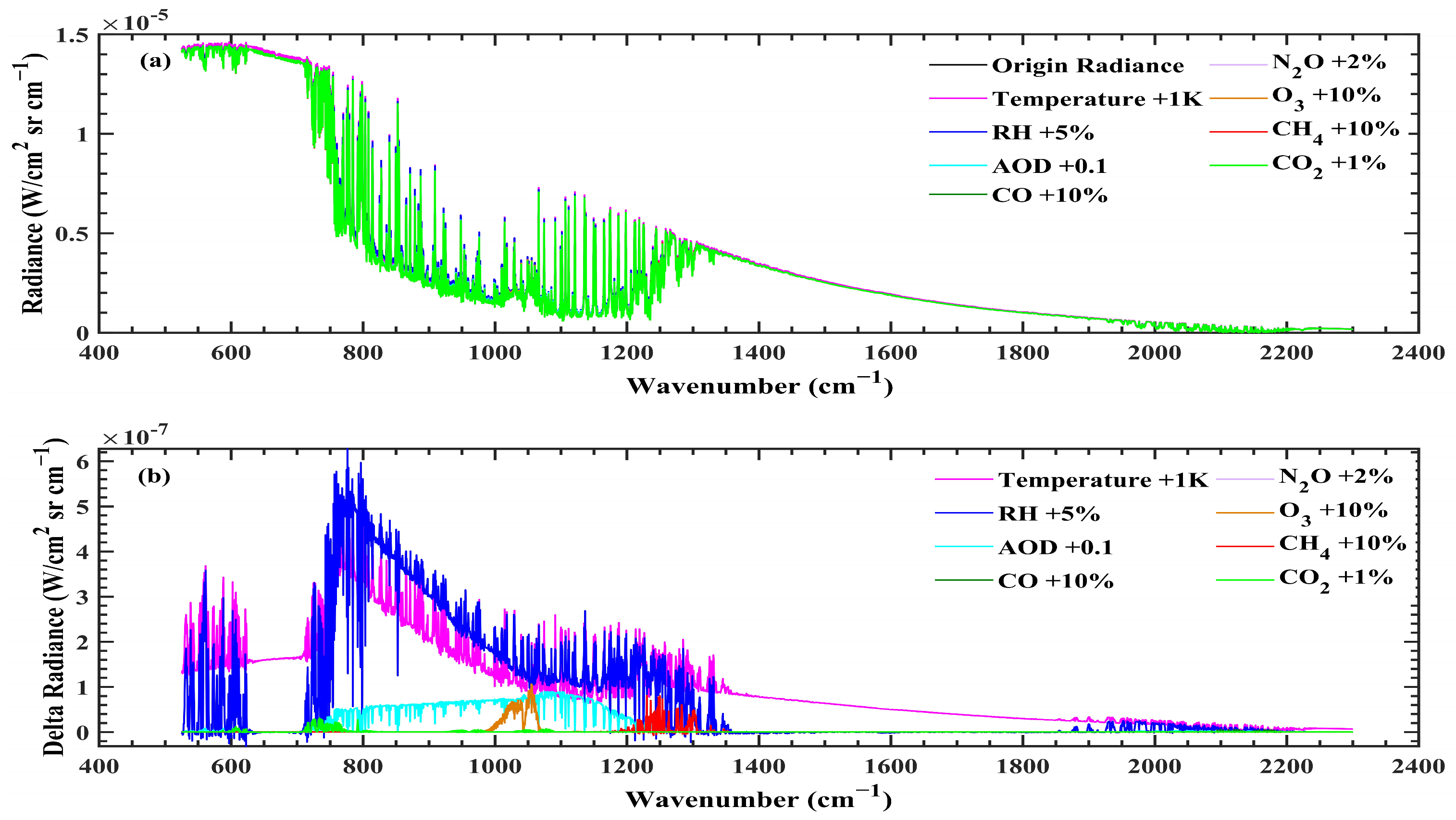
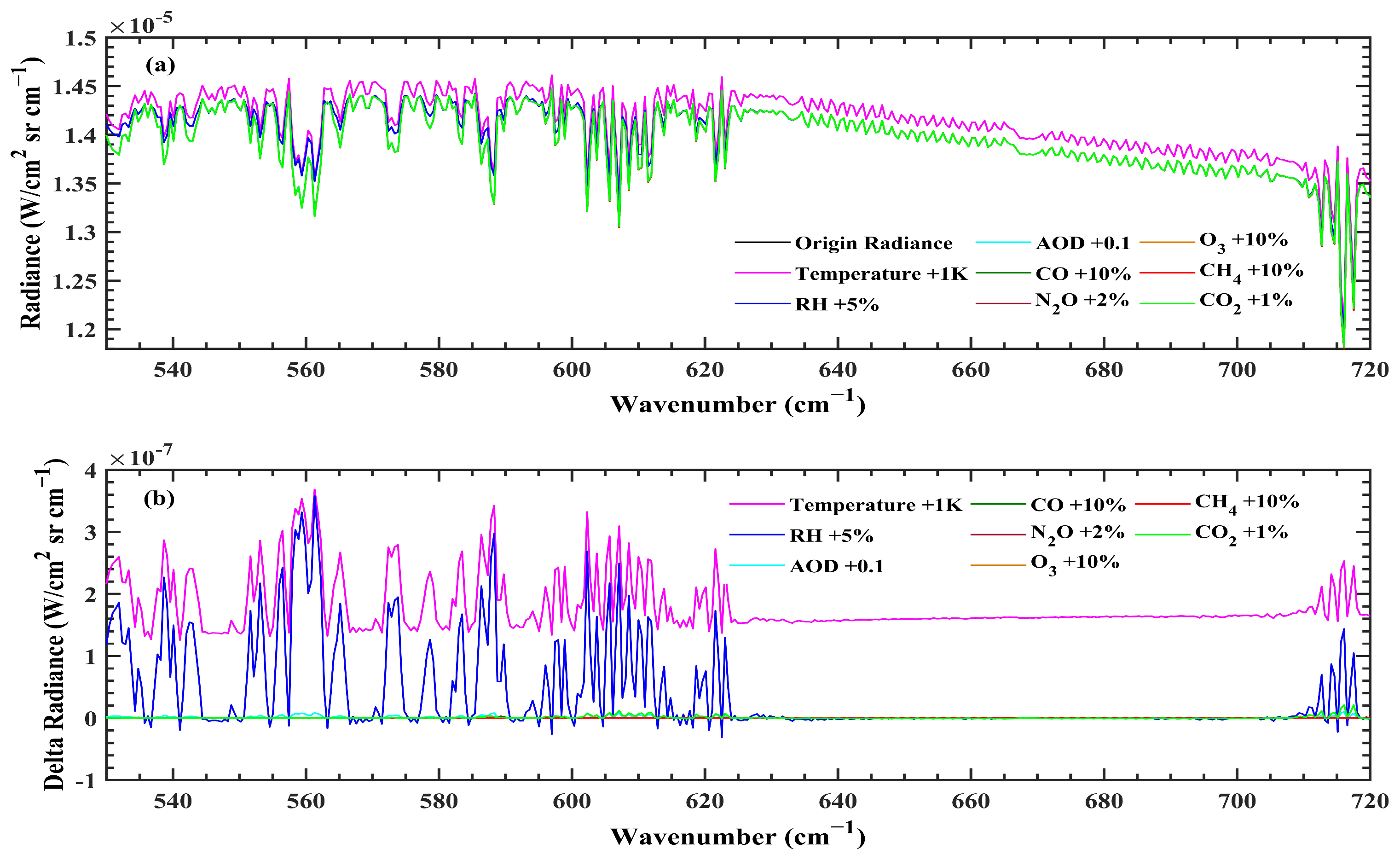
4.1. Sensitivity Test

The state of the atmosphere can have a significant impact on the downwelling thermal radiation in the thermal infrared spectral region. In this paper, LBLRTM is used to simulate the spectral radiance variations caused by changes in different factors within the 525–2300 ${\mathrm{c}\mathrm{m}}^{-1}$ range under clear-sky conditions, in order to study the sensitive channels of temperature and humidity profiles and its influencing factors using the ASSIST. The spectrum for the Anqing sounding station at 07:15 Beijing time on 2 November 2024, was simulated, with the specific simulation setup shown in

Table 2. Simulation parameters configuration.

Parameter	Configuration
Observation zenith angle	0$°$
Atmospheric emissivity	0.8
Observation altitude	0$–3 \mathrm{k}\mathrm{m}$
Number of atmospheric layers	29
Aerosol	Rural aerosol, AOD = 0.1
Temperature profile	ERA5
RH profile	ERA5
CO2 profile	Carbon Tracker
Other gas profiles	WACCM

. The spectrum set under these conditions is used as the initial spectrum. The temperature profiles (1 $\mathrm{K}$), humidity profiles (5$\%$), CO₂ profiles (1$\%$), N₂O profiles (2$\%$), O₃ profiles (10$\%$), CO profiles (10$\%$), and AOD (0.1) are sequentially increased to study the variations in spectral radiance.

Figure 3 shows that temperature and water vapor almost affect the entire thermal infrared region. To exclude the influence of other gases and AOD absorption, the temperature and humidity profiles are retrieved using the channels sensitive to temperature and humidity from the AERI [1,31]. The only difference is that, while the 674–713 ${\mathrm{c}\mathrm{m}}^{-1}$ channels are used by the AERI to retrieve the temperature profile, only the 674–703 ${\mathrm{c}\mathrm{m}}^{-1}$ channels are used for the ASSIST in this study to avoid interference from aerosol [22]. The channels used are listed in

Table 3. Channels for the retrieval of temperature and humidity profiles.

Temperature	RH
612–618 ${\mathrm{c}\mathrm{m}}^{-1}$	533–588 ${\mathrm{c}\mathrm{m}}^{-1}$
624–660 ${\mathrm{c}\mathrm{m}}^{-1}$
674–703 ${\mathrm{c}\mathrm{m}}^{-1}$

, with 147 channels dedicated to temperature retrieval and 114 channels allocated for humidity retrieval. Figure 4 shows that temperature affects the entire spectral baseline. Additionally, the channels sensitive to temperature are also sensitive to CO₂, as CO₂ exhibits strong absorption in these channels. To ensure the accuracy of the temperature and humidity profiles retrieval, all 261 channels of temperature and humidity were used, and the retrieval of temperature, humidity, and CO₂ was performed simultaneously.

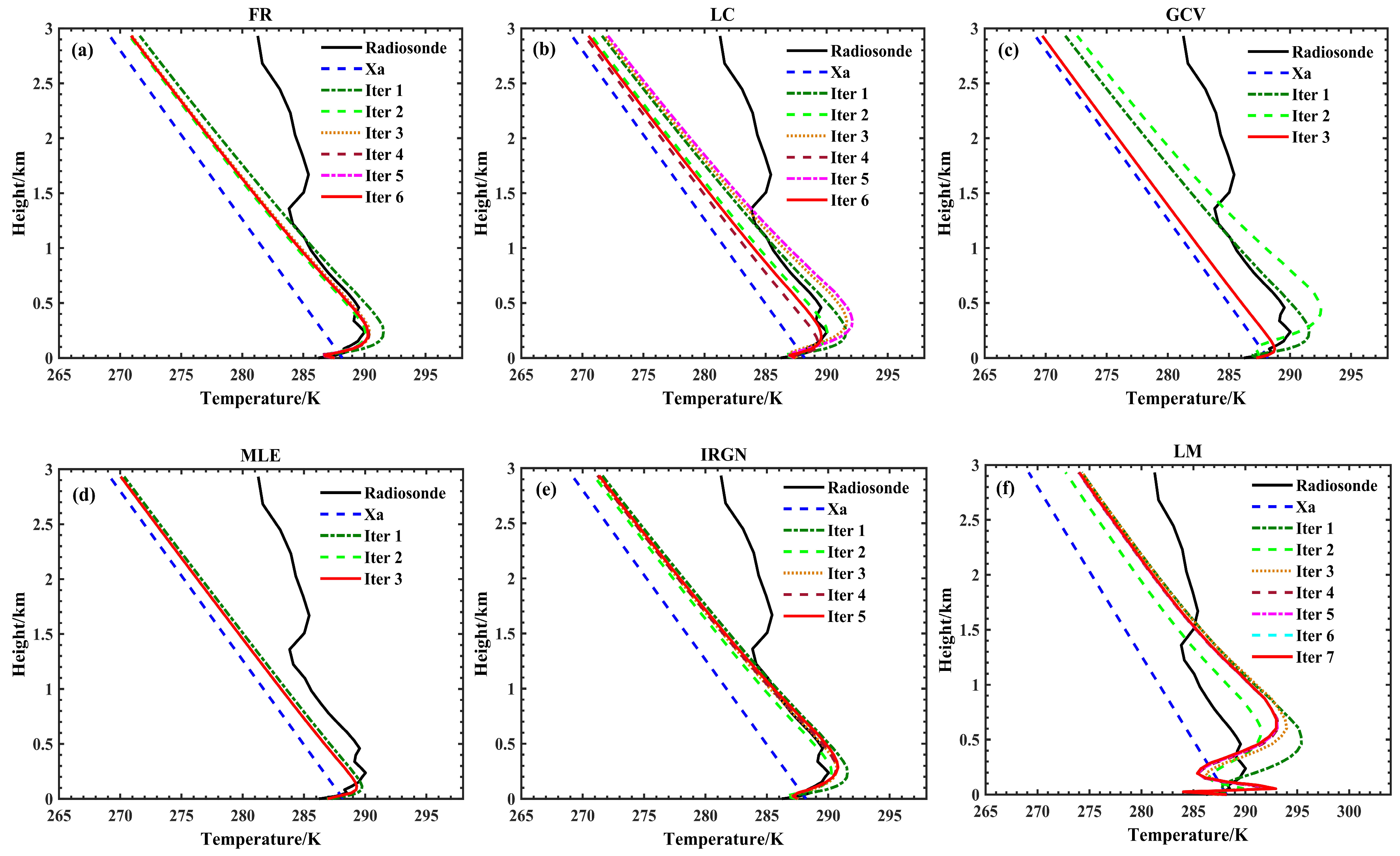
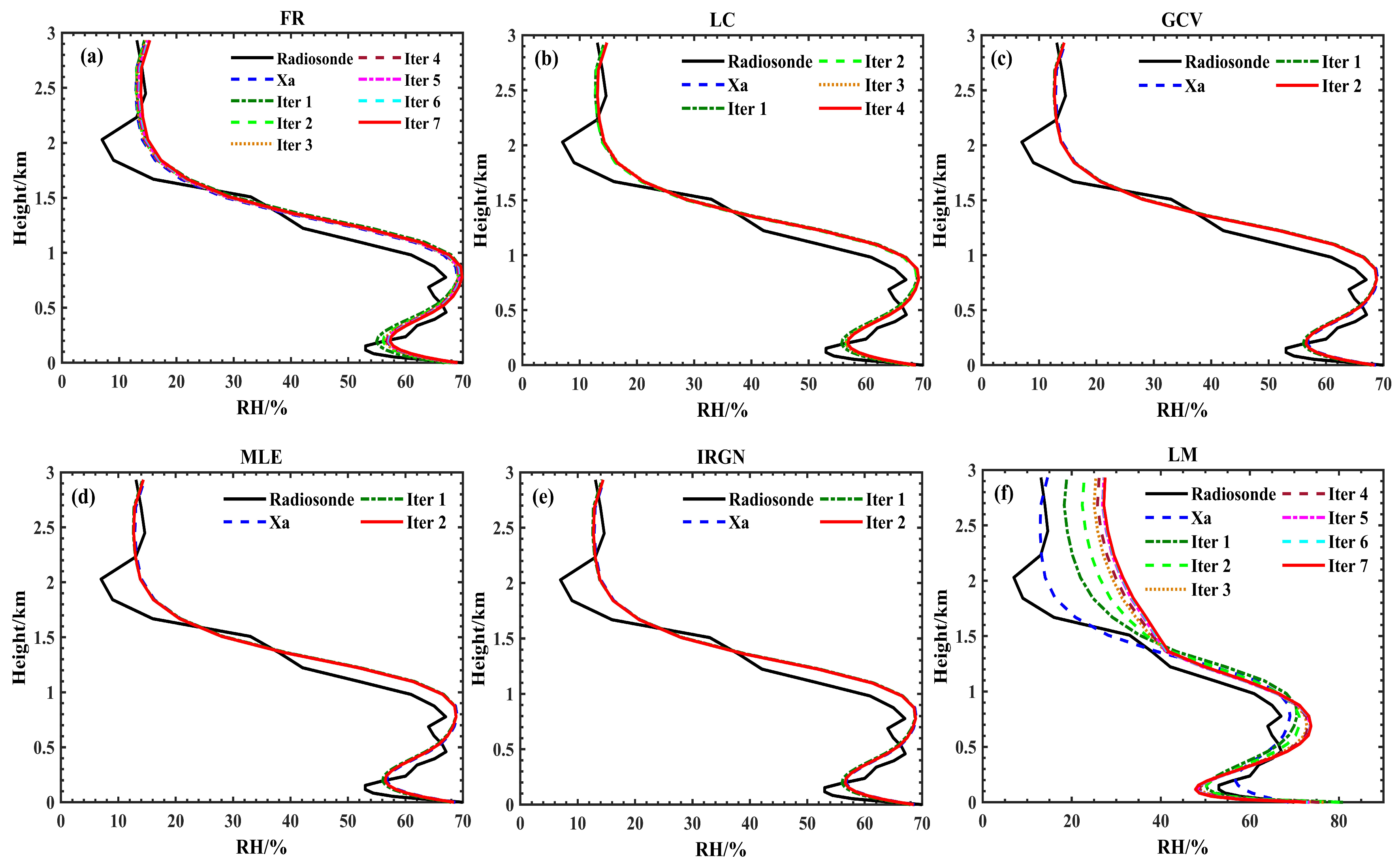
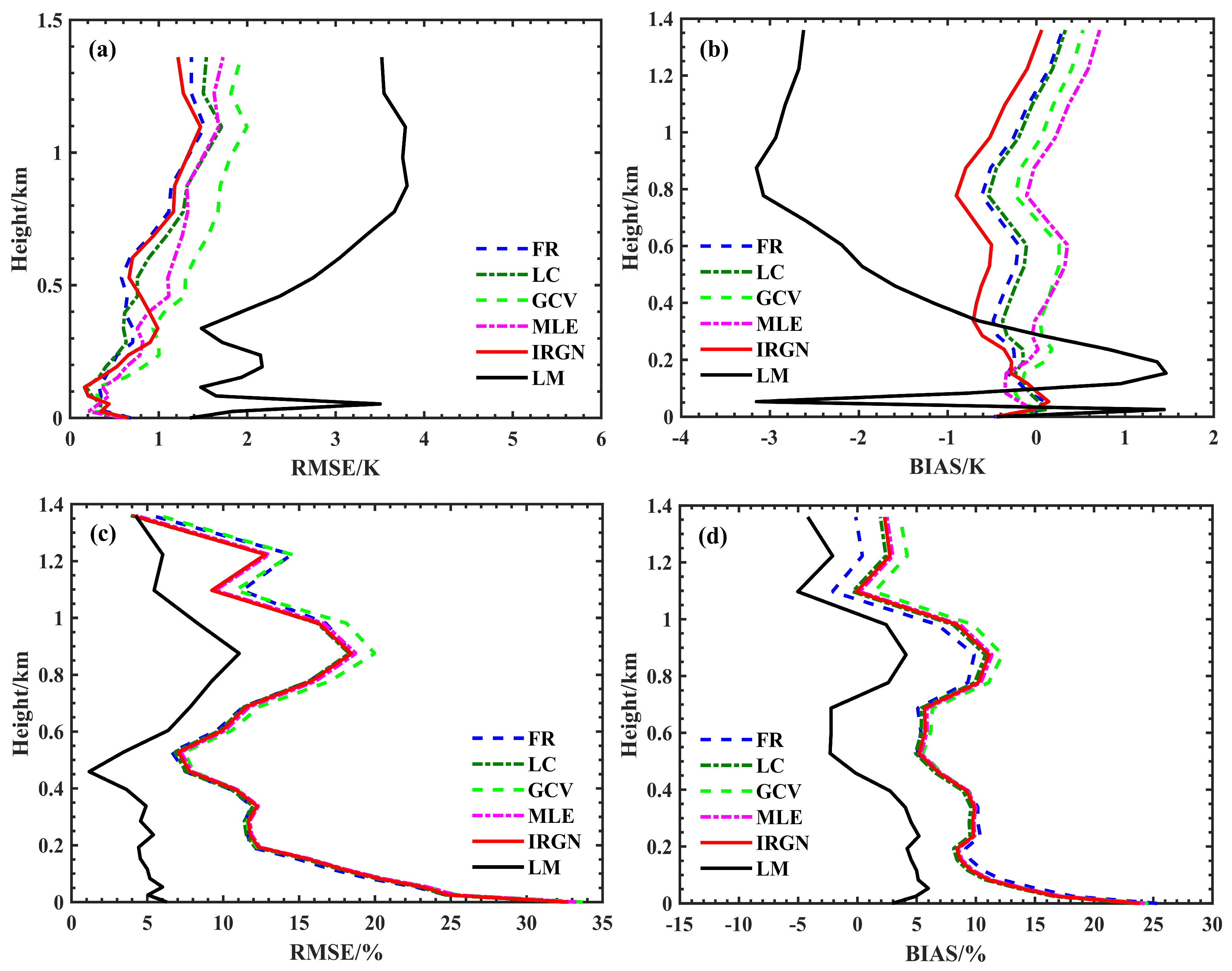
4.2. Performance of Different Regularization Methods: Case Study

To evaluate the retrieval accuracy of temperature and humidity profile using different regularization methods, the retrieval results of the measured spectra at 19:15 Beijing time on 2 November 2024, and 07:15 Beijing time on 3 November 2024, were analyzed. Since the retrieval accuracy of temperature and humidity profile is influenced by the prior profile, temperature and humidity profiles from the ERA5 dataset and the US1976 standard atmospheric model were used as prior profiles, and the retrieval was performed at different times under clear-sky conditions. Figure 5 and Figure 6 represent retrieval results using temperature profiles provided from ERA5 and US1976 standard atmospheric model as prior profiles, while Figure 7 and Figure 8 represent retrieval results using humidity profiles provided from ERA5 and US1976 standard atmospheric model as prior profiles. The retrieval results of the temperature profile in Figure 5 and Figure 6 indicate that, except for the LM method, the temperature profiles retrieved by other methods tend to converge to the prior profile above 1.5 km, leading to significant retrieval errors. This also suggests that ASSIST primarily detects temperature profile information below 1.5 km. Compared to other methods, the IRGN method demonstrates the best performance. It achieves high retrieval accuracy (see Figure 5 and Figure 6), small residual, and large DFS (see

Table 4. Comparison of the retrieval performance of temperature and humidity profiles by different methods at 19:15 Beijing time on 2 November 2024.

Date	Method	Feature	Regularization Factor	Residual $\left(\mathbf{W}/{\mathbf{c}\mathbf{m}}^2 \mathbf{s}\mathbf{r} {\mathbf{c}\mathbf{m}}^{-1}\right)$	DFS
19:15 Beijing time on 2 November 2024	FR	Temperature	$1\times {10}^4$	$2.69\times {10}^{-13}$	2.97
		RH	$1\times {10}^5$	$1.19\times {10}^{-11}$	1.43
	LC	Temperature	$1\times {10}^4$	$2.72\times {10}^{-13}$	2.97
		RH	$3\times {10}^5$	$1.64\times {10}^{-11}$	1.20
	GCV	Temperature	$1\times {10}^5$	$3.29\times {10}^{-13}$	2.18
		RH	$6\times {10}^5$	$1.34\times {10}^{-11}$	1.11
	MLE	Temperature	$1\times {10}^5$	$3.29\times {10}^{-13}$	2.18
		RH	$6\times {10}^5$	$1.34\times {10}^{-11}$	1.11
	IRGN	Temperature	$8\times {10}^3$	$1.66\times {10}^{-13}$	3.04
		RH	$4.8\times {10}^5$	$1.26\times {10}^{-11}$	1.13
	LM	Temperature	$1.25\times {10}^3$	$1.56\times {10}^{-13}$	3.74
		RH	$1.25\times {10}^4$	$4.75\times {10}^{-12}$	1.93

and

Table 5. Comparison of the retrieval performance of temperature and humidity profiles by different methods at 07:15 Beijing time on 3 November 2024.

Date	Method	Feature	Regularization Factor	Residual $\left(\mathbf{W}/{\mathbf{c}\mathbf{m}}^2 \mathbf{s}\mathbf{r} {\mathbf{c}\mathbf{m}}^{-1}\right)$	DFS
07:15 Beijing time on 3 November 2024	FR	Temperature	$1\times {10}^4$	$7.48\times {10}^{-13}$	3.00
		RH	$1\times {10}^5$	$6.81\times {10}^{-11}$	1.51
	LC	Temperature	$1\times {10}^4$	$5.55\times {10}^{-13}$	3.00
		RH	$1\times {10}^5$	$1.44\times {10}^{-11}$	1.51
	GCV	Temperature	$1\times {10}^5$	$3.15\times {10}^{-12}$	2.18
		RH	$1\times {10}^4$	$2.12\times {10}^{-10}$	2.73
	MLE	Temperature	$1\times {10}^5$	$2.07\times {10}^{-12}$	2.18
		RH	$3\times {10}^5$	$1.54\times {10}^{-10}$	1.21
	IRGN	Temperature	$4.096\times {10}^3$	$5.04\times {10}^{-13}$	3.34
		RH	$2.4576\times {10}^5$	$4.42\times {10}^{-11}$	1.25
	LM	Temperature	$1\times {10}^5$	$1.81\times {10}^{-13}$	2.18
		RH	$1\times {10}^4$	$3.97\times {10}^{-12}$	2.73

) below 1.5 km altitude, even when the initial profile deviates significantly from the true profile. This method also accurately captures the temperature inversion phenomenon in the lower atmosphere, demonstrating the algorithm’s capability to reflect fine-scale variations in temperature profile.

However, when the prior temperature profile differs significantly from the true profile, the retrieval errors of all methods increase, except for the IRGN method. Conversely, when the prior temperature profile closely resembles the true profile, all methods except for the LM method achieve high retrieval accuracy below 1.5 km altitude. When the prior temperature profile closely resembles the true profile, the GCV and MLE methods produce temperature profiles that are close to the true profile. But they also result in large residual, excessively large regularization factor, and small DFS (as shown in Table 4). The FR method and the LC method demonstrate moderate performance. The retrieval accuracy of temperature profile, residual, and DFS are all at a medium level. The LM method results in the smallest residual, but the retrieved temperature profile has largest error (see Figure 5f). This may due to overfitting caused by an excessively small spectral fitting error when using this method, resulting in high-frequency oscillation in the retrieved temperature profile. When the prior temperature profile differs significantly from the true profile, the FR and IRGN methods exhibit considerable retrieval performance, as shown in Figure 6 and Table 5.

The retrieval results of humidity profile using different methods are entirely different from those of the temperature profile. The results in Figure 7 and Figure 8 show that the humidity profiles retrieved using the first five methods exhibit only small humidity variations in each iteration and tend to converge toward the prior. This is because these methods estimate excessively large regularization factors. Figure 8 also shows that when there is a large error between the prior humidity profile and the true profile, the error of the retrieved humidity profile using the first five methods is significant. In contrast, the retrieved humidity profile using the LM method progressively approaches the true profile during iterations, even when there is a large error in the prior profile. Similarly, below 1.5 $\mathrm{k}\mathrm{m}$ altitude, the retrieval error is relatively small, but it gradually increases with altitude. Moreover, the residual from this method are an order of magnitude smaller than those from other methods, and the DFS is the largest (as shown in Table 4 and Table 5). These findings highlight the superiority of the LM method in retrieving humidity profiles using the ASSIST.

Additionally, the clear-sky spectral data collected by the ASSIST over five days (2–6 November 2024) were retrieved to evaluate the performance of different methods at various times. Figure 9 presents the RMSE and BIAS of the temperature and humidity profiles retrieved using six different methods. The results indicate that for temperature profile retrieval, the first five regularization methods produce a BIAS of less than 1 $\mathrm{K}$ and a RMSE of less than 2 $\mathrm{K}$ below 1.5 $\mathrm{k}\mathrm{m}$ altitude. However, when using the LM method, the maximum BIAS and RMSE are greater than 3 $\mathrm{K}$. For humidity profile retrieval, the BIAS and RMSE of the humidity profile obtained using the LM method are significantly lower than those of the other five regularization methods, particularly near the surface. Combining the mean residual, mean DFS, mean BIAS and RMSE below 1.5 $\mathrm{k}\mathrm{m}$ altitude as shown in

Table 6. Mean BIAS, mean RMSE, mean residual, and mean DFS of temperature and humidity profiles retrieved below 1.5 $\mathrm{k}\mathrm{m}$ altitude using different methods. The units of the mean BIAS and mean RMSE for the temperature and humidity profiles are $\mathrm{K}$ and $\%$, respectively, while the unit of the mean residual is $\left(\mathrm{W}/{\mathrm{c}\mathrm{m}}^2 \mathrm{s}\mathrm{r} {\mathrm{c}\mathrm{m}}^{-1}\right)$.

Method	Feature	Mean BIAS	Mean RMSE	Mean Residual	Mean DFS
FR	Temperature	0.29	0.77	$3.52\times {10}^{-13}$	3.14
	RH	9.10	14.57	$4.00\times {10}^{-11}$	1.47
LC	Temperature	0.23	0.82	$3.43\times {10}^{-13}$	3.27
	RH	8.74	14.40	$1.54\times {10}^{-11}$	1.36
GCV	Temperature	0.19	1.13	$8.12\times {10}^{-13}$	2.64
	RH	9.53	15.23	$1.13\times {10}^{-10}$	1.92
MLE	Temperature	0.24	0.96	$6.40\times {10}^{-13}$	2.35
	RH	9.20	14.80	$8.38\times {10}^{-11}$	1.16
IRGN	Temperature	0.42	0.80	$3.01\times {10}^{-13}$	3.37
	RH	9.01	14.58	$2.84\times {10}^{-11}$	1.19
LM	Temperature	1.80	2.60	$4.38\times {10}^{-13}$	2.93
	RH	3.65	5.62	$4.36\times {10}^{-12}$	2.05

, it can be concluded that the IRGN method achieves the best performance in retrieving the temperature profile. The mean BIAS, mean RMSE, mean residual, and mean DFS of the temperature profile are 0.42 $\mathrm{K}$, 0.80 $\mathrm{K}$, $3.01\times {10}^{-13}$ $\left(\mathrm{W}/{\mathrm{c}\mathrm{m}}^2 \mathrm{s}\mathrm{r} {\mathrm{c}\mathrm{m}}^{-1}\right)$, and 3.37, respectively. The LM method yields the poorest performance in retrieving the temperature profile. However, compared to other regularization methods, it achieves the highest accuracy in retrieving the humidity profile. The mean BIAS, mean RMSE, mean residual, and mean DFS of the humidity profile below 1.5 $\mathrm{k}\mathrm{m}$ altitude are 3.65$\%$, 5.62$\%$, $4.36\times {10}^{-12}$ $\left(\mathrm{W}/{\mathrm{c}\mathrm{m}}^2 \mathrm{s}\mathrm{r} {\mathrm{c}\mathrm{m}}^{-1}\right)$, and 2.05, respectively. In comparison, the mean BIAS, mean RMSE, and mean residual of the retrieved humidity profiles using other regularization methods are all large. This is because the prior humidity profile differs significantly from the true humidity profile, and the excessively large regularization factor causes the retrieved humidity profile to closely resemble the prior profile.

5. Conclusions and Discussion

The systematic evaluation of regularization methods and the LM algorithm for the retrieval of temperature and humidity profile using the ASSIST reveals distinct performance under actual atmospheric conditions. For temperature retrieval, the IRGN method demonstrates superior performance, even when there is a large error in the prior profile, particularly below 1.5 $\mathrm{k}\mathrm{m}$ altitude, achieving a mean BIAS of 0.42 $\mathrm{K}$, a mean RMSE of 0.80 $\mathrm{K}$, a high DFS of 3.37 and a mean residual of $3.01\times {10}^{-13}$ $\left(\mathrm{W}/{\mathrm{c}\mathrm{m}}^2 \mathrm{s}\mathrm{r} {\mathrm{c}\mathrm{m}}^{-1}\right)$. Different from traditional regularization methods, the IRGN method avoids explicit regularization factor optimization in each iteration, which reduces the computational cost while maintaining the accuracy. The accuracy of the prior profile greatly impacts the temperature profile retrieval accuracy of the five methods, except for the IRGN method. The greater the difference between the prior temperature profile and the true profile, the lower the retrieval accuracy of the profile. In contrast, the LM method, despite yielding the smallest residual, introduces high-frequency oscillation, leading to significant error (maximum BIAS and RMSE over 3 $\mathrm{K}$ below 1.5 $\mathrm{k}\mathrm{m}$ altitude), indicating overfitting. Meanwhile, when the prior temperature profile closely resembles the true profile, the methods such as GCV and MLE, though producing temperature profiles closest to the true state, suffer from excessive regularization, leading to degraded DFS and large residuals.

For humidity retrieval, the LM method outperforms all regularization-based approaches, achieving the lowest mean BIAS (3.65$\%$), mean RMSE (5.62$\%$), the lowest mean residual ($4.36\times {10}^{-12}$ $\left(\mathrm{W}/{\mathrm{c}\mathrm{m}}^2 \mathrm{s}\mathrm{r} {\mathrm{c}\mathrm{m}}^{-1}\right)$) and the highest DFS (2.05) below 1.5 $\mathrm{k}\mathrm{m}$ altitude. Its iterative damping mechanism effectively balances spectral fitting accuracy and physical plausibility, even with imperfect prior estimates. Conversely, the traditional regularization methods such as GCV, LC, MLE and FR exhibit strong prior dependence, causing retrievals to converge toward the initial guess. However, when the initial guess has a large error, it leads to significant retrieval errors. These findings suggest that the IRGN method is the preferred choice for temperature profile retrieval due to its balance of accuracy, computational efficiency, and robustness, while the LM method is recommended for humidity profile retrieval, especially in scenarios with significant prior uncertainty.

This study only evaluates the retrieval accuracy of temperature and humidity profiles using different methods under clear sky conditions for the ASSIST. Future work will extend this evaluation to cloudy and polluted conditions and explore hybrid retrieval strategies that combine a physical model (such as the atmospheric radiative transfer model) with machine learning to enhance operational meteorological applications.

References

1. Huang, W.; Liu, L.; Yang, B.; Hu, S.; Yang, W.; Li, Z.; Li, W.; Yang, X. Retrieval of temperature and humidity profiles from ground-based high-resolution infrared observations using an adaptive fast iterative algorithm. Atmos. Meas. Tech. 2023, 16, 4101–4114. [Google Scholar] [CrossRef]
2. Li, J.; Wang, P.; Han, H.; Li, J.; Zheng, J. On the assimilation of satellite sounder data in cloudy skies in numerical weather prediction models. J. Meteorol. Res. 2016, 30, 169–182. [Google Scholar] [CrossRef]
3. Wulfmeyer, V.; Hardesty, R.M.; Turner, D.D.; Behrendt, A.; Cadeddu, M.P.; Di Girolamo, P.; Schlüssel, P.; Van Baelen, J.; Zus, F. A review of the remote sensing of lower tropospheric thermodynamic profiles and its indispensable role for the understanding and the simulation of water and energy cycles. Rev. Geophys. 2015, 53, 819–895. [Google Scholar] [CrossRef]
4. Romine, G.S.; Schwartz, C.S.; Snyder, C.; Anderson, J.L.; Weisman, M.L. Model bias in a continuously cycled assimilation system and its influence on convection-permitting forecasts. Mon. Weather Rev. 2013, 141, 1263–1284. [Google Scholar] [CrossRef]
5. Yang, W.; Liu, L.; Deng, W.; Huang, W.; Ye, J.; Hu, S. Deep retrieval architecture of temperature and humidity profiles from ground-based infrared hyperspectral spectrometer. Remote Sens. 2023, 15, 2320. [Google Scholar] [CrossRef]
6. Gonzalez, L.; Kos, L.; Lavas, S.; Douglas, M. A new possible plan for a more cost-effective adaptive radiosonde observing strategy for the United States. J. Atmos. Ocean. Technol. 2012, 29, 1–25. [Google Scholar]
7. Chu, Y.; Wang, Z.; Xue, L.; Deng, M.; Lin, G.; Xie, H.; Shin, H.H.; Li, W.; Firl, G.; D’Amico, D.F. Characterizing warm atmospheric boundary layer over land by combining Raman and Doppler lidar measurements. Opt. Express 2022, 30, 11892–11911. [Google Scholar] [CrossRef]
8. Mao, J.; Abshire, J.B.; Kawa, S.R.; Sun, X.; Riris, H. Airborne lidar measurements of atmospheric CO2 column concentrations to cloud tops made during the 2017 ASCENDS/ABoVE campaign. Atmos. Meas. Tech. 2023, 17, 1–26. [Google Scholar] [CrossRef]
9. Yang, F.; Gao, F.; Zhang, C.; Li, X.; Gao, X.; Hua, D.; Wang, L.; Xin, W.; Stanič, S. Lateral scanning Raman scattering lidar for accurate measurement of atmospheric temperature and water vapor from ground to height of interest. Opt. Lett. 2023, 48, 2595–2598. [Google Scholar] [CrossRef]
10. Liu, F.; Wang, R.; Yi, F.; Huang, W.; Ban, C.; Pan, W.; Wang, Z.; Hu, H. Pure rotational Raman lidar for full-day troposphere temperature measurement at Zhongshan Station (69.37° S, 76.37° E), Antarctica. Opt. Express 2021, 29, 10059–10076. [Google Scholar] [CrossRef]
11. Schneider, M.; Hase, F.; Blumenstock, T. Water vapour profiles by ground-based FTIR spectroscopy: Study for an optimised retrieval and its validation. Atmos. Chem. Phys. 2006, 6, 811–830. [Google Scholar] [CrossRef]
12. Angelbratt, J.; Mellqvist, J.; Blumenstock, T.; Borsdorff, T.; Brohede, S.; Duchatelet, P.; Forster, F.; Hase, F.; Mahieu, E.; Murtagh, D. A new method to detect long-term trends of methane (CH4) and nitrous oxide (N2O) total columns measured within the NDACC ground-based high-resolution solar FTIR network. Atmos. Chem. Phys. 2011, 11, 6167–6183. [Google Scholar] [CrossRef]
13. De Mazière, M.; Thompson, A.M.; Kurylo, M.J.; Wild, J.D.; Bernhard, G.; Blumenstock, T.; Braathen, G.O.; Hannigan, J.W.; Lambert, J.C.; Leblanc, T. The Network for the Detection of Atmospheric Composition Change (NDACC): History, status and perspectives. Atmos. Chem. Phys. 2018, 18, 4935–4964. [Google Scholar] [CrossRef]
14. Knuteson, R.; Revercomb, H.; Best, F.; Ciganovich, N.; Dedecker, R.; Dirkx, T.; Ellington, S.; Feltz, W.; Garcia, R.; Howell, H. Atmospheric emitted radiance interferometer. Part I: Instrument design. J. Atmos. Ocean. Technol. 2004, 21, 1763–1776. [Google Scholar] [CrossRef]
15. Rochette, L.; Smith, W.L.; Howard, M.; Bratcher, T. In ASSIST, Atmospheric Sounder Spectrometer for Infrared Spectral Technology: Latest development and improvement in the atmospheric sounding technology. In Imaging Spectrometry XIV; SPIE: Bellingham, WA, USA, 2009; pp. 9–17. [Google Scholar]
16. Michaud-Belleau, V.; Gaudreau, M.; Lacoursière, J.; Boisvert, É.; Ravelomanantsoa, L.; Turner, D.D.; Rochette, L. The Atmospheric Sounder Spectrometer by Infrared Spectral Technology (ASSIST): Instrument design and signal processing. EGUsphere 2025, 2025, 1–39. [Google Scholar]
17. Schneider, M.; Hase, F. Ground-based FTIR water vapour profile analyses. Atmos. Meas. Tech. 2009, 2, 609–619. [Google Scholar] [CrossRef]
18. Barthlott, S.; Schneider, M.; Hase, F.; Blumenstock, T.; Kiel, M.; Dubravica, D.; García, O.E.; Sepúlveda, E.; Mengistu Tsidu, G.; Takele Kenea, S. Tropospheric water vapour isotopologue data (H216O, H218O, and HD16O) as obtained from NDACC/FTIR solar absorption spectra. Earth Syst. Sci. Data 2017, 9, 15–29. [Google Scholar] [CrossRef]
19. Turner, D.; Löhnert, U. Information content and uncertainties in thermodynamic profiles and liquid cloud properties retrieved from the ground-based Atmospheric Emitted Radiance Interferometer (AERI). J. Appl. Meteorol. Climatol. 2014, 53, 752–771. [Google Scholar] [CrossRef]
20. Yurganov, L.; McMillan, W.; Wilson, C.; Fischer, M.; Biraud, S.; Sweeney, C. Carbon monoxide mixing ratios over Oklahoma between 2002 and 2009 retrieved from Atmospheric Emitted Radiance Interferometer spectra. Atmos. Meas. Tech. 2010, 3, 1319–1331. [Google Scholar] [CrossRef]
21. Seo, J.; Choi, H.; Oh, Y. Potential of AOD retrieval using atmospheric emitted radiance interferometer (AERI). Remote Sens. 2022, 14, 407. [Google Scholar] [CrossRef]
22. Wang, Y.; Ye, H.; Shi, H.; Wang, X.; Li, C.; Sun, E.; An, Y.; Wu, S.; Xiong, W. Channel selection method for the CH4 profile retrieval using the Atmospheric Sounder Spectrometer by Infrared Spectral Technology. J. Quant. Spectrosc. Radiat. Transf. 2024, 326, 109118. [Google Scholar] [CrossRef]
23. Yang, J.; Min, Q. Retrieval of atmospheric profiles in the New York State Mesonet using one-dimensional variational algorithm. J. Geophys. Res. Atmos. 2018, 123, 7563–7575. [Google Scholar] [CrossRef]
24. Milstein, A.B.; Santanello, J.A.; Blackwell, W.J. Detail enhancement of AIRS/AMSU temperature and moisture profiles using a 3D deep neural network. Artif. Intell. Earth Syst. 2023, 2, 1–31. [Google Scholar] [CrossRef]
25. Bouillon, M.; Safieddine, S.; Whitburn, S.; Clarisse, L.; Aires, F.; Pellet, V.; Lezeaux, O.; Scott, N.A.; Doutriaux-Boucher, M.; Clerbaux, C. Time evolution of temperature profiles retrieved from 13 years of infrared atmospheric sounding interferometer (IASI) data using an artificial neural network. Atmos. Meas. Tech. 2022, 15, 1779–1793. [Google Scholar] [CrossRef]
26. Luo, Y.; Wu, H.; Gu, T.; Wang, Z.; Yue, H.; Wu, G.; Zhu, L.; Pu, D.; Tang, P.; Jiang, M. Machine learning model-based retrieval of temperature and relative humidity profiles measured by microwave radiometer. Remote Sens. 2023, 15, 3838. [Google Scholar] [CrossRef]
27. Zanetta, F.; Nerini, D.; Beucler, T.; Liniger, M.A. Physics-constrained deep learning postprocessing of temperature and humidity. Artif. Intell. Earth Syst. 2023, 2, e220089. [Google Scholar] [CrossRef]
28. Liu, Q.; Liang, X. Physics-constrained deep learning-based radiative transfer model. Opt. Express 2023, 31, 28596–28610. [Google Scholar] [CrossRef]
29. Xu, J.; Schreier, F.; Doicu, A.; Trautmann, T. Assessment of Tikhonov-type regularization methods for solving atmospheric inverse problems. J. Quant. Spectrosc. Radiat. Transf. 2016, 184, 274–286. [Google Scholar] [CrossRef]
30. Li, J.; Huang, H.L. Retrieval of atmospheric profiles from satellite sounder measurements by use of the discrepancy principle. Appl. Opt. 1999, 38, 916–923. [Google Scholar] [CrossRef]
31. Turner, D.D.; Blumberg, W.G. Improvements to the AERIoe thermodynamic profile retrieval algorithm. IEEE J. Sel. Top. Appl. Earth Obs. Remote Sens. 2018, 12, 1339–1354. [Google Scholar] [CrossRef]
32. Hansen, P.C. Analysis of discrete ill-posed problems by means of the L-curve. SIAM Rev. 1992, 34, 561–580. [Google Scholar] [CrossRef]
33. Fuhry, M.; Reichel, L. A new Tikhonov regularization method. Numer. Algorithms 2012, 59, 433–445. [Google Scholar] [CrossRef]
34. Wahba, G. Practical approximate solutions to linear operator equations when the data are noisy. SIAM J. Numer. Anal. 1977, 14, 651–667. [Google Scholar] [CrossRef]
35. Demoment, G. Image reconstruction and restoration: Overview of common estimation structures and problems. IEEE Trans. Acoust. Speech Signal Process. 1989, 37, 2024–2036. [Google Scholar] [CrossRef]
36. Hansen, P.C. The L-curve and its use in the numerical treatment of inverse problems. Comput. Inverse Probl. Electrocardiol. 2001, 4, 119–142. [Google Scholar]
37. Eriksson, P. Analysis and comparison of two linear regularization methods for passive atmospheric observations. J. Geophys. Res. Atmos. 2000, 105, 18157–18167. [Google Scholar] [CrossRef]
38. Rodgers, C.D. Inverse Methods for Atmospheric Sounding: Theory and Practice; World Scientific: Singapore, 2000; p. 238. [Google Scholar]
39. Liu, X.; Zhou, D.K.; Larar, A.M.; Smith, W.L.; Schluessel, P.; Newman, S.M.; Taylor, J.P.; Wu, W. Retrieval of atmospheric profiles and cloud properties from IASI spectra using super-channels. Atmos. Chem. Phys. 2009, 9, 9121–9142. [Google Scholar] [CrossRef]
40. Gamage, S.M.; Sica, R.J.; Martucci, G.; Haefele, A. A 1D Var retrieval of relative humidity using the ERA5 dataset for the assimilation of Raman lidar measurements. J. Atmos. Ocean. Technol. 2020, 37, 2051–2064. [Google Scholar] [CrossRef]
41. Panditharatne, S.; Brindley, H.; Cox, C.; Siddans, R.; Murray, J.; Warwick, L.; Fox, S. Retrievals of water vapour and temperature exploiting the far-infrared: Application to aircraft observations in preparation for the FORUM mission. Atmos. Meas. Tech. 2025, 18, 717–735. [Google Scholar] [CrossRef]
42. Peter, D.; Heinz, W.E.; Otmar, S. A convergence analysis of iterative methods for the solution of nonlinear ill-posed problems under affinely invariant conditions. Inverse Probl. 1998, 14, 1081. [Google Scholar]
43. Doicu, A.; Schreier, F.; Hess, M. Iteratively regularized Gauss–Newton method for atmospheric remote sensing. Comput. Phys. Commun. 2002, 148, 214–226. [Google Scholar] [CrossRef]
44. Doicu, A.; Schreier, F.; Hess, M. Iterative regularization methods for atmospheric remote sensing. J. Quant. Spectrosc. Radiat. Transf. 2004, 83, 47–61. [Google Scholar] [CrossRef]
45. Smith, W.L., Sr.; Weisz, E.; Kireev, S.V.; Zhou, D.K.; Li, Z.; Borbas, E.E. Dual-regression retrieval algorithm for real-time processing of satellite ultraspectral radiances. J. Appl. Meteorol. Climatol. 2012, 51, 1455–1476. [Google Scholar] [CrossRef]
46. Durre, I.; Yin, X.; Vose, R.S.; Applequist, S.; Arnfield, J. Enhancing the data coverage in the Integrated Global Radiosonde Archive. J. Atmos. Ocean. Technol. 2018, 35, 1753–1770. [Google Scholar] [CrossRef]
47. Chen, Z.; Gao, J.; Yang, X. Introduction of IGRA dataset and analysis of its data quality. J. Meteorol. Environ. 2013, 29, 106–111. [Google Scholar]
48. Twomey, S. On the Numerical Solution of Fredholm Integral Equations of the First Kind by the Inversion of the Linear System Produced by Quadrature. J. ACM 1963, 10, 97–101. [Google Scholar] [CrossRef]
49. Choudhury, D.; Ji, F.; Nishant, N.; Di Virgilio, G. Evaluation of ERA5-simulated temperature and its extremes for Australia. Atmosphere 2023, 14, 913. [Google Scholar] [CrossRef]
50. Mustafa, F.; Wang, H.; Bu, L.; Wang, Q.; Shahzaman, M.; Bilal, M.; Zhou, M.; Iqbal, R.; Aslam, R.W.; Ali, M.A. Validation of GOSAT and OCO-2 against in situ aircraft measurements and comparison with carbontracker and GEOS-CHEM over Qinhuangdao, China. Remote Sens. 2021, 13, 899. [Google Scholar] [CrossRef]
51. Garcia, R.R.; López-Puertas, M.; Funke, B.; Marsh, D.R.; Kinnison, D.E.; Smith, A.K.; González-Galindo, F. On the distribution of CO2 and CO in the mesosphere and lower thermosphere. J. Geophys. Res. Atmos. 2014, 119, 5700–5718. [Google Scholar] [CrossRef]
52. Eguchi, N.; Saito, R.; Saeki, T.; Nakatsuka, Y.; Belikov, D.; Maksyutov, S. A priori covariance estimation for CO2 and CH4 retrievals. J. Geophys. Res. Atmos. 2010, 115, D10215. [Google Scholar] [CrossRef]
Figure 1. The location of Anqing sounding site, where the ASSIST was installed.
Remotesensing 17 01440 g001
Figure 2. Spectrum measured by the ASSIST under a clear sky at 07:16:44 Beijing time (UTC + 8) on 3 November 2024.
Remotesensing 17 01440 g002
Figure 3. Simulated radiance and the radiance changes resulting from variations in a single element within the 525–2300 c m 1 band. (a) represents the original and changed spectral radiance. (b) represents the differences in spectral radiance.
Remotesensing 17 01440 g003
Figure 4. Simulated radiance and the radiance changes resulting from variations in a single element within the 530–720 c m 1 band. (a) represents the original and changed spectral radiance. (b) represents the differences in spectral radiance.
Remotesensing 17 01440 g004
Figure 5. Results of temperature profile retrieval using different methods at 19:15 Beijing Time on 2 November 2024. X a in the figure represents the prior temperature profile, derived from ERA5 data interpolated to the retrieval height. The iteration number represents the iteration at which the retrieval converges. The black line represents the true profile, while the red line represents the profile when the retrieval has converged. (af) represent the results using FR, LC, GCV, MLE, IRGN, and LM methods, respectively.
Remotesensing 17 01440 g005
Figure 6. Results of temperature profile retrieval using different methods at 07:15 Beijing Time on 3 November 2024. X a in the figure represents the prior temperature profile, derived from the US1976 standard atmospheric model data interpolated to the retrieval height. Similarly, the iteration number represents the iteration at which the retrieval converges. The black line represents the true profile, while the red line represents the profile when the retrieval has converged. (af) represent the results using FR, LC, GCV, MLE, IRGN, and LM methods, respectively.
Remotesensing 17 01440 g006
Figure 7. Results of humidity profile retrieval using different methods at 19:15 Beijing Time on 2 November 2024. X a in the figure represents the prior humidity profile, derived from ERA5 data interpolated to the retrieval height. The iteration number represents the iteration at which the retrieval converges. The black line represents the true profile, while the red line represents the profile when the retrieval has converged. (af) represent the results using FR, LC, GCV, MLE, IRGN, and LM methods, respectively.
Remotesensing 17 01440 g007
Figure 8. Results of humidity profile retrieval using different methods at 07:15 Beijing Time on 3 November 2024. X a in the figure represents the prior humidity profile, derived from the US1976 standard atmospheric model data interpolated to the retrieval height. Similarly, the iteration number represents the iteration at which the retrieval converges. The black line represents the true profile, while the red line represents the profile when the retrieval has converged. (af) represent the results using FR, LC, GCV, MLE, IRGN, and LM methods, respectively.
Remotesensing 17 01440 g008
Figure 9. RMSE and BIAS of temperature and humidity profiles retrieved below 1.5 k m altitude using different methods. The top row, (a,b), represents the results of temperature profile, while the bottom row, (c,d), represents the results of the humidity profile.
Remotesensing 17 01440 g009