Exploring the Causes of Severe Fluctuations in Water Surface Area Using Water Index and Structural Equation Modeling: Evidence from Ebinur Lake, China

Abstract

Arid zone lakes function as indicators of watershed ecology and environment, significantly influencing regional social development. In Ebinur Lake, a fuzzy water–land boundary hinders lake area extraction using remote sensing. Furthermore, unquantifiable anthropogenic–natural factors make it difficult to explore the drivers of lake area change. Utilizing Google Earth Engine (GEE), this study employs Landsat series, Sentinel 2, and MOD09GA/MYD09GA data to extract the water area of Ebinur Lake by applying indices such as NDWI, MNDWI, AWEI, and MAWEI. Threshold determination and shoreline refinement are achieved through Otsu’s method and the Canny algorithm, followed by a comparative analysis. Monthly spatiotemporal variations between 2009 and 2023 are analyzed using distance-level analysis and center-of-gravity analyses. It is noteworthy that this study adopted PLS-SEM. By comprehensively considering multifactorial interactions, this approach effectively simulates real-world natural scenarios and quantitatively evaluates the complex impacts of hydrology, meteorology, soil–vegetation, and human activities that influence changes in lake area. The results are as follows: (1) MAWEI outperforms NDWI, MNDWI, and AWEI with >95% overall accuracy and a Kappa coefficient >0.9, making it the best index for water body extraction; (2) from 2009 to 2017, Ebinur Lake’s area gradually increased, falling within a range of 450 km² to 900 km². Conversely, from 2017 to 2023, the lake’s area notably decreased, falling to between 330 km² and 880 km²; (3) Ebinur Lake’s center of gravity shifts northwest to southeast, with primary changes in northwest mini-lake and transition zones; (4) hydrological factors were identified as the primary driver of changes in the Ebinur Lake area, contributing 64.3% of the total impact. Soil–vegetation, human activities, and meteorological factors contributed 16.7%, 11.3%, and 7.8%, respectively. The quantified driving factors and the MAWEI-based monitoring framework can directly provide references for water resource allocation policies and ecological restoration priorities in the economic zone of the Tianshan Mountains.

1. Introduction

Lakes are vital surface water reservoirs, playing a crucial role in flood control, irrigation, tourism, and fisheries [1,2,3]. Among them, lakes in inland arid zones are particularly significant as they mirror the local climate, environmental conditions, and biological features [4]. However, in the context of climate change and intensified human activities, lakes in China’s arid and semi-arid regions are shrinking [5,6,7]. This shrinkage leads to more severe water shortages and seriously endangers human livelihoods as well as the ecological balance. Thus, understanding the spatiotemporal changes and driving mechanisms of lake areas in arid zones is highly important for sustainable development.

Ebinur Lake, Xinjiang’s premier saline lake, constitutes a pivotal ecological barrier in northwest China [8]. It is a typical inland lake in the arid zone [9], which has the role of maintaining the water balance and ecological security of the surface water. With the development of the economic zone on the north slope of Tianshan Mountain, the water resources of Ebinur Lake are seriously threatened. Its watershed ecological environment is also becoming increasingly fragile, posing a threat to the sustainable development of the economic zone [10]. Since the 1950s, the Kuytun River has ceased to flow into Ebinur Lake following the construction of upstream reservoirs [11,12]. Additionally, the surface area of Ebinur Lake has exhibited natural fluctuations since the last century, yet intensive anthropogenic disturbances over the past four decades have precipitated severe ecological degradation in the region [13,14]. Currently, Ebinur Lake has become a primary source of dust storms and airborne pollutants in northern Xinjiang, exacerbating local environmental pressures and impeding socioeconomic development. Continuous monitoring of the surface water dynamics of Ebinur Lake is now indispensable for identifying the drivers of fluctuations in its size, assessing long-term trends, and formulating sustainable water resource management strategies and ecological restoration policies.

Since the 1970s, the proliferation of remote-sensing technology has significantly broadened its utilization in unraveling the intricate dynamics of lakes across diverse scales. This technology offers a potent tool for acquiring extensive temporal series and spatially diverse characterizations of lake transformations [15]. The most widely used water body extraction methods in optical remote-sensing images are the traditional Manual Visual Interpretation Method, Thresholding Method, and Classification Method [16], among which the Thresholding Method can be categorized into the Single-Band Thresholding Method [17], Interspectral Relationship Method [18] and the Water Body Index Method [19]. The Water Body Index Method was originally proposed by Ouma et al. [20], while McFeeters [21] created the NDWI (Normalized Difference Water Index), as the Interspectral Relationship Method was too complex and the associated analytical process was not effective in suppressing background information. With the depth of research and application, scholars have proposed targeted water body extraction models for the characteristics of different regional water systems. For example, Xu [22] proposed the MNDWI (Modified Normalized Difference Water Index) for urban regional water body extraction; Feyisa et al. [23] proposed the AWEI (Automated Water Extraction Index), an automatic water body extraction index capable of extracting high-precision water bodies, based on the MNDWI, which is advantageous in mountainous areas with large mountain shadows; and Wang et al. [24] employed the MAWEI (Modified Automated Water Extraction Index) to extract the water body area, aiming to invert the concentration of suspended particulate matter in turbid water. Zhou et al. [25] extracted the water areas of Poyang Lake by using the NDWI based on 22 periods of high-resolution images, and they analyzed the changes in the time series of the water surface. Moknatian et al. [26] used the spatial segmentation and thresholding techniques to remove clouds and associated shadows in the scene, and then they extracted the water bodies using water body indexes. Achary et al. [17] proposed two water body indexes, the NDWI and AWEI_sh (Automated Water Extraction Index), combined with the Normalized Vegetation Index (NDVI) for water body index extraction and enhanced surface water monitoring using elevation segmentation. Chen et al. [27] conducted an analysis of the spatial and temporal alterations of East Lake in Wuhan across a twenty-year span, drawing upon topographical maps and remotely sensed imagery. While remote sensing offers crucial data on the spatiotemporal variations in lakes, clarifying the root driving forces demands the incorporation of multi-source environmental datasets and advanced statistical frameworks that are proficient in deciphering the complex interplays between natural and human activities.

The literature shows that scholars have conducted studies of the driving mechanisms of lake area change [28,29]. In terms of driving mechanism research methods, these mainly have consisted of factor analysis, regression analysis [30], correlation analysis [31], trend analysis [32], gray correlation analysis [33], and model fitting and evaluation [34]. The first five methods are known for their simplicity, accessibility, and wide applicability, and they are usually used in idealized situations. These methods assume a linear relationship between variables and adopt simplifying assumptions that do not fully reflect the intricacies of real-world situations. In contrast, model fitting and evaluation are more flexible, but explaining the relationship between variables is difficult. To address the limitations of traditional methods in dealing with complex variable relationships, Structural Equation Modeling (SEM) can more accurately reflect real-world processes by integrating multiple driving factors and their interactions [35,36]. Given that Partial Least Squares Structural Equation Modeling (PLS-SEM) has the ability to deal with small sample sizes and non-normal data distributions common in arid regions, to integrate various related observed variables into a unified latent structure to avoid the one-sidedness of single-factor explanations, and to clearly quantify the direct influences and indirect pathways among the factors, PLS-SEM was selected as an analytical tool in this study. In PLS-SEM analysis, model fitting begins with the creation of an initial model based on data characteristics. In evaluating models, we primarily rely on the Variance Inflation Factor (VIF), the Determination Coefficient (R²), and Predictive Relevance (Q²) [37,38]. The VIF is employed to check for linear dependencies among predictors, R² is indicative of the model’s improved goodness of fit, and a positive Q² value signifies a trustworthy prediction framework. The study area primarily includes the Qinghai-Tibet Plateau lake region, Northeast China lake region [39], and middle and lower reaches of the Yangtze River lake region [27]. Due to the scarcity of information, there are fewer studies on lake area drivers in the arid zone. Therefore, in this study, we chose a typical arid zone as the research object to explore the driving forces behind changes in lake surface area in a data-scarce region.

This study relies on the GEE platform, based on Landsat series, Sentinel 2, and MOD09GA/MYD09GA data, to carry out research on the extraction of the water body area of Ebinur Lake and the analysis of the mechanisms driving change. The primary goal of this research was to tackle the following questions: (1) Identify the optimal water body index tailored to the distinctive aquatic environment of Ebinur Lake. (2) Examine the spatial and temporal trends in the monthly shifts of Ebinur Lake’s water body spanning the past fifteen years. (3) Ascertain the key factors regulating the changes in the water body area of Ebinur Lake. The forecasted findings of this study are poised to provide practical insights for the development, utilization, and allocation of water resources within the Ebinur Lake region.

2. Materials and Methods

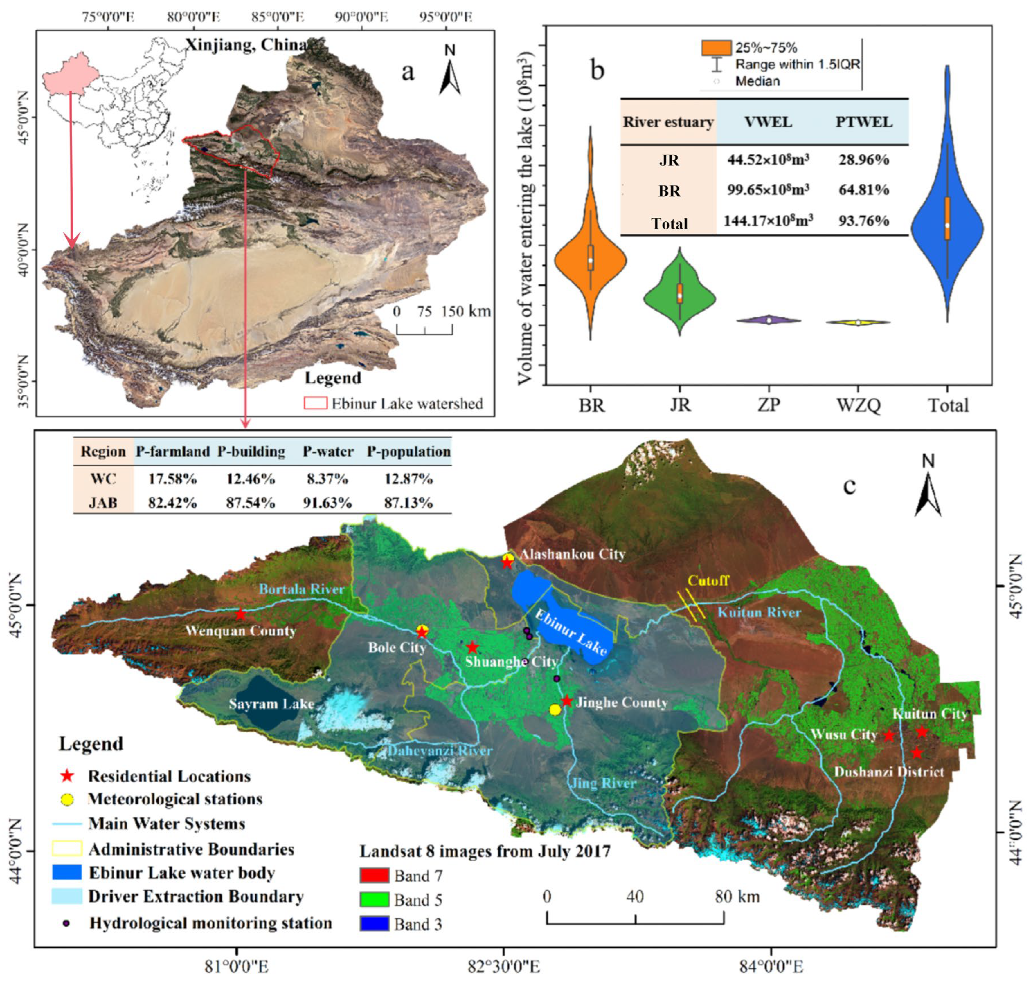
2.1. Study Area

The study is centered on Ebinur Lake on the northern slope of the Tianshan Economic Zone. The lake is located in the southwestern part of the Junggar Basin and has a flat bottom with an average depth of 1.2 m and an elevation of about 189 m [38]. The region has a temperate continental climate with a mean annual temperature of 7.8 °C, a frost-free period of 190 days, about 105 mm of annual precipitation, and about 1315 mm of annual evaporation [40,41]. Alashankou Pass is a windy pass in the northwestern part of the lake, with 164 windy days per year and maximum wind speeds up to 55.0 m/s [42]. Ebinur Lake is fed by the Jinghe and Bortala Rivers, and the lake area varies dramatically. Considering the dominance of Bole City, Alashankou City, Shuanghe City, and Jinghe County in terms of farmland, buildings, and population in the watershed (National Statistical Yearbook, 2011–2020), we defined this area as our study area. This choice allowed us to analyze the factors driving changes in the area of Ebinur Lake in a more focused and practical way [43,44] (Figure 1c).

2.2. Data Introduction and Preprocessing

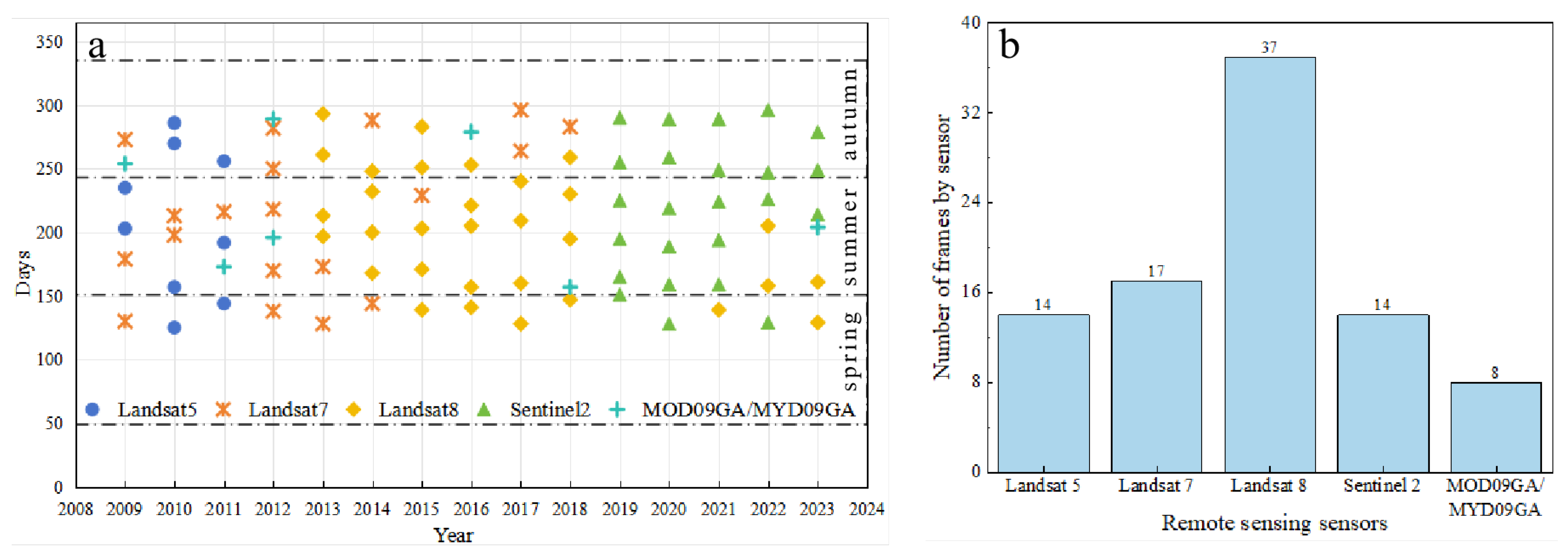
2.2.1. Remotely Sensed Data Acquisition and Preprocessing

This study started in 2009 for two reasons: First, the coverage and quality of remote-sensing data from multiple sources (e.g., Landsat, MODIS, Sentinel series) increased after that year, which provided better data for this study; second, since 2009, the promotion of water-saving irrigation, returning farmland to grassland, and other management projects has been underway, which is conducive to the assessment of the effects of ecological restoration in the past 15 years. In this study, the Level 2 data of the Landsat series and Sentinel 2 in the Ebinur Lake regional area were acquired using the GEE (https://code.earthengine.google.com/ (accessed on 6 March 2024)). Screening of images with the imaging time was carried out from May to October with less than 20% cloud cover. Missing images in the sequence of time are compensated by using MOD09GA/MYD09GA data. Note that given the inconsistency in spatial resolution of remote-sensing data in chronological order, ArcGIS 10.8 was used in this study, which resampled all the images to 30 m. The distribution of the selected 90 remote-sensing images chronologically is depicted in Figure 2.

Primarily, the spectral bands encompassing blue, green, red, near-infrared, and shortwave infrared are employed for the calculation of the water body index. The specific information regarding these bands used by the mentioned sensors is outlined in

Table 1. Remote-sensing data sources.

Image Type	Parameters	Blue	Green	Red	NIR	SWIR1	SWIR2
Landsat 5	Center wavelength (nm)	485	560	560	830	1650	2215
	Wavelength range (nm)	450–520	520–600	630–690	760–900	1550–1750	2080–2350
	Resolution (m)	30	30	30	30	30	30
	Number of bands	SR_B1	SR_B2	SR_B3	SR_B4	SR_B5	SR_B7
Landsat 7	Center wavelength (nm)	485	560	560	830	1650	2215
	Wavelength range (nm)	450–520	520–600	630–690	760–900	1550–1750	2080–2350
	Resolution (m)	30	30	30	30	30	30
	Number of bands	SR_B1	SR_B2	SR_B3	SR_B4	SR_B5	SR_B7
Landsat 8	Center wavelength (nm)	483	561	655	865	1610	2200
	Wavelength range (nm)	450–515	525–600	630–680	845–885	1560–1660	2100–2300
	Resolution (m)	30	30	30	30	30	30
	Number of bands	SR_B2	SR_B3	SR_B4	SR_B5	SR_B6	SR_B7
Sentinel 2	Center wavelength (nm)	490	560	665	842	1610	2190
	Wavelength range (nm)	458–523	543–578	650–680	789–895	1565–1655	2105–2279
	Resolution (m)	10	10	10	10	20	20
	Number of bands	B2	B3	B4	B8	B11	B12
MOD09GA/MYD09GA	Center wavelength (nm)	469	555	645	858	1640	2130
	Wavelength range (nm)	459–479	545–565	620–670	841–876	1628–1652	2105–2155
	Resolution (m)	500	500	500	500	500	500
	Number of bands	B3	B4	B1	B2	B6	B7

.

2.2.2. Driving Data Acquisition and Processing

In terms of the choice of drivers, most researchers typically focus on climatic and human activity factors [29,45], although some scholars have examined factors such as agricultural activities and soil type [11,46]. Arid terminal salt lakes are susceptible to natural and anthropogenic factors, leading to drastic changes in their lake areas [47]. Therefore, the drivers selected for this study mainly include hydrological, meteorological, soil–vegetation, and human activities. Specifically, the hydrological factors considered are the total water inflow to the lake, water level, and lake surface temperature. Meteorological factors taken into account are temperature, precipitation, evapotranspiration, aerosol, and wind speed (with a focus on Alashankou and Jinghe wind speeds due to their impact on Ebinur Lake). The soil–vegetation system contains three key parameters: the Normalized Difference Salinity Index (NDSI); a quantitative indicator for forest–grassland land based on the NDVI; and a quantitative parameter for cropland based on the NDVI. Human activities were selected to reflect the intensity of human activities in terms of the area of cultivated land, construction land, and nighttime light. Detailed information on driving data sources and spatial and temporal resolution is shown in

Table 2. Data sources of driving factors of Ebinur Lake area change.

Category	Data Type	T	S	Data Description	Source
Hydrological factors (HFs)	Total water inflow to the lake (ZRHL)	Month	Site	River flow into Ebinur Lake	https://doi.org/10.1016/j.scitotenv.2023.163127 (accessed on 4 April 2024)
	Water level (SW)	Day	Site	Ebinur Lake water level
	Lake surface temperature (HBWD)	8 days	1000 m	MOD11A2	https://earthdata.nasa.gov/ (accessed on 4 April 2024)
Meteorological factors (MFs)	Average wind speed at Alashankou (AFS)	Day	Site	Wind	http://data.cma.cn/ (accessed on 4 April 2024)
	Average wind speed at Jinghe (JFS)	Day	Site	Wind
	Temperatures (QW)	Month	1000 m	Near-surface average air temperature dataset	http://www.geodata.cn/ (accessed on 4 April 2024)
	Precipitation (JS)	Month	1000 m	Monthly precipitation dataset
	Evapotranspiration (ET)	8 days	500 m	MOD16A2	https://earthdata.nasa.gov/ (accessed on 5 April 2024)
	Aerosols (AOD_047)	Day	1000 m	MCD19A2
Soil–vegetation systems (S-Vs)	Cropland NDVI (GNDVI)	16 days	500 m	MOD13A1	https://earthdata.nasa.gov/ (accessed on 4 April 2024)
	Forest–grassland NDVI (LNDWI)	16 days	500 m	MOD13A1
	Normalized Difference Salinity Index (TNDSI)	Day	250 m	Calculated by MOD09GQ
Human activities (HAs)	Cultivated land (GDMJ)	Year	30 m	Land use data	https://doi.org/10.5281/zenodo.4417810 (accessed on 4 April 2024)
	Construction land (JSMJ)	Year	30 m	Land use data
	Nighttime light (YJDG)	Month	500 m	OLS/VIIRS	https://eogdata.mines.edu/ (accessed on 4 April 2024)
Lake size changes (HPMJ)	Ebinur Lake area	Month	30 m/10 m	Time-series data on the area of Ebinur Lake	Water extraction results

Note: AOD_047 denotes aerosol thickness at 470 nm. T and S denote temporal and spatial resolution, respectively.

.

Given the partial data deficiency and the remarkable change in lake area from 2011 to 2020, the driving research time series of this study is set from 2011 to 2020. In recognition of the minimal annual changes and even lesser seasonal variations in land use, this research adopts the land cover type area data from the present year as the benchmark for inputting land use information for the period from May to October of that same year. The nighttime light data were extracted using the VIIRS dataset (2012 onwards) [48] in complete conjunction with the OLS dataset (1997 onwards) [49] to extract the temporal-series data and feed them into the model. The NDVI for cropland and forest–grassland, along with the Normalized Difference Salinity Index, indicates the influence of crop growth, vegetation cover, and soil salinity fluctuations on the lake region. In terms of the NDVI for cropland and forest–grassland, this paper employs land use data from the corresponding years, converting both into vector formats. Subsequently, average values of MOD12A1 (NDVI product) data are computed along the boundaries defined by these vectors. There are no product data available for the NDSI, which is obtained in this paper by calculating the band ratio (NDSI = (NIR − RED)/(NIR + RED)) based on MOD09GQ imagery.

The research applies a pixel-based superposition averaging approach to determine monthly averages for factors across temporal resolutions of “Day”, “8 days”, “16 days”, and “Month”, which are utilized as inputs into the model for analyzing water body area dynamics.

2.3. Method

2.3.1. Water Extraction Methods

(1)

Water Body Index

The formulas for calculation of the four water body indexes selected for this study are shown in the following table:

$$NDWI={\displaystyle \frac{Green-NIR}{Green+NIR}}$$

(1)

$$MNDWI={\displaystyle \frac{Green-SWIR1}{Green+SWIR1}}$$

(2)

$$AWEI=Blue+2.5\times Green-1.5\times (NIR-SWIR1)-0.25\times SWIR2$$

(3)

$$MAWEI=5\times (Green-NIR)+Blue+Red-4\times SWIR2$$

(4)

In the formula, Blue, Green, NIR, SWIR1, and SWIR2 represent the blue band, green band, infrared band, Shortwave Infrared 1, and Shortwave Infrared 2, and the range of each sensor band is detailed in Table 1.

(2)

Determination of thresholds

Thresholds need to be established for gray-level binarization, and the commonly used algorithms include Otsu, Minimum Error, Maximum Entropy, etc., among which Otsu’s algorithm is the best [50]. Otsu’s algorithm is based on the least squares method and adaptively determines the threshold [51]. The proposed method discriminates between background and target pixels by identifying the optimal threshold, situated in the valley separating the dual peaks of the grayscale histogram.

(3)

Optimization of boundaries

Traditional edge detection algorithms such as Roberts, Prewitt, and Sobel are easy to realize but handle edges poorly. Comparatively, Canny’s algorithm [52] is more effective in edge and noise handling. Hence, for the real situation that the shoreline of Ebinur Lake is relatively fuzzy, this paper adopts the Canny algorithm to detect the edges of remote-sensing images.

(4)

Verification of accuracy

The grayscale range of the water body boundary is delineated by the Otsu method, and the Maximum Interval Variance method is used in combination with the Canny algorithm to determine the extraction thresholds of each index and the water body boundary extractions, to ensure the accuracy of the water body segmentation. When verifying the accuracy, we apply the Manual Visual Interpretation Method. We compared the vector map of the lake extracted from the remote-sensing image with the manually translated vector map in detail, generated 50 verification points randomly by ArcGIS 10.8, and verified the features and boundary information of the points on the two maps. The evaluation of the extraction results for the four water indexes—NDWI, MNDWI, AWEI, and MAWEI—was conducted using the confusion matrix methodology, yielding the overall accuracy (OA) and Kappa coefficient, as outlined in Equations (5)–(7).

$$OA={\displaystyle \frac{\mathrm{TP}+\mathrm{TN}}{\mathrm{TP}+\mathrm{TN}+\mathrm{FP}+\mathrm{FN}}}$$

(5)

$$Kappa={\displaystyle \frac{{\mathrm{P}}_0-{\mathrm{P}}_{\mathrm{e}}}{1-{\mathrm{P}}_{\mathrm{e}}}}$$

(6)

$$P\mathrm{e}={\displaystyle \frac{(\mathrm{TP}+\mathrm{FN})\times (\mathrm{TP}+\mathrm{FP})+(\mathrm{FN}+\mathrm{TN})\times (\mathrm{TN}+\mathrm{FP})}{{\mathrm{n}}^2}}$$

(7)

The formula comprises TP for true positives, TN for true negatives, FN for false negatives, and FP for false positives, with P₀ denoting the overall classification precision. P_e signifies the expected random agreement, reflecting the concordance rate between two extraction outcomes due to chance alone, wherein n stands for the aggregate number of image components.

2.3.2. Method for Analysis of Changes in Lake Area

(1)

Chronological changes

The Distance Level Method is based on the difference in the data from the mean, where a positive or negative value indicates an increase or decrease, respectively. The characteristic mean value of 0 in this method simplifies its application by providing a neutral reference point [53]. The formulas are as follows:

$$P_i=x_i-\overline{x}$$

(8)

In the formula, P_i denotes the distance level value (i = 1, 2, 3…, n); x_i denotes the i-th observation, which is the actual lake area, while $\overline{\mathrm{x}}$ signifies the average of this series of data, which is the mean value of the lake area.

(2)

Spatial Variations

The center of gravity is an equilibrium point of a geographic position in two dimensions, which can be obtained by calculating the weighted average of the attribute values of the individual point elements and their coordinates. The formulas are as follows.

$$X={\displaystyle \frac{{\displaystyle \sum (x_i\ast w_i)}}{{\displaystyle \sum w_i}}}$$

(9)

$$Y={\displaystyle \frac{{\displaystyle \sum (y_i\ast w_i)}}{{\displaystyle \sum w_i}}}$$

(10)

In the formulas, the coordinates (X, Y) represent the centroidal position of the lake in spatial dimensions; x_i, y_i are the coordinates of the points within the boundary of the lake; and w_i is the weight corresponding to the coordinates of the points, which is usually determined according to the lake area, depth, or other relevant attributes. The distance and direction of movement of the lake’s center of gravity coordinates, as well as the rate of change, can reveal changes in trends such as spatial expansion, contraction, or migration of the lake.

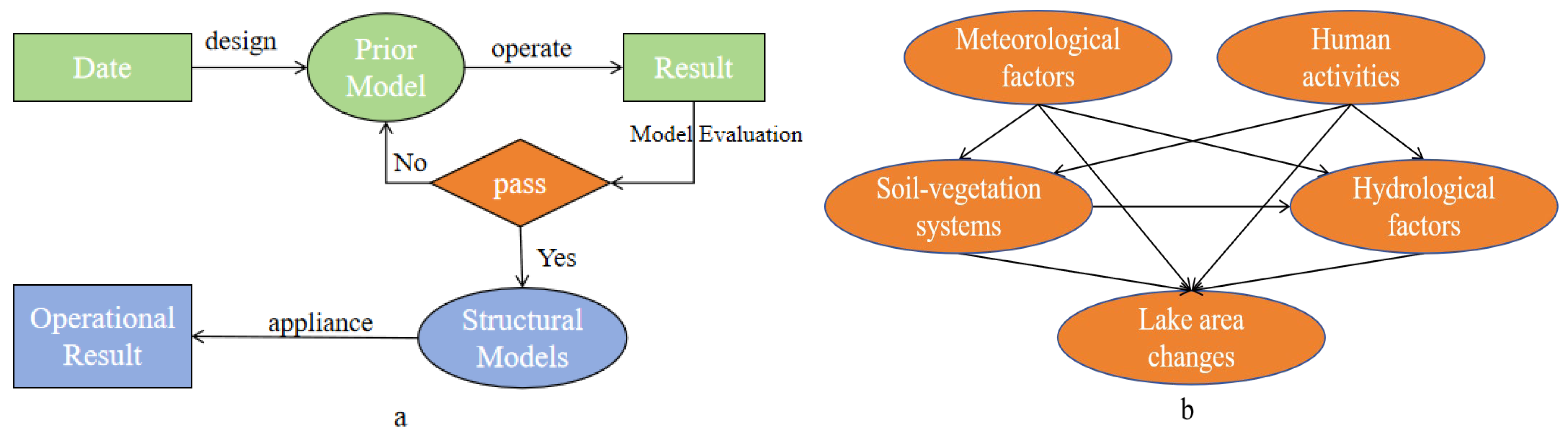
2.3.3. Methodology for the Study of Mechanisms Driving Changes in Lake Area

This study uses PLS-SEM to treat 60 samples of data (May–October monthly data from 2011 to 2020). The vital step before running Structural Equation Modeling is to find a suitable structural model for this study, and its structural design process is shown in Figure 3a. Initially, we constructed an empirical model utilizing the attributes of the gathered data, subsequently executing it and assessing its structural performance. Failure to adopt the evaluation requires adjustment of the model a priori until the model a priori adopts the model evaluation. Finally, Structural Equation Modeling through prior modeling will be applied to reveal complex causality studies.

For the study of the area-driven study of Ebinur Lake, “Meteorological factors”, “Soil–vegetation system”, “Hydrology factor”, and “Human activities” were selected as latent variables for the PLS-SEM study. All four latent variables are directly affected by changes in the area of Ebinur Lake, so they are directly linked to “Lake area changes”. In addition, “Meteorological factors” and “Human activities” also have an impact on “Soil–vegetation systems” and “Hydrological factors”, which are therefore linked in the design of the structural model. Thus, when designing the structural model, they are connected one by one. The “Soil–vegetation system” usually includes cropland, forest–grassland, and the Normalized Difference Salinity Index. The seasonal changes in these types of land will lead to the changes in their water demand characteristics, which will lead to the changes in “Hydrological factors”; thus, these two latent variables should be connected. It is difficult for the effect of “Human activities” to lead to changes in “Meteorological factors” in a short period of time, so these two latent variables are not connected. Ultimately, the final structure of the Ebinur Lake area change driver model is shown in Figure 3b.

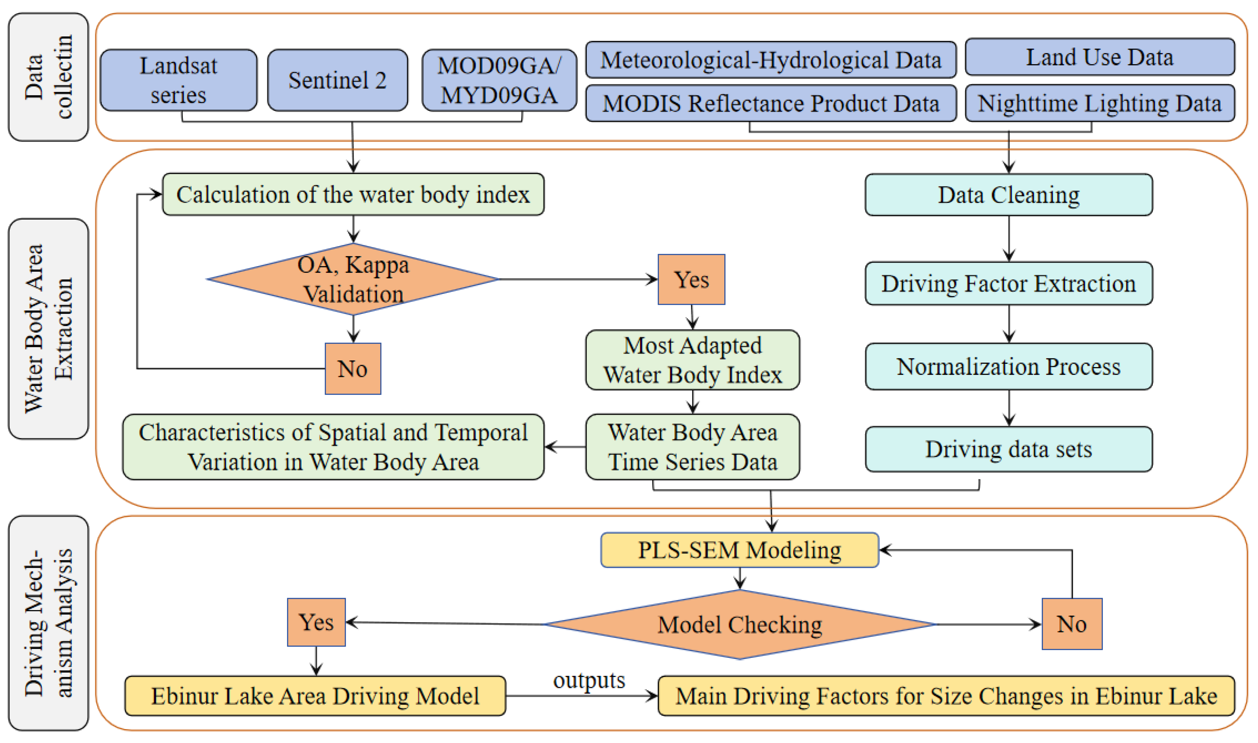
2.3.4. Analytical Work Flow

This study relies on the GEE cloud remote-sensing platform and uses Landsat, Sentinel 2, and MOD09GA/MYD09GA data to extract the area of the water body of Ebinur Lake by applying the NDWI, MNDWI, AWEI, and MAWEI. Thresholds and lake shorelines were optimized by the Maximum Interclass Variance method and Canny algorithm, and the best extraction method was selected by comparison. The inter-monthly spatial and temporal evolution of the water body of Ebinur Lake from 2009 to 2023 is revealed using the distance horizon method and center of gravity analysis. Further, the PLS-SEM approach was utilized to quantitatively ascertain the primary factors influencing the variation in Ebinur Lake’s water body area, incorporating hydrological, meteorological, and soil–vegetation systems, and human activities. The methodological framework of this study is depicted in Figure 4.

3. Results and Analysis

3.1. Analysis of Temporal and Spatial Changes

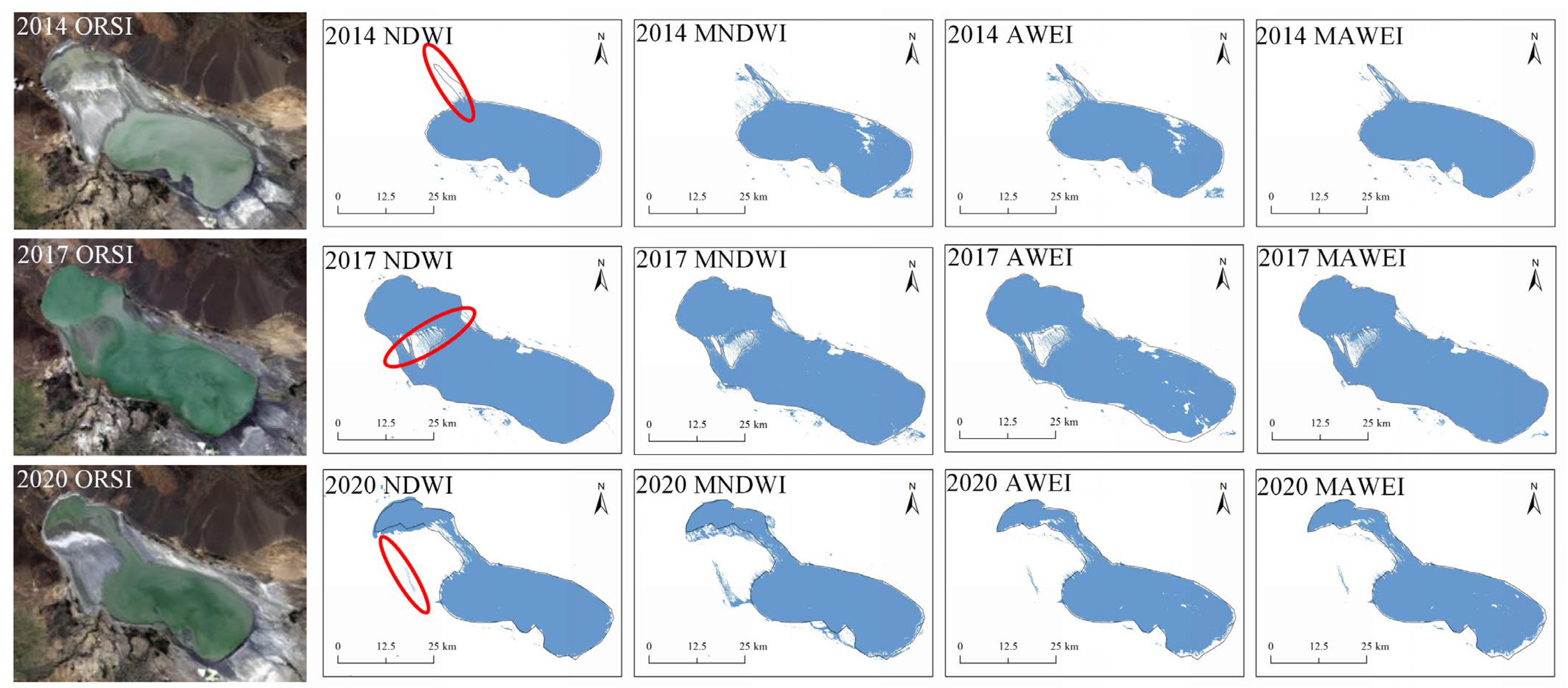
3.1.1. Determination of the Index of Adapted Water Bodies

In this research, three images, from June 2014, 2017, and 2020, were chosen to compare the outcomes of four water body index derivations, as presented in Figure 5. Three months of data were selected for validating lake area extraction accuracy. June’s imagery has a high quality and few clouds, which is beneficial for extraction. The lake areas in 2017, 2014, and 2020 vary greatly, from largest to smallest. This data combination represents multiple scenarios, ensuring reliable accuracy validation. All four water body indexes, NDWI, MNDWI, AWEI, and MAWEI, were found capable of effectively classifying water bodies and nonwater bodies, extracting the main convergence contours of Ebinur Lake by wave calculation, determining thresholds, and optimizing the lake shoreline, but there were some errors in extracting areas such as the fine water bodies, transition zones, and the bottom of the dry lake. Therefore, when establishing the confusion matrix, some typical points were selected in the areas of fine water bodies and transition zones to verify the water body extraction accuracy. It was discovered that the NDWI extraction results had partial mis-scoring for some fine water bodies; MNDWI extraction is less sensitive to dry lake bottoms and will incorrectly classify them as water bodies; AWEI extraction results will recognize some dry lakes and salty areas as water bodies and have higher threshold requirements; and MAWEI extraction of fine water bodies is more advantageous.

The confusion matrix is a standard program used to represent the overall accuracy and Kappa coefficient of each water body index for accuracy evaluation. The overall accuracy and Kappa coefficients of the three-phase images are shown in Figure 6a, and the growth rate of each water body index is calculated using the lower value of water body accuracy as a benchmark, as shown in Figure 6b. The overall accuracy of all four water body indexes is more than 90%, and the Kappa coefficients are MAWEI > NDWI > MNDWI > AWEI in descending order. In summary, the extraction effects of the water body indices follow a descending order as MAWEI > NDWI > MNDWI > AWEI. Thus, the MAWEI is adopted to delineate the area occupied by Ebinur Lake. During the COVID-19 pandemic, industrial disruptions and increased domestic water use, along with social–economic changes, disrupted the balance of the lake’s water supply in the catchment area. This led to a reduction in inflow and a decline in Ebinur Lake’s area from 2021 to 2023.

3.1.2. Characteristics of Temporal Changes in Water Body Area

After the above comparative analysis, the water bodies of Ebinur Lake were extracted month by month (May–October) for the last 15 years using MAWEI combined with the Maximum Between-Class Variance and Canny algorithm, respectively, and the results of the extraction are shown in Figure 7, which clearly shows that the water body of Ebinur Lake has drastic inter-monthly and inter-annual variations in area. While the water body in the large Ebinur Lake area is relatively stable, the northwest small lake area and transition area vary drastically.

Based on the above extraction results, the spatial statistics tool was used in ArcGIS 10.8 to calculate an area of the lake, and the resultant area of the lake was used to draw a line graph (as shown in Figure 8a). From the figure, it can be seen that the area of Ebinur Lake shows a slow increasing trend from 2009 to 2017 and a significant decreasing trend from 2017 to 2023, with the largest area in 2017. Trace something to its source: First, the 2015–2016 El Niño brought more winter snowfall, which increased glacial meltwater and thus expanded the lake area in 2017. Second, the revision of the Xinjiang Water Resource Protection Regulations, the restriction of cotton planting, and the promotion of drip irrigation saved water for the lake. These factors jointly contributed to the change in 2017. The three months of May, July, and September of each year were selected for this study to represent spring, summer, and autumn, and trends were plotted against the average lake area during the year (Figure 8b). As depicted in Figure 8b, there is a distinct variation in seasonal area sizes, with spring exhibiting the largest area, followed by summer, and then autumn. The trend of change in area shows a change in fluctuation with an increase and then a decrease.

According to the monthly area data from 2009 to 2023, the average value of the area of the water body was obtained as 493.59 km², and the distance level analysis yielded the annual distance level plot in Figure 8c and the monthly distance level value in Figure 8d. The annual expansion and contraction trend of the lake can be seen from the distance level values, which showed negative growth rates of −14.15% and −10.23% between 2009 and 2010. Between 2011 and 2012, the annual parity values showed positive growth rates of 4.93% and 10.51%. In the years 2013–2015 and 2020–2023, the annual distance parity values showed negative growth in each year, with the highest negative growth rate of −55.41% in 2023. In 2016–2019, the annual distance parity values showed positive growth rates of more than 15 percent, with 2017 reaching the maximum growth value of 51 percent in the last 15 years. By analyzing the value of the distance level in each month, the trend of the water body area change in each month can be obtained. Figure 8d shows that, in most cases, the largest distance level value is in May while the corresponding smallest value is in October, with the distance level value decreasing roughly with the increase in the month. The absolute variation in the water body area of Ebinur Lake fluctuates between −400 and 400 km², with the distance horizon value being more in the negative region during 2009–2012 and 2020–2023, but with values fluctuating in the positive region during 2016–2019.

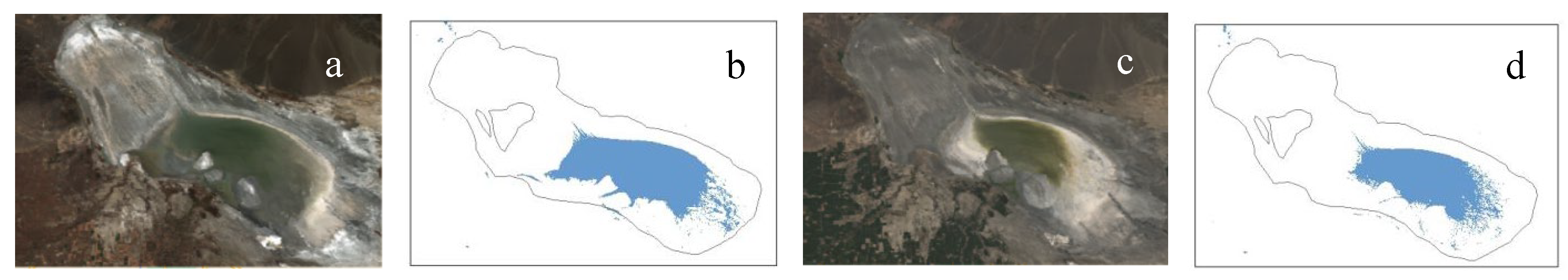
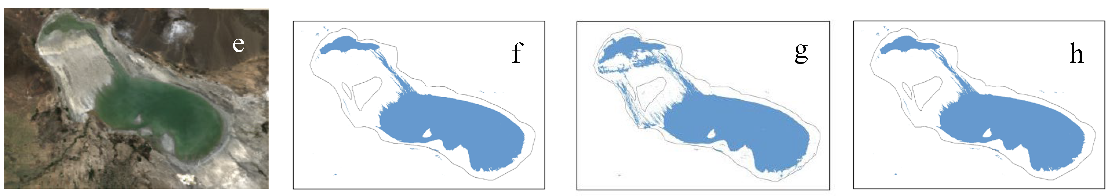
3.1.3. Characterization of Spatial Variability in Lake Water Bodies

This research examines the spatiotemporal variations in Ebinur Lake between 2009 and 2023, employing the center-of-gravity analysis approach, which consolidates alterations in the lake’s primary region into a cohesive picture (Figure 9a). From Figure 9b, it can be observed that, in general, the center of gravity of Ebinur Lake from 2009 to 2023 is transferred from the southeast to the northwest, which is back to the southeast from the northwest, and the northernmost point of the center of gravity (the center-of-gravity point of 2017) is at a greater distance from the southernmost point (the center-of-gravity point of 2015), with the lake’s area generally depicting expansion and then shrinkage of the lake. The smallest migration of the center of gravity was between 2009 and 2010 (0.27 km), followed by a movement of the Ebinur Lake center of gravity northward in a straight line (Figure 9c); it declined in 2013, with a small migration occurring in 2014, still towards the south (Figure 9d); the largest amount of change in the migration of the center of gravity was between 2015 and 2016 (8.1 km), when the center of gravity shifted from its original southeastern location to the northwestern part of the country, and reached its northernmost point in this 15-year period in 2017 (Figure 9e). The area of the center of gravity of Ebinur Lake gradually shifted southward from 2017, reaching another large value of 4.6 km for the center-of-gravity migration distance between 2019 and 2020, with the center of gravity continuing to move downward albeit with a decreasing rate between 2020 and 2023 (Figure 9f). In the majority of cases, the northwest corner of the small lake area and the transition area has a certain water body area in May–June, but in July–August, the area gradually dries out, resulting in a decrease in the overall area of the water body of Ebinur Lake, but in September-October, the area of the water body of Ebinur Lake tends to stabilize, with little variation.

3.2. Analysis of the Drivers of Change in Water Body Size in Ebinur Lake

Excluded were the measurement variables with significant collinearity to ensure their VIF ≤ 3.3 [35,54]. The prior model underwent iterative refinements until the required parameters for the driving PLS-SEM test were all met (

Table 3. Parameters of PLS-SEM test for changes in lake area of Ebinur Lake.

Latent Variable	R2	Q2
Soil–vegetation systems	0.589	0.441
Hydrological factors	0.674	0.248
Lake area changes	0.745	0.717

). Table 3 shows that the R² of the latent variable “Soil–vegetation systems” is 0.589, the R² of “Hydrological factors” is 0.674, and the R² of “Lake area changes” is 0.745, and all the endogenous latent variables have a Q² greater than zero. Since the Q² values for all endogenous latent variables surpassed zero, this indicates that the model exhibits favorable predictive performance.

Findings from the lake-size-driven PLS-SEM runs for Ebinur Lake are shown in Figure 10a. Green dashed arrows signify non-significant correlations between latent variables, whereas solid blue lines depict statistically significant relationships among these variables. The numerals on arrows linking latent variables depict the positional factor, whereas the numerals on arrows connecting measured variables to latent variables represent the external weights. Figure 8a demonstrates that, among the drivers of changes in Ebinur Lake’s water body area, the latent variable labeled “Meteorological factors” has a robust direct positive impact on both “Hydrological factors” and the “Soil–vegetation systems”. The latent variable “Human activities” showed a positive effect on “Hydrological factors” and a negative effect on “Soil–vegetation systems”, and the former effect was significant. For the water body area of Ebinur Lake, the latent variables “Soil–vegetation systems” and “Meteorological factors” showed a significant negative effect, and “Hydrological factors” showed a significant positive effect, while “Human activities” showed a significant positive effect on “Soil–vegetation systems”. However, the direct effect of “Human activities” was not significant.

In the PLS-SEM analysis of driving factors influencing changes in the Ebinur Lake region, the direct influence is indicated by the path coefficients linking the two latent variables. Conversely, the indirect influence is reflected in the product of path coefficients along each intermediary path. The disaggregation of direct and indirect effects yields a visual portrayal of the interconnectedness among the latent variables, facilitating a clear and precise understanding of their relationships. Figure 10b demonstrates that, apart from the direct impact of “Meteorological factors” on “Hydrological factors”, there is also an indirect influence transmitted through the “Soil–vegetation systems”, yielding an indirect effect magnitude of 0.277. The effect of “Human activities” on “Hydrological factors” is the same as the effect of “Meteorological factors” on “Hydrological factors” with an indirect effect of −0.006. The “Soil–vegetation systems” influences the variation in Ebinur Lake’s water body area through both direct and indirect pathways, exhibiting a negative direct effect (−0.116) and a contrasting positive indirect effect (0.417). Conversely, “Human activities” affect the water body area change in Ebinur Lake in four distinct ways, contributing a positive direct effect (0.151) alongside a minor direct effect of 0.052. Similarly, “Meteorological factors” exert influence through four pathways, with a negative direct effect (−0.379) and a substantial positive indirect effect (0.519).

When analyzing the impact of each underlying variable on changes in Ebinur Lake’s water body area, it is crucial to understand that the total effect between any two such variables is the sum of their direct and indirect influences. In terms of latent variables, “Hydrological factors” has the most significant control on the size of the water body of Ebinur Lake (with a total effect of 1.158), followed by “Soil–vegetation systems” (with a total effect of 0.301) and then by “Human activities” (with a total effect of 0.203) and “Meteorological factors” (with a total effect of 0.140) (Figure 10b). Figure 10b presents a hierarchical breakdown of the contributions of various potential variables to the variation in the water body area of Ebinur Lake. Specifically, “Hydrological factors” emerged as the most significant contributor, accounting for 64.3%, followed by the “Soil–vegetation systems” with 16.7%, “Human activities” with 11.3%, and “Meteorological factors” contributing the least at 7.8%, in descending order of importance.

The weights attributed to the measurement variables reflect the degree of their influence on the target variables. When considering the “Meteorological factors” measurement variables, wind speed at Alashankou emerges as the foremost influential factor (0.540), closely followed by air temperature (0.526). The subsequent variables, listed in descending order of significance, are precipitation (0.206), wind speed at the Jinghe River (0.141), aerosol (0.097), and evapotranspiration (0.072). Among the measurement variables of “Human activities”, construction land has the highest weighting coefficient in absolute value (0.891), followed by nighttime light (−0.507) and cultivated land (0.018), with nighttime light showing a negative effect on the area of the water body of Ebinur Lake. The largest weighting coefficient of the measurement variables of “Soil–vegetation systems” was the NDVI of forest–grassland (0.712), followed by the NDSI (0.545) and NDVI of cropland (−0.262), with the NDVI of cropland having a negative effect on the area of the water body. Regarding the “Hydrological factors” under investigation, the total inflow to the lake (0.812) exhibited a more substantial positive influence on the water body’s area than the lake surface water temperature (0.515), while the impact of the water level (−0.018) was the least pronounced in a negative direction. By integrating the overall effect’s relative contribution with the assigned weighting coefficients, it was determined that the total inflow to the lake had the greatest impact on the lake’s area.

4. Discussion

4.1. Water Body Extraction Threshold Determination and Resolution Inconsistency Issues

The determination of water extraction thresholds is critically influenced by spectral characteristics, atmospheric conditions, and sensor parameters. Ebinur Lake is a shallow (<2 m mean depth) brackish lake in northwest China [55], and it presents four compounding challenges for threshold-based water delineation: (1) transitional zones from >30% seasonal area variations create mixed pixels that hinder threshold selection [56]; (2) hypersalinity (87 g/L) modifies near-infrared reflectance characteristics, reducing water/land contrast essential for automated extraction [57]; (3) atmospheric turbidity from 165 annual dusty days at the Alashankou wind corridor degrades spectral fidelity through particulate scattering; and (4) temporal gaps in 16-day Landsat revisits mismatch the lake’s rapid area dynamics. These factors collectively introduce >15% uncertainty in area extraction (78–82% accuracy vs. field measurements), particularly during aeolian events and seasonal transitions.

The water body MAWEI constructed in this study applies the Maximum Between-Class Variance method to determine the threshold value, and the Canny algorithm is used to optimize the selection of the water body boundaries, which can circumvent a part of the problem of unsatisfactory water body extraction results due to the threshold value. When using the Canny algorithm, it is also necessary to utilize the Otsu method to determine the high and low thresholds, as the accuracy of these three thresholds will influence the results of water body extraction directly. During water extraction, suitability thresholds vary at different times due to image quality and environmental conditions that require constant adjustment. The results extracted in this study incorporate a classification of post-processing tools, which are somewhat subjective.

This study used the Otsu method and Canny algorithm method to optimize the lake shoreline, to gain a clearer water body boundary. However, for the dry season, the water body boundary is not so obvious (Figure 11a–d). Some of the areas with more severe salinization are also identified as water bodies, bringing uncertainty to the area statistics. Therefore, this study employs masking to cover severely salinized areas, thereby enhancing the accuracy of water body extraction.

In response to the problem of different spatial resolutions of remote-sensing data, it was mentioned above that all images were sampled up to 30 m, which to some extent ensured that remote-sensing data were comparable at the same scale. As the band resolution of Sentinel 2 varies, it has a certain impact on water body extraction. In this paper, the resolution of the Sentinel 2 shortwave infrared band is resampled to 10 m. Then, the water body is extracted using the method described in this paper. Finally, all the results are resampled to 30 m. However, in the process of selecting suitable water body indexes, it was found that when using Sentinel 2 remote-sensing data to extract water bodies, the accuracy of the water body NDWI extraction results was essentially the same as that of the above-mentioned first sample in the extraction accuracy (Figure 11e–h).

4.2. Analysis of the Controlling Factors for Changes in the Size of Ebinur Lake

Hydrological factors contributed most significantly to area variations in Ebinur Lake, accounting for 64.3% of observed changes, with the total inflow volume identified as the dominant positive driver. As a terminal lake, Ebinur Lake primarily receives water from the Bortala River and Jing River. Increased inflow has been conclusively shown to directly drive lake expansion [44]. The rapid influx of cold meltwater induces transient surface cooling, reducing evaporation rates, and causes areal enlargement [58]. Counteracting this trend, water-level fluctuations demonstrate seasonally modulated impacts: monsoonal and snowmelt-driven rises enhance surface area, whereas winter ice formation creates apparent spatial expansion despite a diminished water retention capacity due to hydrological discontinuity [59,60].

Soil–vegetation systems had a secondary impact on the variation in Ebinur Lake’s area, with a contribution rate of 16.7%, in which forest–grassland played a particularly prominent role. Forest–grassland reduces runoff velocity and enhances water infiltration by increasing surface roughness and porosity, thereby decreasing runoff evaporation and loss [61]. Meanwhile, it lowers surface reflectivity and evapotranspiration to regulate local microclimates [62]. Under the guidance of ecological conservation policies, the protection of forest–grassland has been strengthened. Additionally, the increase in the Normalized Difference Salinity Index (NDSI) indicates intensified soil salinization, which suppresses vegetation growth and reduces soil water retention capacity, leading more water to enter the lake via surface runoff. While this may temporarily increase the lake area, it risks disrupting the ecological balance in the long term. The expansion of cropland land negatively correlates with the lake area due to water consumption reducing inflow.

Human activities contributed 11.3% to the variation in Ebinur Lake’s area, primarily exhibiting positive impacts. The expansion of construction land showed the most significant effect, as increased impermeable surfaces enhanced river runoff, thereby promoting lake water replenishment. Although cultivated land expansion might indirectly increase lake water through irrigation return flow or groundwater lateral recharge, its net effect requires comprehensive evaluation considering the regional water balance [47]. Increased nighttime light intensity, which is an indicator of population density, leads to a surge in water demand, which in turn has an impact on river runoff [63]. In conclusion, different factors related to human activities have diverse impacts on the area of Ebinur Lake. They are not contradictory but rather reflect the complexity of human activities’ influence on the lake ecosystem.

In contrast, “Meteorological factors” demonstrated the smallest contribution to lake area variations. Their complexity lies in conflicting direct and indirect effects, highlighting the analytical advantages of PLS-SEM. Directly, meteorological factors exerted significant negative impacts on the lake area, particularly through wind speed at the Alashankou, temperature, and precipitation. Wind speed accelerates water surface evaporation, while rising temperatures intensify evaporation from both the lake and rivers, collectively lowering water levels. Although precipitation serves as a critical water source, accelerated evaporation under high temperatures coupled with insufficient rainfall will depress water levels. Simultaneously, altered precipitation patterns combined with human activities have reduced precipitation, further diminishing the lake area. The region’s characteristic high-evaporation–low-precipitation regime makes the combined effects of precipitation and evaporation the decisive factors in lake area dynamics.

4.3. Uncertainty Analysis and Outlook

This study employed the water body MAWEI combined with Maximum Interclass Variance and the Canny algorithm to achieve high-accuracy water body extraction for Ebinur Lake, addressing misclassification in high-brightness saline areas through regional masking. PLS-SEM analysis identified total inflow as the primary driver of lake area changes between 2011 and 2020. However, limitations include potential errors from spatiotemporal resolution aggregation and context-dependent applicability of the MAWEI [64]. Future research should focus on three key directions: improving driving data precision via ground validation and high-resolution imagery integration, incorporating socioeconomic variables to better quantify anthropogenic impacts, and systematically investigating declining riverine inputs—a critical hydrological trend observed in recent records that requires mechanistic exploration to enhance predictive modeling. These advancements will deepen understanding of Ebinur Lake’s dynamic responses to environmental and human-induced changes, informing sustainable basin management strategies.

5. Conclusions

In the investigation, data from Landsat imagery, Sentinel 2, and MOD09GA/MYD09GA were employed to assess the water body of Ebinur Lake. Indices including NDWI, MNDWI, AWEI, and MAWEI were chosen to measure the lake’s water surface area, depict its spatial and temporal shifts spanning the last 15 years, and delve into the main factors influencing these changes through the application of the PLS-SEM. The primary outcomes of the analysis are outlined as follows:

(1)

The water body extraction method used in this study, which combines MAWEI with the Otsu method and the Canny algorithm, can effectively identify the water area of Ebinur Lake.

(2)

The water area of Ebinur Lake has undergone drastic changes and generally shows a downward trend. In 2017, the area of Ebinur Lake reached its maximum value. The centroid of the lake area fluctuates back and forth from the southeast corner to the northwest corner. The area changes mainly occur in the small lake area and the transition zone.

(3)

Hydrological factors are the dominant factors in the area changes of Ebinur Lake, with a relative contribution rate of 64.3%. Among them, lake inflow has the greatest impact (0.812).

This study develops a methodological synergy combining the MAWEI, GEE cloud platform, and PLS-SEM to quantify Ebinur Lake’s spatiotemporal dynamics and dominant drivers. The framework enables high-precision water monitoring in saline–alkali environments and reveals inflow volume as the critical control on lake shrinkage.

References

1. Mechal, A.; Fekadu, D.; Abadi, B. Multivariate and water quality index approaches for spatial water quality assessment in Lake Ziway, Ethiopian Rift. Water Air Soil Pollut. 2024, 235, 78. [Google Scholar] [CrossRef]
2. Zhang, Z.; Chen, X.; Xu, C.Y.; Hong, Y.; Hardy, J.; Sun, Z. Examining the influence of river–lake interaction on the drought and water resources in the Poyang Lake basin. J. Hydrol. 2015, 522, 510–521. [Google Scholar] [CrossRef]
3. Ho, J.C.; Michalak, A.M.; Pahlevan, N. Widespread global increase in intense lake phytoplankton blooms since the 1980s. Nature 2019, 574, 667–670. [Google Scholar] [CrossRef]
4. Huang, L.; Liu, J.; Shao, Q.; Liu, R. Changing inland lakes responding to climate warming in Northeastern Tibetan Plateau. Clim. Change 2011, 109, 479–502. [Google Scholar] [CrossRef]
5. Qi, Z.; Cui, C.; Jiang, Y.; Chen, Y.; Ju, J.; Guo, N. Changes in the spatial and temporal characteristics of China’s arid region in the background of ENSO. Sci. Rep. 2022, 12, 17826. [Google Scholar] [CrossRef]
6. Li, Q.; Lu, L.; Wang, C.; Li, Y.; Sui, Y.; Guo, H. MODIS-derived spatiotemporal changes of major lake surface areas in arid Xinjiang, China, 2000–2014. Water 2015, 7, 5731–5751. [Google Scholar] [CrossRef]
7. Yao, F.; Livneh, B.; Rajagopalan, B.; Wang, J.; Crétaux, J.-F.; Wada, Y.; Berge-Nguyen, M. Satellites reveal widespread decline in global lake water storage. Science 2023, 380, 743–749. [Google Scholar] [CrossRef]
8. Hao, S.; Li, F.; Li, Y.; Gu, C.; Zhang, Q.; Qiao, Y.; Jiao, L.; Zhu, N. Stable isotope evidence for identifying the recharge mechanisms of precipitation, surface water, and groundwater in the Ebinur Lake basin. Sci. Total Environ. 2019, 657, 1041–1050. [Google Scholar] [CrossRef]
9. Wei, Q.; Halike, A.; Yao, K.; Chen, L.; Balati, M. Construction and optimization of ecological security pattern in Ebinur Lake Basin based on MSPA-MCR models. Ecol. Indic. 2022, 138, 108857. [Google Scholar] [CrossRef]
10. Zhang, F.; Tiyip, T.; Johnson, V.C.; Kung, H.; Ding, J.; Zhou, M.; Fan, Y.; Kelimu, A.; Nurmuhammat, I. Evaluation of land desertification from 1990 to 2010 and its causes in Ebinur Lake region, Xinjiang China. Environ. Earth Sci. 2015, 73, 5731–5745. [Google Scholar] [CrossRef]
11. Wang, H.; Qi, Y.; Lian, X.; Zhang, J.; Yang, R.; Zhang, M. Effects of climate change and land use/cover change on the volume of the Qinghai Lake in China. J. Arid. Land 2022, 14, 245–261. [Google Scholar] [CrossRef]
12. Zhang, S.; Pavelsky, T.M. Remote sensing of lake ice phenology across a range of lakes sizes, ME, USA. Remote Sens. 2019, 11, 1718. [Google Scholar] [CrossRef]
13. Zhang, F.; Tiyip, T.; Johnson, V.C.; Kung, H.-T.; Ding, J.-L.; Sun, Q.; Zhou, M.; Kelimu, A.; Nurmuhammat, I.; Chan, N.W. The influence of natural and human factors in the shrinking of the Ebinur Lake, Xinjiang, China, during the 1972–2013 period. Environ. Monit. Assess. 2015, 187, 4128. [Google Scholar] [CrossRef] [PubMed]
14. Bao, A.; Mu, G.; Zhang, Y.; Feng, X.; Chang, C.; Yin, X. Estimation of the rational water area for controlling wind erosion in the dried-up basin of the Ebinur Lake and its effect detection. Chin. Sci. Bull. 2006, 51, 68–74. [Google Scholar] [CrossRef]
15. Lemenkova, P. Monitoring seasonal fluctuations in saline lakes of Tunisia using Earth observation data processed by GRASS GIS. Land 2023, 12, 1995. [Google Scholar] [CrossRef]
16. Li, K.; Wang, J.; Yao, J. Effectiveness of machine learning methods for water segmentation with ROI as the label: A case study of the Tuul River in Mongolia. Int. J. Appl. Earth Obs. Geoinf. 2021, 103, 102497. [Google Scholar] [CrossRef]
17. Acharya, T.D.; Subedi, A.; Lee, D.H. Evaluation of water indices for surface water extraction in a Landsat 8 scene of Nepal. Sensors 2018, 18, 2580. [Google Scholar] [CrossRef]
18. Wang, Z.; Liu, J.; Li, J.; Zhang, D.D. Multi-spectral water index (MuWI): A native 10-m multi-spectral water index for accurate water mapping on Sentinel-2. Remote Sens. 2018, 10, 1643. [Google Scholar] [CrossRef]
19. Goffi, A.; Stroppiana, D.; Brivio, P.A.; Bordogna, G.; Boschetti, M. Towards an automated approach to map flooded areas from Sentinel-2 MSI data and soft integration of water spectral features. Int. J. Appl. Earth Obs. Geoinf. 2020, 84, 101951. [Google Scholar] [CrossRef]
20. Ouma, Y.O.; Tateishi, R. A water index for rapid mapping of shoreline changes of five East African Rift Valley lakes: An empirical analysis using Landsat TM and ETM+ data. Int. J. Remote Sens. 2006, 27, 3153–3181. [Google Scholar] [CrossRef]
21. McFeeters, S.K. The use of the Normalized Difference Water Index (NDWI) in the delineation of open water features. Int. J. Remote Sens. 1996, 17, 1425–1432. [Google Scholar] [CrossRef]
22. Xu, H. A study on information extraction of water body with the modified normalized difference water index (MNDWI). J. Remote Sens. Beijing 2005, 9, 595. (In Chinese) [Google Scholar] [CrossRef]
23. Feyisa, G.L.; Meilby, H.; Fensholt, R.; Proud, S.R. Automated Water Extraction Index: A new technique for surface water mapping using Landsat imagery. Remote Sens. Environ. 2014, 140, 23–35. [Google Scholar] [CrossRef]
24. Wang, H.; Wang, J.; Cui, Y.; Yan, S. Consistency of Suspended Particulate Matter Concentration in Turbid Water Retrieved from Sentinel-2 MSI and Landsat-8 OLI Sensors. Sensors 2021, 21, 1662. [Google Scholar] [CrossRef]
25. Zhou, Y.; Zhang, L.; Wang, Y. Monitoring of water extent and variation of the Poyang lake using GF-1 remote sensing data. In Proceedings of the 2017 7th International Conference on Manufacturing Science and Engineering (ICMSE 2017), Zhuhai, China, 11–12 March 2017; pp. 384–387. [Google Scholar] [CrossRef]
26. Moknatian, M.; Piasecki, M.; Gonzalez, J. Development of geospatial and temporal characteristics for Hispaniola’s Lake Azuei and Enriquillo using Landsat imagery. Remote Sens. 2017, 9, 510. [Google Scholar] [CrossRef]
27. Chen, K.; Liu, X.; Chen, X.; Guo, Y.; Dong, Y. Spatial characteristics and driving forces of the morphological evolution of East Lake, Wuhan. J. Geogr. Sci. 2020, 30, 583–600. [Google Scholar] [CrossRef]
28. Khazaei, B.; Khatami, S.; Alemohammad, S.H.; Rashidi, L.; Wu, C.; Madani, K.; Kalantari, Z.; Destouni, G.; Aghakouchak, A. Climatic or regionally induced by humans? Tracing hydro-climatic and land-use changes to better understand the Lake Urmia tragedy. J. Hydrol. 2019, 569, 203–217. [Google Scholar] [CrossRef]
29. Tao, S.; Fang, J.; Ma, S.; Cai, Q.; Xiong, X.; Tian, D.; Zhao, X.; Fang, L.; Zhang, H.; Zhu, J.; et al. Changes in China’s lakes: Climate and human impacts. Natl. Sci. Rev. 2020, 7, 132–140. [Google Scholar] [CrossRef]
30. Zheng, L.; Xia, Z.; Xu, J.; Chen, Y.; Yang, H.; Li, D. Exploring annual lake dynamics in Xinjiang (China): Spatiotemporal features and driving climate factors from 2000 to 2019. Clim. Change 2021, 166, 36. [Google Scholar] [CrossRef]
31. Liu, H.; Chen, Y.; Ye, Z.; Li, Y.; Zhang, Q. Recent lake area changes in Central Asia. Sci. Rep. 2019, 9, 16277. [Google Scholar] [CrossRef]
32. Ding, X.; Zhang, H.; Wang, Z.; Shang, G.; Huang, Y.; Li, H. Analysis of the Evolution Pattern and Driving Mechanism of Lakes in the Northern Ningxia Yellow Diversion Irrigation Area. Water 2022, 14, 3658. [Google Scholar] [CrossRef]
33. Mo, H. Comprehensive evaluation of flood and flood in the Yellow River Basin based on gray correlation analysis. J. Geosci. Environ. Prot. 2021, 9, 13. [Google Scholar] [CrossRef]
34. Wieland, M.; Martinis, S.; Kiefl, R.; Gstaiger, V. Semantic segmentation of water bodies in very high-resolution satellite and aerial images. Remote Sens. Environ. 2023, 287, 113452. [Google Scholar] [CrossRef]
35. Jöreskog, K.G. A general method for estimating a linear structural equation system. ETS Res. Bull. Ser. 1970, 1970, I-41. [Google Scholar] [CrossRef]
36. Kim, W.; Moon, J.E.; Park, Y.J.; Ishizaka, J. Evaluation of chlorophyll retrievals from Geostationary Ocean color imager (GOCI) for the north-east Asian region. Remote Sens. Environ. 2016, 184, 482–495. [Google Scholar] [CrossRef]
37. Gao, S.; Lü, Y.; Jiang, X. Increased precipitation and vegetation cover synergistically enhanced the availability and effectiveness of water resources in a dryland region. J. Hydrol. 2025, 654, 132812. [Google Scholar] [CrossRef]
38. Liu, C.; Chen, Y.; Huang, W.; Fang, G.; Li, Z.; Zhu, C.; Liu, Y. Climate warming positively affects hydrological connectivity of typical inland river in arid Central Asia. npj Clim. Atmos. Sci. 2024, 7, 250. [Google Scholar] [CrossRef]
39. Du, B.; Wang, Z.; Mao, D.; Li, H.; Xiang, H. Tracking lake and reservoir changes in the Nenjiang watershed, Northeast China: Patterns, trends, and drivers. Water 2020, 12, 1108. [Google Scholar] [CrossRef]
40. Ma, M.; Wang, X.; Veroustraete, F.; Dong, L. Change in area of Ebinur Lake during the 1998–2005 period. Int. J. Remote Sens. 2007, 28, 5523–5533. [Google Scholar] [CrossRef]
41. Wang, Y.; Gu, X.; Yang, G.; Liao, N. Impacts of climate change and human activities on water resources in the Ebinur Lake Basin, Northwest China. J. Arid. Land 2021, 13, 581–598. [Google Scholar] [CrossRef]
42. Liu, C.; Zhang, F.; Tan, M.L.; Jim, C.-Y.; Song, K.; Shi, J.; Lin, X.; Kung, H.-T. High spatiotemporal resolution reconstruction of suspended particulate matter concentration in arid brackish lake, China. J. Clean. Prod. 2023, 414, 137673. [Google Scholar] [CrossRef]
43. Wang, J.; Ding, J.; Li, G.; Liang, J.; Yu, D.; Aishan, T.; Zhang, F.; Yang, J.; Abulimiti, A.; Liu, J. Dynamic detection of water surface area of Ebinur Lake using multi-source satellite data (Landsat and Sentinel-1A) and its responses to changing environment. Catena 2019, 177, 189–201. [Google Scholar] [CrossRef]
44. Liu, C.; Zhang, F.; Jim, C.Y.; Johnson, V.C.; Tan, M.L.; Shi, J.; Lin, X. Controlled and driving mechanism of the SPM variation of shallow Brackish Lakes in arid regions. Sci. Total Environ. 2023, 878, 163127. [Google Scholar] [CrossRef] [PubMed]
45. Akbas, A. Human or climate? Differentiating the anthropogenic and climatic drivers of lake storage changes on spatial perspective via remote sensing data. Sci. Total Environ. 2024, 912, 168982. [Google Scholar] [CrossRef]
46. Chen, J.; Chen, S.; Fu, R.; Li, D.; Jiang, H.; Wang, C.; Peng, Y.; Jia, K.; Hicks, B.J. Remote sensing big data for water environment monitoring: Current status, challenges, and future prospects. Earth’s Future 2022, 10, e2021EF002289. [Google Scholar] [CrossRef]
47. Foroumandi, E.; Nourani, V.; Kantoush, S.A. Investigating the main reasons for the tragedy of large saline lakes: Drought, climate change, or anthropogenic activities? A call to action. J. Arid. Environ. 2022, 196, 104652. [Google Scholar] [CrossRef]
48. Elvidge, C.D.; Zhizhin, M.; Ghosh, T.; Hsu, F.-C.; Taneja, J. Annual time series of global VIIRS nighttime lights derived from monthly averages: 2012 to 2019. Remote Sens. 2021, 13, 922. [Google Scholar] [CrossRef]
49. Elvidge, C.D.; Baugh, K.E.; Kihn, E.A.; Kroehl, H.W.; Davis, E.R. Mapping city lights with nighttime data from the DMSP Operational Linescan System. Photogramm. Eng. Remote Sens. 1997, 63, 727–734. [Google Scholar] [CrossRef]
50. Kalaiselvi, T.; Nagaraja, P.; Indhu, V. A comparative study on thresholding techniques for gray image binarization. Int. J. Adv. Res. Comput. Sci. 2017, 8, 1168–1172. [Google Scholar] [CrossRef]
51. Otsu, N. A threshold selection method from gray-level histograms. Automatica 1975, 11, 23–27. [Google Scholar] [CrossRef]
52. Canny, J. A computational approach to edge detection. IEEE Trans. Pattern Anal. Mach. Intell. 1986, 6, 679–698. [Google Scholar] [CrossRef]
53. Yang, N.; Li, J.; Mo, W.; Luo, W.; Wu, D.; Gao, W.; Sun, C. Water depth retrieval models of East Dongting Lake, China, using GF-1 multi-spectral remote sensing images. Glob. Ecol. Conserv. 2020, 22, e01004. [Google Scholar] [CrossRef]
54. de Anda, J.; Díaz-Torres, J.D.J.; Gradilla-Hernández, M.S.; de la Torre-Castro, L.M. Morphometric and water quality features of Lake Cajititlán, Mexico. Environ. Monit. Assess. 2019, 191, 92. [Google Scholar] [CrossRef]
55. Liu, Q.; Huang, C.; Shi, Z.; Zhang, S. Probabilistic river water mapping from Landsat-8 using the support vector machine method. Remote Sens. 2020, 12, 1374. [Google Scholar] [CrossRef]
56. Morshed, S.R.; Fattah, M.A. Responses of spatiotemporal vegetative land cover to meteorological changes in Bangladesh. Remote Sens. Appl. Soc. Environ. 2021, 24, 100658. [Google Scholar] [CrossRef]
57. Jiang, N.; Li, P.; Feng, Z. Remote sensing of swidden agriculture in the tropics: A review. Int. J. Appl. Earth Obs. Geoinf. 2022, 112, 102876. [Google Scholar] [CrossRef]
58. Yu, Z.; Yang, K.; Luo, Y.; Shang, C.; Zhu, Y. Lake surface water temperature prediction and changing characteristics analysis-A case study of 11 natural lakes in Yunnan-Guizhou Plateau. J. Clean. Prod. 2020, 276, 122689. [Google Scholar] [CrossRef]
59. Busker, T.; de Roo, A.; Gelati, E.; Schwatke, C.; Adamovic, M.; Bisselink, B.; Pekel, J.-F.; Cottam, A. A global lake and reservoir volume analysis using a surface water dataset and satellite altimetry. Hydrol. Earth Syst. Sci. 2019, 23, 669–690. [Google Scholar] [CrossRef]
60. Wang, J.; Yang, S.; Lou, H.; Liu, H.; Wang, P.; Li, C.; Zhang, F. Impact of lake water level decline on river evolution in Ebinur Lake Basin (an ungauged terminal lake basin). Int. J. Appl. Earth Obs. Geoinf. 2021, 104, 102546. [Google Scholar] [CrossRef]
61. Quan, Q.; Liang, W.; Yan, D.; Lei, J. Influences of joint action of natural and social factors on atmospheric process of hydrological cycle in Inner Mongolia, China. Urban Clim. 2022, 41, 101043. [Google Scholar] [CrossRef]
62. Huang, T.; Yu, D.; Cao, Q.; Qiao, J. Impacts of meteorological factors and land use pattern on hydrological elements in a semi-arid basin. Sci. Total Environ. 2019, 690, 932–943. [Google Scholar] [CrossRef] [PubMed]
63. Li, J.; Yu, Y.; Wang, X.; Zhou, Z. System dynamic relationship between service water and food: Case study at Jinghe River Basin. J. Clean. Prod. 2022, 330, 129794. [Google Scholar] [CrossRef]
64. Sun, W.C.; Wang, X.C.; Xu, Z.X. Research Progress and Prospect of Remote Sensing Estimation of River Discharge. Acta Geogr. Sin. 2024, 79, 565–583. (In Chinese) [Google Scholar] [CrossRef]
Figure 1. Schematic map of the study area ((a): location of Xinjiang, China; (b): comparison of water inflow into Ebinur Lake area; (c): schematic map of the Ebinur Lake watershed and the influence range of the change in the lake area; VWEL: water inflow into the lake; PTWEL: percentage of total water inflow into the lake; BR: inflow into the lake from the Boltara River; JR: inflow into the lake from the Jing River; ZP: inflow into the lake from the main canal; WZQ: inflow into the lake from the five branch canals; Total: total amount of water entering Ebinur Lake; P-farmland: percentage of farmland; P-building: percentage of buildings; P-water: percentage of water area; P-population: percentage of population; JAB: Alashankou City, Bole City, Shuanghe City, and Jinghe County; WC: Wenquan County).
Remotesensing 17 01431 g001
Figure 2. Map of data sources ((a): remote-sensing image data time-series distribution map; (b): number of images used in each sensor distribution).
Remotesensing 17 01431 g002
Figure 3. Ebinur Lake area change driving model ((a): Structural Equation Modeling design process; (b): final structure of Ebinur Lake area change driver model).
Remotesensing 17 01431 g003
Figure 4. The work flow of this study.
Remotesensing 17 01431 g004
Figure 5. Comparison of water body extraction accuracy using MAWEI, NDWI, and MNDWI indices. (Red areas indicate misclassified regions, including shoreline transition zones, desiccated lakebeds, and narrow tributaries).
Remotesensing 17 01431 g005
Figure 6. Validation of precision ((a): comparison of overall precision and Kappa coefficients for each index, (b): relative growth rate of water body precision in 2014; OA: overall accuracy).
Remotesensing 17 01431 g006
Figure 7. Monthly lake area extractions for Ebinur Lake from 2009 to 2023 (date labels are in 2009.05 format and represent May 2009; gray contours indicate historical maximum lake area for the 2009–2023 period).
Remotesensing 17 01431 g007
Figure 8. Time-series diagram of changes in the area of water bodies ((a): line graph of monthly area changes in Ebinur Lake, 2009–2023; (b): May, July, and September and average area changes over the last 15 years; (c): annual distance medians; (d) monthly distance medians; ZZL: percentage increase/decrease).
Remotesensing 17 01431 g008
Figure 9. Trajectories of center of gravity migration in Ebinur Lake from 2009 to 2023 ((a): general trend in the change in the center of gravity of Ebinur Lake from 2009 to 2023, (b): local zoom, (c): trend in the center of gravity of Ebinur Lake from 2009 to 2012, (d): graph of the trend in the change in the center of gravity from 2012 to 2015, (e): trend change from 2015 to 2017, (f): trend change from 2017 to 2023).
Remotesensing 17 01431 g009
Figure 10. SEM-PLS model results and contribution rates ((a): SEM-PLS model results plots in which *, **, and *** denote passing 0.1, 0.05, and 0.001 significance tests, respectively; (b): relative contributions of direct, indirect, and total effects among potential variables).
Remotesensing 17 01431 g010
Figure 11. Comparison of extracted boundaries of Ebinur Lake ((ad): October 2021 and October 2023 imagery and their extraction results; (e): June 2021 Sentinel 2 imagery; (f): NDWI extraction results; (g): MAWEI unsampled pre-extraction results; (h); MAWEI post-sampling results).
Remotesensing 17 01431 g011aRemotesensing 17 01431 g011b