
Multi-Object Feature Extraction in Resonance Region Based on Short-Time Matrix Pencil Method


Abstract
1. Introduction
2. Scenario and Method Description
2.1. Scattering Echo Characteristic
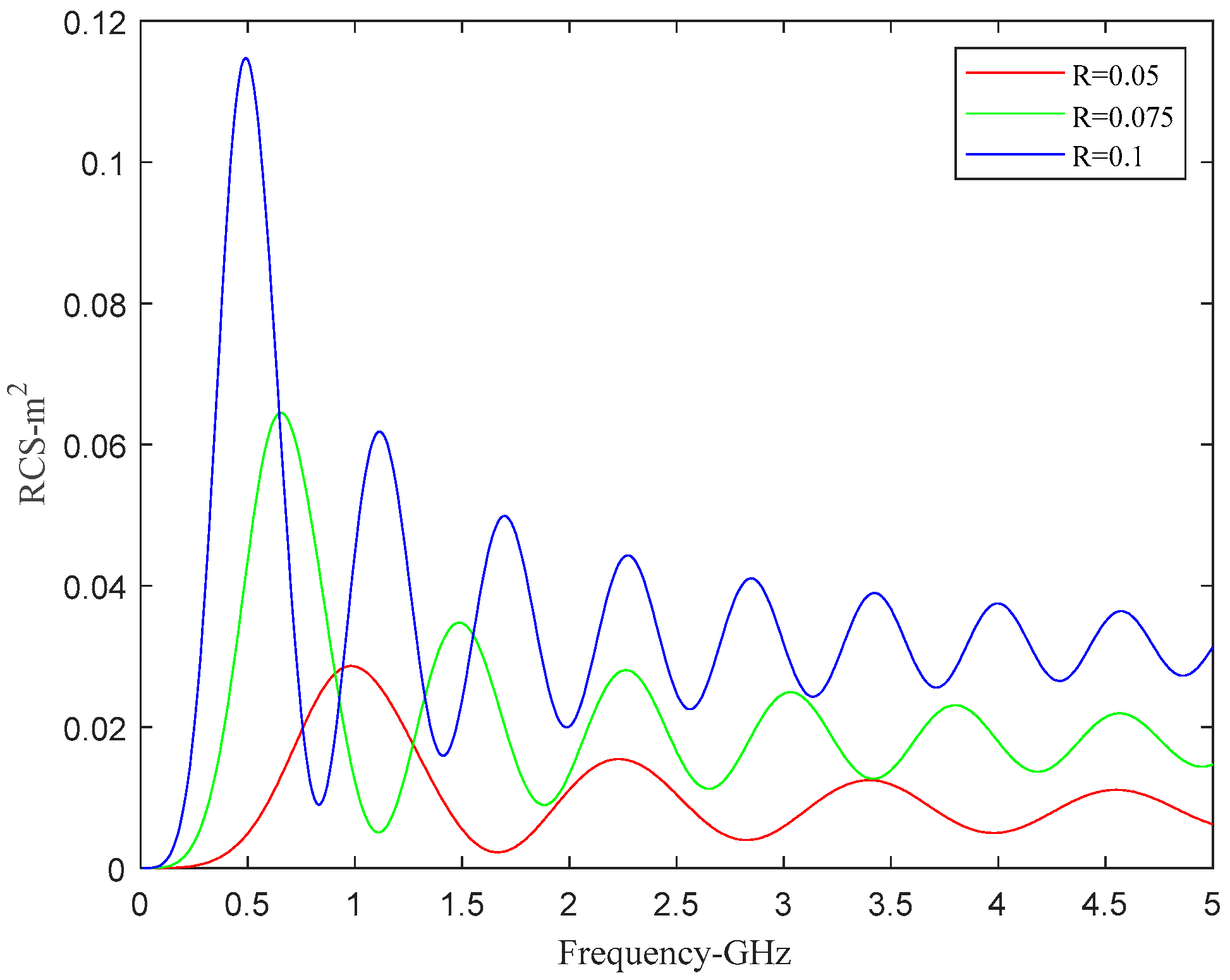
2.1.1. Single Target
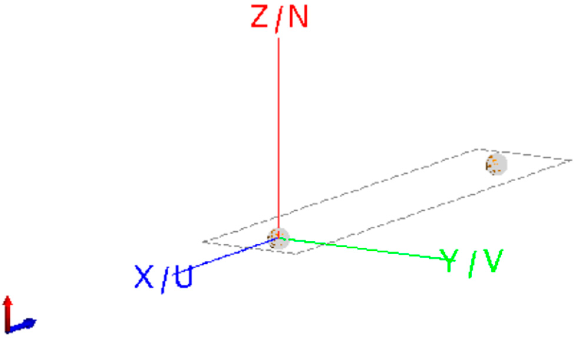
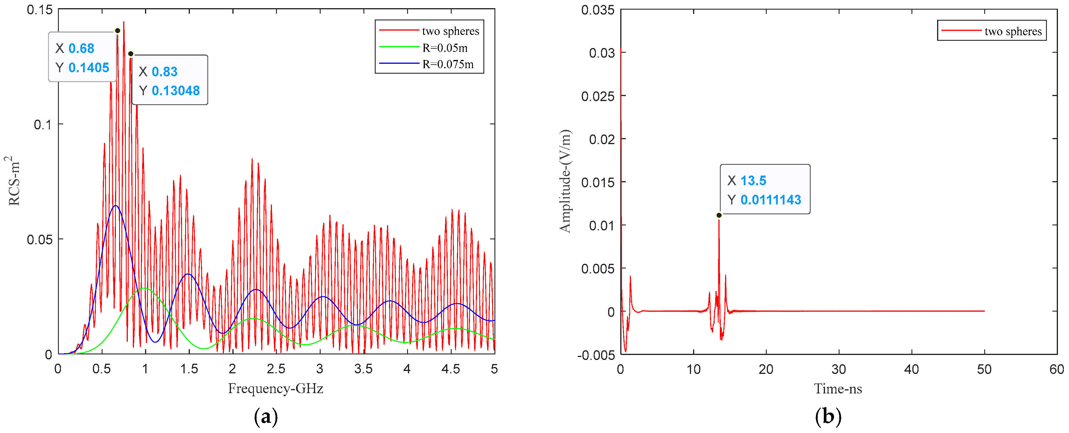
2.1.2. Multiple Targets
2.2. The Method to Extract the Pole Information
2.2.1. Matrix Pencil Method for Single Target
2.2.2. Short-Time Matrix Pencil Method for Multiple Targets
3. Results
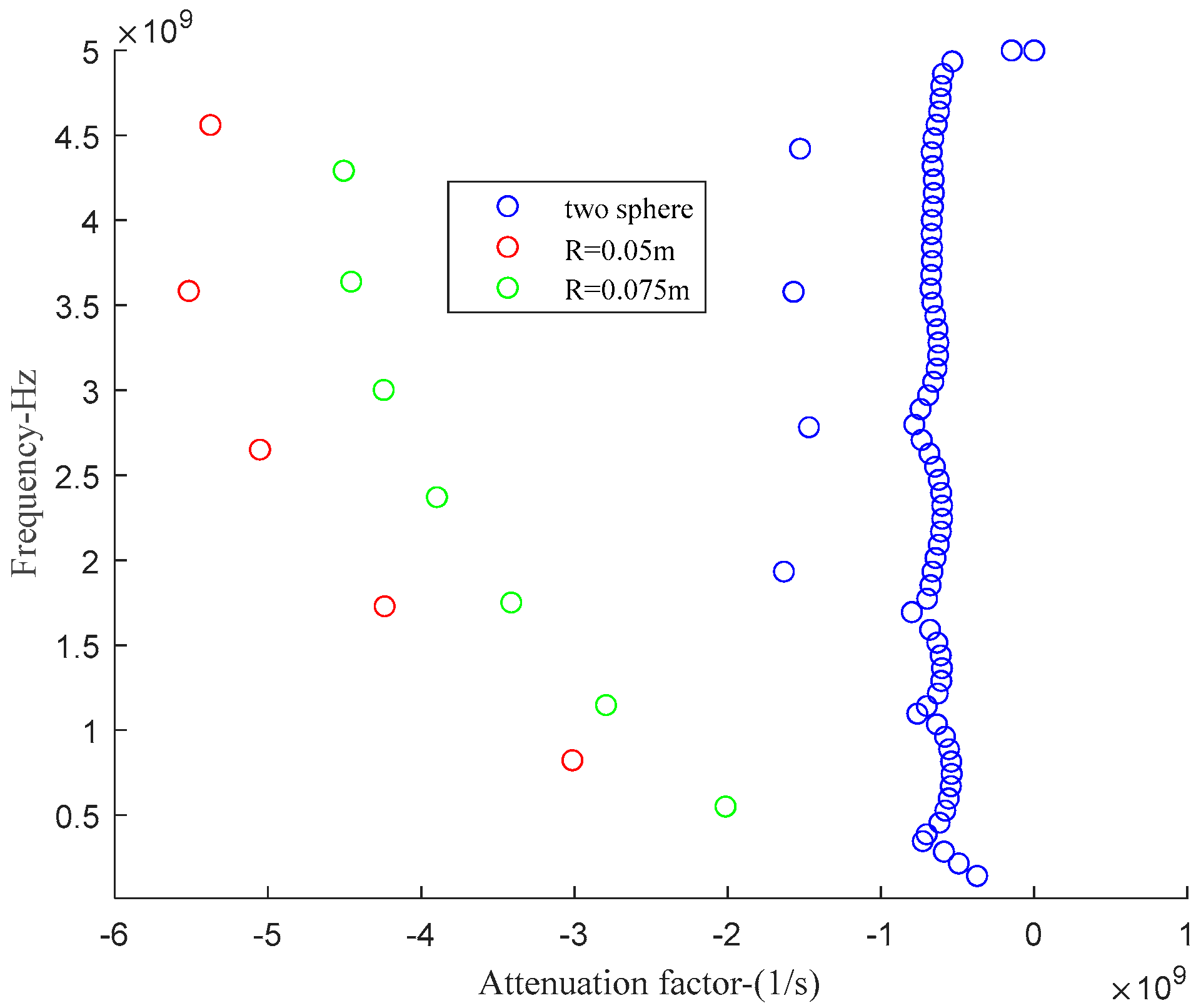
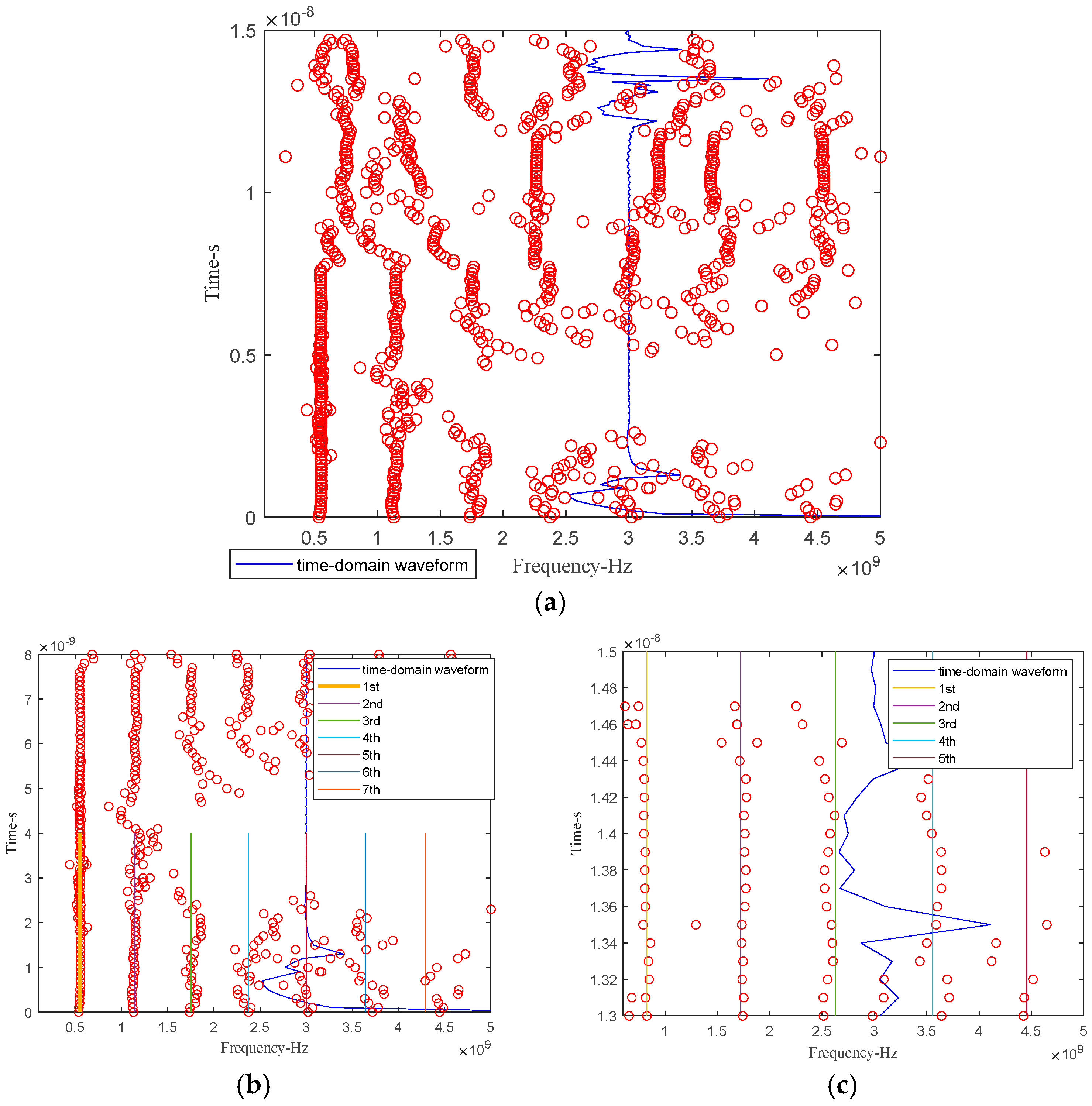
3.1. Electromagnetic Scattering Echo Data Analysis
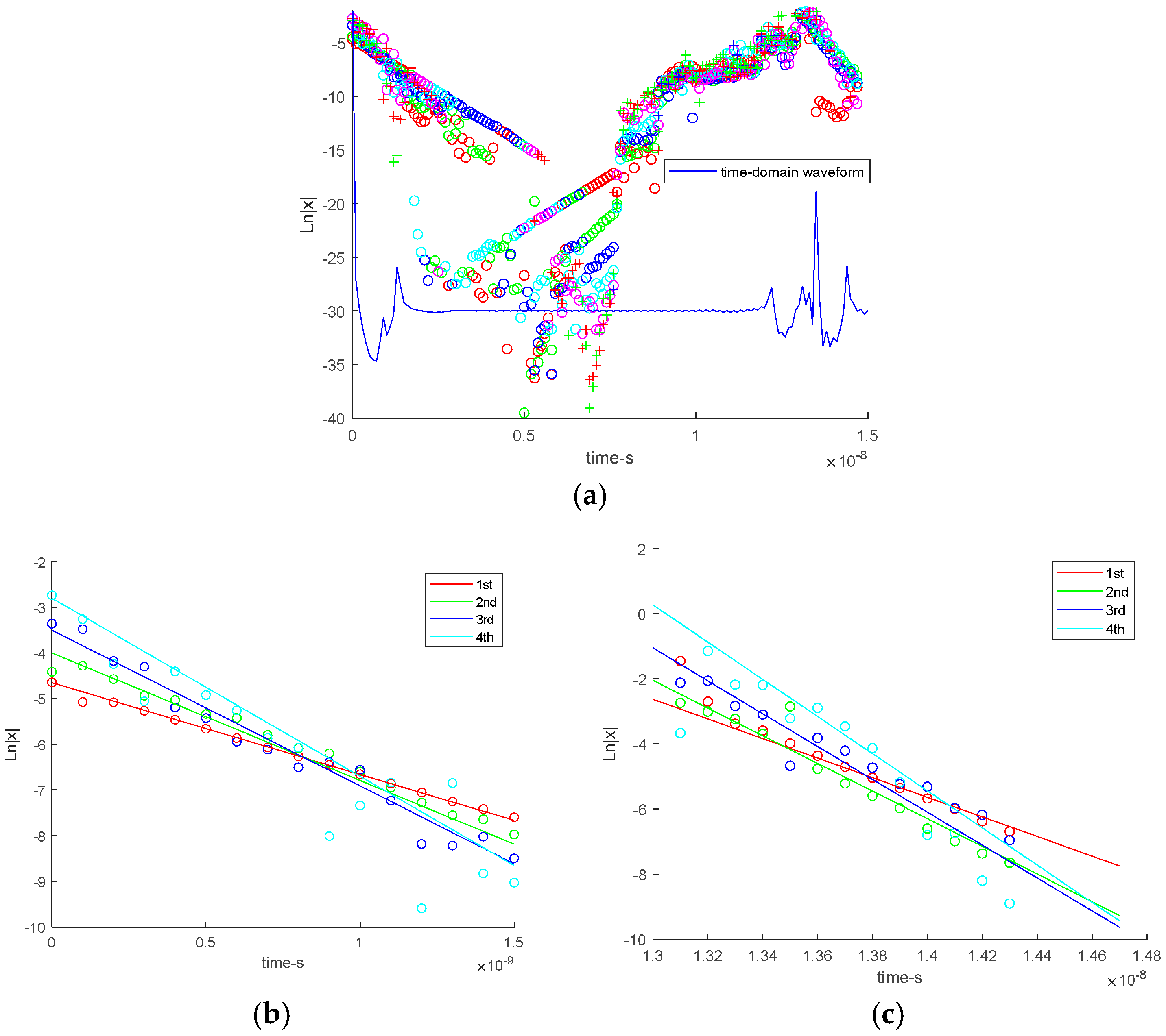
3.2. Extracting the Pole Information
4. Discussion
5. Conclusions
Author Contributions
Funding
Data Availability Statement
Conflicts of Interest
References
- Li, S.; Hargrave, C.O.; Lui, H.S. Resonance-based Radar Target Classification using the Matrix Pencil Method and the Cauchy Method. In Proceedings of the 2021 IEEE International Symposium on Antennas and Propagation and USNC-URSI Radio Science Meeting (APS/URSI), Singapore, 4–10 December 2021; pp. 1341–1342. [Google Scholar]
- Ma, X.; Zhou, Z.; Liu, K.; Zhang, J.; Raza, W. Poles extraction of underwater targets based on matrix pencil method. IEEE Access 2020, 8, 103007–103019. [Google Scholar] [CrossRef]
- Feng, T.; Yang, J.; Ge, P.; Zhang, S.; Du, Y.; Wang, H. An Improved Pole Extraction Algorithm with Low Signal-to-Noise Ratio. In Proceedings of the 2021 IEEE 4th Advanced Information Management, Communicates, Electronic and Automation Control Conference (IMCEC), Chongqing, China, 18–20 June 2021; Volume 4, pp. 1146–1150. [Google Scholar]
- Baum, C.E. The Singularity Expansion Method Transient Electromagnetic Fields ed LB Felsen; Springer: New York, NY, USA, 1976. [Google Scholar]
- Baum, C.E. On the singularity expansion method for the solution of electromagnetic interaction problems. Interact. Note 1971, 88, 1–111. [Google Scholar]
- Tesche, F. On the analysis of scattering and antenna problems using the singularity expansion technique. IEEE Trans. Antennas Propag. 1973, 21, 53–62. [Google Scholar] [CrossRef]
- Hamidi, R.J.; Livani, H.; Rezaiesarlak, R. Traveling-wave detection technique using short-time matrix pencil method. IEEE Trans. Power Deliv. 2017, 32, 2565–2574. [Google Scholar]
- Dudley, D.G. Progress in identification of electromagnetic systems. IEEE Antennas Propag. Soc. Newsl. 1988, 30, 5–11. [Google Scholar] [CrossRef]
- Sarkar, T.K.; Pereira, O. Using the matrix pencil method to estimate the parameters of a sum of complex exponentials. IEEE Antennas Propag. Mag. 1995, 37, 48–55. [Google Scholar] [CrossRef]
- Brittingham, J.N.; Miller, E.K.; Willows, J.L. Pole extraction from real-frequency information. Proc. IEEE 1980, 68, 263–273. [Google Scholar] [CrossRef]
- Wu, X.; Dong, Y.; Yang, Q.; Deng, W. Target Feature Extraction in Narrowband Mode. In Proceedings of the 2020 14th European Conference on Antennas and Propagation (EuCAP), Copenhagen, Denmark, 15–20 March 2020; pp. 1–4. [Google Scholar]
- Anuradha, S.; Balakrishnan, J. Resonance based discrimination of targets with minor structural variations. In Proceedings of the 2016 Asia-Pacific Microwave Conference (APMC), New Delhi, India, 5–9 December 2016; pp. 1–5. [Google Scholar]
- Deng, Z.; Zhang, T.; Li, N.; Zhang, C.; Si, W. Pole Extraction of Radar Target in Resonant Region Based on Sliding-Window Matrix Pencil Method. Wirel. Commun. Mob. Comput. 2022, 2022, 1539056. [Google Scholar] [CrossRef]
- Rezaiesarlak, R.; Manteghi, M. Accurate extraction of early-/late-time responses using short-time matrix pencil method for transient analysis of scatterers. IEEE Trans. Antennas Propag. 2015, 63, 4995–5002. [Google Scholar] [CrossRef]
- Lee, W.; Sarkar, T.K.; Moon, H.; Brown, L. Detection and identification using natural frequency of the perfect electrically conducting (PEC) sphere in the frequency and time domain. In Proceedings of the 2011 IEEE International Symposium on Antennas and Propagation (APSURSI), Spokane, WA, USA, 3–8 July 2011; pp. 2334–2337. [Google Scholar]
- Bhattacharyya, N.; Siddiqui, J.Y.; Antar, Y.M. Object Identification With Minimal Precomputed Library Using Physical Aspect Of Singularity Expansion Method. IEEE Antennas Wirel. Propag. Lett. 2022, 22, 883–887. [Google Scholar] [CrossRef]
- Bhattacharyya, N.; Siddiqui, J.Y. Singularity Expansion Method in Radar Multimodal Signal Processing and Antenna Characterization. In Intelligent Multi-Modal Data Processing; Wiley Online Library: Hoboken, NJ, USA, 2021; pp. 231–247. [Google Scholar]
- Liu, X.; Li, J.; Zhu, Y.; Zhang, S. Scattering characteristic extraction and recovery for multiple targets based on time frequency analysis. Appl. Comput. Electromagn. Soc. J.(ACES) 2020, 35, 962–970. [Google Scholar] [CrossRef]
- Li, S.; Yang, C.; Gu, P.; He, Z.; Chen, R. Fast Parameter Estimation by Using Matrix Pencil Method. In Proceedings of the 2021 Photonics & Electromagnetics Research Symposium (PIERS), Hangzhou, China, 21–25 November 2021; pp. 43–48. [Google Scholar]
- Sun, Y.; Xiong, H.; Tan DK, P.; Han, T.X.; Du, R.; Yang, X.; Ye, T.T. Moving target localization and activity/gesture recognition for indoor radio frequency sensing applications. IEEE Sens. J. 2021, 21, 24318–24326. [Google Scholar] [CrossRef]
- Chauveau, J.; De Beaucoudrey, N.; Saillard, J. Characterization of radar targets in resonance domain with a reduced number of natural poles. In Proceedings of the European Radar Conference, EURAD 2005, Paris, France, 3–4 October 2005; pp. 69–72. [Google Scholar]
- Wang, Y.; Lei, M.; Zhang, Y.; Zhao, H. A High Precision Ballistic Target Recognition Framework Using Multi-Subband Fusion. In Proceedings of the 2023 International Applied Computational Electromagnetics Society Symposium (ACES-China), Hangzhou, China, 15–18 August 2023; pp. 1–3. [Google Scholar]
- Sathe, P.; Bhattacharya, A. Automatic object discrimination based on natural resonant features of dielectric coated object. IEEE Trans. Antennas Propag. 2022, 71, 2039–2044. [Google Scholar] [CrossRef]
- Yang, J.; Sarkar, T.K. Interpolation/extrapolation of radar cross-section (RCS) data in the frequency domain using the Cauchy method. IEEE Trans. Antennas Propag. 2007, 55, 2844–2851. [Google Scholar] [CrossRef]


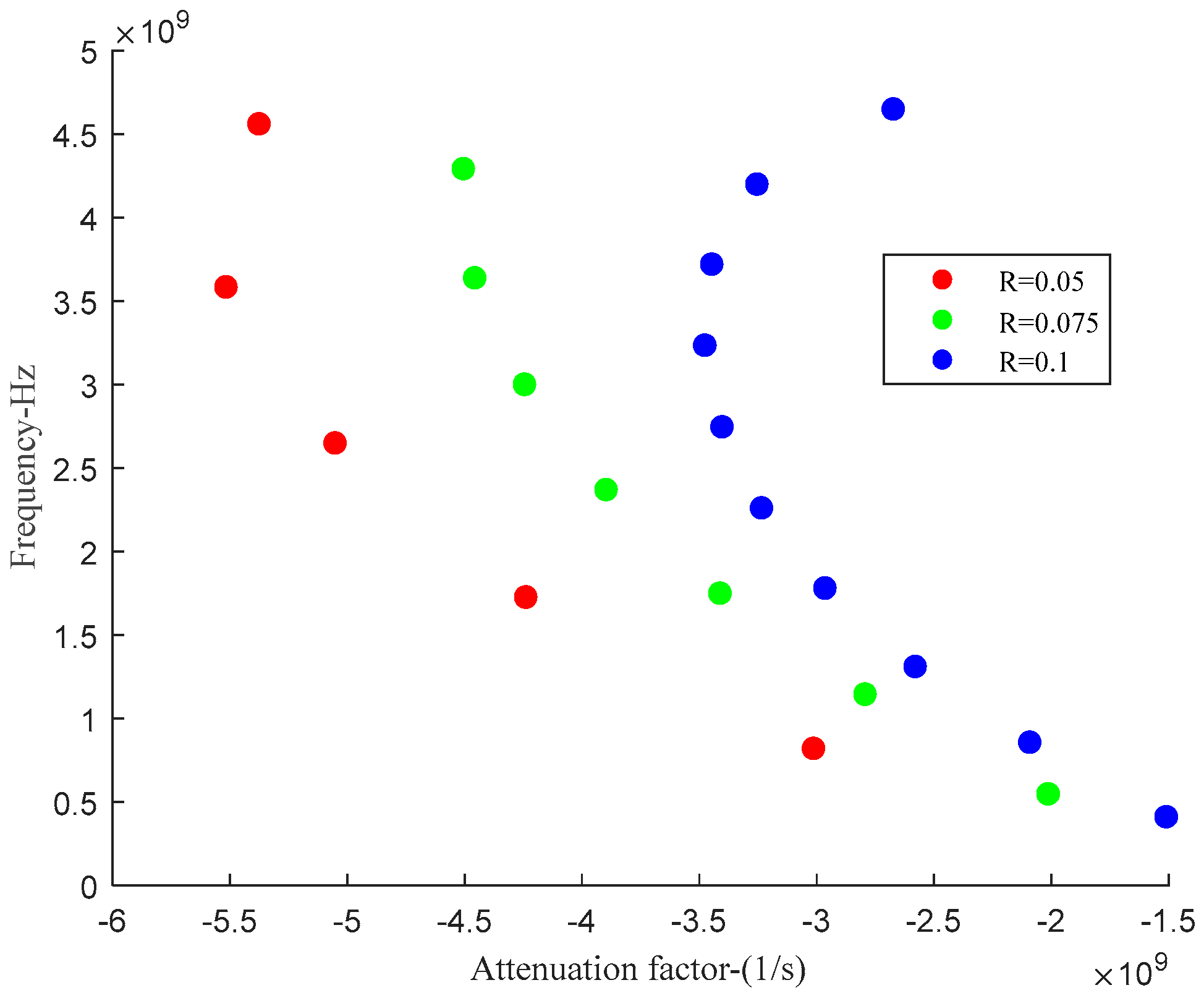
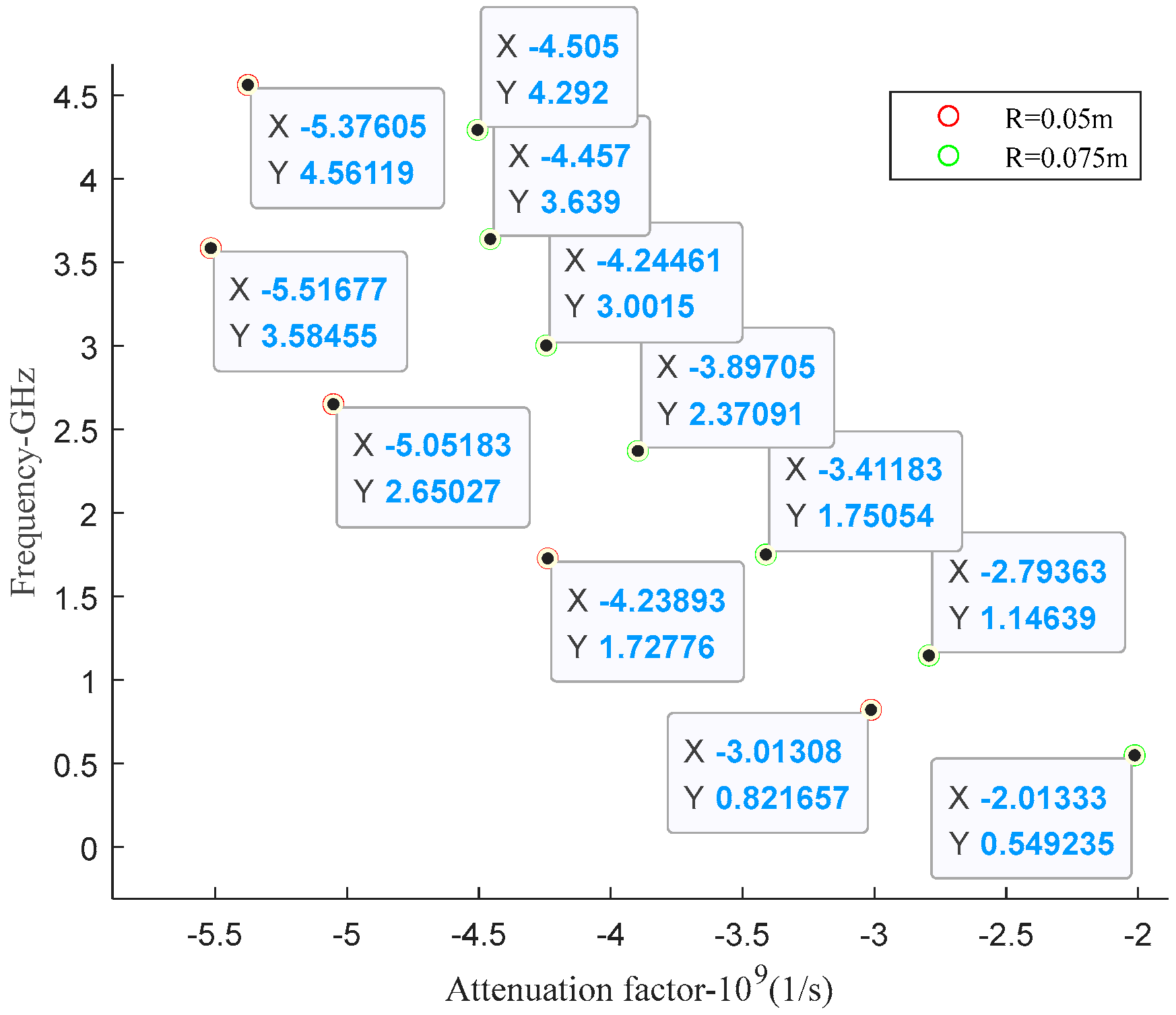
| Radii | R = 0.05 | R = 0.075 | R = 0.1 |
|---|---|---|---|
| 1st | (−3.01, 0.82) | (−2.01, 0.55) | (−1.51, 0.41) |
| 2nd | (−4.24, 1.73) | (−2.79, 1.15) | (−2.09, 0.86) |
| 3rd | (−5.05, 2.65) | (−3.41, 1.75) | (−2.58, 1.31) |
| 4th | (−5.52, 3.59) | (−3.90, 2.37) | (−2.96, 1.78) |
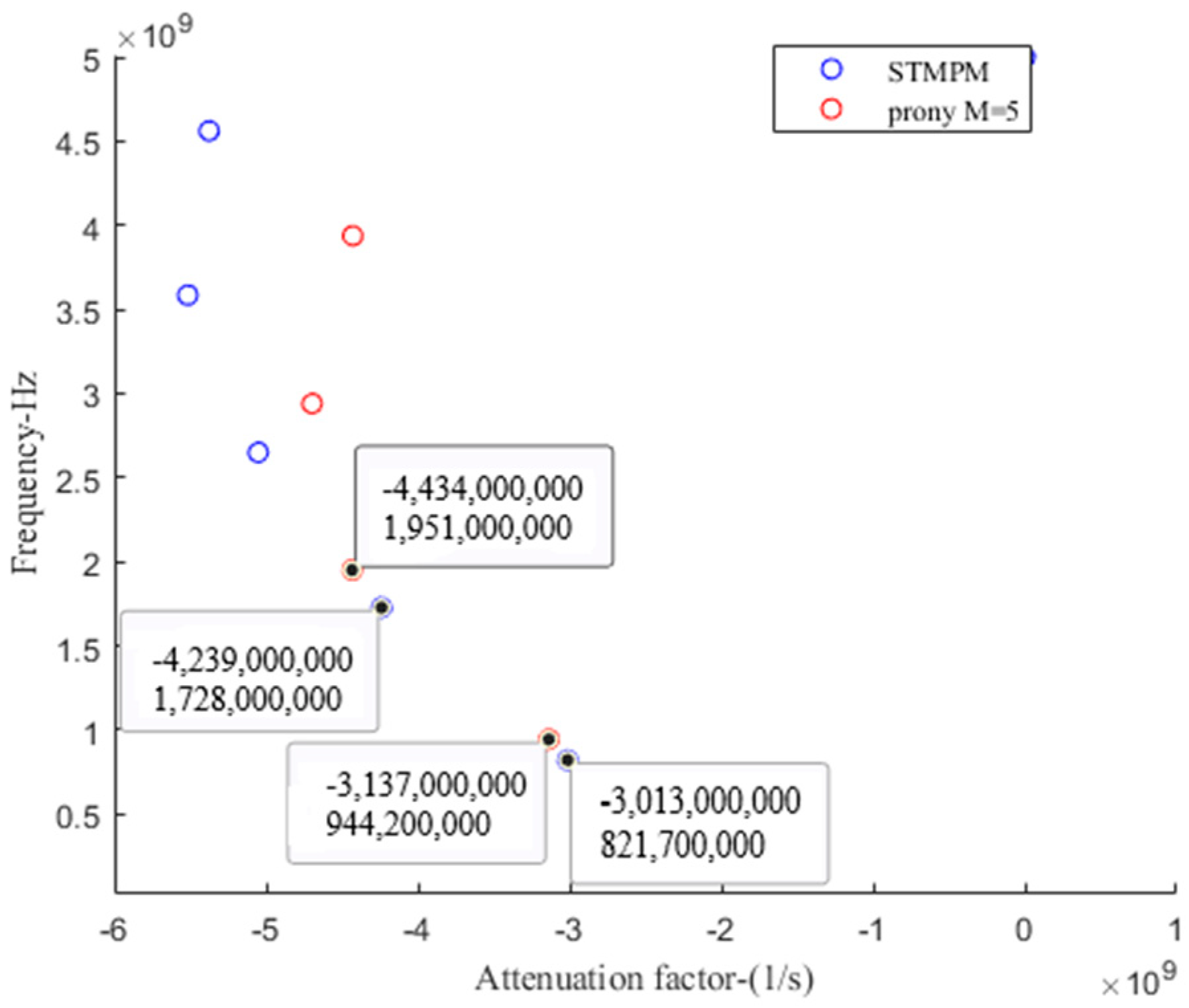
| Poles | STMPM | Prony (M = 5) | Deviation |
|---|---|---|---|
| 1st | (−3.01, 0.82) | (−3.14, 0.94) | 0.3% |
| 2nd | (−4.24, 1.73) | (−4.43, 1.95) | 0.4% |
| 3rd | (−5.05, 2.65) | (−4.70, 2.94) | 0.6% |
| 4th | (−5.52, 3.59) | (−4.43, 3.94) | 2% |
Disclaimer/Publisher’s Note: The statements, opinions and data contained in all publications are solely those of the individual author(s) and contributor(s) and not of MDPI and/or the editor(s). MDPI and/or the editor(s) disclaim responsibility for any injury to people or property resulting from any ideas, methods, instructions or products referred to in the content. |
© 2025 by the authors. Licensee MDPI, Basel, Switzerland. This article is an open access article distributed under the terms and conditions of the Creative Commons Attribution (CC BY) license (https://creativecommons.org/licenses/by/4.0/).
Share and Cite
Zhao, Z.; Wu, X.; Deng, W. Multi-Object Feature Extraction in Resonance Region Based on Short-Time Matrix Pencil Method. Remote Sens. 2025, 17, 1429. https://doi.org/10.3390/rs17081429
Zhao Z, Wu X, Deng W. Multi-Object Feature Extraction in Resonance Region Based on Short-Time Matrix Pencil Method. Remote Sensing. 2025; 17(8):1429. https://doi.org/10.3390/rs17081429
Chicago/Turabian StyleZhao, Zeying, Xiaochuan Wu, and Weibo Deng. 2025. "Multi-Object Feature Extraction in Resonance Region Based on Short-Time Matrix Pencil Method" Remote Sensing 17, no. 8: 1429. https://doi.org/10.3390/rs17081429
APA StyleZhao, Z., Wu, X., & Deng, W. (2025). Multi-Object Feature Extraction in Resonance Region Based on Short-Time Matrix Pencil Method. Remote Sensing, 17(8), 1429. https://doi.org/10.3390/rs17081429