
Modeling Worldwide Tree Biodiversity Using Canopy Structure Metrics from Global Ecosystem Dynamics Investigation Data


Abstract
:1. Introduction
2. Materials and Methods
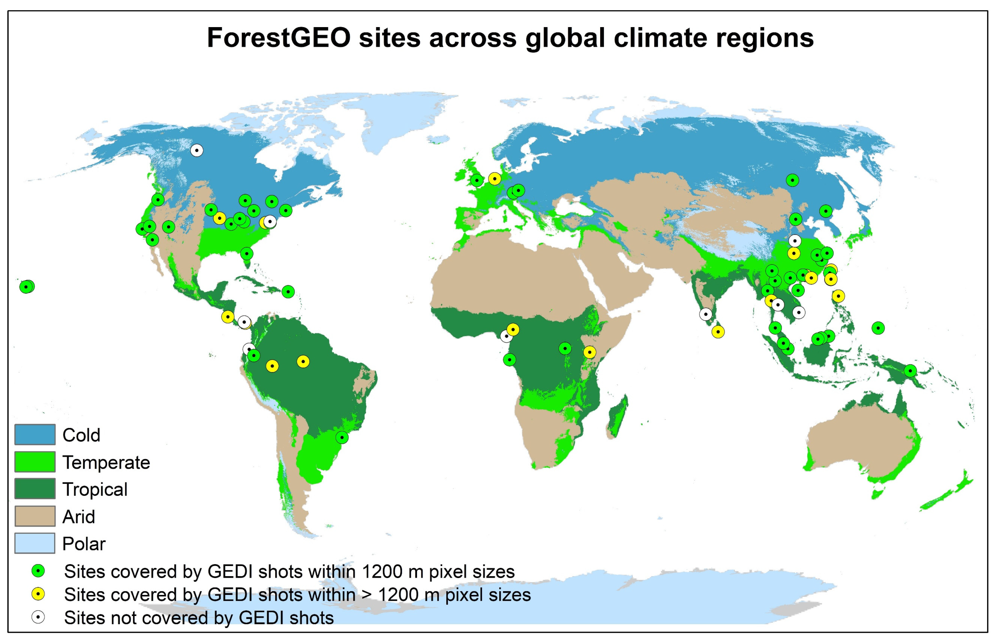
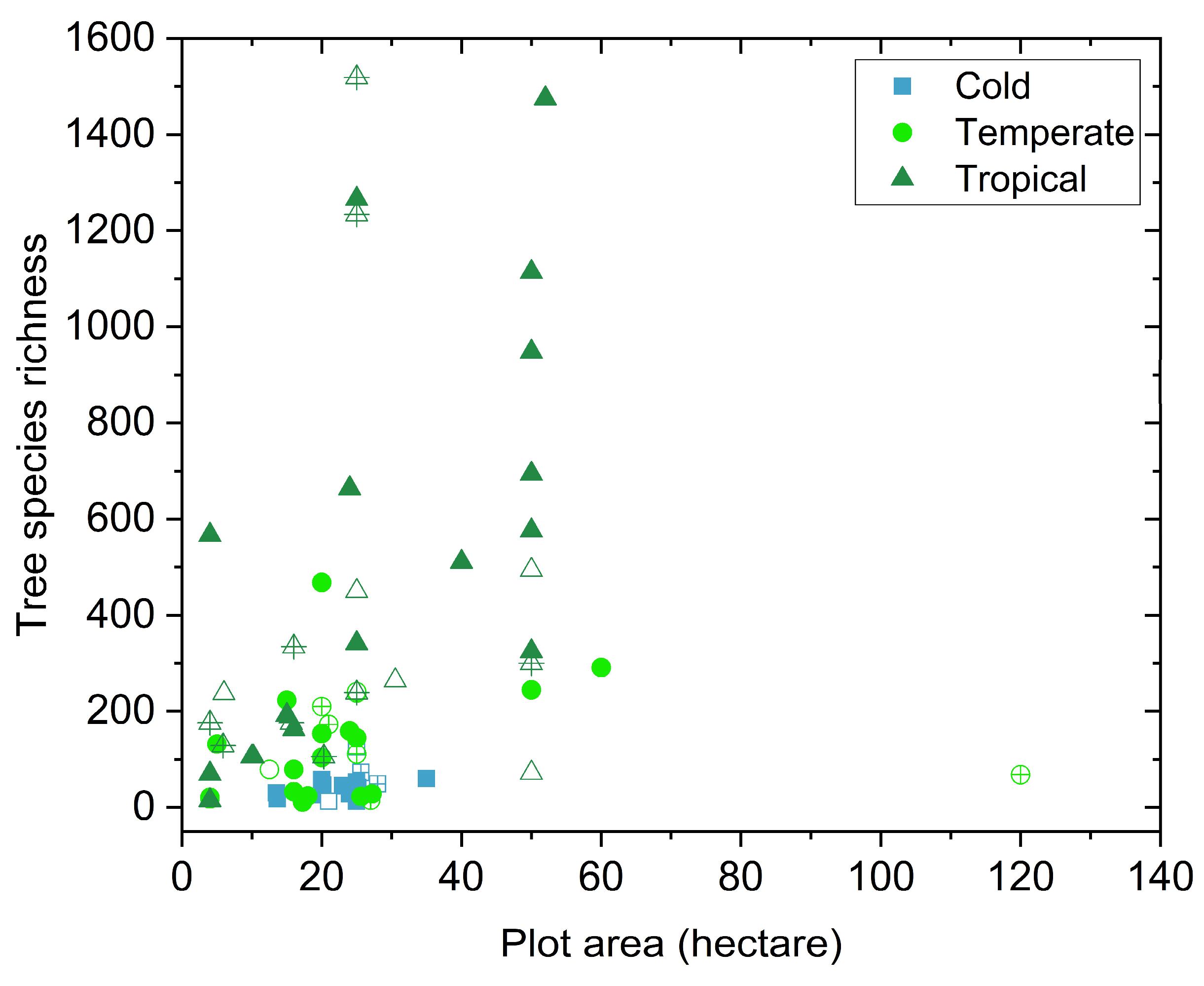
2.1. ForestGEO Data
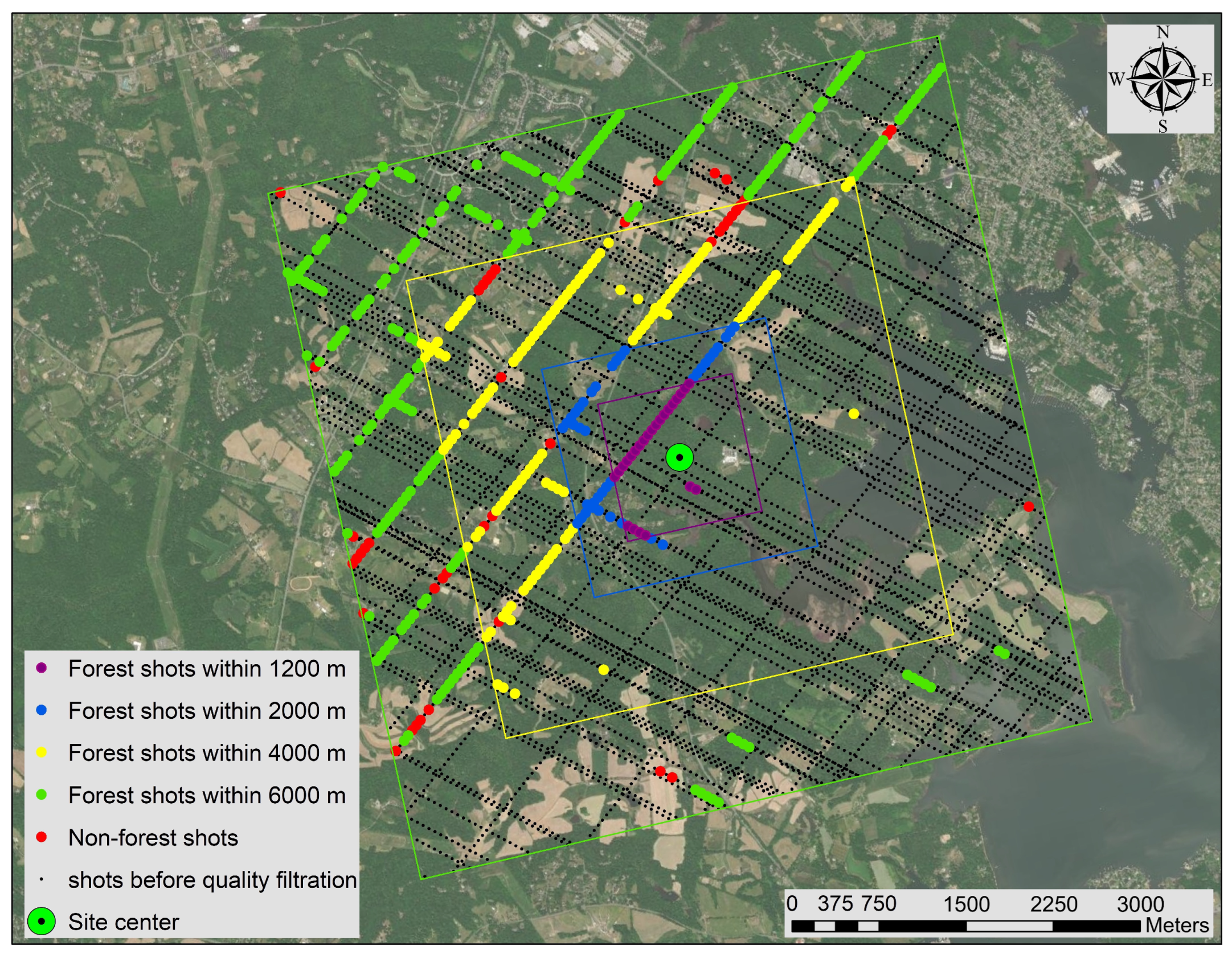
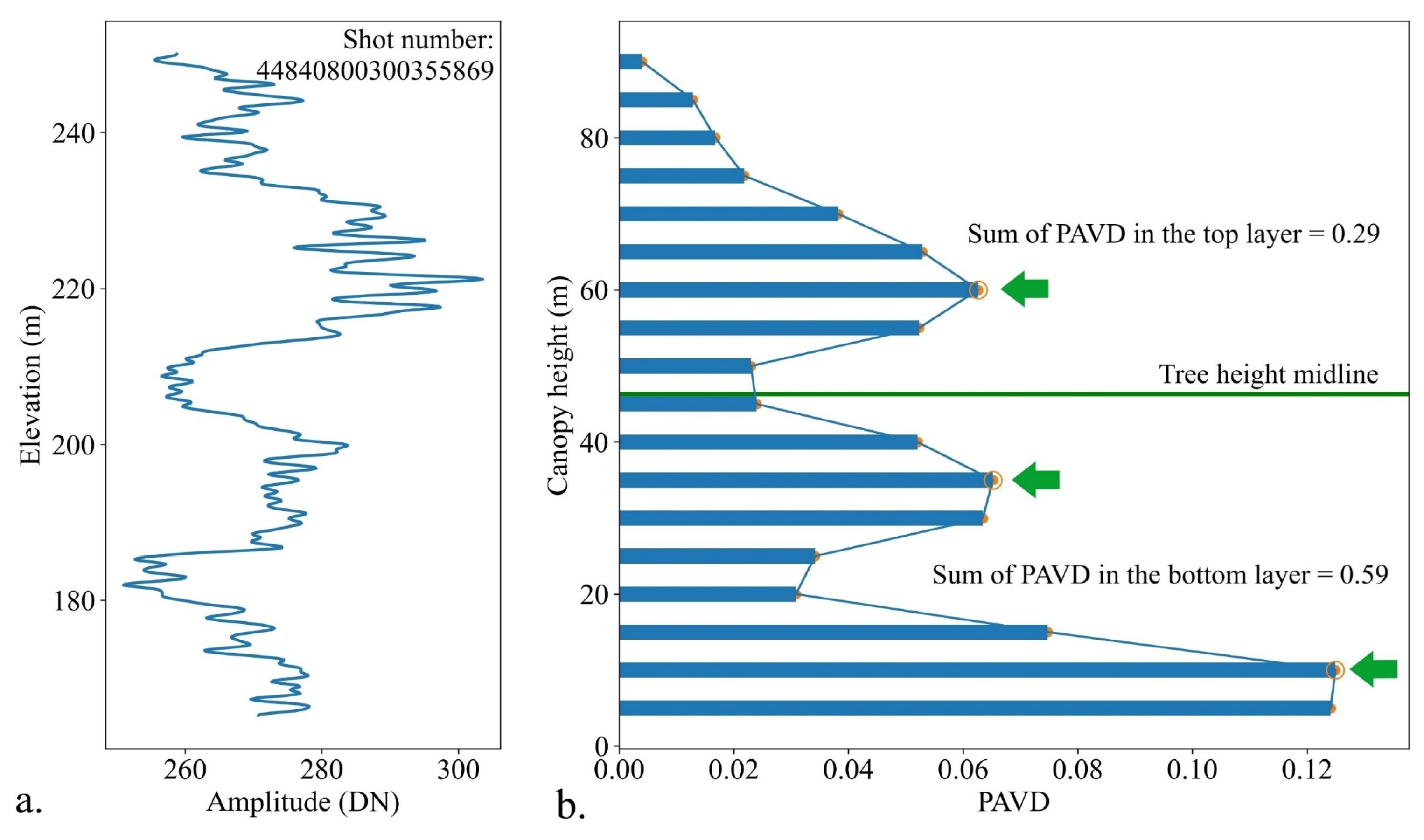
2.2. GEDI Data
2.3. Spectral Vegetation Metrics
2.4. Feature Selection
2.5. Tree Species Richness Model Using the ForestGEO Dataset Across Spatial Scales
3. Results
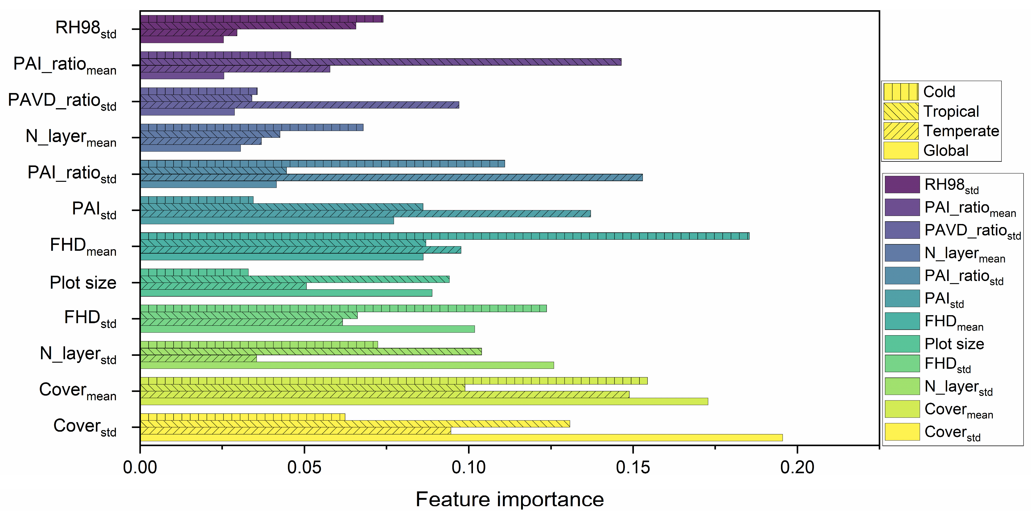
3.1. Feature Correlation and Selection
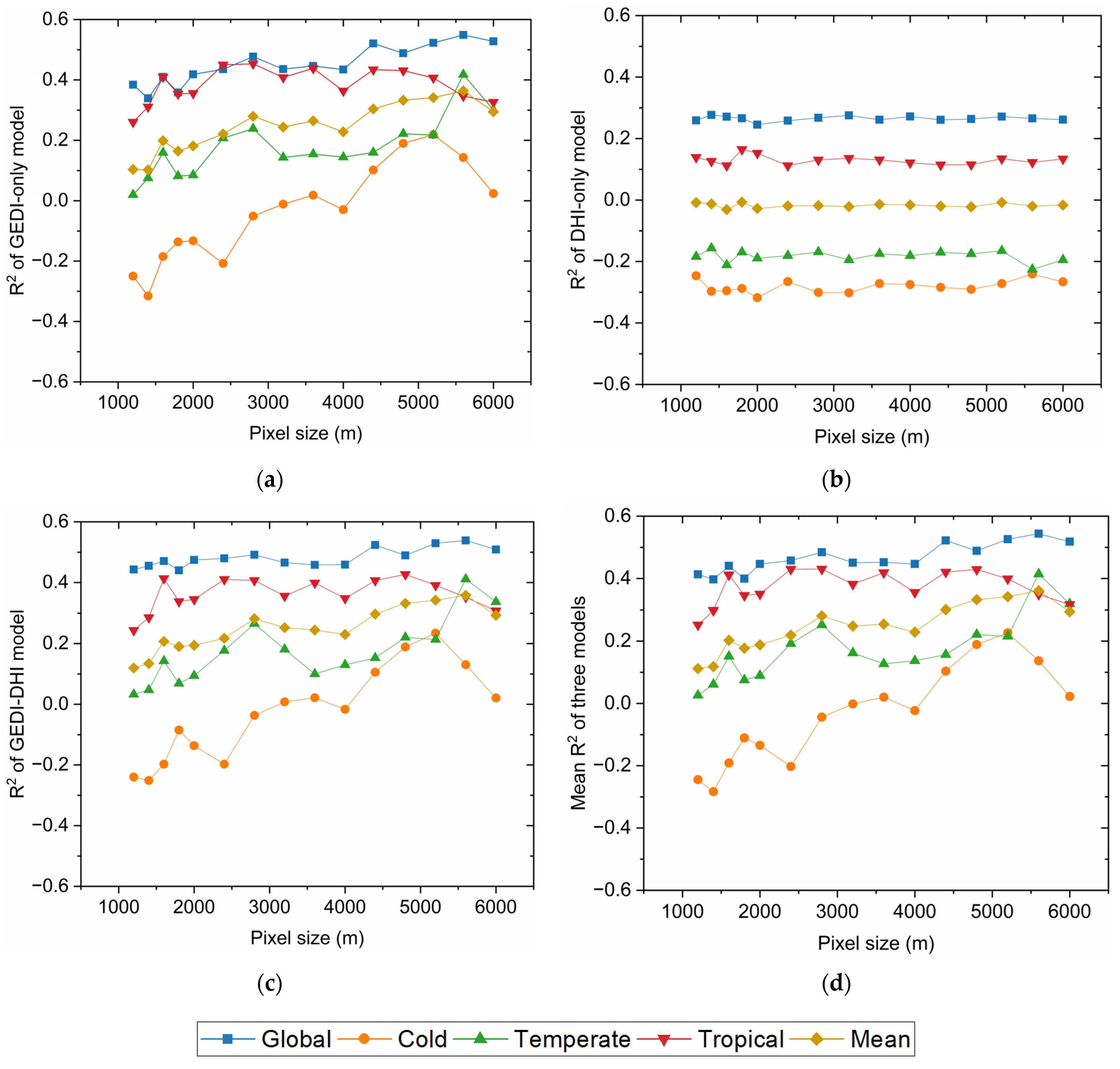
3.2. Optimized Universal Hyperparameter and Pixel Size Determination
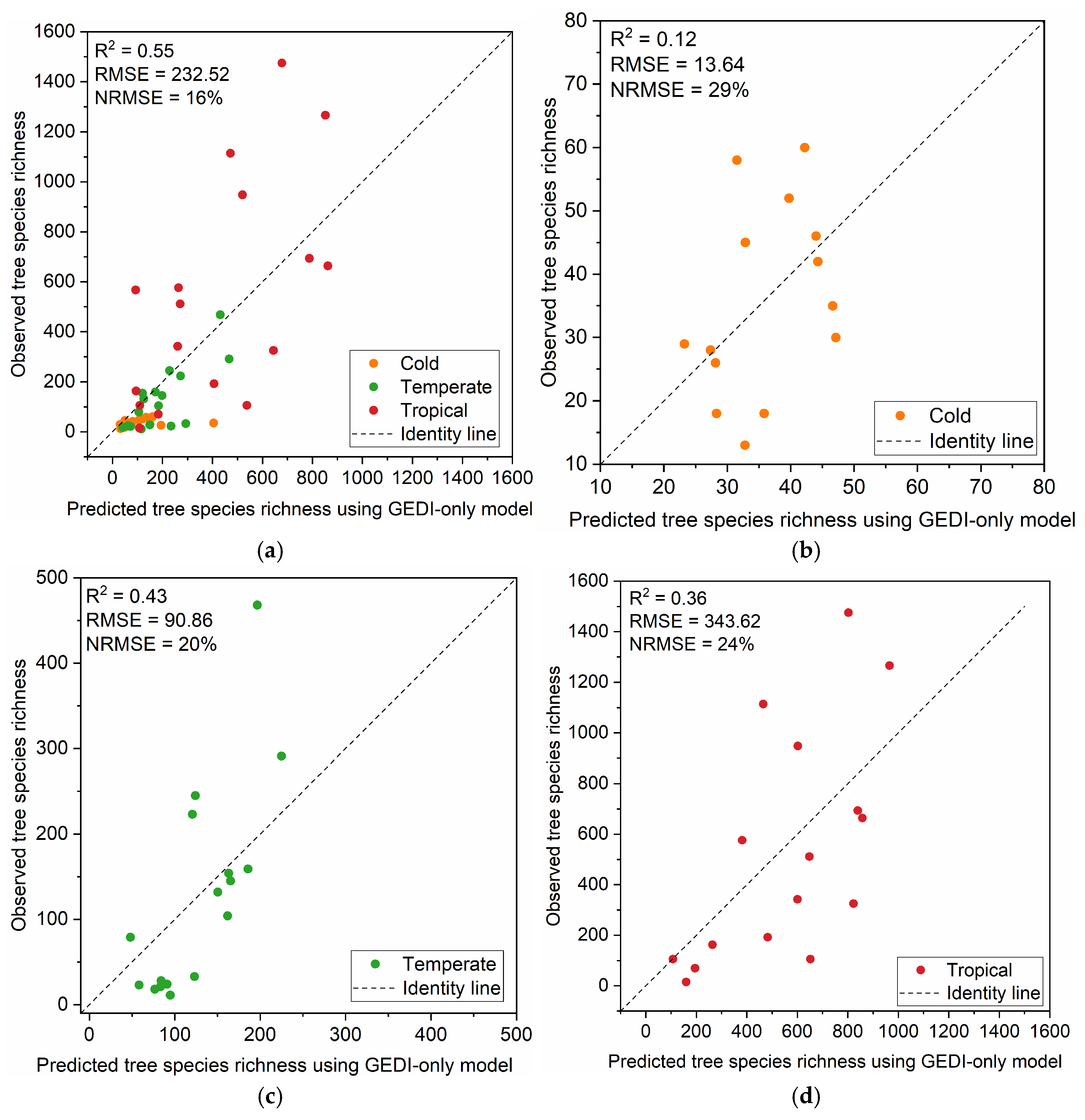
3.3. Model Performance and Comparison
4. Discussion
4.1. Model Performance
4.2. Data Source
4.3. Future Work
5. Conclusions
Supplementary Materials
Author Contributions
Funding
Data Availability Statement
Conflicts of Interest
Appendix A

| Parameter | Description | Assigned Values |
|---|---|---|
| n_estimators | The number of trees in the forest. | 10, 50, 100, 300, 500, 700, 900, 1100, 1300, 1500, 1700, 1900, 2100 |
| max_depth | The maximum depth of the tree. If None, then split until nodes cannot expand further and until all leaves contain less than min_samples_split samples. | 2, 4, 6, 8, 10, 20, None |
| max_features | The number of features to consider when looking for the best split. | “sqrt”, “log2”, “auto” |

References
- Marín, A.I.; Abdul Malak, D.; Bastrup-Birk, A.; Chirici, G.; Barbati, A.; Kleeschulte, S. Mapping forest condition in Europe: Methodological developments in support to forest biodiversity assessments. Ecol. Indic. 2021, 128, 107839. [Google Scholar] [CrossRef]
- Taye, F.A.; Folkersen, M.V.; Fleming, C.M.; Buckwell, A.; Mackey, B.; Diwakar, K.C.; Le, D.; Hasan, S.; Ange, C.S. The economic values of global forest ecosystem services: A meta-analysis. Ecol. Econ. 2021, 189, 107145. [Google Scholar] [CrossRef]
- Wang, R.; Gamon, J.A. Remote sensing of terrestrial plant biodiversity. Remote Sens. Environ. 2019, 231, 111218. [Google Scholar] [CrossRef]
- Isbell, F.; Craven, D.; Connolly, J.; Loreau, M.; Schmid, B.; Beierkuhnlein, C.; Bezemer, T.M.; Bonin, C.; Bruelheide, H.; de Luca, E.; et al. Biodiversity increases the resistance of ecosystem productivity to climate extremes. Nature 2015, 526, 574–577. [Google Scholar] [CrossRef]
- Schnabel, F.; Liu, X.; Kunz, M.; Barry, K.E.; Bongers, F.J.; Bruelheide, H.; Fichtner, A.; Härdtle, W.; Li, S.; Pfaff, C.-T.; et al. Species richness stabilizes productivity via asynchrony and drought-tolerance diversity in a large-scale tree biodiversity experiment. Sci. Adv. 2021, 7, eabk1643. [Google Scholar] [CrossRef]
- Scherer-Lorenzen, M.; Luis Bonilla, J.; Potvin, C. Tree species richness affects litter production and decomposition rates in a tropical biodiversity experiment. Oikos 2007, 116, 2108–2124. [Google Scholar] [CrossRef]
- Tuanmu, M.N.; Jetz, W. A global, remote sensing-based characterization of terrestrial habitat heterogeneity for biodiversity and ecosystem modelling. Glob. Ecol. Biogeogr. 2015, 24, 1329–1339. [Google Scholar] [CrossRef]
- Gotelli, N.J.; Colwell, R.K. Quantifying biodiversity: Procedures and pitfalls in the measurement and comparison of species richness. Ecol. Lett. 2001, 4, 379–391. [Google Scholar] [CrossRef]
- Ricklefs, R.E.; He, F. Region effects influence local tree species diversity. Proc. Natl. Acad. Sci. USA 2016, 113, 674–679. [Google Scholar] [CrossRef]
- Cazzolla Gatti, R.; Reich, P.B.; Gamarra, J.G.; Crowther, T.; Hui, C.; Morera, A.; Bastin, J.-F.; De-Miguel, S.; Nabuurs, G.-J.; Svenning, J.-C. The number of tree species on Earth. Proc. Natl. Acad. Sci. USA 2022, 119, e2115329119. [Google Scholar] [CrossRef]
- Secretariat of the Convention on Biological Diversity. Global Biodiversity Outlook 5; Convention on Biological Diversity: Montreal, QC, Canada, 2020. [Google Scholar]
- Xu, H.; Cao, Y.; Yu, D.; Cao, M.; He, Y.; Gill, M.; Pereira, H.M. Ensuring effective implementation of the post-2020 global biodiversity targets. Nat. Ecol. Evol. 2021, 5, 411–418. [Google Scholar] [CrossRef]
- Steane, D.A.; Potts, B.M.; McLean, E.; Prober, S.M.; Stock, W.D.; Vaillancourt, R.E.; Byrne, M. Genome-wide scans detect adaptation to aridity in a widespread forest tree species. Mol. Ecol. 2014, 23, 2500–2513. [Google Scholar] [CrossRef]
- Meyer, L.; Diniz-Filho, J.A.F.; Lohmann, L.G.; Hortal, J.; Barreto, E.; Rangel, T.; Kissling, W.D. Canopy height explains species richness in the largest clade of Neotropical lianas. Glob. Ecol. Biogeogr. 2020, 29, 26–37. [Google Scholar] [CrossRef]
- Stein, A.; Gerstner, K.; Kreft, H. Environmental heterogeneity as a universal driver of species richness across taxa, biomes and spatial scales. Ecol. Lett. 2014, 17, 866–880. [Google Scholar] [CrossRef]
- Ollinger, S.V. Sources of variability in canopy reflectance and the convergent properties of plants. New Phytol. 2011, 189, 375–394. [Google Scholar] [CrossRef]
- Bergen, K.; Goetz, S.; Dubayah, R.; Henebry, G.; Hunsaker, C.; Imhoff, M.; Nelson, R.; Parker, G.; Radeloff, V. Remote sensing of vegetation 3-D structure for biodiversity and habitat: Review and implications for lidar and radar spaceborne missions. J. Geophys. Res. Biogeosciences 2009, 114, G00E06. [Google Scholar] [CrossRef]
- Lopatin, J.; Dolos, K.; Hernández, H.; Galleguillos, M.; Fassnacht, F. Comparing generalized linear models and random forest to model vascular plant species richness using LiDAR data in a natural forest in central Chile. Remote Sens. Environ. 2016, 173, 200–210. [Google Scholar] [CrossRef]
- Hill, S.L.L.; Arnell, A.; Maney, C.; Butchart, S.H.M.; Hilton-Taylor, C.; Ciciarelli, C.; Davis, C.; Dinerstein, E.; Purvis, A.; Burgess, N.D. Measuring Forest Biodiversity Status and Changes Globally. Front. For. Glob. Change 2019, 2, 70. [Google Scholar] [CrossRef]
- Schiefer, F.; Kattenborn, T.; Frick, A.; Frey, J.; Schall, P.; Koch, B.; Schmidtlein, S. Mapping forest tree species in high resolution UAV-based RGB-imagery by means of convolutional neural networks. ISPRS J. Photogramm. Remote Sens. 2020, 170, 205–215. [Google Scholar] [CrossRef]
- Huang, S.; Tang, L.; Hupy, J.P.; Wang, Y.; Shao, G. A commentary review on the use of normalized difference vegetation index (NDVI) in the era of popular remote sensing. J. For. Res. 2021, 32, 1–6. [Google Scholar] [CrossRef]
- Pouteau, R.; Gillespie, T.W.; Birnbaum, P. Predicting Tropical Tree Species Richness from Normalized Difference Vegetation Index Time Series: The Devil Is Perhaps Not in the Detail. Remote Sens. 2018, 10, 698. [Google Scholar] [CrossRef]
- Arekhi, M.; Yılmaz, O.Y.; Yılmaz, H.; Akyüz, Y.F. Can tree species diversity be assessed with Landsat data in a temperate forest? Environ. Monit. Assess. 2017, 189, 586. [Google Scholar] [CrossRef]
- Walter, J.A.; Stovall, A.E.L.; Atkins, J.W. Vegetation structural complexity and biodiversity in the Great Smoky Mountains. Ecosphere 2021, 12, e03390. [Google Scholar] [CrossRef]
- Vogeler, J.C.; Cohen, W.B. A review of the role of active remote sensing and data fusion for characterizing forest in wildlife habitat models. Rev. De Teledetección 2016, 45, 1–14. [Google Scholar] [CrossRef]
- Almeida, D.R.A.d.; Broadbent, E.N.; Ferreira, M.P.; Meli, P.; Zambrano, A.M.A.; Gorgens, E.B.; Resende, A.F.; de Almeida, C.T.; do Amaral, C.H.; Corte, A.P.D.; et al. Monitoring restored tropical forest diversity and structure through UAV-borne hyperspectral and lidar fusion. Remote Sens. Environ. 2021, 264, 112582. [Google Scholar] [CrossRef]
- Fagua, J.C.; Jantz, P.; Burns, P.; Massey, R.; Buitrago, J.Y.; Saatchi, S.; Hakkenberg, C.; Goetz, S.J. Mapping tree diversity in the tropical forest region of Chocó-Colombia. Environ. Res. Lett. 2021, 16, 054024. [Google Scholar] [CrossRef]
- Madonsela, S.; Cho, M.A.; Ramoelo, A.; Mutanga, O.; Naidoo, L. Estimating tree species diversity in the savannah using NDVI and woody canopy cover. Int. J. Appl. Earth Obs. Geoinf. 2018, 66, 106–115. [Google Scholar] [CrossRef]
- Schmidt-Traub, G. National climate and biodiversity strategies are hamstrung by a lack of maps. Nat. Ecol. Evol. 2021, 5, 1325–1327. [Google Scholar] [CrossRef]
- Keil, P.; Chase, J.M. Global patterns and drivers of tree diversity integrated across a continuum of spatial grains. Nat. Ecol. Evol. 2019, 3, 390–399. [Google Scholar] [CrossRef]
- Dubayah, R.; Blair, J.B.; Goetz, S.; Fatoyinbo, L.; Hansen, M.; Healey, S.; Hofton, M.; Hurtt, G.; Kellner, J.; Luthcke, S.; et al. The Global Ecosystem Dynamics Investigation: High-resolution laser ranging of the Earth’s forests and topography. Sci. Remote Sens. 2020, 1, 100002. [Google Scholar] [CrossRef]
- Tang, H.; Armston, J. Algorithm Theoretical Basis Document (ATBD) for GEDI L2B Footprint Canopy Cover and Vertical Profile Metrics; Goddard Space Flight Center: Greenbelt, MD, USA, 2019. [Google Scholar]
- Marselis, S.M.; Tang, H.; Armston, J.; Abernethy, K.; Alonso, A.; Barbier, N.; Bissiengou, P.; Jeffery, K.; Kenfack, D.; Labrière, N.; et al. Exploring the relation between remotely sensed vertical canopy structure and tree species diversity in Gabon. Environ. Res. Lett. 2019, 14, 094013. [Google Scholar] [CrossRef]
- Marselis, S.M.; Abernethy, K.; Alonso, A.; Armston, J.; Baker, T.R.; Bastin, J.-F.; Bogaert, J.; Boyd, D.S.; Boeckx, P.; Burslem, D.F.R.P.; et al. Evaluating the potential of full-waveform lidar for mapping pan-tropical tree species richness. Glob. Ecol. Biogeogr. 2020, 29, 1799–1816. [Google Scholar] [CrossRef]
- Marselis, S.M.; Keil, P.; Chase, J.M.; Dubayah, R. The use of GEDI canopy structure for explaining variation in tree species richness in natural forests. Environ. Res. Lett. 2022, 17, 045003. [Google Scholar] [CrossRef]
- Davies, S.J.; Abiem, I.; Abu Salim, K.; Aguilar, S.; Allen, D.; Alonso, A.; Anderson-Teixeira, K.; Andrade, A.; Arellano, G.; Ashton, P.S.; et al. ForestGEO: Understanding forest diversity and dynamics through a global observatory network. Biol. Conserv. 2021, 253, 108907. [Google Scholar] [CrossRef]
- Beck, H.E.; Zimmermann, N.E.; McVicar, T.R.; Vergopolan, N.; Berg, A.; Wood, E.F. Present and future Köppen-Geiger climate classification maps at 1-km resolution. Sci. Data 2018, 5, 180214. [Google Scholar] [CrossRef]
- Jantz, S.M.; Barker, B.; Brooks, T.M.; Chini, L.P.; Huang, Q.; Moore, R.M.; Noel, J.; Hurtt, G.C. Future habitat loss and extinctions driven by land-use change in biodiversity hotspots under four scenarios of climate-change mitigation. Conserv. Biol. 2015, 29, 1122–1131. [Google Scholar] [CrossRef]
- Lomolino, M.V. The species-area relationship: New challenges for an old pattern. Prog. Phys. Geogr. Earth Environ. 2001, 25, 1–21. [Google Scholar] [CrossRef]
- Buchhorn, M.; Smets, B.; Bertels, L.; De Roo, B.; Lesiv, M.; Tsendbazar, N.E.; Tarko, A.J. Copernicus Global Land Service: Land Cover 100m: Version 3 Globe 2015-2019: Product User Manual (Dataset v3.0, doc issue 3.4). Zenodo. [CrossRef]
- Jutz, S.; Milagro-Pérez, M. Copernicus: The European Earth Observation programme. Rev. De Teledetección 2020, 56, V–XI. [Google Scholar] [CrossRef]
- Buchhorn, M.; Lesiv, M.; Tsendbazar, N.-E.; Herold, M.; Bertels, L.; Smets, B. Copernicus Global Land Cover Layers—Collection 2. Remote Sens. 2020, 12, 1044. [Google Scholar] [CrossRef]
- Xu, J.; Farwell, L.; Radeloff, V.C.; Luther, D.; Songer, M.; Cooper, W.J.; Huang, Q. Avian diversity across guilds in North America versus vegetation structure as measured by the Global Ecosystem Dynamics Investigation (GEDI). Remote Sens. Environ. 2024, 315, 114446. [Google Scholar] [CrossRef]
- Whitehurst, A.S.; Swatantran, A.; Blair, J.B.; Hofton, M.A.; Dubayah, R. Characterization of Canopy Layering in Forested Ecosystems Using Full Waveform Lidar. Remote Sens. 2013, 5, 2014–2036. [Google Scholar] [CrossRef]
- Radeloff, V.C.; Dubinin, M.; Coops, N.C.; Allen, A.M.; Brooks, T.M.; Clayton, M.K.; Costa, G.C.; Graham, C.H.; Helmers, D.P.; Ives, A.R.; et al. The Dynamic Habitat Indices (DHIs) from MODIS and global biodiversity. Remote Sens. Environ. 2019, 222, 204–214. [Google Scholar] [CrossRef]
- Chandrashekar, G.; Sahin, F. A survey on feature selection methods. Comput. Electr. Eng. 2014, 40, 16–28. [Google Scholar] [CrossRef]
- Schulz, D.; Yin, H.; Tischbein, B.; Verleysdonk, S.; Adamou, R.; Kumar, N. Land use mapping using Sentinel-1 and Sentinel-2 time series in a heterogeneous landscape in Niger, Sahel. ISPRS J. Photogramm. Remote Sens. 2021, 178, 97–111. [Google Scholar] [CrossRef]
- Jin, Z.; Azzari, G.; You, C.; Di Tommaso, S.; Aston, S.; Burke, M.; Lobell, D.B. Smallholder maize area and yield mapping at national scales with Google Earth Engine. Remote Sens. Environ. 2019, 228, 115–128. [Google Scholar] [CrossRef]
- Segal, M.R. Machine Learning Benchmarks and Random Forest Regression; UCSF Center for Bioinformatics and Molecular Biostatistics: San Francisco, CA, USA, 2004. [Google Scholar]
- Qi, Y. Random forest for bioinformatics. In Ensemble Machine Learning; Springer: Berlin/Heidelberg, Germany, 2012; pp. 307–323. [Google Scholar]
- Pedregosa, F.; Varoquaux, G.; Gramfort, A.; Michel, V.; Thirion, B.; Grisel, O.; Blondel, M.; Prettenhofer, P.; Weiss, R.; Dubourg, V. Scikit-learn: Machine learning in Python. J. Mach. Learn. Res. 2011, 12, 2825–2830. [Google Scholar]
- Xu, J.; Quackenbush, L.J.; Volk, T.A.; Im, J. Estimation of shrub willow biophysical parameters across time and space from Sentinel-2 and unmanned aerial system (UAS) data. Field Crops Res. 2022, 287, 108655. [Google Scholar] [CrossRef]
- Smithsonian Institution. Smithsonian Institution High Performance Computing Cluster; Smithsonian Institution: Washington, DC, USA, 2020. [Google Scholar]
- Probst, P.; Wright, M.N.; Boulesteix, A.-L. Hyperparameters and tuning strategies for random forest. WIREs Data Min. Knowl. Discov. 2019, 9, e1301. [Google Scholar] [CrossRef]
- Chernick, M.R.; LaBudde, R.A. An Introduction to Bootstrap Methods with Applications to R; John Wiley & Sons: Hoboken, NJ, USA, 2014. [Google Scholar]
- Nakagawa, S.; Schielzeth, H. A general and simple method for obtaining R2 from generalized linear mixed-effects models. Methods Ecol. Evol. 2013, 4, 133–142. [Google Scholar] [CrossRef]
- Fricker, G.A.; Wolf, J.A.; Saatchi, S.S.; Gillespie, T.W. Predicting spatial variations of tree species richness in tropical forests from high-resolution remote sensing. Ecol. Appl. 2015, 25, 1776–1789. [Google Scholar] [CrossRef] [PubMed]
- Chu, H.-J.; Wang, C.-K.; Huang, M.-L.; Lee, C.-C.; Liu, C.-Y.; Lin, C.-C. Effect of point density and interpolation of LiDAR-derived high-resolution DEMs on landscape scarp identification. GIScience Remote Sens. 2014, 51, 731–747. [Google Scholar] [CrossRef]
- LaRue, E.A.; Fahey, R.; Fuson, T.L.; Foster, J.R.; Matthes, J.H.; Krause, K.; Hardiman, B.S. Evaluating the sensitivity of forest structural diversity characterization to LiDAR point density. Ecosphere 2022, 13, e4209. [Google Scholar] [CrossRef]
- Yeboah, D.; Chen, H.Y.; Kingston, S. Tree species richness decreases while species evenness increases with disturbance frequency in a natural boreal forest landscape. Ecol. Evol. 2016, 6, 842–850. [Google Scholar] [CrossRef]
- Simonson, W.D.; Allen, H.D.; Coomes, D.A. Use of an airborne lidar system to model plant species composition and diversity of Mediterranean oak forests. Conserv. Biol. 2012, 26, 840–850. [Google Scholar] [CrossRef]
- Reddy, C.S. Remote sensing of biodiversity: What to measure and monitor from space to species? Biodivers. Conserv. 2021, 30, 2617–2631. [Google Scholar] [CrossRef]
- Skidmore, A.K.; Coops, N.C.; Neinavaz, E.; Ali, A.; Schaepman, M.E.; Paganini, M.; Kissling, W.D.; Vihervaara, P.; Darvishzadeh, R.; Feilhauer, H. Priority list of biodiversity metrics to observe from space. Nat. Ecol. Evol. 2021, 5, 896–906. [Google Scholar] [CrossRef]


| Metric Categories | Metric Name * |
|---|---|
| Plot metrics (1) | Plot Size (ha) |
| GEDI metrics (16) | RH98mean, RH98std, PAImean, PAIstd, Covermean, Coverstd, FHDmean, FHDstd, N_layermean, N_layerstd, PAVD_ratiomean, PAVD_ratiostd, PAI_ratiomean, PAI_ratiostd, Cover_ratiomean, Cover_ratiostd |
| Spectral vegetation metrics (3) | DHIs-NDVIcum, DHIs-NDVImin, DHIs-NDVIvar |
| Response Variable | Models | Predictors |
|---|---|---|
| ForestGEO tree species richness | DHI-only | Plot size + spectral vegetation metrics |
| GEDI-only | Plot size + GEDI metrics | |
| GEDI-DHI | Plot size + GEDI metrics + spectral vegetation metrics |
| Models | n_estimators | max_depth | max_features |
|---|---|---|---|
| DHI only | 300 | 2 | ‘log2’ |
| GEDI only | 500 | 20 | ‘log2 |
| GEDI-DHIs | 700 | 8 | ‘log2’ |
| Model Performance | GEDI-Only | DHI-Only | GEDI-DHIs | ||||||
|---|---|---|---|---|---|---|---|---|---|
| R2 | RMSE | NRMSE | R2 | RMSE | NRMSE | R2 | RMSE | NRMSE | |
| Global | 0.55 | 232.52 | 16% | 0.27 | 295.66 | 20% | 0.54 | 234.30 | 16% |
| Cold | 0.12 | 13.64 | 29% | −0.24 | 16.19 | 34% | 0.13 | 13.59 | 29% |
| Temperate | 0.43 | 90.86 | 20% | −0.23 | 133.68 | 29% | 0.42 | 91.91 | 20% |
| Tropical | 0.36 | 343.62 | 24% | 0.12 | 403.89 | 28% | 0.34 | 349.52 | 24% |
Disclaimer/Publisher’s Note: The statements, opinions and data contained in all publications are solely those of the individual author(s) and contributor(s) and not of MDPI and/or the editor(s). MDPI and/or the editor(s) disclaim responsibility for any injury to people or property resulting from any ideas, methods, instructions or products referred to in the content. |
© 2025 by the authors. Licensee MDPI, Basel, Switzerland. This article is an open access article distributed under the terms and conditions of the Creative Commons Attribution (CC BY) license (https://creativecommons.org/licenses/by/4.0/).
Share and Cite
Xu, J.; Coleman, K.; Radeloff, V.C.; Songer, M.; Huang, Q. Modeling Worldwide Tree Biodiversity Using Canopy Structure Metrics from Global Ecosystem Dynamics Investigation Data. Remote Sens. 2025, 17, 1408. https://doi.org/10.3390/rs17081408
Xu J, Coleman K, Radeloff VC, Songer M, Huang Q. Modeling Worldwide Tree Biodiversity Using Canopy Structure Metrics from Global Ecosystem Dynamics Investigation Data. Remote Sensing. 2025; 17(8):1408. https://doi.org/10.3390/rs17081408
Chicago/Turabian StyleXu, Jin, Kjirsten Coleman, Volker C. Radeloff, Melissa Songer, and Qiongyu Huang. 2025. "Modeling Worldwide Tree Biodiversity Using Canopy Structure Metrics from Global Ecosystem Dynamics Investigation Data" Remote Sensing 17, no. 8: 1408. https://doi.org/10.3390/rs17081408
APA StyleXu, J., Coleman, K., Radeloff, V. C., Songer, M., & Huang, Q. (2025). Modeling Worldwide Tree Biodiversity Using Canopy Structure Metrics from Global Ecosystem Dynamics Investigation Data. Remote Sensing, 17(8), 1408. https://doi.org/10.3390/rs17081408