Abstract
An ecological restoration assessment aims to evaluate whether ecological restoration projects (ERPs) have achieved predefined ecological objectives, such as improving fractional vegetation cover (FVC) and enhancing ecosystem services (ESs), as well as to optimize restoration strategies based on assessment outcomes. Despite recent advancements, current studies still fall short of fully capturing the trade-offs among ESs and identifying the underlying drivers of different vegetation trends. To address these challenges, we applied the Theil–Sen method to delineate vegetation change zones in the Qilian Mountain National Park (QLMNP) between 2000 and 2020, employed bivariate Moran’s I statistics to analyze the trade-offs and synergies among four ESs within these zones, including carbon sequestration (CS), soil conservation (SC), water conservation (WC), and biodiversity maintenance (BIO), and utilized a spatial random forest (SRF) model to explore the main socio-ecological driving factors of vegetation trends and their spatial distribution. Our results revealed significant vegetation recovery in the QLMNP between 2000 and 2020, particularly in regions with initially low FVC. Positive trends in the CS, SC, and BIO highlighted the success of restoration efforts, primarily driven by land conversion to forests and increased precipitation. However, 8.82% of the QLMNP exhibited stagnation or degradation due to rising temperatures and overgrazing, leading to declines in the SC and BIO. Notably, vegetation restoration introduced trade-offs among the ESs, especially in the high FVC areas, where a strong trade-off emerged between FVC and WC. These findings highlight the need for refining restoration strategies to balance water resource allocation. Finally, we integrated vegetation trends, ES relationships, and driving factors to propose grid-based zonal governance plans for the QLMNP, prioritizing WC and FVC enhancement as critical components of future ecological planning. This study serves as a foundation for optimizing restoration strategies in the QLMNP, maintaining and enhancing ESs, while offering actionable insights for fine-grained restoration evaluation and sustainable development planning in other regions.
1. Introduction
The ecological environment maintains ecosystem structure and function while serving as a vital foundation for sustainable societal development [1]. However, anthropogenic activities and global climate change pose significant threats to ecosystem health, thereby causing ecosystem degradation and declines in ecosystem services (ESs) [2]. In response, scientists and policymakers have adopted ecological restoration as a strategy to address ecological degradation. This approach has been integrated into international programs such as the International Geosphere-Biosphere Programme (IGBP) and the International Biodiversity Science Programme (IBSP) [3,4]. Since the 20th century, China has launched a series of large-scale ecological restoration projects (ERPs) to protect and improve ecosystem health, including the Three-North Shelterbelt Programme (TNSP), Grain-for-Green Programme (GFGP), Returning Grazing Land to Grassland Project (RGLGP), and Qilian Mountain Ecological Environmental Protection and Comprehensive Management Plan (QMECP) [5]. These initiatives have significantly enhanced ecosystem structure and promoted ESs [6]. However, the effectiveness of restoration efforts varies across regions due to regional environmental differences, policy implementations, and management approaches [7]. Therefore, assessing the outcomes of ERPs and identifying key drivers of ecological recovery are critical for refining management strategies.
Vegetation indices (VIs) serve as key indicators for evaluating ecological restoration [8,9,10]. Among these, the Normalized Difference Vegetation Index (NDVI) is one of the most widely applied tools for monitoring changes in fractional vegetation cover (FVC), with direct associations to ecosystem composition, structure, and function [11]. These indices hold particular significance for short-term evaluations of restoration outcomes. Advances in remote sensing (RS) technology have greatly improved the accuracy and scope of ecological assessment indicators [12]. High-resolution time series RS data enable comprehensive monitoring of global ecological changes, revealing large-scale processes and spatial patterns that are difficult to observe through conventional field-based methods [13]. The integration of geographic information systems (GIS) and RS techniques facilitates efficient and precise assessments of ecological indicator dynamics across space and time [14].
As ESs have gained widespread attention, scholars propose integrating them into ecological restoration assessments [7]. ESs are defined as the benefits humans derive from natural environments [15], and terrestrial ecosystems provide a diverse range of ESs, such as soil conservation (SC) and water conservation (WC) [16]. Studies have demonstrated that ERPs promote vegetation restoration and enhance multiple ESs, including WC and biodiversity maintenance (BIO) [4,17]. However, the enhancement of ESs is not a straightforward linear process. In complex climatic environments—particularly in alpine regions—trade-offs and synergies among ESs exist [18,19,20]. These trade-offs and synergies exhibit spatiotemporal heterogeneity and are influenced by various factors [20]. For instance, climate change may reduce the synergy between WC and SC while altering trade-offs with carbon sequestration (CS) on the Tibetan Plateau [21]. Additionally, vegetation changes can amplify trade-offs or synergies among ESs due to intensified resource competition [22]. Current research lacks a systematic analysis of the spatiotemporal heterogeneity in ES trade-offs and synergies. Specifically, variations in ES interactions across different vegetation trends remain understudied [23].
Although the goal of ecological restoration is to improve FVC and enhance ESs, practical implementation faces numerous challenges. Notably, vegetation restoration may impact other ecosystem functions through interactions among plant species, soil types, and climate variables [20]. For example, restoration efforts may inadvertently trigger localized water scarcity, posing risks to regional sustainable development [24]. Similarly, long-term enclosure policies may promote local vegetation growth but simultaneously intensifying grazing pressures in adjacent areas, thereby exacerbating ecological degradation [25]. Within the core conservation areas of the Qilian Mountains (QLM), water availability has declined sharply [26], and eastern regions have experienced gradual deteriorations in the ecosystem structure and function under persistent anthropogenic disturbances [27]. Furthermore, although the grazing ban policy aims to conserve grasslands, it may disrupt the function and structure of grassland ecosystem, reducing ecosystem productivity and self-renewal potential [28,29]. These findings emphasize that restoration success depends on the interplay between vegetation dynamics and socio-ecological factors. Therefore, multidimensional analytical methods are urgently needed to quantify correlations between FVC and ES changes and identify critical drivers of ecological processes.
The driving factors of ecological environment changes are commonly classified into the following two categories: natural and anthropogenic influences. Natural factors primarily include climate change [30,31], and variations in atmospheric carbon dioxide concentration [32]. Human influences encompass land-use modifications [33] and the intensity of restoration initiatives [34]. Recent studies have increasingly highlighted the role of socio-economic factors in shaping ecosystem dynamics [4,35]. Ecosystem restoration and degradation are inherently linked through socio-ecological system dynamics [36]. Understanding the distinct driver mechanisms underlying restoration and degradation processes is crucial for developing context-specific management strategies [36].
Although studies have investigated the drivers of vegetation recovery—including natural factors (e.g., climate change and topography) and anthropogenic factors (e.g., land-use change and socio-economic development)—through linear regression, residual analysis, and geographic detector methods [6,26,35,37], these studies primarily focus on global-scale correlations, making it challenging to disentangle the specific contributions of individual drivers at regional or raster levels. Furthermore, the relationships between vegetation change and its drivers are often nonlinear and non-stationary, exhibiting pronounced spatial and temporal heterogeneity [35]. While some studies have employed a geographically weighted regression (GWR) model to analyze environmental drivers’ effects on vegetation change [7,38], these models typically capture isolated contributions of single drivers based on geographic location, neglecting interactions among ecological, climatic, and anthropogenic factors. For instance, climate change may synergistically influence ecosystem resilience with human activities [9], yet such complex interactions remain inadequately represented in raster-scale analyses, restricting our understanding of driver-specific mechanisms across space and time.
In this context, machine learning algorithms—such as spatial random forest (SRF)—offer innovative analytical frameworks. SRF can model complex nonlinear relationships between variables, mitigate spatial autocorrelation in residuals, and detect latent interactions among variables [39]. Recent applications of the SRF methodology have revealed associations between kNDVI trajectories and socio-environmental factors in the Loess Plateau [9]. Therefore, integrating machine learning into ecological assessments can enhance the identification of restoration mechanisms and improve the precision of targeted management strategies.
The Qilian Mountains (QLM) serve as the critical ecological barrier in northeastern Qinghai–Tibetan Plateau. This region possesses abundant water resources, grasslands, forests, and biodiversity, providing essential ecological products and services to the Qinghai Lake Basin and the Huanghe Valley. Notably, these services include WC, SC, CS, and BIO [40]. To maintain ecological equilibrium and foster sustainable cycling within the QLM ecosystem, while ensuring the functional integrity of its ecological security barrier, China has initiated comprehensive ERPs [41]. This study focuses on areas where such projects have been implemented in the QLM, aiming to analyze vegetation dynamics, ES changes, and trade-offs at the raster scale. Data sources include multi-source remote sensing imagery spanning 2000–2020. The research objectives are the following: (1) to identify zones of vegetation increase and decrease; (2) to evaluate spatiotemporal trends and spatial correlations of ESs across sub-regions; and (3) to investigate drivers of vegetation change using SRF model. Furthermore, the study proposes a regional restoration plan for Qilian Mountain National Park (QLMNP) based on vegetation dynamics, ES relationships, and key drivers. The findings will inform management authorities to optimize project implementation and advance sustainable development in the QLMNP.
2. Materials and Methods
2.1. Study Area
The Qilian Mountains (QLM), located in the northeastern Qinghai–Tibet Plateau, form one of China’s prominent high mountain systems, spanning approximately 1000 km from east to west and 300 km from north to south, across Qinghai and Gansu provinces. Its unique geography and climate make the QLM a critical ecological region and a vital zone for biodiversity conservation in China [42]. The Qilian Mountain National Park-Qinghai Region (QLMNP), situated between latitudes 36°21’N and 39°19’N and longitudes 94°32’E and 103°04’E, spans 63,125.2 km2 (Figure 1). It encompasses 11 counties and 60 townships.
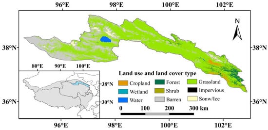
Figure 1.
Location and land use/land cover of the study area.
The QLMNP experiences a continental climate characterized by strong solar radiation, significant daily temperature fluctuations, and marked vertical variations in temperature and precipitation. Average annual temperatures range from −1.4 °C to 7.8 °C, with extremes ranging from −35.8 °C to 37.6 °C. Annual precipitation varies from 84.6 mm to 515.8 mm, while evaporation exceeds 1137.4 mm in some areas. Grassland dominated ecosystems cover 62.1% of the area, including lowland meadows, temperate steppes, and alpine desert systems [43].
2.2. Data Sources
In this study, we collected multi-source remote sensing data spanning meteorological, topographical, soil, land use, and socio-economic domains from 2000 to 2020. Table 1 summarizes the data sources. To ensure spatial consistency, all raster layers were resampled to a 1 km × 1 km grid using QGIS3.36.1. The spatial coordinate system was standardized to WGS84, and mask extraction was applied to focus on the QLMNP region. Slope values were derived from the DEM dataset, while land use/land cover (LULC) categories included cropland, forest, shrubland, grassland, water, snow/ice, barren, impervious, and wetland. We analyzed 30 m resolution data and employed a land transition matrix to identify areas converted to cropland, forest, grassland, and impervious between 2000 and 2020. The “Zonal Statistics” tool was then used to calculate transition areas within each 1 km × 1 km grid for driver analysis.

Table 1.
Data sources used for the study.
2.3. Methods
In this study, we assessed the trends in FVC and the spatial and temporal changes in ESs within the QLMNP from 2000 to 2020. We then analyzed the primary drivers of these changes and proposed ecological restoration and land management zoning strategies based on the results (Figure 2).
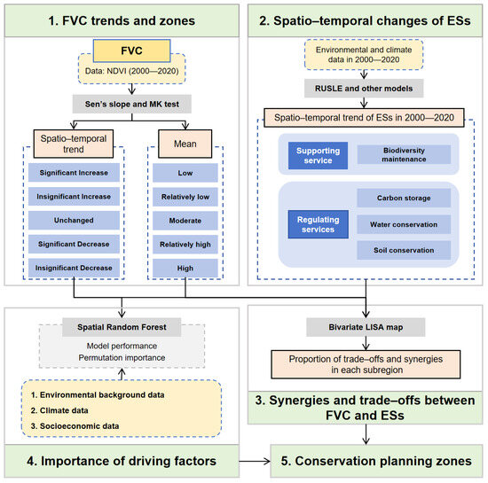
Figure 2.
Flow chart of the study.
Initially, we quantified the FVC trends using Theil–Sen median trend analysis and evaluated its statistical significance via the Mann–Kendall test. Subsequently, we classified the QLMNP into the following five zones based on the FVC trends: significantly increased (SIN), insignificantly increased (IIN), unchanged (UNC), insignificantly decreased (IDE), and significantly decreased (SDE) (Table 2). Furthermore, we categorized the study area into five vegetation zones—high (H), relatively high (RH), moderate (M), relatively low (RL), and low (L)—based on the multi-year mean FVC (Table 2).
Table 2.
Zoning classification criteria.
Next, we examined the spatial and temporal trends of the following four ESs: CS, SC, WC, and BIO. We also assessed temporal variations in ES changes across the two zoning categories. To accomplish this, we applied the global Moran’s I index to quantify the overall spatial correlation between FVC and ESs, while utilizing local bivariate Moran’s I to generate local indicators of spatial association (LISA) cluster maps. These maps visualized spatial correlations between FVC and ESs across different partitions.
Third, we identified the main drivers of increasing and decreasing FVC trends by analyzing environmental factors (including DEM, slope, pH, bulk density (BD), nitrogen (N), phosphorus (P), potassium (K), and soil organic matter (SOM)), climate variables (including precipitation (PRE), precipitation variability (PREcv), temperature (TEM), temperature variability (TEMcv), soil moisture (SM), soil moisture variability (SMcv), atmospheric CO2 concentration, and PM2.5), and anthropogenic activities. The latter encompassed land-use conversions to grassland, forest, farmland, and built-up areas, as well as GDP, population (POP), grazing pressure (GP), and nighttime light (NL). A total of 24 variables were selected for analysis. Environmental factors determine the fundamental ecological conditions in specific regions. Climate variables exert influence on vegetation growth through long-term trends and interannual fluctuations. Meanwhile, anthropogenic activities serve as direct and indirect anthropogenic drivers of ecosystem changes. We employed the SRF model to determine variable importance and generated a spatial distribution map of the most influential factors.
Finally, we integrated FVC trends, ES trade-off relationships, and spatial heterogeneity influences to delineate ecological restoration and land management zones within the QLMNP. Based on these findings, we proposed region-specific conservation and restoration measures aimed at enhancing ecosystem resilience to climate change and mitigating anthropogenic-driven ecological degradation. The detailed calculation methods are presented below.
2.3.1. Assessment of FVC
FVC is a critical indicator for evaluating the effectiveness of ecological restoration, as it reflects both the quality of ecological environments and ecosystem status [31]. In this study, we quantified FVC during 2000–2020 using NDVI with the following formula:
where NDVIveg and NDVIsoil represent the NDVI values for pure vegetation and bare soil pixels, respectively. Since FVC accounts for mixed vegetation cover, NDVIveg and NDVIsoil are dynamically determined based on the 5th and 95th cumulative frequency thresholds of the NDVI distribution [6].
2.3.2. Assessment of Ecosystem Services
In this study, we analyzed the following four ESs: WC, CS, SC, and BIO.
The WC measures an ecosystem’s capacity to intercept precipitation, regulate runoff, and purify water. It was calculated using the Water Balance Equation [5,64]:
where P, AET, and c represent the precipitation (mm), actual evapotranspiration (mm), and runoff coefficient (Table S1), respectively.
WC = P − AET − c × P
The SC quantifies an ecosystem’s ability to retain soil by reducing erosion processes. It was derived from the Revised Universal Soil Loss Equation (RUSLE) [20]:
where R, K, LS, C, and P represent the rainfall erosion factor (MJ⋅mm/hm2⋅h⋅a), soil erodibility factor (t⋅hm2⋅h/hm2⋅MJ⋅mm), slope length and slope factor (dimensionless), cover and management factor (dimensionless), and soil conservation measure factor (dimensionless), respectively.
SC = R × K × LS × (1 − C × P)
The CS is primarily driven by vegetation’s CO2 absorption capacity. Vegetation carbon sequestration was estimated using the CASA model, with a fixed organic matter-to-CO2 conversion ratio of 1:1.62 [20]:
where Gcs, Rc, and NPP represent the annual CS of vegetation (kg·ha⁻1), the carbon content in CO2 (27.27%), and the net primary productivity (NPP) (kg·ha⁻1), respectively.
Gcs = 1.62 × Rc × NPP
BIO reflects an ecosystem’s capacity to sustain genetic, species, and landscape diversity. We quantified BIO using the NPP-based method outlined in the Guidelines for Demarcating Ecological Protection Red Lines:
where Bio is the biodiversity maintenance index, NPPmean is the average NPP, Fpre is the average precipitation, Ftem is the average temperature, and Falt is the elevation factor. Data were normalized to a range of 0–1 using the min–max normalization method.
Bio = NPPmean × Fpre × Ftem × (1 − Falt)
2.3.3. Theil–Sen Median Trend Analysis and Mann–Kendall Test
We used Theil–Sen median trend analysis and Mann–Kendall test to evaluate the spatiotemporal trends and statistical significance of FVC, ESs, and their influencing factors during 2000–2020 [65], using the following equation:
where xj and xi represent the values for the jth and ith years, respectively.
The Mann–Kendall test, a non-parametric statistical method suitable for analyzing long time series data, was employed to assess the presence of significant monotonic trends. This test eliminates requirements for data linearity and normality, making it particularly appropriate for environmental datasets [65].
For a time series, where i = 1,2,…, n, the test statistic, S, is calculated as follows:
The standardized test statistic Z is calculated as follows:
where xj and xi represent the observations for the jth and ith years, respectively, and n represents the total number of observations. At a significance level of α = 0.05, the null hypothesis of no trend is rejected if ∣Z∣ > 1.96, the critical value for two-tailed testing.
2.3.4. Bivariate Spatial Correlation Analysis
The bivariate Moran’s I statistic for geographic data is used to measure the spatial correlation and heterogeneity among different variables in the same region [66]. In this study, we employed both global and local bivariate Moran’s I to examine the spatial correlation of FVC and ESs across the entire region and identify the distribution of local spatial associations [67]. The formula for the bivariate Moran’s I statistic is presented as follows [68]:
where Iel is the global bivariate Moran’s I; Iel > 0 indicates positive spatial correlation, while Iel < 0 indicates negative spatial correlation; Iel represents the local bivariate Moran’s I; n is the total number of grid cells; Wij is the spatial weight matrix; and zei and zlj represent the values of indicators e and l at locations i-th unit and j-th unit, respectively. We assessed the non-parametric significance of spatial associations at the 5% significance level using 999 random permutations [68]. The spatial relationships between FVC and ESs were categorized into the following four types: high–high (H-H), low–low (L-L), low–high (L-H), high–low (H-L), and not significant (N.S.). Spatial correlation analysis was performed using Geoda 1.12 (http://geodacenter.github.io/) (accessed on 16 July 2024).
2.3.5. Spatial Random Forest
SRF mitigates spatial autocorrelation in model residuals while providing robust variable importance assessment. We employed the “spatialRF” and “ranger” packages in R4.3.1 to construct SRF models for analyzing five FVC trend categories [69].
To account for spatial heterogeneity and capture fine-scale variations, we discretized the QLMNP region into 5 km × 5 km grid cells. The dependent variable represented the proportion of each trend category within individual grid cells, while the predictor variables comprised 24 factors previously described, including environmental variables, climatic variables, and anthropogenic influences. Specifically, the land transfer factor is expressed as the area ratio of land converted to cropland, forest, grassland, and impervious between 2000 and 2020; DEM, slope, pH, BD, N, P, K, and SOM are represented by their spatial averages across individual rasters; and the remaining 12 variables were quantified using the mean slope magnitude within each grid cell over the same period (2000–2020).
We explored spatial dependency through distance thresholds (0, 10, 100, 200, and 400 km) and interactions using the feature_engineer() function. Collinearity reduction was achieved through auto_cor() and auto_vif(), retaining only variables with VIF < 7.5 and correlation < 0.7. The SRF models were developed using rf_spatial() with 30 repetitions to account for uncertainty through rf_repeat(). The model’s performance was evaluated using out-of-bag R2 and RMSE. Variable importance was assessed via permutation importance, while response curves elucidated predictor–outcome relationships [39].
2.3.6. Zoning Method
The zoning method was developed to support the implementation of ERPs and land-use management strategies within the QLMNP. We first classified the park into distinct regions based on the temporal trends in FVC from 2000 to 2020. This classification allowed us to identify regions with similar vegetation dynamics and trends. Next, we assessed trade-offs and synergies among the four ESs in each region and superimposed the FVC trend classification with ES assessments. This allowed us to understand the interrelationships between vegetation dynamics and ESs on a regional scale. To further refine our analysis, we integrated spatial distributions of key drivers—such as environmental factors (e.g., DEM and soil properties), climatic factors (e.g., TEP and PRE), and anthropogenic activities (e.g., GP and land-use changes)—using the results from the SRF model. By overlaying these drivers onto the FVC and ES data, we created an integrated vector grid framework that aligned ecological boundaries with administrative divisions to ensure both ecological relevance and practical management feasibility. Based on this integrated analysis, we identified 12 distinct ecological zones within the QLMNP. These zones were specifically designed to address site-specific restoration needs, with areas that share similar ecological attributes and restoration requirements being aggregated into a single zone.
3. Results
3.1. FVC Trend in the QLMNP
From 2000 to 2020, the FVC in the QLMNP exhibited a consistent upward trend, with 84.31% of the study area demonstrating increased FVC. These increases were predominantly distributed in the western and eastern regions, which are dominated by grassland. Conversely, 8.82% of the study area exhibited FVC declines, with 0.66% of this region showing significant decreases (p < 0.05). These declines were concentrated primarily in the central and eastern regions, where cropland and barren constitute dominant land covers. The remaining 6.87% of the study area maintained stable FVC (Figure 3a,b), primarily corresponding to forest and barren. Significant recovery was observed across all vegetation categories, with particular emphasis on regions with low FVC (Figure 3d). The mean FVC in the QLMNP demonstrated a significant upward trend (p < 0.001) during 2000–2020, exhibiting an annual growth rate of 0.0028 (R2 = 0.55). Furthermore, trend analysis revealed that FVC in both SDE and IDE regions continued to decrease over the study period, thereby necessitating urgent conservation and restoration initiatives (Figure S1). Our analysis further revealed a negative correlation between FVC magnitude and IDE proportionality, as well as demonstrated positive associations with SIN distribution patterns. Specifically, regions with higher FVC exhibited greater IDE contributions, whereas lower FVC regions showed increased SIN shares. These findings suggest that restoration efforts are most effective in low FVC regions, while high FVC regions may be susceptible to degradation processes.
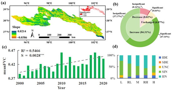
Figure 3.
Trends and proportions of FVC in the QLMNP from 2000 to 2020: (a) spatial distribution and significance of FVC trends; (b) proportional distribution of FVC trend types; (c) temporal trend of mean FVC; (d) FVC trend types across vegetation cover categories. R2: model fit; S: annual mean FVC growth rate. *** p < 0.001. L: low FVC; RL: relatively low FVC; M: moderate FVC; RH: relatively high FVC; H: high FVC; SIN: significant increase; IIN: insignificant increase; UNC: unchanged; SDE: significant decrease; IDE: insignificant decrease.
3.2. Temporal and Spatial Trends in Ecosystem Services in the QLMNP
We analyzed changes in four ESs in the QLMNP from 2000 to 2020 (Figure 4 and Figures S3–S6). The average SC was 166.56 t/hm2, with 40.99% of the study area exhibiting increases, primarily in the eastern and northern regions. Conversely, the central and western regions showed significant growth (Figure 4a). SC exhibited rapid growth between 2005 and 2010 but slowed down after 2010, maintaining an overall upward trend (Figure S3). Notably, SC significantly increased in zones with low FVC and relatively high FVC values. Specifically, the SC growth rate was 2.31 t/hm2·yr in areas with significant vegetation restoration, while the decline rate reached 2.18 t/hm2·yr in degraded zones (Figure S1). This suggests that even high FVC zones may experience SC loss if vegetation degradation occurs.
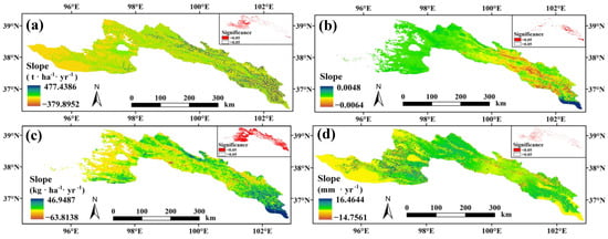
Figure 4.
Spatial distribution of the trends in four ecosystem services from 2000 to 2020: (a) spatial distribution of soil conservation trend; (b) spatial distribution of biodiversity maintenance trend; (c) spatial distribution of carbon sequestration trend; (d) spatial distribution of water conservation trend.
The average BIO in the QLMNP was 0.05, with only 2.39% of the study area showing increases, mainly in the southeastern region with significant vegetation recovery (Figure 4b). In contrast, 13.72% of the area exhibited decreases, concentrated in the central and eastern regions, including a sharp decline in 2010 (Figure S4). Over the study period, the UNC zone had the highest average BIO, but it experienced a gradual decline (0.0006 per year). This was followed by the SDE zone and IDE zone, both showing marked BIO reductions, whereas the SIN and IIN zones displayed lower average BIO with marginal increases (Figure S1). Additionally, BIO exhibited a slight downward trend in high FVC areas (Figure S1), indicating that conservation efforts in high BIO zones yielded limited success, potentially overlooking biodiversity gains in low FVC areas (Figure S1).
The mean CS value across the QLMNP was 755.34 kg/hm2, with most areas showing increases except for 2.92% (primarily in the central region) where declines occurred (Figure 4c). CS steadily increased from 2000 to 2015 but showed localized declines afterward (Figure S5). Notably, CS in degraded areas declined slowly (3.16 kg/hm2·yr), while non-degraded areas experienced significant growth (Figure S1).
The average WC in the QLMNP was 93.68 mm, with 8.91% of the study area experiencing reductions, mainly in the western and eastern regions (Figure 4d). WC remained stable in 17.73% of the area, including the western desert region and Hala Lake, which lacks significant water retention capacity, whereas stability in the eastern region suggests WC nearing capacity limits (Figure 4d). WC increased gradually between 2000 and 2010 but declined afterward (Figure S6). Furthermore, the average WC was higher in the IIN, IDE, and SDE zones, indicating an enhanced WC in these areas. While the WC in the SIN zone remained relatively low, it showed a marginal upward trend (Figure S1). Contrary to the other ESs, the WC peaked in moderate and relatively high FVC zones, with no distinct gradient between high and low FVC zones. This implies a potential trade-off among ESs in the region, where a higher FVC did not universally enhance the WC, and our hypothesis suggests complex interactions between FVC and WC (Figure S1).
3.3. Spatial Correlation Analysis of FVC and Ecosystem Services
The global spatial autocorrelation analysis revealed significant positive spatial clustering of FVC and ES trends in the QLMNP (Moran’s I > 0, p < 0.001), indicating strong spatial dependence across the study area. Notably, the strongest clustering intensity was observed for the FVC, BIO, and CS trends, whereas weaker autocorrelation existed for the SC and WC trends (Figure S7). The LISA maps demonstrated distinct spatial clustering patterns. For the CS trends, the H-H aligned with southeastern and northern forest and grassland exhibiting dense forest and vigorous vegetation growth, while the L-L occupied 26.36% of barren in the west-central region characterized by low FVC and CS (Figure S7b). In central and eastern regions with moderate and high FVC but slow recovery rates, the BIO trends exhibited dominant L-L (Figure S7c). Similarly, the SC trends showed L-L in western barren, contrasting with dispersed H-H in the southeastern region indicative of accelerated SC increase (Figure S7d). Notably, despite initially low WC, H-H emerged in central and southeastern regions where vegetation restoration drove WC enhancement (Figure S7e).
Across vegetation zones, the FVC trends exhibited enhanced H-H in the relatively high and moderate FVC zones, whereas L-L dominated in the high FVC region (Figure S8). This spatial pattern reflects more rapid and effective vegetation recovery in the relatively low and moderate FVC zones, potentially attributed to their ecological restoration interventions, while the high FVC zone displayed slower growth rates despite already high vegetative cover (Figure S8). The CS trends demonstrated inverse relationships with the FVC gradients. The H-H proportions decreased, while the L-L increased as the FVC rose. Notably, the CS growth rates remained elevated even when the FVC increased slowed, likely because of the high FVC region’s dominance by forest ecosystems (Figure S8). The BIO trend distributions closely mirrored those of the FVC, with the L-L prevalence peaking in the high FVC region. This suggests that the BIO gains remained constrained despite restoration efforts in the high FVC region (Figure S8). The SC trends exhibited near-exclusive L-L in the low FVC region, where the SC and WC capacities remain critically limited despite the partial restoration (Figure S8). Conversely, the H-H patterns in the CS trends aligned with those of the FVC, indicating sufficient FVC to mitigate the soil erosion even during periods of stagnant the FVC growth (Figure S8). The WC trend distributions exhibited negative correlations with the FVC gradients. The L-L proportions declined with an increasing FVC, whereas the H-H became more spatially uniform. Additionally, the L-L shares of the SC and WC were higher in the IIN and SIN zones compared to the IDE and SDE zones, underscoring persistent vulnerabilities in the SC and WC despite restoration efforts in low FVC regions (Figure S8).
The bivariate spatial correlation analysis revealed significant positive associations between the FVC trends and most ESs (BIO, CS, and WC). However, negative correlations emerged between the SC-FVC, BIO-WC, and BIO-SC pairs (Figure 5). These patterns suggest that vegetation restoration intensities generally promote the WC, BIO, and CS improvements but suppress SC accumulation.
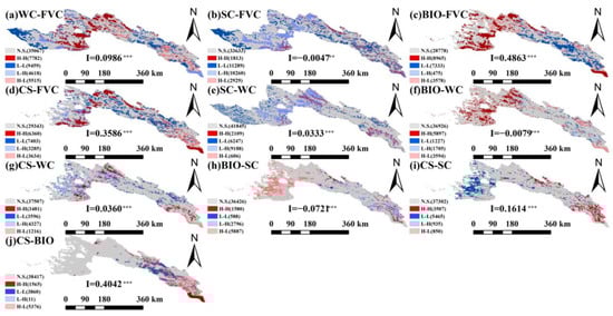
Figure 5.
Bivariate LISA maps of pairwise ecosystem service indicator trends. H-H: high–high clustering; L-L: low–low clustering; L-H: low–high clustering; H-L: high–low clustering; N.S.: not significant. **: p < 0.01; ***: p < 0.001.
Synergistic clustering (H-H, L-L) dominated the FVC-WC, FVC-BIO, and FVC-CS relationships in the central-southeastern regions, where vegetation recovery drove synchronous ES enhancements (Figure 5a,c,d). However, the trade-offs (H-L, L-H) emerged between the SC-FVC in the degraded zones and the WC-FVC in the overgrown vegetated areas (Figure 5a,b and Figure S8). In central regions, the high WC trends coexisted with the BIO/CS gains but the SC declines, primarily in moderate and relatively low zones, suggesting that the WC improvements did not directly stimulate SC recovery (Figure 5e–g and Figure S8). The BIO-SC trade-offs were most pronounced. The BIO gains in central regions with declining SC trends stemmed from ecological restoration efforts, whereas BIO losses in southern high-SC zones resulted from vegetation degradation (Figure 5h and Figure S8). The CS-SC exhibited L-L in west-central barren and H-H in the southeastern forest, reflecting soil erosion risks in the low FVC region and stable CS in the high FVC region (Figure 5i). The CS-BIO exhibited mixed clustering patterns, including L-L and H-L. The L-L in the east-central grassland likely resulted from degradation, while the H-Ls were primarily driven by agricultural conversion and artificial grassland development, suggesting land-use intensification as a key mechanism (Figure 5j and Figure S8).
3.4. Analysis of the Driving Factors of Vegetation Trends in the QLMNP
The SRF model revealed significant spatial heterogeneity in the relative importance of driving factors. We applied SRF to quantify relationships between multiple environmental variables and FVC trends. The results demonstrate strong explanatory power (R2 > 60% for SIN/IIN, R2 > 50% for UNC/IDE, and R2 > 40% for SDE), partially explaining the influences of various factors on FVC trends (Table S2).
Variable importance analysis and response curve evaluations revealed distinct regulatory roles of the factors. Among the four trends, PREcv emerged as the most critical factor, except for UNC (Figure 6). When PREcv < 20%, increasing PREcv reduced SDE, IDE, and IIN shares while increasing SIN dominance (Figure S9a,d,e). However, UNC remained relatively stable (Figure S9c). When PREcv > 20%, only the UNC increased sharply, while the other trends stabilized (Figure S9c). Conversely, higher PREcv values gradually diminished the SIN and UNC shares but enhanced the remaining categories (Figure S9a,c). These patterns suggest the optimal PREcv thresholds for vegetation recovery, where a moderate PREcv promotes recovery, while extreme PREcv values may become detrimental (Figure S9a,c). The SMcv also exhibited threshold effects. When SMcv ranged between 0 and 10%, an increase in SMcv boosted SIN and UNC shares while suppressing others (Figure S9a,c). However, when SMcv > 10%, limited impact on the trend distributions was observed. Notably, the TEMcv emerged as the primary determinant of UNC dynamics. The elevated TEMcv reduced UNC shares and triggered vegetation degradation once temperature trends exceeded 0.01 °C/yr (Figure S9c).
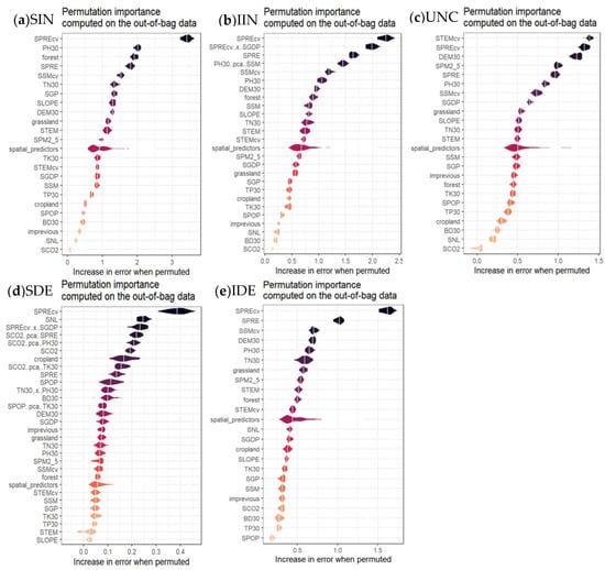
Figure 6.
Permutation importance computed on the out-of-bag data of the five change trends. The “S” before the indicator abbreviation represents annual change rate during 2000–2020. SIN: significant increase, IIN: insignificant increase; UNC: unchanged; SDE: significant decrease; IDE: insignificant decrease.
Changes in the NL constituted a critical factor influencing SDE patterns (Figure 6d). A higher NL correlated with increased SDE proportions, suggesting NL exerted inverse effects on vegetation recovery (Figure S9d). Conversely, a reduced GP enhanced SIN dominance, indicating that controlled grazing positively impacted vegetation restoration (Figure S9a). Additionally, expansion of forest and grassland accelerated vegetation recovery and stabilization, whereas cropland expansion promoted significant degradation (Figure S9d). These findings underscored the pivotal role of anthropogenic activities in shaping vegetation trajectories. Environmental background also has an important effect on vegetation recovery. A soil pH between 8 and 8.5 favored SIN dominance (Figure S9a). Meanwhile, steep slopes and high elevations inhibited vegetation recovery and increased degradation risks (Figure S9a,b,e). Furthermore, interactive effects among variables significantly modulate restoration outcomes. For instance, rapid GDP growth combined with high PREcv reduced IIN proportions and elevates SDE shares, whereas lower GDP growth paired with moderate PREcv promoted IIN increases (Figure S9b,d). CO2 fertilization synergized with PRE and soil properties (e.g., pH and K) to mitigate SDE prevalence (Figure S9d).
To identify grid-specific dominant factors and inform restoration strategies, we analyzed most impactful factors in the QLMNP (Figure 7). The results showed that climate-driven regions covered 34,714.08 km2, primarily in the western and central parts of the QLMNP, where PREcv exerted the strongest influence. Environmental-driven regions spanned 17,429.90 km2, with DEM dominating Hala Basin and pH influencing the eastern QLMNP. Anthropogenic-driven zones occupied 6092.64 km2 in the central and southeastern QLMNP, where GP was the primary driver (Figure 7). These results highlighted the necessity for regionally tailored restoration approaches that account for climatic, environmental, and anthropogenic gradients in the QLMNP.
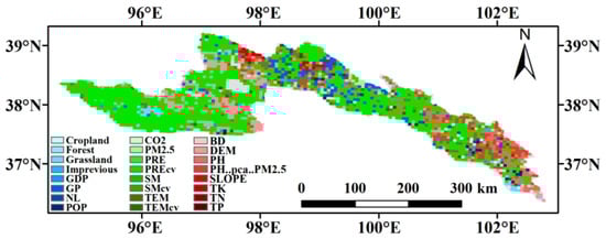
Figure 7.
Spatial distribution of dominant drivers for vegetation dynamics in the QLMNP. The blue category represents human activity factors, the green category represents climate change factors, and the red category represents environmental background factors.
3.5. Ecological Restoration Project Implementation and Land-Use Management Zones in the QLMNP
This study proposed a zoning framework for ecological protection and restoration in the QLMNP based on FVC patterns, ES relationships, driver distributions, and natural and administrative boundaries. The region was divided into 12 distinct zones, each requiring tailored conservation measures (Figure 8). This zoning approach aims to address ES optimization, and sustainable land-use practices while mitigating climate change impacts and human-induced disturbances.
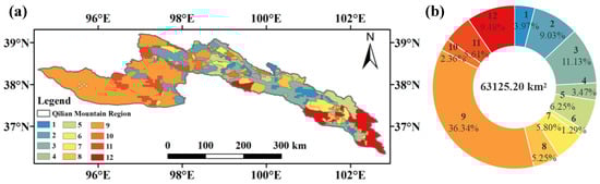
Figure 8.
Ecological zoning framework for conservation and management in the QLMNP: (a) spatial distribution of the regulatory zoning; (b) area proportion of each zone type.
Zone 1, covering 3.97% of the QLMNP’s total area and located in the central region, is characterized by a high FVC and PRE exceeding 400 mm, yet exhibits evidence of vegetation degradation. Dominated by environmental factors, ESs here show predominantly synergistic changes. To address these challenges, restoration efforts should prioritize soil condition assessments, topographic evaluations, and strategic vegetation selection, alongside enhanced monitoring and adaptive management of ecosystem processes.
Zone 2, spanning 9.03% of the QLMNP in the central-western region, receives less than 400 mm of annual PRE with high variability, exhibiting mild vegetation degradation, declines in SC, and reductions in BIO. Characterized by steep slopes and high elevations, this zone is strongly influenced by climatic and environmental factors. Recommended actions include implementing SC and WC measures, establishing windbreak systems, and planting drought-resistant shrubs and grasses to stabilize vegetation and enhance BIO.
Zone 3, occupying 11.13% of the QLMNP centrally, features a high FVC but a declining trend, with ES reductions despite adequate PRE (>400 mm). Climate factors are primary drivers of this decline. Restoration should focus on selecting resilient vegetation, optimizing water resource use, and enhancing the functionality of ESs to improve long-term stability.
Zone 4, spread across central-southeastern areas and constituting 3.74% of the QLMNP, maintains high FVC but shows mild degradation and reduced ESs. With a PRE exceeding 400 mm, human activities dominate local dynamics. Management strategies should regulate grazing and agricultural practices, implement fencing and ecological migrants, and restore native vegetation to balance land use and conservation.
Zone 5, located on the northeastern edge of the QLMNP, exhibits a trade-off between the FVC and BIO, influenced by both climatic and environmental factors. To enhance ecosystem stability and diversity, restoration efforts must prioritize FVC improvement through diverse/native vegetation planting while addressing resource heterogeneity.
Zone 6, comprising 814.00 km2 in the southeastern region, has a PRE exceeding 400 mm but shows FVC decline and WC reduction, driven primarily by environmental factors. Actions should focus on selecting appropriate vegetation, optimizing planting ratios, and implementing measures to ensure sustainable water supply for ecosystem health.
Zone 7, occupying 5.80% of the QLMNP in the central-southeastern region, demonstrates increasing FVC but declining SC, influenced by climate change and human activities. Priority measures include protecting natural forests, promoting reforestation, and stabilizing sand dunes through structural interventions.
Zone 8, covering 3316.19 km2 in the central QLMNP with a high PRE (>400 mm) and low variability, maintains healthy vegetation and synergistic ESs. Existing conservation measures should be sustained, with no immediate restoration needs identified.
Zone 9, constituting 36.34% of the QLMNP in the western region, experienced a PRE < 400 mm with high variability, resulting in the low FVC but increasing trends alongside the WC-FVC trade-offs. Effective water resource management is critical, particularly in arid zones, to ensure sustainable water availability.
Zone 10, located in the northern-central QLMNP and spanning 1490.59 km2, features a PRE > 400 mm and high FVC but faces BIO-FVC trade-offs influenced by significant human activities. Recommendations include transitioning from monoculture to polyculture systems and enhancing vegetation diversity to improve resilience.
Zone 11, comprising 5.61% of the QLMNP in the western region with PRE < 400 mm, is recovering gradually but exhibits WC-FVC trade-offs and strong environmental influences. Because of the high altitude, restoration efforts should prioritize planting water-retaining vegetation adapted to arid/high-altitude conditions to improve SC and WC.
Zone 12, situated in the southeastern QLMNP, demonstrates high and increasing FVC but experiences WC decline, driven by a low altitude and a PRE > 400 mm. Management strategies should optimize land-use planning, enhance WC infrastructure, and balance FVC with hydrological sustainability to support ecosystem health.
In summary, each zone within the QLMNP requires distinct ecological restoration strategies tailored to its specific environmental and climatic conditions, with a focus on enhancing ecosystem service provision and promoting sustainable land-use practices.
4. Discussions
The ecological restoration efforts in the QLMNP had produced significant outcomes, including enhanced FVC and improved ESs. This study systematically analyzed shifts in the FVC trends and ES enhancements associated with restoration measures implementation. Furthermore, it identified key drivers of vegetation recovery, validated the effectiveness of restoration strategies in the QLMNP, and conducted comprehensive investigations into diverse FVC trends. The results demonstrated that the FVC had substantially increased across most areas of the QLMNP, with the BIO effectively maintained, WC enhanced, soil erosion rates reduced, and CS potential augmented. Notably, the primary objectives of ecological restoration in this region had been largely achieved. However, regional disparities in restoration outcomes emphasized the necessity for adaptive management approaches [40].
4.1. Effects of Ecological Restoration Implementation
The FVC and ESs in the QLMNP exhibited an overall increasing trend over the past two decades, with only localized regions experiencing significant declines. These patterns may be attributable to the spatial limitations of hydrothermal conditions [70]. The results demonstrate that while the ecological environment in the QLMNP has achieved measurable improvements, regional disparities remain evident, highlighting the necessity for targeted protection and restoration initiatives in areas with decreasing FVC and ESs. From 2000 to 2020, FVC in the QLMNP showed a gradual eastward increase (Figure S2), likely driven by the west-to-east precipitation gradient exceeding 400 mm/yr. This spatial distribution suggests that grassland/shrub plantations are climatically suitable for regions with annual precipitation below this threshold [68].
Vegetation type and structural complexity exert critical regulation on biogeochemical cycling and energy fluxes within ecosystems, thereby contributing to the spatial heterogeneity of ecosystem services [71]. Through transpiration, vegetation modulates the water cycle, mitigates rainfall-induced erosion via root systems, and enhances CS through photosynthesis [20]. According to the water balance principle, precipitation, evapotranspiration, and runoff are the primary determinants of spatial water retention capacity patterns [20]. Within the QLMNP, increased precipitation since 2000 has enhanced FVC, resulting in reduced runoff and improved WC [72], thereby establishing a positive correlation between WC and FVC. Conversely, vegetation expansion-induced evapotranspiration has intensified water consumption, leading to lower WC in densely vegetated zones [73]. Moreover, WC exhibits higher values in high-elevation areas compared to low-elevation regions, primarily due to enhanced orographic precipitation and reduced evapotranspiration rates [74]. These zones, dominated by forests/grasslands, typically exhibit lower runoff potential and higher water retention capacities relative to cropland areas [75].
In contrast, the spatial distributions of BIO, CS, and FVC exhibited strong spatial coincidence. Areas with elevated BIO and CS were predominantly concentrated in eastern forested and vegetated grassland regions, which function as carbon sinks and habitat preserves [76]. Notably, CS primarily correlates with NPP magnitude, whereas BIO is influenced by interactions among NPP, climate variables, and topography. This distinction arises because forest exhibit greater NPP than grassland, coupled with higher precipitation and temperature in the eastern QLMNP [77]. Consequently, the maximum CS and BIO values occurred in low-elevation eastern forest, followed by grassland and cropland, with barren exhibiting minimal values. Implementation of ERPs temporarily enhances FVC and biomass, thereby promoting CS and BIO accrual through synergistic FVC-CS/BIO-FVC relationships.
According to the RUSLE equation, apart from precipitation-driven erosion, soil properties, topography, and vegetation cover constitute primary regulators of soil conservation (SC) changes. Increased FVC improves erosion control capacity, substantially reducing soil erosion rates [78]. However, vegetation restoration exhibits a threshold effect on SC enhancement [79]. Only when FVC increases exceed critical thresholds does vegetation growth sufficiently reduce soil erodibility and mitigate sediment yield [80]. Bivariate spatial correlation analyses revealed that rapid vegetation recovery in the central/western QLMNP drove significant BIO and WC improvements, indicating the efficacy of ecological policies in enhancing BIO and WC. In contrast, SC-FVC exhibited trade-offs in these regions, arising from insufficient erosion control despite enhanced WC through runoff reduction. Moreover, excessive precipitation intensities induced runoff escalation, counteracting SC benefits and creating L-H trade-offs between SC-FVC and SC-BIO. Arid zone precipitation increases also stimulated evapotranspiration, lowering temperatures and inhibiting photosynthesis, ultimately reducing CS and causing CS-WC aggregation in midwestern regions.
Current restoration plans emphasize sustainability, but vegetation expansion risks creating trade-offs with SC and WC. Therefore, future studies must establish vegetation growth thresholds to balance ES improvements [81]. Strategic adjustments are required for project implementation; in regions with successful vegetation recovery, prioritizing protection and monitoring over continued area expansion proves essential [79].
4.2. Influences of Ecological Effectiveness
The prevailing scholarly consensus on ecological restoration recognizes climate change, environmental context, and anthropogenic activities as primary drivers of ecosystem dynamics [7,35,82]. However, the relative importance of these factors exhibits spatial variability, with scale-dependent discrepancies observed in their influence on ecological processes [74]. Specifically, factors dominating ecosystem change at one scale may lose significance at larger or smaller scales.
This study reveals that climate change exerts the most pronounced impact (60% of the QLMNP), primarily driven by the region’s extreme PREcv [41]. This pattern underscores precipitation’s critical role in modulating vegetation stress responses across the QLMNP. Notably, the western and central QLMNP exhibit heightened susceptibility to precipitation fluctuations, attributable to spatial–temporal precipitation imbalances that amplify vegetation moisture sensitivity. The QLMNP’s arid/semi-arid ecology demonstrates a nonlinear response to precipitation increases. While elevated precipitation during growing seasons can enhance vegetative productivity [83], excess rainfall may induce subsurface oxygen deficiency, microbial proliferation, and nutrient leaching losses [84]. Conversely, temperature assumes paramount control over stable vegetation zones, where threshold-based moisture evaporation dynamics disrupt photosynthetic processes. When ambient temperatures exceed critical thresholds, soil moisture depletion accelerates, inducing stomatal closure to conserve water—a physiological trade-off that reduces net carbon assimilation and stifles vegetative growth [85]. This negative feedback mechanism can mitigate precipitation-driven benefits, creating climatic–vegetation interaction complexities.
Contrary to previous empirical findings, our results did not reveal a positive effect of elevated CO2 concentrations on vegetation recovery in the QLMNP [85]. This divergence might be explained by the region’s predominantly grassland-dominated ecosystems, which lack the rapid CO2 fertilization response characteristic of forested systems. Furthermore, the slow temporal trajectory of CO2 enrichment implies limited detection capacity in short-term studies, which fails to capture the long-term effects of CO2 fertilization mechanisms [82]. The elevated CO2 levels in the QLMNP’s cold, high-altitude climate intensify nitrogen limitation, thereby restricting plant productivity through biochemical constraints [86]. Notwithstanding these complexities, our analysis highlights a detrimental interaction between CO2 and precipitation, which exacerbates vegetation degradation (Figure 6d). This phenomenon may be attributed to the observation that an increase in CO2 concentration can enhance water use efficiency in arid regions, thereby promoting vegetation productivity [86] and curtailing the degradation trend of vegetation.
Beyond climatic variables, environmental conditions and anthropogenic activities significantly modulate vegetation dynamics. Environmental conditions encompasses physiographic parameters (e.g., elevation gradients) and edaphic properties, which structure local hydrothermal regimes and regulate soil nutrient cycles [87,88]. Topography exerts microscale dominance over plant growth in arid landscapes [89]. A notable example is the Hala Lake region, where topographical features such as elevation have been observed to exert a pronounced influence. This is likely attributable to the fact that these areas receive less precipitation, leading to a situation where vegetation may be more dependent on microclimatic effects associated with elevation.
Anthropogenic drivers manifest acute short-term impacts through land-use conversions [82]. Specifically, grassland reclamation programs have altered land cover patterns and enhanced restoration efficacy [6]. Cropland expansion accelerates soil degradation through erosion processes. Urbanization-induced NL [9] disrupts ecosystem functioning. Socio-economic factors exhibit limited explanatory power in the QLMNP’s ecological dynamics, with GP emerging as a critical anthropogenic stressor. The central-southeastern regions of the QLMNP experience heightened anthropogenic disturbance, driven by intensive agro-pastoral activities [26]. Policy interventions, such as subsidized grazing cessation programs and ecological compensation mechanisms, have successfully reduced herbivory impacts while enhancing FVC and CS [90]. These outcomes underscore that land-use management strategies constitute more significant determinants of restoration success than climatic variables in this region.
Climate factors exhibit strong interactions with social variables, suggesting that ecological restoration policies must prioritize climate change adaptation [82]. Simultaneously, the development of climate-resilient livelihoods (such as ecotourism) should be strategically integrated to enhance community economic resilience and institutional capacity.
While ERPs are vital for environmental improvement, they face multifaceted challenges. Empirical evidence indicates that drought-induced NDVI declines can negate restoration benefits [10]. Vegetation expansion has also been associated with reduced surface runoff, creating downstream groundwater depletion risks that compromise vegetation health [24]. Strategic interventions including drought-resistant species cultivation and sustainable water cycle management are urgently needed [91].
Ecological restoration initiatives funded through policy subsidies aim to reduce agricultural and pastoral activities in target regions, with the intended outcome of restoring ecosystems. However, during the post-project phase, farmers and herders may revert to land-use intensification practices (such as expanding cropland or increasing grazing pressures) due to insufficient alternative livelihoods, thereby jeopardizing long-term ecological gains [82]. To mitigate this risk, it is imperative to implement technical training programs and foster sustainable livelihood options through the development of alternative industries [92]. Addressing these systemic challenges is critically important for enhancing the overall efficacy of ecological restoration and ensuring the long-term sustainability of ecosystem governance.
4.3. Implications for Zoning Management
This study has developed zoning-based conservation and management strategies for the 12 delineated ecological zones in the QLMNP, emphasizing FVC improvement, ES optimization, sustainable land-use planning, and climate-human activity impact mitigation. The framework highlights that 46.55% of the QLMNP falls under ecological protection zones, indicating persistent ecological vulnerability and environmental stress, particularly in western and northern regions characterized by low FVC and ESs. These areas require long-term investment in restoration efforts, necessitating strict protection protocols, including minimizing anthropogenic disturbances, enhancing vegetation rehabilitation initiatives, and implementing financial mechanisms through ecological compensation [93].
For regions with relatively stable ecosystems, future warming-humidification trends may favor vegetation recovery [94], suggesting management strategies should prioritize ecological equilibrium preservation, sustainable ecotourism development, and green industry promotion to advance climate-resilient economic growth while strictly regulating land-use changes to avoid ecosystem integrity compromise. Regional studies reveal context-dependent synergies and trade-offs in ecosystem services. FVC-WC trade-offs dominate certain areas, whereas BIO and restoration synergies characterize others. Differential management approaches are thus essential, guided by regional ecological function typology. In zones with pronounced service trade-offs, land-use policies should enhance system stability and adaptive capacity through optimal spatial planning (e.g., prioritizing high-functionality areas for conservation) [27].
The study underscores water resources’ pivotal role in maintaining ecosystem resilience, as hydrological regulation capacity in QLMNP has declined because of watershed contraction [26]. Future management must prioritize water resource protection, including accelerating hydroecological research investments, strengthening long-term hydrological monitoring networks, optimizing water allocation strategies, and developing GIS-remote sensing integrated hydrological prediction models to adapt to climate change scenarios [95]. Policy-wise, QLMNP’s sustainable development requires multidimensional governance through legal frameworks, financial mechanisms (e.g., ecological compensation), and community engagement to foster participatory governance [96]. Precision-aligned ecological compensation policies are critical for high-conservation-value areas, while collaborative initiatives with local communities should strengthen livelihood diversification programs to ensure sustainable income generation without compromising ecological integrity.
4.4. Limitations
This study analyzed spatial–temporal patterns of vegetation dynamics and ESs using remotely sensed data, identified drivers of vegetation trends, but acknowledges several limitations. First, although the 21-year dataset provides substantial temporal coverage, it remains insufficient for assessing century-scale ecosystem evolution, suggesting a need for multi-decadal datasets in future analyses [41]. Second, the ES assessment framework excluded critical functions such as food production and tourism services, limiting its comprehensiveness. Expansion to additional ES categories would enhance holistic ecosystem evaluation. Third, this study neglects other socio-economic influences such as policy interventions and community engagement, which may exert non-linear effects on ecosystems. Incorporating these socio-economic variables in future models could elucidate feedback mechanisms between human activities and ES provision. And also, the temporal lag effect of climate factors was not accounted for, potentially underestimating ecosystem responses to climatic shifts. Integrating time-lag analysis into predictive models would improve assessment accuracy. Finally, ESs exhibit spatial fluidity rather than static distributions, rendering rigid zoning frameworks less effective. Future studies could adopt machine learning algorithms to develop adaptive zoning protocols that account for functional spatial heterogeneity and dynamic environmental changes. Despite these limitations, this research provides foundational insights for ecological planning in QLMNP. Future improvements should focus on enhancing data resolution, integrating multi-scale drivers, and refining modeling methodologies to achieve higher precision in ES assessments.
5. Conclusions
This study conducted a comprehensive analysis of ecological restoration outcomes in the QLMNP between 2000 and 2020. We mapped vegetation trend zones, quantified spatial–temporal variations in FVC and ESs, examined trade-offs and synergies among FVC and ESs, and identified key drivers of restoration success using SRF. The results revealed 84.31% of QLMNP exhibited vegetation recovery/stabilization trends, while 8.82% showed degradation, primarily concentrated in high FVC regions. Most ESs demonstrated positive trends across QLMNP. 0.72% of areas exhibited SC decline, 13.72% showed BIO reduction, 2.92% had CS decline, and 8.91% experienced WC decrease. Spatial autocorrelation analysis revealed significant positive clustering, as follows: H-H correlations between FVC and WC in the west, and L-L associations for CS-SC and FVC-BIO in the east. Bivariate spatial regression highlighted complex trade-offs: SC-FVC/WC-FVC/BIO-WC/BIO-SC in the west, and WC-FVC/CS-FVC/BIO-WC/CS-BIO in the east, underscoring restoration process intricacies. Notably, PREcv emerged as the dominant driver of vegetation trends across 85.49% of QLMNP, except stabilization zones. Degradation correlated with increasing NL, while recovery aligned with decreasing GP. Land-use change exhibited abrupt effects on restoration outcomes. Beyond climatic and anthropogenic factors, environmental background variables exerted strong modulatory influences, interacting with other drivers in non-linear ways.
Our analysis demonstrates the heterogeneous spatiotemporal dynamics of the QLMNP’s ecological restoration, revealing complex driver hierarchies. Based on these findings, we propose zoning-based management strategies for the QLMNP that adapt conservation and restoration measures to region-specific biophysical, climatic, and socio-economic contexts, offering practical guidance for large-scale ecological projects in the QLM.
Supplementary Materials
The following supporting information can be downloaded at: https://www.mdpi.com/article/10.3390/rs17081402/s1, Table S1: P-Factor and Runoff Coefficient for Each Land Cover/Land Use Type; Table S2: Model Performance for Each Trend; Figure S1: Temporal Trends of FVC and Four Ecosystem Services in Increase-Decrease Categories and High-Low Categories from 2000 to 2020; Figure S2: Spatial Distribution of FVC from 2000 to 2020; Figure S3: Spatial Distribution of Soil Conservation from 2000 to 2020; Figure S4: Spatial Distribution of Biodiversity Maintenance from 2000 to 2020; Figure S5: Spatial Distribution of Carbon Sequestration from 2000 to 2020; Figure S6: Spatial Distribution of Water Conservation from 2000 to 2020; Figure S7: Spatial autocorrelation tests of trends for FVC and four ecosystem services. H-H represents High-High clustering, L-L represents Low-Low clustering, L-H represents Low-High clustering, H-L represents High-Low clustering, and N.S. indicates Not Significant. I denotes the global spatial autocorrelation coefficient, with * indicating p < 0.05, ** indicating p < 0.01, and *** indicating p < 0.001; Figure S8: Proportional of Different Clustering Patterns for Spatial Autocorrelation and Bivariate Spatial Correlation in QLMNP; Figure S9: Response curves of the area proportions for each trend with different influencing factors.
Author Contributions
Conceptualization, X.Y. and F.L.; methodology, X.Y., Z.Z. and F.L.; formal analysis, X.Y. and Z.Z.; writing—original draft preparation, X.Y.; writing—review and editing, X.Y., F.L., Z.Z., H.Z., H.L. and Z.S.; visualization, X.Y.; supervision, F.L., H.Y., B.Z. and X.W.; funding acquisition, H.Z. All authors have read and agreed to the published version of the manuscript.
Funding
This study was funded by the National Natural Science Foundation of China (32371684), National Natural Science Foundation of China Joint Fund Project (U21A20186), and Evaluation Project on the Ecological Protection and Construction Achievements of Qilian Mountain National Park (Qinghai Area) and Qilian Mountain Region (Qinglinbao [2024] No. 461).
Data Availability Statement
The original contributions presented in this study are included in the article/Supplementary Material. Further inquiries can be directed to the corresponding author.
Conflicts of Interest
The authors declare no conflicts of interest.
References
- Wang, C.; Zhao, H. The Assessment of Urban Ecological Environment in Watershed Scale. Procedia Environ. Sci. 2016, 36, 169–175. [Google Scholar] [CrossRef]
- Balkanlou, K.R.; Müller, B.; Cord, A.F.; Panahi, F.; Malekian, A.; Jafari, M.; Egli, L. Spatiotemporal dynamics of ecosystem services provision in a degraded ecosystem: A systematic assessment in the Lake Urmia basin, Iran. Sci. Total Environ. 2020, 716, 137100. [Google Scholar] [CrossRef] [PubMed]
- Cao, Y.; Kong, L.; Zhang, L.; Ouyang, Z. Spatial characteristics of ecological degradation and restoration in China from 2000 to 2015 using remote sensing. Restor. Ecol. 2020, 28, 1419–1430. [Google Scholar] [CrossRef]
- Huang, L.; Cao, W.; Xu, X.; Fan, J.; Wang, J. Linking the benefits of ecosystem services to sustainable spatial planning of ecological conservation strategies. J. Environ. Manag. 2018, 222, 385–395. [Google Scholar] [CrossRef]
- Shao, Q.; Liu, S.; Ning, J.; Liu, G.; Yang, F.; Zhang, X.; Niu, L.; Huang, H.; Fan, J.; Liu, J. Assessment of ecological benefits of key national ecological projects in China in 2000–2019 using remote sensing. Acta Geogr. Sin. 2022, 77, 2133–2153. [Google Scholar] [CrossRef]
- Niu, L.; Shao, Q.; Ning, J.; Liu, S.; Zhang, X.; Zhang, T. The assessment of ecological restoration effects on Beijing-Tianjin Sandstorm Source Control Project area during 2000–2019. Ecol. Eng. 2023, 186, 106831. [Google Scholar] [CrossRef]
- Ma, S.; Wang, L.J.; Wang, H.Y.; Jiang, J.; Zhang, J. Multiple ecological effects and their drivers of ecological restoration programmes in the Qinghai-Tibet Plateau, China. Land Degrad. Dev. 2023, 34, 1415–1429. [Google Scholar] [CrossRef]
- Xu, X.; Zhang, D.; Zhang, Y.; Yao, S.; Zhang, J. Evaluating the vegetation restoration potential achievement of ecological projects: A case study of Yan’an, China. Land Use Policy 2020, 90, 104293. [Google Scholar] [CrossRef]
- Wang, Z.; Fu, B.; Wu, X.; Wang, S.; Li, Y.; Feng, Y.; Zhang, L.; Hu, Y.; Cheng, L.; Li, B. Distinguishing Trajectories and Drivers of Vegetated Ecosystems in China’s Loess Plateau. Earth’s Future 2024, 12, e2023EF003769. [Google Scholar] [CrossRef]
- Li, M.; Yu, H.; Meng, B.; Sun, Y.; Zhang, J.; Zhang, H.; Wu, J.; Yi, S. Drought reduces the effectiveness of ecological projects: Perspectives from the inter-annual variability of vegetation index. Ecol. Indic. 2021, 130, 108158. [Google Scholar] [CrossRef]
- LaPaix, R.; Freedman, B.; Patriquin, D. Ground vegetation as an indicator of ecological integrity. Environ. Rev. 2009, 17, 249–265. [Google Scholar] [CrossRef]
- Foody, G.M. Editorial: Ecological applications of remote sensing and GIS. Ecol. Inform. 2007, 2, 71–72. [Google Scholar] [CrossRef]
- Li, Y.; Cao, Z.; Long, H.; Liu, Y.; Li, W. Dynamic analysis of ecological environment combined with land cover and NDVI changes and implications for sustainable urban–rural development: The case of Mu Us Sandy Land, China. J. Clean. Prod. 2017, 142, 697–715. [Google Scholar] [CrossRef]
- Yang, C.; Zhang, C.; Li, Q.; Liu, H.; Gao, W.; Shi, T.; Liu, X.; Wu, G. Rapid urbanization and policy variation greatly drive ecological quality evolution in Guangdong-Hong Kong-Macau Greater Bay Area of China: A remote sensing perspective. Ecol. Indic. 2020, 115, 106373. [Google Scholar] [CrossRef]
- Costanza, R.; d’Arge, R.; de Groot, R.; Farber, S.; Grasso, M.; Hannon, B.; Limburg, K.; Naeem, S.; O’Neill, R.V.; Paruelo, J.; et al. The value of the world’s ecosystem services and natural capital. Nature 1997, 387, 253–260. [Google Scholar] [CrossRef]
- Díaz, S.; Pascual, U.; Stenseke, M.; Martín-López, B.; Watson, R.T.; Molnár, Z.; Hill, R.; Chan, K.M.A.; Baste, I.A.; Brauman, K.A.; et al. Assessing nature’s contributions to people. Science 2018, 359, 270–272. [Google Scholar] [CrossRef]
- Zhang, D.; Jia, Q.; Xu, X.; Yao, S.; Chen, H.; Hou, X.; Zhang, J.; Jin, G. Assessing the coordination of ecological and agricultural goals during ecological restoration efforts: A case study of Wuqi County, Northwest China. Land Use Policy 2019, 82, 550–562. [Google Scholar] [CrossRef]
- Dymond, J.R.; Ausseil, A.-G.E.; Ekanayake, J.C.; Kirschbaum, M.U.F. Tradeoffs between soil, water, and carbon—A national scale analysis from New Zealand. J. Environ. Manag. 2012, 95, 124–131. [Google Scholar] [CrossRef]
- Tomscha, S.A.; Gergel, S.E. Ecosystem service trade-offs and synergies misunderstood without landscape history. Ecol. Soc. 2016, 21, 43. [Google Scholar] [CrossRef]
- Li, G.; Jiang, C.; Gao, Y.; Du, J. Natural driving mechanism and trade-off and synergy analysis of the spatiotemporal dynamics of multiple typical ecosystem services in Northeast Qinghai-Tibet Plateau. J. Clean. Prod. 2022, 374, 134075. [Google Scholar] [CrossRef]
- Wang, L.-J.; Ma, S.; Qiao, Y.-P.; Zhang, J.-C. Simulating the Impact of Future Climate Change and Ecological Restoration on Trade-Offs and Synergies of Ecosystem Services in Two Ecological Shelters and Three Belts in China. Int. J. Environ. Res. Public Health 2020, 17, 7849. [Google Scholar] [CrossRef]
- Ma, S.; Wang, L.-J.; Jiang, J.; Chu, L.; Zhang, J.-C. Threshold effect of ecosystem services in response to climate change and vegetation coverage change in the Qinghai-Tibet Plateau ecological shelter. J. Clean. Prod. 2021, 318, 128592. [Google Scholar] [CrossRef]
- Liu, Y.; Liu, S.; Sun, Y.; Sun, J.; Wang, F.; Li, M. Effect of grazing exclusion on ecosystem services dynamics, trade-offs and synergies in Northern Tibet. Ecol. Eng. 2022, 179, 106638. [Google Scholar] [CrossRef]
- Li, R.N.; Zheng, H.; O’Connor, P.; Xu, H.S.; Li, Y.K.; Lu, F.; Robinson, B.E.; Ouyang, Z.Y.; Hai, Y.; Daily, G.C. Time and space catch up with restoration programs that ignore ecosystem service trade-offs. Sci. Adv. 2021, 7, eabf8650. [Google Scholar] [CrossRef] [PubMed]
- Sun, J.; Liu, M.; Fu, B.; Kemp, D.; Zhao, W.; Liu, G.; Han, G.; Wilkes, A.; Lu, X.; Chen, Y.; et al. Reconsidering the efficiency of grazing exclusion using fences on the Tibetan Plateau. Sci. Bull. 2020, 65, 1405–1414. [Google Scholar] [CrossRef]
- Zhang, B.; Feng, Q.; Lu, Z.; Li, Z.; Zhang, B.; Cheng, W. Ecosystem service value and ecological compensation in Qilian Mountain National Park: Implications for ecological conservation strategies. Ecol. Indic. 2024, 167, 112661. [Google Scholar] [CrossRef]
- Du, Q.; Wang, Q.; Guan, Q.; Sun, Y.; Liang, L.; Pan, N.; Ma, Y.; Li, H. Ecological carrying capacity evaluation from the perspective of social-ecological coupling in the Qilian Mountains, northwest China. Gondwana Res. 2025, 141, 26–39. [Google Scholar] [CrossRef]
- Liu, Y.Y.; Liu, X.Y.; Zhao, C.Y.; Wang, H.; Zang, F. The trade-offs and synergies of the ecological-production-living functions of grassland in the Qilian mountains by ecological priority. J. Environ. Manag. 2023, 327, 116883. [Google Scholar] [CrossRef]
- Yang, L.; Feng, Q.; Adamowski, J.F.; Alizadeh, M.R.; Yin, Z.; Wen, X.; Zhu, M. The role of climate change and vegetation greening on the variation of terrestrial evapotranspiration in northwest China’s Qilian Mountains. Sci. Total Environ. 2021, 759, 143532. [Google Scholar] [CrossRef]
- Song, Y.; Wang, J.; Ge, Y.; Xu, C. An optimal parameters-based geographical detector model enhances geographic characteristics of explanatory variables for spatial heterogeneity analysis: Cases with different types of spatial data. GIScience Remote Sens. 2020, 57, 593–610. [Google Scholar] [CrossRef]
- He, J.; Shi, X.; Fu, Y. Identifying vegetation restoration effectiveness and driving factors on different micro-topographic types of hilly Loess Plateau: From the perspective of ecological resilience. J. Environ. Manag. 2021, 289, 112562. [Google Scholar] [CrossRef] [PubMed]
- Dormann, C.F.; Elith, J.; Bacher, S.; Buchmann, C.; Carl, G.; Carré, G.; Marquéz, J.R.G.; Gruber, B.; Lafourcade, B.; Leitão, P.J.; et al. Collinearity: A review of methods to deal with it and a simulation study evaluating their performance. Ecography 2013, 36, 27–46. [Google Scholar] [CrossRef]
- Hua, W.; Chen, H.; Zhou, L.; Xie, Z.; Qin, M.; Li, X.; Ma, H.; Huang, Q.; Sun, S. Observational Quantification of Climatic and Human Influences on Vegetation Greening in China. Remote Sens. 2017, 9, 425. [Google Scholar] [CrossRef]
- Zhang, J.; Mengting, L.; Hui, Y.; Xiyun, C.; Chong, F. Critical thresholds in ecological restoration to achieve optimal ecosystem services: An analysis based on forest ecosystem restoration projects in China. Land Use Policy 2018, 76, 675–678. [Google Scholar] [CrossRef]
- He, J.; Shi, X. Detection of social-ecological drivers and impact thresholds of ecological degradation and ecological restoration in the last three decades. J. Environ. Manag. 2022, 318, 115513. [Google Scholar] [CrossRef]
- Jiang, L.; Liu, Y.; Wu, S.; Yang, C. Analyzing ecological environment change and associated driving factors in China based on NDVI time series data. Ecol. Indic. 2021, 129, 107933. [Google Scholar] [CrossRef]
- Cai, D.; Ge, Q.; Wang, X.; Liu, B.; Goudie, A.S.; Hu, S. Contributions of ecological programs to vegetation restoration in arid and semiarid China. Environ. Res. Lett. 2020, 15, 114046. [Google Scholar] [CrossRef]
- Shifaw, E.; Sha, J.; Li, X.; Bao, Z.; Ji, J.; Ji, Z.; Kassaye, A.Y.; Lai, S.; Yang, Y. Ecosystem services dynamics and their influencing factors: Synergies/tradeoffs interactions and implications, the case of upper Blue Nile basin, Ethiopia. Sci. Total Environ. 2024, 938, 173524. [Google Scholar] [CrossRef]
- Benito, B.M. spatialRF: Easy Spatial Regression with Random Forest(1.1.0). Available online: https://blasbenito.github.io/spatialRF/ (accessed on 8 July 2023).
- Qiao, B.; Cao, X.; Sun, W.; Gao, Y.; Chen, Q.; Yu, H.; Wang, Z.; Wang, N.; Chen, H.; Wang, Y.; et al. Ecological zoning identification and optimization strategies based on ecosystem service value and landscape ecological risk:Taking Qinghai area of Qilian Mountain National Park as an example. Acta Eeologica Sin. 2023, 43, 986–1004. [Google Scholar]
- Peng, Q.; Wang, R.; Jiang, Y.; Li, C. Contributions of climate change and human activities to vegetation dynamics in Qilian Mountain National Park, northwest China. Glob. Ecol. Conserv. 2021, 32, e01947. [Google Scholar] [CrossRef]
- Yan, K.; Ding, Y. The exploration of China’s National Park System Pilot Project: Taking Qilian Mountain National Park as an example. Int. J. Geoheritage Parks 2020, 8, 210–214. [Google Scholar] [CrossRef]
- Yao, Z.; Zhao, C.; Yang, K.; Liu, W.; Li, Y.; You, J.; Xiao, J. Alpine grassland degradation in the Qilian Mountains, China—A case study in Damaying Grassland. Catena 2016, 137, 494–500. [Google Scholar] [CrossRef]
- Didan, K. MOD13A3 MODIS/Terra Vegetation Indices Monthly L3 Global 1km SIN Grid. 2015. Available online: https://lpdaac.usgs.gov/products/mod13a3v006/ (accessed on 20 June 2024).
- Yang, J.; Huang, X. The 30 m annual land cover datasets and its dynamics in China from 1985 to 2023. Earth Syst. Sci. Data 2024, 13, 3907–3925. [Google Scholar] [CrossRef]
- Liu, B. Livestock Carrying State Estimation Product in Qinghai-Tibet Plateau (2000–2019). 2023. Available online: https://data.tpdc.ac.cn/en/data/642eca0c-0738-459b-8800-ff0e806c8a0c/ (accessed on 5 August 2023).
- Peng, S. 1-km Monthly Precipitation Dataset for China (1901–2023). 2024. Available online: https://zenodo.org/records/3114194 (accessed on 25 June 2023).
- Peng, S.; Ding, Y.; Liu, W.; Li, Z. 1 km monthly temperature and precipitation dataset for China from 1901 to 2017. Earth Syst. Sci. Data 2019, 11, 1931–1946. [Google Scholar] [CrossRef]
- Peng, S. 1-km Monthly Mean Temperature Dataset for China (1901–2023). 2024. Available online: https://data.tpdc.ac.cn/en/data/71ab4677-b66c-4fd1-a004-b2a541c4d5bf/ (accessed on 25 June 2023).
- Meti; National, A.S.A. The ASTER_GDEM dataset of the Tibetan Plateau (2011). 2015. Available online: http://data.tpdc.ac.cn/ (accessed on 1 August 2023).
- Zhang, L.; Ren, Z.; Chen, B.; Fu, H.; Xu, B.; Gong, P. A Prolonged Artificial Nighttime-Light Dataset of China (1984–2020). 2021. Available online: https://data.tpdc.ac.cn/en/data/e755f1ba-9cd1-4e43-98ca-cd081b5a0b3e/ (accessed on 5 August 2023).
- Zhang, L.; Ren, Z.; Chen, B.; Gong, P.; Xu, B.; Fu, H. A Prolonged Artificial Nighttime-light Dataset of China (1984–2020). Sci. Data 2024, 11, 414. [Google Scholar] [CrossRef]
- Shangguan, W.; Li, Q.; Shi, G. A 1 km Daily Soil Moisture Dataset Over China Based on In-Situ Measurement (2000–2022). 2024. Available online: https://data.tpdc.ac.cn/en/data/49b22de9-5d85-44f2-a7d5-a1ccd17086d2/ (accessed on 27 June 2024).
- Li, Q.; Shi, G.; Shangguan, W.; Nourani, V.; Li, J.; Li, L.; Huang, F.; Zhang, Y.; Wang, C.; Wang, D.; et al. A 1 km daily soil moisture dataset over China using in situ measurement and machine learning. Earth Syst. Sci. Data 2022, 14, 5267–5286. [Google Scholar] [CrossRef]
- Shangguan, W.; Dai, Y. Dataset of Soil Properties for Land Surface Modeling Over China. 2019. Available online: https://data.tpdc.ac.cn/en/data/8ba0a731-5b0b-4e2f-8b95-8b29cc3c0f3a/ (accessed on 21 June 2023).
- Shangguan, W.; Dai, Y.; Liu, B.; Zhu, A.; Duan, Q.; Wu, L.; Ji, D.; Ye, A.; Yuan, H.; Zhang, Q.; et al. A China data set of soil properties for land surface modeling. J. Adv. Model. Earth Syst. 2013, 5, 212–224. [Google Scholar] [CrossRef]
- Wei, J.; Li, Z. ChinaHighPM2.5: High-Resolution and High-quality Ground-Level PM2.5 Dataset for China (2000–2023). 2024. Available online: https://zenodo.org/records/6398971 (accessed on 15 July 2023).
- Wei, J.; Li, Z.; Lyapustin, A.; Sun, L.; Peng, Y.; Xue, W.; Su, T.; Cribb, M. Reconstructing 1-km-resolution high-quality PM2.5 data records from 2000 to 2018 in China: Spatiotemporal variations and policy implications. Remote Sens. Environ. 2021, 252, 112136. [Google Scholar] [CrossRef]
- Xu, X. Spatial Distribution Grid Dataset of GDP in China. 2017. Available online: https://www.resdc.cn/DOI/doi.aspx?DOIid=33 (accessed on 26 June 2023).
- Lloyd, C.T.; Chamberlain, H.; Kerr, D.; Yetman, G.; Pistolesi, L.; Stevens, F.R.; Gaughan, A.E.; Nieves, J.J.; Hornby, G.; MacManus, K.; et al. Global spatio-temporally harmonised datasets for producing high-resolution gridded population distribution datasets. Big Earth Data 2019, 3, 108–139. [Google Scholar] [CrossRef]
- Oda, T.; Maksyutov, S. ODIAC Fossil Fuel CO2 Emissions Dataset (ODIAC2022). 2015. Available online: https://www.nies.go.jp/doi/10.17595/20170411.001-e.html (accessed on 29 June 2024).
- Oda, T.; Maksyutov, S.; Andres, R.J. The Open-source Data Inventory for Anthropogenic CO2, version 2016 (ODIAC2016): A global monthly fossil fuel CO2 gridded emissions data product for tracer transport simulations and surface flux inversions. Earth Syst. Sci. Data 2018, 10, 87–107. [Google Scholar] [CrossRef]
- Oda, T.; Maksyutov, S. A very high-resolution (1 km × 1 km) global fossil fuel CO2 emission inventory derived using a point source database and satellite observations of nighttime lights. Atmos. Chem. Phys. 2011, 11, 543–556. [Google Scholar] [CrossRef]
- Hua, T.; Zhao, W.; Cherubini, F.; Hu, X.; Pereira, P. Sensitivity and future exposure of ecosystem services to climate change on the Tibetan Plateau of China. Landsc. Ecol. 2021, 36, 3451–3471. [Google Scholar] [CrossRef] [PubMed]
- Qian, F.; Lan, A.; Fan, Z.; Wang, R.; Tao, Q.; Zou, Y.; Xu, J. Spatiotemporal variation characteristics and influencing factors of NPP in Guizhou Province from 2000 to 2020. Res. Soil Water Conserv. 2023, 30, 408–416+426. [Google Scholar] [CrossRef]
- Liu, Q.; Wu, Y.; Zhou, Y.; Li, X.; Yang, S.; Chen, Y.; Qu, Y.; Ma, J. A novel method to analyze the spatial distribution and potential sources of pollutant combinations in the soil of Beijing urban parks. Environ. Pollut. 2021, 284, 117191. [Google Scholar] [CrossRef] [PubMed]
- Peng, W.; Yuan, X.; Gao, W.; Wang, R.; Chen, W. Assessment of urban cooling effect based on downscaled land surface temperature: A case study for Fukuoka, Japan. Urban Clim. 2021, 36, 100790. [Google Scholar] [CrossRef]
- Chen, X.; Yu, L.; Du, Z.; Xu, Y.; Zhao, J.; Zhao, H.; Zhang, G.; Peng, D.; Gong, P. Distribution of ecological restoration projects associated with land use and land cover change in China and their ecological impacts. Sci. Total Environ. 2022, 825, 153938. [Google Scholar] [CrossRef]
- Wright, M.N.; Ziegler, A. ranger: A Fast Implementation of Random Forests for High Dimensional Data in C++ and R. J. Stat. Softw. 2017, 77, 1–17. [Google Scholar] [CrossRef]
- Xu, Y.; Xiao, F.; Liao, Y. Assessment of Grassland Ecosystem Service Value in Response to Climate Change in China. Diversity 2022, 14, 160. [Google Scholar] [CrossRef]
- Xiao, S.; Fügener, T.; Wende, W.; Yan, W.; Chen, H.; Syrbe, R.; Xue, B. The dynamics of vegetation and implications for ecosystem services in the context of urbanisation: An example from Huangyan-Taizhou, China. Ecol. Eng. 2022, 179, 106614. [Google Scholar] [CrossRef]
- Wang, D.L.; Feng, H.M.; Zhang, B.Z.; Wei, Z.; Tian, Y.L. Quantifying the impacts of climate change and vegetation change on decreased runoff in china’s yellow river basin. Ecohydrol. Hydrobiol. 2022, 22, 310–322. [Google Scholar] [CrossRef]
- Fang, Z.; Ding, T.; Chen, J.; Xue, S.; Zhou, Q.; Wang, Y.; Wang, Y.; Huang, Z.; Yang, S. Impacts of land use/land cover changes on ecosystem services in ecologically fragile regions. Sci. Total Environ. 2022, 831, 154967. [Google Scholar] [CrossRef] [PubMed]
- Xia, H.; Yuan, S.; Prishchepov, A.V. Spatial-temporal heterogeneity of ecosystem service interactions and their social-ecological drivers: Implications for spatial planning and management. Resour. Conserv. Recycl. 2023, 189, 106767. [Google Scholar] [CrossRef]
- Wang, J.; Zhou, W.; Pickett, S.T.A.; Yu, W.; Li, W. A multiscale analysis of urbanization effects on ecosystem services supply in an urban megaregion. Sci. Total Environ. 2019, 662, 824–833. [Google Scholar] [CrossRef] [PubMed]
- Shen, J.; Li, S.; Liang, Z.; Liu, L.; Li, D.; Wu, S. Exploring the heterogeneity and nonlinearity of trade-offs and synergies among ecosystem services bundles in the Beijing-Tianjin-Hebei urban agglomeration. Ecosyst. Serv. 2020, 43, 101103. [Google Scholar] [CrossRef]
- Wei, X.; Yang, J.; Luo, P.; Lin, L.; Lin, K.; Guan, J. Assessment of the variation and influencing factors of vegetation NPP and carbon sink capacity under different natural conditions. Ecol. Indic. 2022, 138, 108834. [Google Scholar] [CrossRef]
- Zhu, M.Y.; He, W.M.; Zhang, Q.F.; Xiong, Y.Z.; Tan, S.D.; He, H.M. Spatial and temporal characteristics of soil conservation service in the area of the upper and middle of the Yellow River, China. Heliyon 2019, 5, e02985. [Google Scholar] [CrossRef]
- Zhao, Z.; Dai, E. Vegetation cover dynamics and its constraint effect on ecosystem services on the Qinghai-Tibet Plateau under ecological restoration projects. J. Environ. Manag. 2024, 356, 120535. [Google Scholar] [CrossRef]
- Jiang, C.; Guo, H.; Wei, Y.; Yang, Z.; Wang, X.; Wen, M.; Yang, L.; Zhao, L.; Zhang, H.; Zhou, P. Ecological restoration is not sufficient for reconciling the trade-off between soil retention and water yield: A contrasting study from catchment governance perspective. Sci. Total Environ. 2021, 754, 142139. [Google Scholar] [CrossRef]
- Zhang, K.; Lyu, Y.; Fu, B.; Yin, L.; Yu, D. The effects of vegetation coverage changes on ecosystem service and their threshold in the Loess Plateau. Acta Geogr. Sin. 2020, 75, 949–960. [Google Scholar]
- Zhang, Y.; Zhao, X.; Gong, J.; Luo, F.; Pan, Y. Effectiveness and driving mechanism of ecological restoration efforts in China from 2009 to 2019. Sci. Total Environ. 2024, 910, 168676. [Google Scholar] [CrossRef]
- Du, J.; Shu, J.; Yin, J.; Yuan, X.; Jiaerheng, A.; Xiong, S.; He, P.; Liu, W. Analysis on spatio-temporal trends and drivers in vegetation growth during recent decades in Xinjiang, China. Int. J. Appl. Earth Obs. Geoinf. 2015, 38, 216–228. [Google Scholar] [CrossRef]
- Ding, Q.; Wang, J.; Qi, S.; Ye, H.; Huang, M.; Xu, Y.; Ying, T.; Tao, J. Spatial patterns of vegetation net primary productivity in Jiangxi Provinceof China in relation to climate factors. Chin. J. Ecol. 2013, 32, 726–732. [Google Scholar] [CrossRef]
- Xu, Y.; Xiao, F.; Yu, L. Review of spatio—Temporal distribution of net primary productity in forest ecosystem and its responses to climate change in China. Acta Ecol. Sin. 2020, 40, 4710–4723. [Google Scholar]
- Melillo, J.M.; McGuire, A.D.; Kicklighter, D.W.; Moore, B.; Vorosmarty, C.J.; Schloss, A.L. Global Climate-Change and Terrestrial Net Primary Production. Nature 1993, 363, 234–240. [Google Scholar] [CrossRef]
- Li, Q.; Shi, X.Y.; Wu, Q.Q. Exploring suitable topographical factor conditions for vegetation growth in Wanhuigou catchment on the Loess Plateau, China: A new perspective for ecological protection and restoration. Ecol. Eng. 2020, 158, 106053. [Google Scholar] [CrossRef]
- Burt, T.P.; Butcher, D.P. Topographic Controls of Soil-Moisture Distributions. J. Soil Sci. 1985, 36, 469–486. [Google Scholar] [CrossRef]
- Zhang, Y.; Zhang, D. Improvement of terrain niche index model and its application in vegetation cover evaluation. Acta Geogr. Sin. 2022, 77, 2757–2772. [Google Scholar] [CrossRef]
- Liu, Y.Y.; Wang, Q.; Zhang, Z.Y.; Tong, L.J.; Wang, Z.Q.; Li, J.L. Grassland dynamics in responses to climate variation and human activities in China from 2000 to 2013. Sci. Total Environ. 2019, 690, 27–39. [Google Scholar] [CrossRef]
- Cao, S.; Zhang, J.; Chen, L.; Zhao, T. Ecosystem water imbalances created during ecological restoration by afforestation in China, and lessons for other developing countries. J. Environ. Manag. 2016, 183, 843–849. [Google Scholar] [CrossRef]
- Liu, J.; Chen, H.; Hou, X.; Zhang, D.; Zhang, H. Time to adopt a context-specific and market-based compensation scheme for a new round of the Grain for Green Program. Land Use Policy 2021, 108, 105675. [Google Scholar] [CrossRef]
- Xia, M.; Jia, K.; Zhao, W.; Liu, S.; Wei, X.; Wang, B. Spatio-temporal changes of ecological vulnerability across the Qinghai-Tibetan Plateau. Ecol. Indic. 2021, 123, 107274. [Google Scholar] [CrossRef]
- Liu, L.-Y.; Wang, X.-J.; Gou, X.-H.; Yang, M.-X.; Zhang, Z.-H. Projections of surface air temperature and precipitation in the 21st century in the Qilian Mountains, Northwest China, using REMO in the CORDEX. Adv. Clim. Change Res. 2022, 13, 344–358. [Google Scholar] [CrossRef]
- Sheng, J.; Cheng, Q. National Parks as the materialized imaginary of ecological civilization in China. Environ. Sci. Policy 2024, 152, 103660. [Google Scholar] [CrossRef]
- Xue, J.; Li, Z.; Feng, Q.; Li, Z.; Gui, J.; Li, Y. Ecological conservation pattern based on ecosystem services in the Qilian Mountains, northwest China. Environ. Dev. 2023, 46, 100834. [Google Scholar] [CrossRef]
Disclaimer/Publisher’s Note: The statements, opinions and data contained in all publications are solely those of the individual author(s) and contributor(s) and not of MDPI and/or the editor(s). MDPI and/or the editor(s) disclaim responsibility for any injury to people or property resulting from any ideas, methods, instructions or products referred to in the content. |
© 2025 by the authors. Licensee MDPI, Basel, Switzerland. This article is an open access article distributed under the terms and conditions of the Creative Commons Attribution (CC BY) license (https://creativecommons.org/licenses/by/4.0/).