Lithological Classification Using ZY1-02D Hyperspectral Data by Means of Machine Learning and Deep Learning Methods in the Kohat–Pothohar Plateau, Khyber Pakhtunkhwa, Pakistan

Abstract

Lithological mapping using satellite images, particularly hyperspectral data, helps in effectively defining the best initial targets for regional exploration. In this study, ZY1-02D hyperspectral image (HSI) data with moderate spectral and very high spatial resolution were employed for lithological mapping using spectral indices along with support vector machine (SVM) machine learning and spatial–spectral transformer (SSTF) deep learning methods in the Kohat–Pothohar Plateau at the eastern edge of the Main Boundary Thrust (MBT) in Pakistan. The research was accomplished using spectral profiles of minerals accompanied by false color composite (FCC), principal component analysis (PCA), SVM, and SSTF methods for classifying the main lithological units. The lithological discrimination map derived from the ZY1-02D data matched well with the known deposits and field inspections. The principal component analysis (PCA) obtained the highest eigenvalues and provided a significant discrimination of lithologies, particularly with hyperspectral data. The results revealed lithological units, three of which contained limestone and gypsum, while other lithological units were defined as sandstone, clay, and conglomerates. Field investigation and laboratory sample analysis through X-ray diffraction (XRD), photomicrographs, and spectral analysis confirmed the occurrence of limestone, gypsum, and sandstone, which are useful in identifying lithological units in the study area. This study will assist in more accurate geological discrimination and play a vital role in identifying oil and gas reservoirs, coal, gypsum, uranium, salt, and limestone deposits. Furthermore, the results of the SVM and SSTF techniques were quantitatively compared with the geological boundaries mapped in the field, showing an accuracy of nearly 89.7% and 92.1%, respectively. Overall, the methodology adopted showed great performance and strong potential for mapping alteration areas and lithological discriminations applied on the ZY1-02D hyperspectral data.

1. Introduction

Since the upsurge of remote sensing technology in the 1960s, it has been extensively used in various fields, including the military, urban planning, agriculture, and geology. Remote sensing technology allows researchers to acquire various data more quickly and conveniently, enabling the rapid initiation of various scientific research projects. Among them, hyperspectral remote sensing technology has garnered widespread attention due to its high spectral resolution, as it can obtain hundreds of narrow and adjacent high-spectral resolution bands in the electromagnetic spectrum from visible light to the infrared band. Therefore, the vast amount of information contained in the resulting hyperspectral images (HSIs) is often used for various geological research [1].

Mineral identification is one of the most successful applications of hyperspectral remote sensing to date, especially for minerals with simple structures and distinct spectral features, such as iron-containing minerals, mica group minerals, and carbonate minerals [1]. However, compared with mineral identification, lithology identification in regional geological surveys is a very fundamental yet important research direction. It not only helps researchers obtain rich geological information such as lithology, occurrence, and topography, but also provides significant assistance in analyzing stratigraphic age, geological structures, magmatic activities, and mineral distribution. For a long time, regional geological survey work mostly relied on geologists conducting field investigations, sampling and identifying outcrops of rock layers, and finally determining the types of surface lithology. This entire survey and identification process used to be very lengthy and required a substantial amount of manpower and resources [2]. Therefore, with the advent of remote sensing technology, especially hyperspectral remote sensing technology, the efficiency of geological surveys, lithology classification, and geological mapping has greatly improved. Numerous researchers have used hyperspectral technologies to identify lithology in previous studies. For instance, ref. [3] identified lithology–structure correlations and extracted geological structural information from hyperspectral images (HSIs). The findings showed that HSIs may successfully distinguish between various geological units and pinpoint the features of the geological formations’ spatial distribution. Similarly, ref. [4] used HSIs surrounding the Talin uranium deposit to categorize lithology using convolutional neural networks (CNNs). The results showed a good classification performance.

With the rapid development of computer technology, especially artificial intelligence technology, machine learning methods can automatically learn the relationship between the data and the required features, greatly improving classification. Therefore, many researchers have applied machine learning methods to hyperspectral rock identification and classification, achieving good results. Among them, classifiers such as support vector machine (SVM) and random forest (RF) have multilayer structures, performing better in classification tasks and achieving better classification results than the SAM method [1]. For instance, ref. [5] used various traditional machine learning methods to classify metamorphosed basalt, amphibolite, granite, acidic intrusive rocks, and migmatite in the AVIRIS-NG hyperspectral data from the Hutti region in India. The results showed that machine learning methods can be applied to hyperspectral lithology identification. In [6], traditional machine learning methods were used to identify lithium-bearing pegmatite veins in HSIs of the Dahongliutan area in northwest China, achieving an accuracy of 97%, with good lithology mapping results. In [7], the RF, XGboost (XGB), and SVM algorithms were applied to objective lithological mapping using the hyperspectral PRecursore IperSpettrale della Missione Applicativa (PRISMA) data. The results demonstrated that traditional machine learning methods have good classification performance in the hyperspectral PRISMA data. Although traditional machine learning methods have achieved good results in hyperspectral lithology classification, their obvious drawback of ignoring spatial information makes it difficult to solve the problems of different substances with the same spectrum and of the same substance with different spectra.

For a long time, spatial information had been ignored in hyperspectral classification until the emergence of deep neural networks, which successfully integrated spatial information into hyperspectral classification and identification. Deep neural networks have the powerful advantage of simultaneously extracting spectral and spatial information from HSIs, allowing them to play a significant role in this field and greatly enhancing the performance of hyperspectral lithology identification and classification. Many scholars are currently engaged in related research on mineral and rock classification and mapping in HSIs. For instance, ref. [8] conducted comparative experiments using various traditional methods, traditional machine learning methods, and deep learning methods for hyperspectral lithology identification, demonstrating the unique advantages of deep learning methods over traditional machine learning methods in rock lithology identification using TASI HSIs. In [4], HSIs from the short-wave airborne spectral imager (SASI) of the Baiyanghe uranium deposit in northwestern Xinjiang were used as experimental data, employing deep learning network models such as fully CNNs, 1D-CNNs, and 2D-CNNs to classify five types of minerals. The results indicated that CNNs have promising applications in geological mapping using hyperspectral remote sensing images. In [9], a new unsupervised 3D convolutional autoencoder method was proposed. Compared with traditional methods, the combination of deep learning and hyperspectral data can provide more efficient and accurate results. This method offers better robustness than supervised learning methods and has promising applications under small sample conditions.

Although many deep neural network methods have been applied in the field of hyperspectral lithology identification and classification, they are still facing some problems. Presently, most models and experiments mainly classify single minerals or single lithologies, which is simpler than multiclass lithological classification and cannot be widely applied in practical lithological mapping. In the field of hyperspectral lithology recognition, the extraction of spectral information from lithology HSIs is not yet sufficient. Currently, hyperspectral lithology identification mainly relies on traditional machine learning. Although some researchers are using deep learning methods in this field, the methods they use are mostly basic deep neural networks such as U-net, ResNet, and CNNs, which have difficulty effectively extracting spectral sequence information from HSIs. Some scholars argue about the classification performance of the same hyperspectral lithology identification method on hyperspectral remote sensing images from different sources, making it difficult to prove the generalization capability of the network method.

The ZY1-02D hyperspectral data were processed using a number of remote sensing methods, such as FCC, PCA, SVM, and SSTF. According to [10,11,12,13], the FCC approach was chosen to map the lithological units and define the alteration zones. To enhance the color contrast of the FCC image and draw attention to the lithological units, the decorrelation stretching approach was applied to lessen the correlation between the three bands [14,15]. Additionally, PCA is an arithmetic method that uses covariance to convert correlated data into uncorrelated linear data [16,17]. For the purpose of lithological identification based on the spectral properties of materials, this technique was applied to Landsat data [18].

Spaceborne hyperspectral technologies, as compared with multispectral remote sensing data, allow remote mapping of essential surface mineralogy and rock types in broad regions, as well as alteration zones. However, their application is limited by the lack of spaceborne hyperspectral systems and poor availability of quality data [13]. A series of hyperspectral imagers, including a Tiangong-1 hyperspectral imager [13], GF-5 [3], PRISMA, ZY1-02D [13,19], and EnMAP, have been launched in recent years. The ZY1-02D hyperspectral imager (HSI), launched on 12 September 2019, is equipped with two imaging sensors in the visible to near-infrared (VNIR) and shortwave infrared (SWIR) ranges (

Table 1. ZY1-02D hyperspectral sensor characteristics [13,19].

Satellite Payloads	ZY1-02D
Launch date	2019-09-12
Orbit altitude (km)	778
Number of bands	76 (VNIR), 90 (SWIR)
Spectral range (μm)	0.4–1.0 (VNIR), 1.0–2.5 (SWIR)
Spectral resolution (nm)	10 (VNIR), 20 (SWIR)
Spatial resolution (m)	30
Revisit period (days)	55
Swath width (km)	60
Signal-to-noise ratio (SNR)	≥240 (0.4–0.9 μm) ≥180 (0.9–1.75 μm) ≥120 (1.75–2.50 μm)

Acronyms: SWIR = shortwave infrared, VNIR = visible to near-infrared.

[13,19]). The 60 km swath is ideal for covering a large working area with minimal scenes. The archived ZY1-02D data cover most of the land area of the Earth and are available for global commercial and scientific users (for imagery browsing: http://www.sasclouds.com/english/ (accessed on 26 February 2025); for imagery purchasing: http://en.spacewillinfo.com/ (accessed on 26 February 2025)). The ZY1-02D data have been successfully used for quantitative mapping in many applications, e.g., lithological mapping, coastal environment monitoring, and water quality estimation [13].

Using ZY1-02D HSI data, this work attempts to apply improved data annotation techniques to achieve higher map accuracy than prior ML lithological mapping solutions at higher spatial resolution. The objectives of this research are to test the potential of ZY1-02D data for lithological classifications and for mapping key alteration lithological units in the Karak–Kohat area.

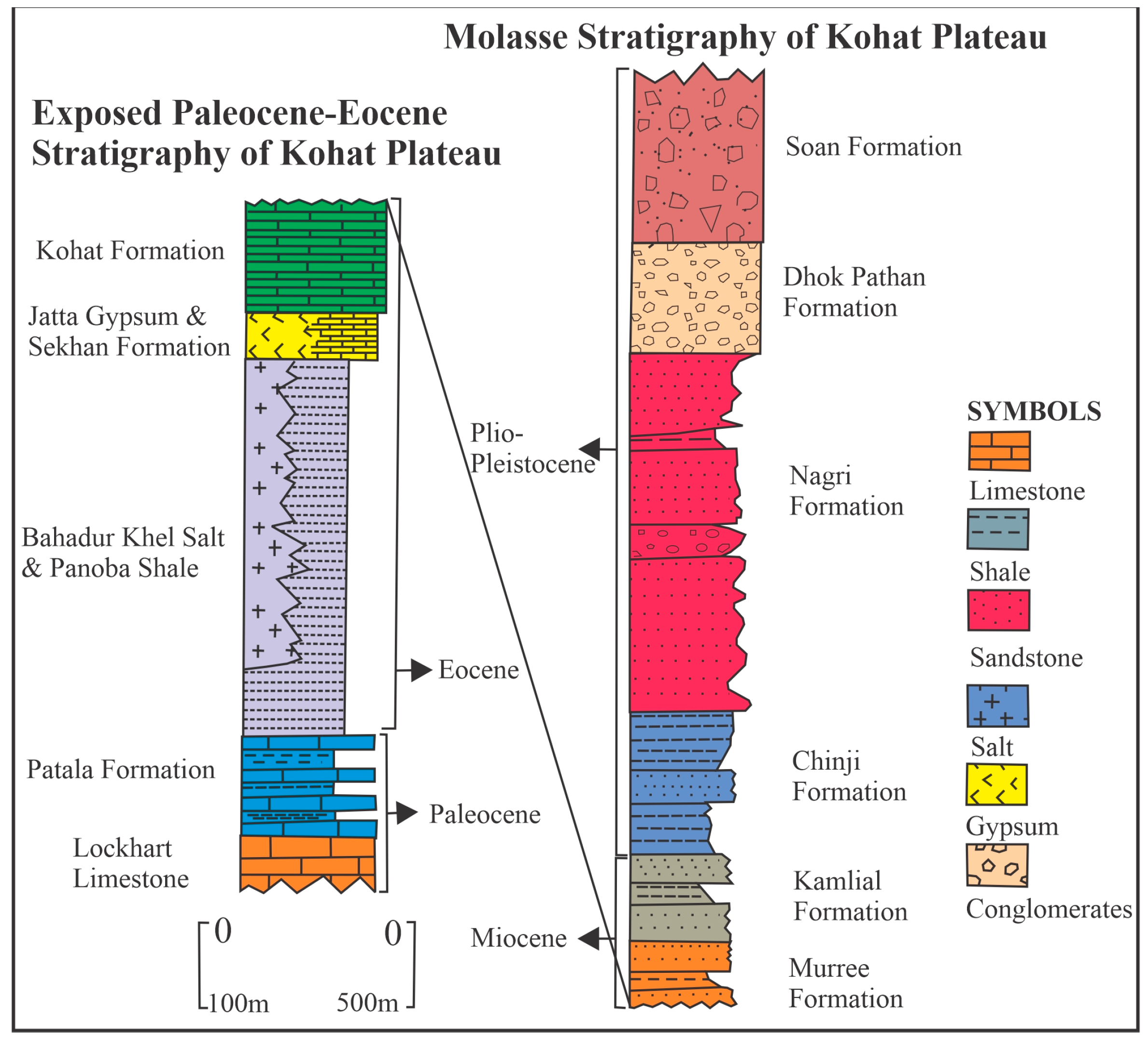
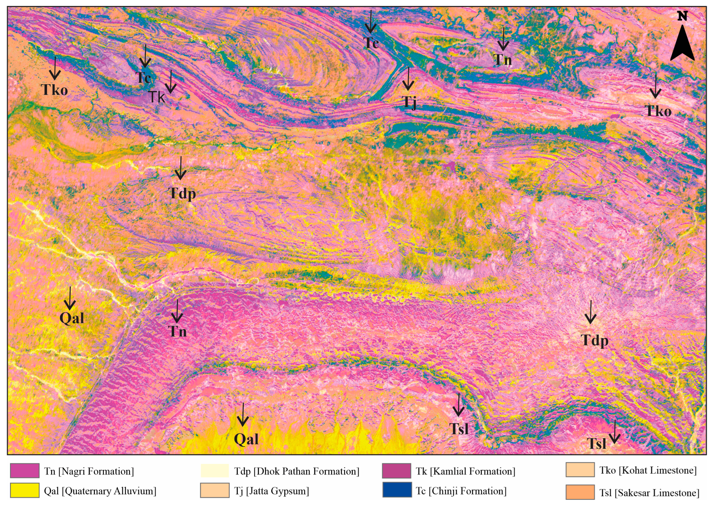
2. Geological Background

The Himalayan mountain range is surrounded by the Indian plate in the south and the Eurasian plate in the north. The Main Mantle Thrust (MMT) represents the boundary formed during the Eocene collision between the Indian plate and the Kohistan–Ladakh arc [20]. The Himalayan deformation migrates southward from the Main Mantle Thrust (MMT) position, as evidenced by the Main Boundary Thrust (MBT), which causes the northern deformed fold and thrust belt to shift southward over the molasse sediments of the Pothohar and Kohat Plateau [21]. In the northwest of the Himalayan fold–thrust zone, the Kohat Plateau is a site of complicated deformation that directly reflects the compressional tectonics brought on by the India–Eurasian collision [22]. A shallow-dipping basal separation beneath the Kohat Plateau has been identified as the cause of the more severe deformation observed there than on the Pothohar Plateau [23]. In contrast, the Kohat Plateau’s structural geometries and stratigraphic correlations show a complex configuration characterized by tectonic events such as wrenching and thrusting [24,25,26]. Beginning in the early Miocene, this belt serves as the primary hub for the influx of synorogenic sediments. As illustrated in Figure 1B, the southern boundary of this deformed fold and thrust belt is produced by the Salt Range Thrust (SRT) and the Trans-Indus Ranges Thrust (TIRT) [27].

Paleocene-to-Pliocene sedimentary strata make up the Kohat Foreland Fold and Thrust Belt. By the early Miocene, these strata had joined the terrigenous Indo-Gangetic foreland basin. Paleocene sandstone, limestone, and shale are the oldest exposed rocks in the area. Because of the pressure of the Indian plate’s edge, these rocks were deposited in a limited fore-deep marine environment and offer the earliest evidence of Himalayan convergence [20]. A complex collection of shale, carbonate, evaporite, and clastic rocks that were deposited in a limited marine basin lies conformably on top of this series. Between the southern Asian edge and the northwest Indian continental margin, these rocks form a tectonically isolated region of the Tethys Sea [20]. The Eocene series is unconformable with the thick succession of molasse sediments from the Miocene to the present day that are found in the Murree and Siwalik Groups. The molasse interval’s lithological constituents include conglomerates, sandstone, and shale. Exhumation in the Himalayas is thought to be the cause of this depositional pattern.

Geologically, the ZY1-02D study area is primarily composed of the Paleocene sequence, the Eocene sequence, the Rawalpindi Group, the Siwalik Group, and Quaternary deposits. The main deformational front of the Kohat Plateau is the Surghar Range, which is situated southeast of it. It reveals Triassic to Eocene rocks, such as carbonates, sandstone, and shale, which are roughly 1100 m thick. Terrigenous Miocene deposits exist on top of the Eocene carbonate and shale strata, which comprise the northern Kohat Plateau’s stratigraphy. The Eocene shelf sediment succession includes the Panoba Shale (Tp), the Kuldana Formation/Mami Khel Clays (Tmk), and the Kohat Formation (Tko) [20,22]. In the Miocene sedimentary rocks, the Rawalpindi Group consists of clastic sediments from the Murree (Tm) and Kamlial (Tk) Formations, which were derived from the ongoing rise of the Himalayan orogeny [23]. Overlying this series, unconformably, are the middle Miocene-to-Pleistocene rocks of the Siwalik Group, forming a dense succession. The Plio-Pleistocene consists of the Siwalik Group, and the strata are distributed in the northeastern and northwestern parts of the study area, with the main lithological units being conglomerate, sandstone, limestone, shale, gypsum, and salt, as shown in Figure 2. The conglomerate contains clasts of metamorphic and igneous rocks in the study area. Furthermore, the Kohat–Pothohar Plateau is regarded as a geological site rich in oil and gas, as well as in several mineral deposits, such as the Siwaliks of the Plio-Pleistocene which contain uranium and paleoplacers of gold deposits, as well as the Paleocene and Eocene which comprise coal, gypsum, and salt deposits [28,29,30]. To the southwest, the plateau is bordered by the relatively flat Bannu Basin, which is covered by recent deposits. The north–south-trending Sulaiman Range, a complex collection of Mesozoic to recent deposits and sedimentary melange, has a faulted contact with the plateau’s western edge.

3. Materials and Methods

3.1. Hyperspectral Images

Two ZY1-02D HSI scenes of the Kohat–Pothohar Plateau were acquired on 5 September 2023. The ZY1-02D data have 166 bands with 30 m spatial resolution and cover the spectral range of 395.86 to 2501.08 nm, as shown in Table 1 [13,19]. The two scenes were geometrically corrected Level 2 radiance data, which were converted from the Level 1 product (digital number) using radiometric calibration data from the China Center for Resources Satellite Data. The full width at half maximum (FWHM) of the VNIR and SWIR data was 8.42 and 16.26 nm, respectively.

The ZY1-02D HSI scenes of the Central Indus Basin in the Surghar Range of the Kohat–Karak region of Khyber Pakhtunkhwa (KPK), Pakistan (between 33°23N–32°58N and 70°51E–71°36E), feature terrain primarily consisting of exposed mountains. This area is a mountainous region with an average altitude of 600 m, characterized by a plateau temperate semiarid climate, with mostly exposed bedrock.

In the original HSIs, using ENVI software 5.6, areas with good exposure were selected, the average spectral characteristics of lithological units with the same lithology were calculated, and the spectral curves of these lithological units were obtained, as shown in Figure 3b. The results indicate that the overall spectral curve shapes of the lithological units are basically consistent, but there are slight differences in the performance of absorption and reflection peaks. Specifically, the seven lithological units have strong reflection characteristics near 500 nm in the near-infrared spectrum and near 1600 nm and 2100 nm in the far-infrared spectrum, as well as strong absorption characteristics near 650 nm and 2300–2350 nm. The reason can be attributed to the mixed spectra generated by intense weathering and erosion. Among them, the limestone of the Paleocene and Eocene sequences has obvious reflection characteristics in the 2000–2150 nm. Other sedimentary rocks can also be distinguished by their reflection and absorption characteristics of different intensities, indicating that hyperspectral classification methods can be used for classification. The strata in this study area mostly dip northwest–southeast. The geological map of the ZY1-02D study area is shown in Figure 1C.

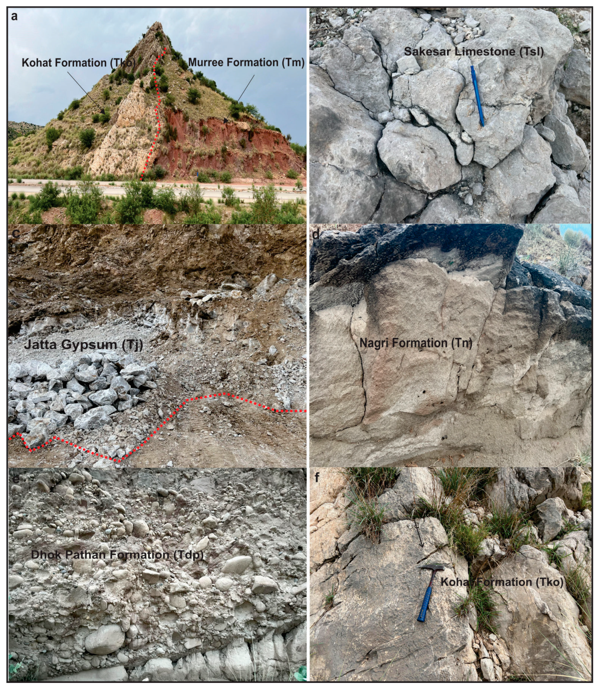
3.2. Field Validation

A field campaign and sample analysis in the laboratory confirmed the accuracy of the mapping techniques. By measuring the reflectance of both fresh and weathered sample surfaces, the spectral characteristics of these samples were evaluated. All lithological units in the research region were represented in the 41 rock samples that were gathered from 24 different locations. Twenty-two samples were taken from the west side, nineteen samples—from the east side of the HSI image scenes in the Kohat–Pothohar Plateau.

Reflectance spectra of the collected samples were measured in the laboratory using a Spectral Evolution/SR-3500TM spectroradiometer (350–2500 nm) with a 2 cm field of view and a contact probe containing an internal halogen lamp. The radiance spectrum was converted to reflectance using a Spectralon^TM white panel. Twenty-seven random spots were measured for each sample (weathered and fresh surfaces), with an average of 20 co-adds for each spot, and spectra from all spots were averaged to create a representative spectrum for each sample.

3.3. Hyperspectral Data Preprocessing

The radiance of the ZY1-02D data was atmospherically corrected to surface reflectance using the Fast Line-of-sight Atmospheric Analysis of Spectral Hypercubes (FLAASH) model [31] with the following parameters: 778 km sensor altitude, water absorption feature centered at 1135 nm, rural aerosol model, and 40 km initial visibility without spectral polishing. The ground elevation was set on the basis of the ASTER Ground Digital Elevation Model (GDEM) data at 30 m grids. To avoid the influence introduced by the incorrectly estimated amount of water vapor using the FLAASH water vapor model, the parameters of the atmospheric model were determined based on the average water vapor values derived from the Moderate Resolution Imaging Spectroradiometer (MODIS) MOD05_L2 precipitable water vapor data acquired about 25 min after the ZY1-02D data acquisition [32]. Spectra from the same target within the overlapping areas between adjacent scenes were compared to make sure the radiometric correction results were consistent across both scenes. The spectral features (absorption positions and depths) from the same target were comparable for the adjacent data sets due to the extremely arid meteorological conditions (less than 102 mm annual rainfall) [13].

The overlapping bands of the VNIR and SWIR sensors and the bands of water vapor absorption were excluded, and 129 bands were retained, including bands 3~66 (413.04~954.24 nm), 78~97 (1022.21~1341.16 nm), 107~124 (1509.54~1795.43 nm), and 139~166 (2048.13~2484.33 nm). Both scenes were geo-referenced to the same map projection using a local datum, and a mosaic of the ZY1-02D reflectance data was generated, covering most of the study area.

Instead of using a single large spectral band, hyperspectral imagers together collect the scene image in several narrow spectral bands. The spatial resolution of a hyperspectral imager is usually lower than that of multispectral and panchromatic imagers due to the extremely narrow spectral band of a channel. As Table 1 illustrates, many hyperspectral imagers consist of two spectrometers: one for the VNIR (400–1000 nm) band and the other for the SWIR (900–2500 nm) band. A hyperspectral sensor’s signal-to-noise ratio (SNR), which measures the signal’s strength in contrast to background noise, provides insight into the quality of the data it collects. The sensor’s capacity to identify small spectral characteristics and differentiate between materials is affected directly by the SNR. The accuracy and quality of hyperspectral image analysis are greatly influenced by the signal-to-noise ratio (SNR). In addition to the hyperspectral sensors’ ability to record spectral information in hundreds of tiny bands, even minute levels of noise may affect the quality of the data and cause results to be misinterpreted. The noise characteristics that are present in hyperspectral sensors includes dark noise, which is caused by thermally produced electrons in the detector, and shot noise, which results from the statistical variance of photon arrivals and is more noticeable in low-light conditions [33].

3.4. Spectral Feature Identification

According to the alteration appearances of lithological units, the laboratory spectra of minerals, including kaolinite, illite, quartz, gypsum, muscovite, chlorite, and calcite, were extracted from the USGS spectral library to recognize the spectral features of the alteration in the working area to monitor the understanding of sample spectra and assist further hyperspectral mapping [34]. Each of the seven minerals shows diagnostic absorption features in the SWIR region with different absorption wavelengths (center) and strengths [35]. The limestone alteration exhibits absorption features around 2250 and 2350 nm induced by Co₃⁺² [36]. The advanced argillic alteration is characterized by kaolinite and alunite; kaolinite shows the diagnostic Al-OH features near 2165 and 2200 nm, whereas alunite has a strong absorption feature at 2170 nm and a weak absorption feature at 2320 nm caused by Al-OH [37].

All USGS spectra and laboratory spectra from the field samples were resampled to the 166 bandpass of the preprocessed ZY1-02D data (Figure 3) to test if the diagnostic spectral features preserved their spectral shape (slope, band position, and band depth) when resampled to the satellite sensors at a coarser spectral resolution. Figure 3a indicates that minor and narrow features (e.g., 2165 nm absorption for kaolinite) are becoming relatively weaker after resampling. However, the overall spectral shape and dominant spectral feature positions are comparable before and after resampling. This means that the selected USGS reference spectra can be used as end members in search for similar signatures in satellite data to facilitate feature identification and hyperspectral data processing.

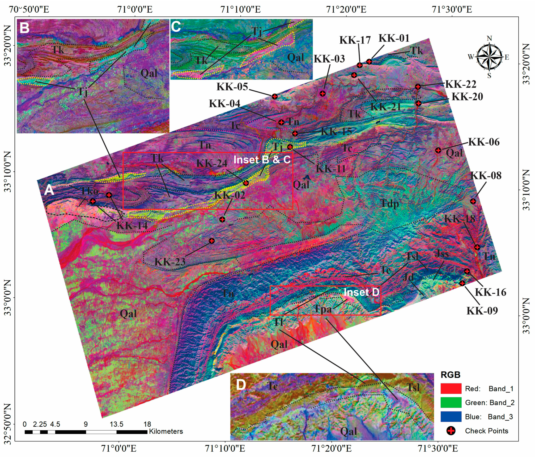
3.5. False Color Composite of Surface Reflectance

False color composite images can be used to enhance and reveal important lithological differences and alteration zones [10,11,32]. The false color composite of three bands, i.e., 116, 148, and 156 (1644.0, 2199.48, and 2334.19 nm) in red, green, and blue (RGB) spectral channels can enhance the visual representation of rocks with limestone and gypsum alteration. The Earth’s surface is frequently decrypted using several color combinations of satellite images obtained in the VNIR, SWIR, and TIR spectral bands. Using an additive RGB model, FCC is among the finest methods for interpreting raster data acquired in various electromagnetic spectrum ranges (both visible and invisible) [38]. The primary purpose of color composites from the Landsat data collection is to identify different kinds of geological elements, including rocks, vegetation, and water bodies [39,40]. A false color composite (FCC) is made for lithological mapping by combining a number of spectral channels that are collectively less correlated and represent distinct spectral properties of absorption and reflection of various rocks and minerals [41]. The received spectral channel combinations allow for the separation of areas with distinct minerals, lithological variations, and structures, which are represented by varying colors and gradients on the resulting FCC image [39]. The same combination’s color spectrum may vary depending on the region under study, which is influenced by the various sedimentation conditions and rock mineral compositions [42]. For the framework of our study, a false RGB composite from 116, 148, and 156 bands of the ZY1-02D data was selected, which is the most informative for regional mapping of different geological formations within the Kohat–Pothohar Plateau.

3.6. Principal Component Analysis (PCA)

PCA is a statistical technique that creates “principal components” (PCs), which are sets of uncorrelated linear data, from a set of correlated data [23,43]. Both covariance and correlation matrices may serve as its foundation [44,45]. Based on the spectral characteristics of materials found on the Earth’s surface by remote sensing, PCA is frequently used for geological and mineralogical mapping [46]. The data collection that is converted using this method generally retains up to 97% of its original information [47]. This transformation’s primary goal is to improve the signal-to-noise ratio for more accurate Earth’s surface object selection.

The ten channels of the ZY1-02D hyperspectral data have uncorrelated linear combinations (eigenvector loads) that include information about the minerals (biotite, quartz, chlorite, ferrihydrite, calcite, gypsum, etc.). This information can be extracted from near-infrared (VNIR) and shortwave infrared (SWIR) spectral channels [44,45,46]. Generally, PCs with high eigenvector loads in certain spectral channels describe the absorbing and reflecting capabilities of the mentioned minerals with opposite signs. While the negative load in the spectral channel represents the group of minerals as dark pixels, the positive load highlights the group of minerals as bright pixels [48,49].

Using a covariance matrix, ten bands were used to process the PCA approaches for the demarcation of lithological units after PCA was applied to the ZY1-02D remote sensing data.

Table 2. Eigenvectors of the PCA bands of the ZY1-02D HSI data.

Eigenvector	Band 1	Band 2	Band 3	Band 4	Band 5	Band 6	Band 7	Band 8	Band 9	Band 10	Variance, %
PCA1	−0.1966	−0.1963	−0.1961	−0.1960	−0.1958	−0.1957	−0.1955	−0.1953	−0.1951	−0.1950	99.97
PCA2	−0.1193	−0.1358	−0.1363	−0.1340	−0.1320	−0.1249	−0.1191	−0.1130	−0.1075	−0.1012	0.020
PCA3	−0.0601	−0.0147	−0.0095	−0.0129	−0.0121	−0.0345	−0.0521	−0.0721	−0.0890	−0.1072	0.002
PCA4	−0.3830	−0.3033	−0.2591	−0.2204	−0.1737	−0.1457	−0.1144	−0.0872	−0.0651	−0.0409	0.000122
PCA5	0.1662	0.1232	0.1066	0.0925	0.0733	0.0611	0.0450	0.0302	0.0161	0.0019	0.000077
PCA6	0.8369	−0.0844	−0.1297	−0.1564	−0.1517	−0.1498	−0.1548	−0.1635	−0.1704	−0.1613	0.000030
PCA7	−0.1136	0.0804	0.0598	0.0405	0.0244	0.0086	0.0005	−0.0093	−0.0259	−0.0477	0.0000162
PCA8	0.2319	−0.4619	−0.1869	−0.0866	−0.0196	0.0483	0.0933	0.1347	0.1804	0.2236	0.000011
PCA9	0.0292	−0.4789	−0.0659	−0.0057	0.0372	0.0829	0.1072	0.1293	0.1470	0.1653	0.000007
PCA10	0.0053	0.1496	−0.0532	−0.0405	−0.0229	−0.0220	−0.0277	−0.0246	−0.0238	−0.0186	0.00003

provides the eigenvector matrix and covariance eigenvalues of the PCA employing all ten bands. PCA1, PCA2, and PCA3 show values for the ZY1-02D data eigenvectors. The variance was 99.97% according to PCA1’s eigenvalues, 0.020% according to PCA2, and 0.002% according to PCA3’s (Table 2). Consequently, the RGB composite approach of PCA1, PCA2, and PCA3 was the most effective technique for the selected lithological units.

3.7. Support Vector Machine

SVM is a supervised machine learning technique for applications involving regression and classification [50]. SVM, which is based on the statistical learning theory, has proven to be reliable and effective over time. Creating a dividing hyperplane that maximizes the geometric margin between the input samples is the basic idea behind support vector machines (SVMs). SVM streamlines the classification process by mapping the dataset into a higher-dimensional feature space [51]. Notably, SVM has been successfully applied to classify rocks [52]. SVM is the simplest form of a binary classifier, and it can combine multiple binary SVM classifiers into a multiclass classifier [1]. It has generated significant interest in the remote sensing community, especially in lithological mapping.

The SVM algorithm has a number of benefits, including the capacity to manage high dimensionality and small sample sizes. Because of this, it is a dependable and precise classifier for lithological mapping in applications involving remote sensing. SVM is an effective machine learning technique that has transformed spectral-based lithological mapping and is widely utilized because of its speed and accurate findings [53].

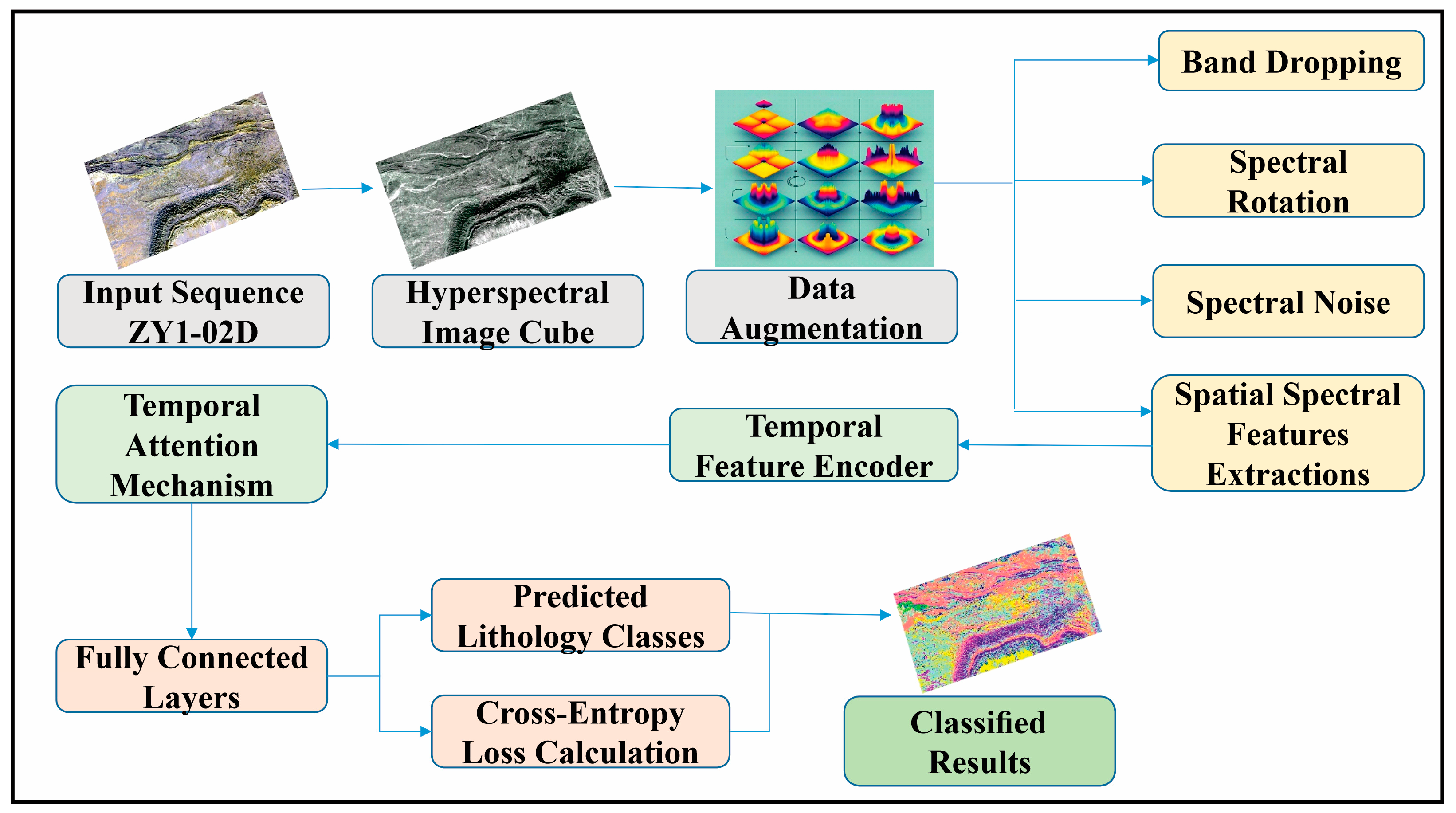
3.8. Spatial–Spectral Transformer (SSTF)

For lithological classification, a spatial–spectral transformer (SSTF) has been suggested. In a variety of applications, SSTF, a deep learning technique known as a “transformer,” has shown strong performance [54,55]. In contrast to convolutional and recurrent neural networks, the transformer network is based entirely on a self-attention process and employs encoder and decoder architecture. The encoder and decoder layers are constructed using the same architecture, and the image is treated as sequence data. The input data are transformed into sequence representations with position information by the encoder, and the output sequence is then created by the decoder. An attention system that automatically modifies the relationship between various locations and concentrates on the areas that need attention connects the encoder and the decoder. In order for the network to create a feature map for each class, the attention mechanism’s main function is to modify the weights for pixel classification.

To represent the long-range dependence between input and output, a function matrix was computed in the form of vectors using the following steps:

For the input sequence [56], the hyperspectral data cube is represented as follows:

$$\mathrm{X}\in {\mathrm{R}}^{\mathrm{H}\times \mathrm{W}\times \mathrm{B}}$$

(1)

where R is the hyperspectral data cube, H is the height, W is the width, and B is the spectral band.

The cube is divided into spatial–spectral patches or sequences. A patch is represented as follows:

$${\mathrm{X}}_{\mathrm{t}}\in {\mathrm{R}}^{\mathrm{K}\times \mathrm{K}\times \mathrm{B}}$$

(2)

where K is the spatial patch size.

Spatial–spectral features are extracted using 3D convolutions, which extract features from the spatial and spectral dimensions:

$${\mathrm{F}}_{\mathrm{s}\mathrm{p}\mathrm{a}\mathrm{t}\mathrm{i}\mathrm{a}\mathrm{l}-\mathrm{s}\mathrm{p}\mathrm{e}\mathrm{c}\mathrm{t}\mathrm{r}\mathrm{a}\mathrm{l}}=\mathrm{C}\mathrm{o}\mathrm{n}\mathrm{v}3\mathrm{D}\left(\mathrm{X}\right)$$

(3)

This transforms the cube into spatial–spectral embedding:

$${\mathrm{F}}_{\mathrm{s}\mathrm{p}\mathrm{a}\mathrm{t}\mathrm{i}\mathrm{a}\mathrm{l}-\mathrm{s}\mathrm{p}\mathrm{e}\mathrm{c}\mathrm{t}\mathrm{r}\mathrm{a}\mathrm{l}}\in {\mathrm{R}}^{{\mathrm{H}}^{\prime }\times {\mathrm{W}}^{\prime }\times \mathrm{D}}$$

(4)

where ${\mathrm{H}}^{\prime }$ and ${\mathrm{W}}^{\prime }$ are the reduced spatial dimensions and D is the depth of the extracted features.

3.8.1. Data Augmentation: Spectral Noise, Spatial Rotation, and Band Dropping

Data augmentation is a technique to artificially expand the training dataset by applying various transformations to the input data as shown in Figure 4. For hyperspectral images, these transformations are designed to enhance the model’s ability to generalize across variations in the data, especially for lithology prediction tasks. Below is a detailed explanation of the three augmentation techniques: spectral noise, spatial rotation, and band dropping.

• Spectral noise: adding noise to the spectral bands simulates real-world scenarios where hyperspectral data may contain noise due to sensor limitations or environmental conditions.

Mathematical explanation: if $\mathrm{X}\in C$ is the original hyperspectral data cube, then spectral noise can be modeled as follows:

$${\mathrm{X}}_{\mathrm{n}\mathrm{o}\mathrm{i}\mathrm{s}\mathrm{y}}=\mathrm{X}+\mathrm{N}$$

where ${\mathrm{X}}_{\mathrm{n}\mathrm{o}\mathrm{i}\mathrm{s}\mathrm{y}}$ is the augmented data cube with added spectral noise; N ∈ ${\mathbb{R}}^{(\mathrm{H}\times \mathrm{W}\times \mathrm{B})}$ is the noise matrix, where ${\mathrm{N}}_{\mathrm{i},\mathrm{j},\mathrm{k}}\sim \mathcal{N}(\mathsf{\mu },\mathsf{\sigma }2)$; μ is the mean of the noise (often 0); and σ² is the variance of the noise, controlling its intensity.

2.

Spatial rotation: rotating the spatial dimensions of the hyperspectral data simulates variations in orientation that might occur during data acquisition.

Mathematical explanation: let $\mathrm{X}\in {\mathbb{R}}^{(\mathrm{H}\times \mathrm{W}\times \mathrm{B})}$ represent the hyperspectral cube, where each slice $X_{(\colon\colon b)}\in {\mathbb{R}}^{(\mathrm{H}\times \mathrm{W})}$ corresponds to the bth spectral band. Spatial rotation applies rotation matrix R to the spatial dimensions:

$${\mathrm{X}}_{\mathrm{r}\mathrm{o}\mathrm{t}\mathrm{a}\mathrm{t}\mathrm{e}\mathrm{d}}=\mathrm{R}\times \mathrm{X}$$

where R is the 2D rotation matrix, defined as R = [cosθ -sinθ; sinθ cosθ] and θ as the angle of rotation (e.g., 90°, 180°, 270°).

The rotation is applied consistently across all spectral bands to maintain spatial coherence.

3.

Band dropping: band dropping randomly removes certain spectral bands to simulate scenarios where specific wavelengths may be missing or corrupted, ensuring the model learns to handle incomplete data.

Mathematical explanation: let $\mathrm{X}\in {\mathbb{R}}^{\left(\mathrm{H}\times \mathrm{W}\times \mathrm{B}\right)}$ be the original hyperspectral cube, and let $\mathrm{M}\in {\mathbb{R}}^{\left(\mathrm{B}\right)}$ be a binary mask vector, where $M_b=1$ if band b is retained and 0 if band b is dropped.

The augmented data cube is then as follows:

$${\mathrm{X}}_{\mathrm{d}\mathrm{r}\mathrm{o}\mathrm{p}\mathrm{p}\mathrm{e}\mathrm{d}}=\mathrm{X}\odot \mathrm{M}$$

where ⊙ is the element-wise multiplication along the spectral dimension and M is sampled in such a manner that a predefined proportion of bands is dropped (e.g., 10–20%).

3.8.2. Combined Effect

By applying these augmentations, spectral noise improves robustness to noise in sensor data, spatial rotation ensures invariance to orientation differences, and band dropping enhances the model’s ability to deal with missing spectral information.

The resulting augmented dataset contains variations of X, represented as follows:

$${\mathcal{D}}_{\mathrm{a}\mathrm{u}\mathrm{g}\mathrm{m}\mathrm{e}\mathrm{n}\mathrm{t}\mathrm{e}\mathrm{d}}=\{{\mathrm{X}}_{\mathrm{n}\mathrm{o}\mathrm{i}\mathrm{s}\mathrm{y}},{\mathrm{X}}_{\mathrm{r}\mathrm{o}\mathrm{t}\mathrm{a}\mathrm{t}\mathrm{e}\mathrm{d}},{\mathrm{X}}_{\mathrm{d}\mathrm{r}\mathrm{o}\mathrm{p}\mathrm{p}\mathrm{e}\mathrm{d}},\dots \}$$

These augmentations are typically applied stochastically during training, ensuring that the model observes diverse input scenarios.

The temporal feature encoder feeds sequential spectral embedding into a BiLSTM or Transformer. The temporal output for each sequence is as follows:

$${\mathrm{F}}_{\mathrm{t}\mathrm{e}\mathrm{m}\mathrm{p}\mathrm{o}\mathrm{r}\mathrm{a}\mathrm{l}}=\mathrm{B}\mathrm{i}\mathrm{L}\mathrm{S}\mathrm{T}\mathrm{M}\left({\mathrm{F}}_{\mathrm{s}\mathrm{p}\mathrm{a}\mathrm{t}\mathrm{i}\mathrm{a}\mathrm{l}-\mathrm{s}\mathrm{p}\mathrm{e}\mathrm{c}\mathrm{t}\mathrm{r}\mathrm{a}\mathrm{l}}\right)$$

(5)

$${\mathrm{f}}_{\mathrm{t}}=[{\mathrm{h}}_{\mathrm{t}}^{\to };{\mathrm{h}}_{\mathrm{t}}^{\leftarrow }]$$

where ${\mathrm{h}}_{\mathrm{t}}^{\to }$ are the forward and ${\mathrm{h}}_{\mathrm{t}}^{\leftarrow }$ are the backward LSTM outputs.

The temporal attention mechanism computes attention scores to focus on important spectral regions:

$${\propto }_{\mathrm{t}}=\mathrm{e}\mathrm{x}\mathrm{p}{\displaystyle \frac{{\mathrm{w}}^{\mathrm{t}}{\mathrm{f}}^{\mathrm{t}}}{\sum {\mathrm{t}}^{\prime }\mathrm{e}\mathrm{x}\mathrm{p}\left({\mathrm{w}}^{\mathrm{t}}{\mathrm{f}}^{\mathrm{t}}\right)}}$$

(6)

The attended features are as follows:

$$\mathrm{C}={\sum }_{\mathrm{t}}{\propto }_{\mathrm{t}}{\mathrm{f}}_{\mathrm{t}}$$

where C is the attended features (context vector), $\propto$ is the computed attention score, t is the time, $w^t$ is the learnable weight → w ∈ $R^d$, $R^d$ is the dimensionality data (extent of the importance given in the training data), $w^t{f}^t$ computes the dot product between the weight w and the vector temporal $f^t$, resulting in a scalar score for each time step. Exponentiation ensures the attention score is positive.

Fully connected layers aggregate features via dense layers to predict lithology classes [57]:

$${\mathrm{y}}_{\mathrm{p}\mathrm{r}\mathrm{e}\mathrm{d}}=\mathrm{s}\mathrm{o}\mathrm{f}\mathrm{t}\mathrm{m}\mathrm{a}\mathrm{x}\left(\mathrm{W}\mathrm{c}+\mathrm{b}\right)$$

(7)

where ${\mathrm{y}}_{\mathrm{p}\mathrm{r}\mathrm{e}\mathrm{d}}\in {\mathrm{R}}^{\mathrm{c}}$, c is the number of lithology classes, and b is the bias.

Definition of Softmax [58]:

$$\mathrm{S}\mathrm{o}\mathrm{f}\mathrm{t}\mathrm{m}\mathrm{a}\mathrm{x}\left(\mathrm{Z}\mathrm{i}\right)={\displaystyle \frac{\mathrm{e}\mathrm{x}\mathrm{p}\left(\mathrm{Z}\mathrm{i}\right)}{{\sum }_{\mathrm{j}=1}^{\mathrm{c}}\mathrm{e}\mathrm{x}\mathrm{p}\left(\mathrm{Z}\mathrm{i}\right)}}$$

(8)

Loss function (cross-entropy loss) for each predicted pixel or patch is calculated as follows:

$$\mathcal{L}=-{\displaystyle \frac{1}{\mathrm{N}}}{\sum }_{\mathrm{i}=1}^{\mathrm{N}}{\sum }_{\mathrm{c}=1}^{\mathrm{c}}\mathrm{y}\mathrm{i},\mathrm{c}\mathrm{l}\mathrm{o}\mathrm{g}({\mathrm{y}\mathrm{i}}^{^},\mathrm{c})$$

(9)

where $\mathcal{L}$ is the loss, N is the number of training samples, c is the number of classes, ${yi}^{^} \mathrm{a}\mathrm{n}\mathrm{d} c$ are the binary indicators, and ${yi}^{^},c$ is the predicted probability for class c. The logarithm amplifies the penalty for incorrect predictions by making it larger when the model assigns low probability to the correct class.

Optimization uses the Adam optimizer to minimize the loss:

$${\mathsf{\theta }}_{\mathrm{i}+1}={\mathsf{\theta }}_{\mathrm{t}}-\mathrm{ղ}.\nabla \mathcal{L}\left({\mathsf{\theta }}_{\mathrm{t}}\right)$$

(10)

where $\mathrm{ղ}$ is the learning rate, $\theta$ represents the model’s parameters, $\nabla$ is the gradient operator used to compute the vector of partial derivatives of a function with respect to its parameters, and $\nabla \mathcal{L}\left({\mathsf{\theta }}_{\mathrm{t}}\right)$ is the gradient of the loss function with respect to the parameters.

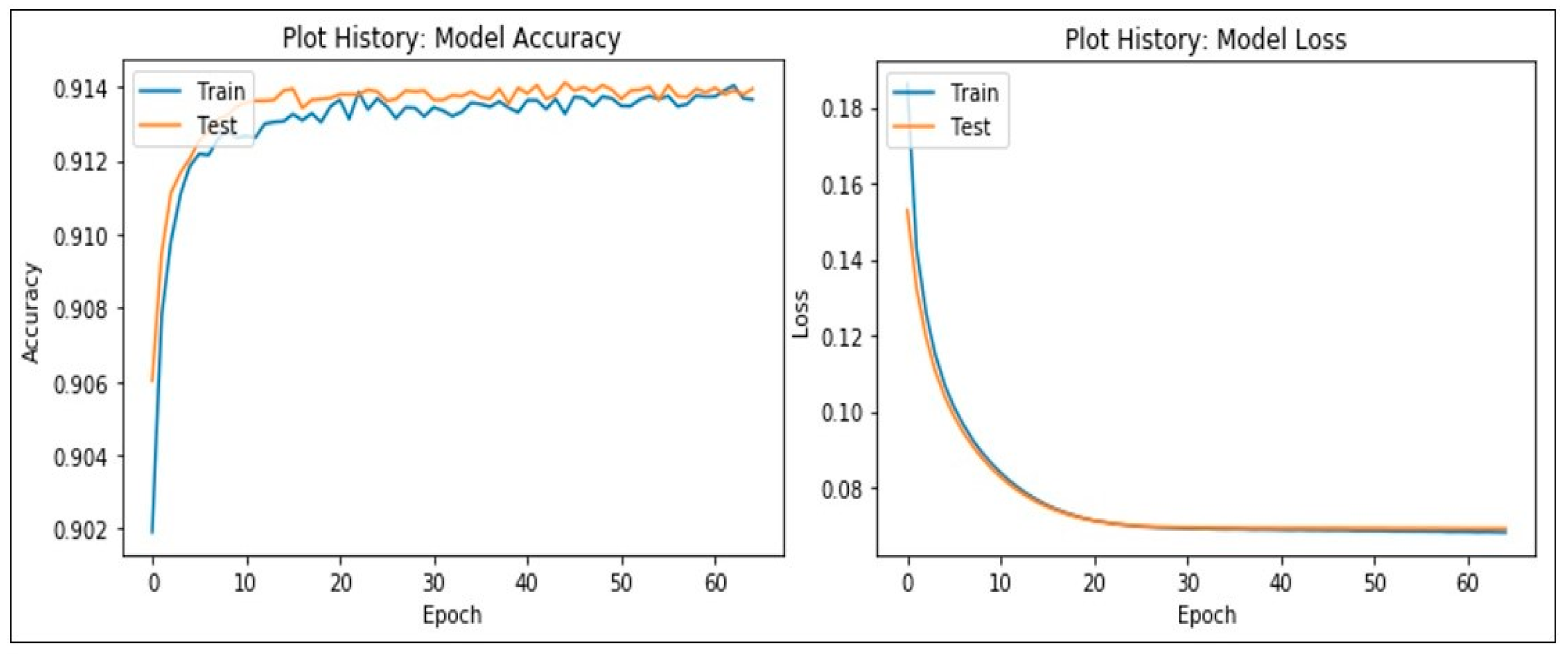
3.9. Accuracy Assessment

Overall accuracy (OA), average accuracy (AA, which is calculated by averaging the user accuracy and the producer accuracy), and the Kappa coefficient (KC), which is derived from a confusion matrix, were used to assess the lithology mapping results from SVM and SSTF. The probability that the classifier correctly labels image pixels is represented by producer accuracy, and the probability that the classifier correctly assigns pixels to their predefined classes is represented by user accuracy. OA is calculated as the ratio of correctly classified pixels (diagonal elements of the confusion matrix) to the total number of test pixels. By considering the complete contingency matrix and offering a metric of result agreement that goes beyond OA, the KC evaluates the consistency between the classification map and the reference data. The purpose of this assessment is to evaluate the efficacy of classification methods for lithological mapping in the study area and estimate the classification results from different methods and datasets.

4. Results

4.1. False Color Composite of Surface Reflectance

The false color composite for the research area is shown in Figure 5 at 1644.01 nm (R), 2199.48 nm (G), and 2334.19 nm (B). It provides an overview of how various kinds of major alteration are distributed. The absorption features of ${\mathrm{F}\mathrm{e}}^{2+}$ and Al-OH are located in bands 1644.01 and 2199.48 nm, respectively, while the absorption features of Fe, Mg-OH, and ${\mathrm{C}\mathrm{O}}_3^{2-}$ are located in band 2334.19 nm. As a result, rocks with argillic and phyllic alteration and the Al-OH absorption characteristic at 2200 nm appear pink to red. On Figure 5, calcite-rich rocks are shown in yellow due to their ${\mathrm{C}\mathrm{O}}_3^{2-}$ spectral absorption at 2350 nm.

According to Figure 5, the Kohat–Pothohar regions are where argillic and phyllic alteration is most prevalent. Due to Paleocene sedimentary layers, calcite-rich outcrops are mostly found from east to west and in the southern parts of the study area. The pink-to-red colored known deposits (gypsum) are all associated with phyllic alteration. Two distinct color zones that progressively narrow from east to west enhance the alteration halo of the Kohat–Pothohar deposit. Limestone- and gypsum-altered rocks can be clearly identified by colors on the composite image due to the presence of absorption features and spectral slope variability. The pink appearance of the clay minerals kaolinite and muscovite/sericite is caused by Al-OH absorption (at band 116). Additionally, the significant reflectance of CO₃ at bands 116 and 148 and the strong absorption at band 156 (Figure 3) define the yellow color of the carbonates of the Kohat Formation (Tko).

4.2. Principal Component Analysis (PCA)

For the ZY1-02D remote sensing data, the PCA reveals different lithological units with diverse colors marked by names of lithological units. The Jatta Gypsum (Tj) is delineated in yellow while Kohat limestone (Tko) is in a light pink color as shown in Figure 5. As for a clearer observation of the lithological unit Tj under variation of bands such as band 3, band 2, and band 1, which is displayed in Figure 6B, it is represented in a marine blue color. In addition, band 3, band 1, and band 2, which is revealed in Figure 6C, highlighted Tj in a flat pink color. Similarly, the lithological unit Kamlial Formation (TK), which is delineated in a light brown color across all variations of bands, is shown in Figure 6A–C. Quaternary alluvial deposits (Qal) are spotted in a dotted greenish yellow color, as shown in Figure 5A–C. The Chinji Formation (Tc), which is composed of 70% sandstone and 30% reddish clay, is delineated in pink with a mixture of a marine blue color. The Dhok Pathan Formation (Tdp), which consists of sand and conglomerates, is spotted in light green with a mixture of a dotted pink color. Sakesar limestone (Tsl) and Lockhart limestone (Tl) are delineated in a dark-sea blue color as shown in Figure 6A; furthermore, band 3, band 1, and band 2 show Tsl and Tl in a golden color, as shown in Figure 6D. The Patala shale (Tpa), which is composed of shale, is delineated in a moderate pink color, as shown in Figure 5A,C. The Samana Suk Formation (Jss) is delineated in emerald green, while the Nagri Formation (Tn) is demarcated in a light purple color, as shown in Figure 6A.

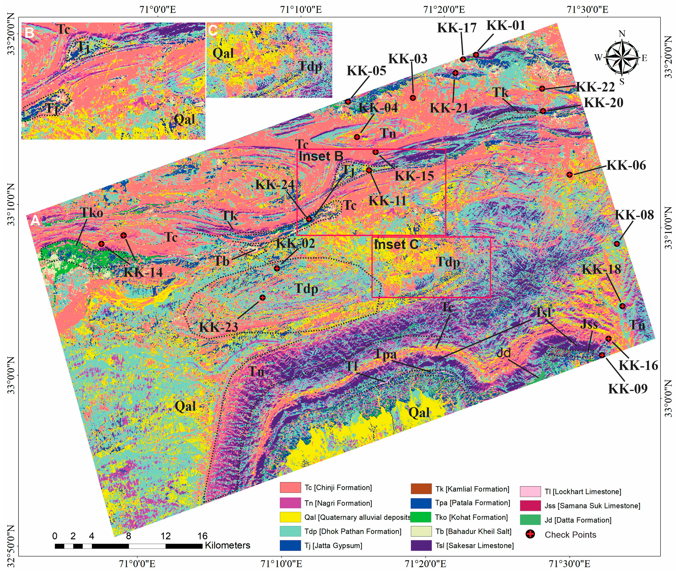
4.3. Support Vector Machine

For lithological mapping using satellite data, the SVM approach offers significant benefits. Results from the ZY1-02D HSI data show that SVM provided good accuracy, with the total accuracy rates ranging from 89.7% with the Kappa coefficient of 0.89. It is highly effective at differentiating between classes and uses comprehensive spectral information of hyperspectral data to achieve accurate classification. SVM presented reliable classification results and mapped the lithological units accurately with limited resources as shown in Figure 7.

4.4. Spatial–Spectral Transformer (SSTF)

We added a block mechanism that enhances the extraction of spectral and spatial information to the transformer in order to make the network more flexible for the high-resolution ZY1-02D HSI data (Figure 8). In contrast to the usual transformer approach, which frequently classifies a spectrum image band-wise, SSTF makes use of the GSE block, which may learn pixel-wise representation and handle the spectral correlation between neighboring bands [59].

While the original geologic map featured 15 rock types (Figure 1C), similar rock types were merged manually to address only compositional variations. Thus, a total of 13 classes were selected as regions of interest. The classification accuracy of each rock type was calculated based on cross-validation, and a confusion matrix was constructed to describe the false alarms among different rock types. Cross-validation of the SSTF method with 20% training pixels produced an overall accuracy of 92.1% and a Kappa coefficient of 0.92 (Figure 9).

4.5. Field Validation

Field inspections were conducted to assess the accuracy of mapping results obtained by the false-color composite, SVM, and SSTF methods. For SVM and SSTF, 40% of the pixels from each category were randomly extracted as training samples, with the remaining pixels used as the test samples, and all were implemented in ENVI 5.6 and Python 3.9, a machine learning and deep learning framework [1].

The results indicate that the machine learning and deep learning models currently used in the ZY1-02D HSI data perform very well in the field of hyperspectral lithology identification. Even with strategies to prevent information leakage applied to the deep learning network models [59], their final classification performance remains more satisfactory than that of traditional machine learning methods.

In order to verify the accuracy of the lithological classification map, we conducted on-site verification of the lithological units within the study area. Figure 10a–f shows field photographs of various types of rocks, which include limestone, sandstone, gypsum, and conglomerates discovered in the ZY1-02D study area. The lithology of the measurement points matches well the predicted lithology of the classification lithology map generated using the SVM and SSTF models. Field verification provides great confidence for HSI classification that relies on geological maps as training labels [5].

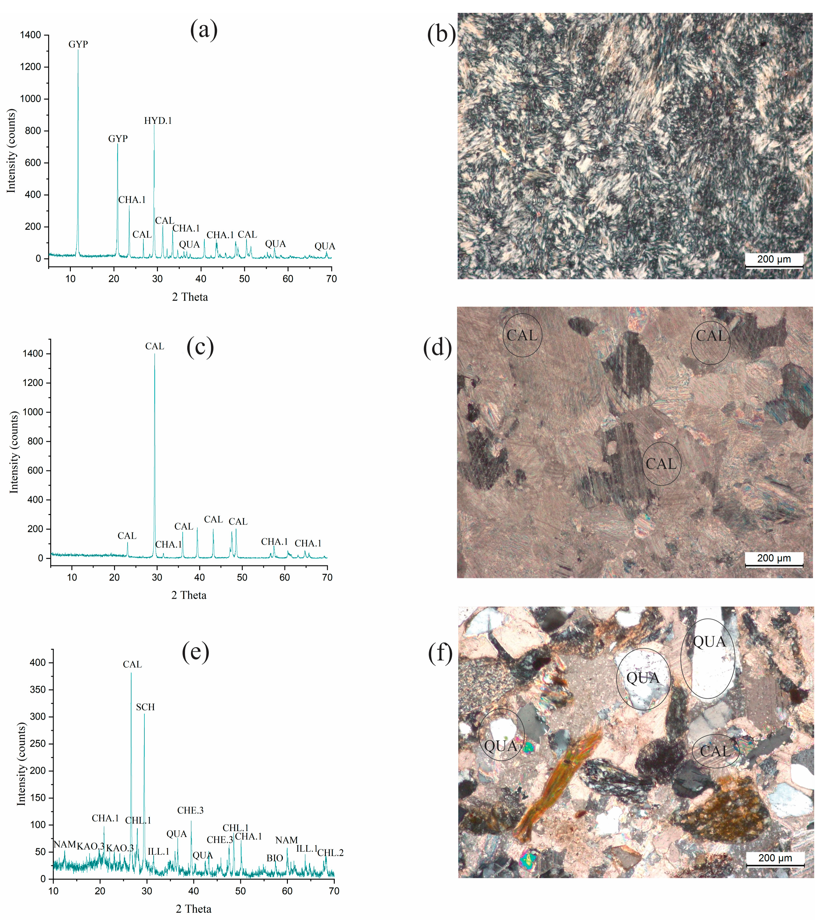
4.6. Relationships Between the Laboratory-Measured Spectra and the Image Spectra

In order to demonstrate the swelling behavior of soils, clay mineralogical compositions are generally determined using conventional laboratory investigations (such as X-ray diffraction and geotechnical analyses), despite the fact that these methods are time-consuming, costly, and slow. Therefore, another approach that could help identify and target expansive soils is needed, as these traditional studies are not well-adapted to large datasets or large-scale investigations.

In this way, reflectance spectroscopy—the study of light reflected from materials—makes it possible to quantify soil qualities quickly and affordably through the examination of reflectance spectra. The montmorillonite, illite, and kaolinite spectra show absorption bands in the shortwave infrared spectral domain (SWIR: 1100–2500 nm) that are caused by vibrational processes that impact water molecules and hydroxyl; these absorption bands can be used to identify these minerals.

A deep and typically asymmetric sharp absorption band at about 1400 nm and a deep absorption band at about 1900 nm are visible in the montmorillonite spectra. At about 2200 nm, there is a distinct absorption band that is shallower than the absorption band at about 1900 nm.

Deep absorption bands can be observed in the illite spectra at about 1400 and 1900 nm, as illustrated in Figure 3a. In general, the absorption band at about 1400 nm is sharper than the absorption band of montmorillonite at around the same wavelength. Compared to the absorption band of montmorillonite at around 1900 nm, the absorption band at this wavelength is shallower. The absorption band at around 2200 nm is crisp, deep, and comparable to the absorption band at about 1900 nm. There are two more shallow absorption bands at 2340 and 2440 nm [60,61,62].

Selecting the best technique for lithological mapping using satellite data requires an understanding of rock mineralogy and spectroscopy [35]. Gathering field sample spectra that can be compared to spaceborne sensor spectra is helpful. Certain types of rocks have poor reflectivity (less than 20%) (Figure 11a–d), which may make matching spectra more challenging. The forms of the laboratory spectra for lithological units are similar to the ZY1-02D data spectra (Figure 3), despite the fact that atmospheric influences, instrument effects, spatial resolution, mixed pixels, and weathering may all have an impact on matching image spectra to laboratory spectra [36,63].

5. Discussion

According to the 1:50,000-scale geologic map, traditional geologic surveys are expensive and sometimes ineffective at mapping small outcrops. High-resolution remote sensing imaging is, therefore, required for planning future research. The mapping of relatively small rock outcrops is made possible by the high spatial resolution of the VNIR and SWIR ZY1-02D data.

Our study’s objective was to determine whether regional geological mapping of the Kohat–Pothohar Plateau could be accomplished using a dataset that included moderate vegetation, a sharply continental climate, and alpha-humus soils that somewhat impact the spectral curve-altered minerals. A cloudless scene with an acquisition date that had the lowest level of humidity and vegetation was used to reduce the adverse environmental effects when performing geological mapping. Statistically reasonable image processing algorithms such as FCC, PCA, SVM, and SSTF were utilized to classify mutually independent image pixels, reduce the correlation between spectral channels, and identify and eliminate hidden limitations to lithological classification.

To determine whether geological mapping of the study area was feasible, the first stage of the study generated a false color composite (FCC) from bands 116, 148, and 156 (1644.0, 2199.48, and 2334.19 nm) in the red, green, and blue (RGB) spectral channels of the ZY1-02D data. Consequently, it was determined that it was impossible to definitively identify rocks or their complexes because of the extremely complex geological structure of the study area, the presence of vegetation cover, thick quaternary sediments, and a similar material composition of the main rock mass. Despite this, based on the spatial distribution, there was a strict separation in sedimentary rocks (Figure 5). Lithological zones containing calcite and other clay minerals were successfully identified using the FCC technique [35,36] (Figure 5). In addition, on the basis of landscape and structural–geomorphological conditions, colors and gradient transitions of the false RGB image, spatial distribution of groups of altered minerals, limestone, gypsum, and Quaternary deposit areas were identified, mapped according to the geological map [64].

In the second phase of the study, the ZY1-02D data were statistically processed using the PCA technique, and a correspondence between its components and groups was established based on the analysis of eigenvector matrices and the creation of two-dimensional correlation plots. The results of the transformation created an RGB composite, which is unique and in its own way reflects the geological and morphological conditions of the study area. The two-dimensional correlation plots show a strong linear trend (Figure 6), and the eigenvector matrices contain loads that are high enough for the selected bands (Table 2).

PCA and FCC are beneficial for initial data exploration since they are excellent at reducing dimensionality and visualizing complex datasets in a more interpretable form. These approaches help in highlighting important variations that can subsequently be examined further using advanced classification techniques. They are useful for reducing the dataset before using advanced classifiers since they can effectively reduce noise and assist in finding the most important spectral components.

PCA implies linearity in data, which may not always be the case in geological mapping where non-linear correlations are typically present. This can restrict its ability to capture complex geological features accurately. Although FCC is capable of visually highlighting distinct lithological units, it might not yield as precise or dependable classification results as machine learning techniques, especially in regions with more subtle variations or substantial spectrum overlap.

PCA and FCC are more suitable for exploratory data analysis and identifying broad trends in the data, but they are less successful at classifying data with high accuracy in complex geological contexts, where advanced classifiers such as SVM and SSTF are required.

For lithological mapping, the best machine learning and deep learning methods in the third phase of the study were SVM and SSTF, with SSTF performing slightly better than SVM. SVM and SSTF had overall accuracy OAs of 89.7% and 92.1%, respectively, as shown in Figure 7 and Figure 8 and

Table 3. Comparison of SVM and SSTF [65,66].

Comparison Aspect	SVM (Support Vector Machine)	SSTF (Spatial–Spectral Transformer)
Algorithm type	Machine learning (statistical learning)	Deep learning (transformer-based)
Data handling	Works well with limited labeled data	Requires a large dataset for training
Accuracy in the study	89.7%	92.1%
Spectral mixing	Less effective in disentangling mixed spectral signatures	Robust against spectral mixing and overlapping features
Spatial consideration	Primarily classifies based on per-pixel spectral features	Considers spatial relationships between neighboring pixels
Computational demand	Low computational cost, can be implemented on standard workstations	High computational cost, requires GPU for deep learning training
Interpretability	High (decision boundaries can be analyzed)	Low (black-box deep learning model)
Suitability for terrain	Effective in simpler geological settings with distinct units	Ideal for complex terrains with variable lithology
Generalization	Can be applied with different kernels for various datasets	Requires training on diverse datasets for good generalization
Training time	Faster compared to deep learning models	Slower due to extensive feature extraction
Field validation consistency	Performed well but missed finer lithological details	Matched field samples more accurately due to spectral–spatial analysis

. The SSTF classification result’s excellent accuracy demonstrates the deep learning method’s reliability for lithological mapping. The SSTF classification approach allows for a more detailed identification of lithological units with greater intraclass variability as compared to the SVM method used in the study. However, rock types with similar mineralogy may have an impact on the classification accuracy. The quality of the training samples was found to have a significant impact on the deep learning algorithm’s classification map’s accuracy. Training samples for this study were gathered using the 1:50,000 geology map and prior geologic knowledge. Consequently, there may be some degree of uncertainty regarding the outcomes.

Comparison of SVM and SSTF for geological classification and a detailed analysis of each method’s advantages and limitations are as follows: in the realm of geological classification, the support vector machine (SVM) and spatial–spectral transformer (SSTF) frameworks represent two distinct yet highly effective machine learning approaches. Both methods serve the purpose of distinguishing different lithological units, but they differ significantly in their mechanisms, strengths, limitations, and suitability for varied geological contexts. Below is an elaborate comparison between these two methodologies.

Balancing the machine learning and deep learning strengths drove the selection of the support vector machine (SVM) and spatial–spectral transformer (SSTF) frameworks for lithological classification in the Kohat–Pothohar Plateau. SVM is a well-established machine learning method that performs well on hyperspectral datasets, particularly when limited training data are available, while, SSTF is a deep learning method that excels in leveraging spatial–spectral dependencies, enhancing classification accuracy for complex geological terrains.

In maximizing the classification accuracy, the study aimed to achieve high classification accuracy by utilizing SVM for its precision and robustness in traditional spectral classification and SSTF for its advanced spatial–spectral feature extraction capabilities. The results demonstrated that SVM achieved an accuracy of 89.7%, while SSTF reached 92.1%, confirming the complementary benefits of both methods as shown in Table 3.

SVM performs well in areas with distinct spectral differences across lithological units, but it may not be as effective in geologically complex areas with overlapping or mixed spectral signatures. It works best with relatively simple data or with limited computational resources. Areas with complex geology, where spatial patterns are important, including those with intricate rock formations or mineral composition variations, are ideal for SSTF. However, it is less appropriate for smaller or resource-constrained projects due to its high data and computational requirements.

The Kohat–Pothohar Plateau presents diverse lithological compositions, including limestone, sandstone, shale, gypsum, and conglomerates. SVM provided a reliable classification based on spectral differences, while SSTF improved classification in areas with overlapping spectral signatures and complex terrain variations.

Spectral mixing occurs when different geological units share similar spectral signatures, leading to ambiguous classifications. SVM, which operates on a per-pixel basis, struggles to resolve these ambiguities. The use of advanced kernel functions can improve separation, but the effectiveness remains limited. It requires extensive feature engineering to enhance classification accuracy. SSTF, through its self-attention mechanism, dynamically assigns importance to different spectral and spatial features, which allows it to disentangle mixed spectral signatures more effectively. It learns hierarchical representations of the data, improving discrimination between similar rock types. Unlike SVM, it does not require explicit feature engineering, as it learns relevant features automatically.

One of the biggest advantages of SVM is that it performs well even with limited labeled data. Since it relies on statistical learning rather than deep learning, it does not require large-scale training datasets. It can be applied effectively in regions where only limited geological field data are available. However, it may require retraining with different kernel functions for optimal performance in new geological settings. SSTF, being a deep learning model, requires a large amount of labeled training data to achieve optimal performance. It generalizes well to different geological regions if trained on diverse datasets. However, in data-scarce environments, its performance can degrade unless transfer learning or data augmentation techniques are applied as shown in Figure 4.

A Field Spec^® Pro Portable Spectroradiometer (StellerNet Inc, US) was used to perform spectral analysis. Analysis of 17 samples revealed distribution patterns that matched those identified by XRD. The VNIR–SWIR ranges’ absorption properties were used for mineral detection. At 2150 and 2350 nm, for instance, limestone shows absorption [1]. At 2350 nm, the CO₂-containing calcite shows absorption (Figure 11c, KK-11 and KK-16). Figure 12a presents a field microphotograph of gypsum (GYP) as the main phase, which is typically composed of small tabular prismatic crystals. The infillings generally show great variations in crystal size among pores within a single sample. Figure 12d delineates a field micrograph of the mineral calcite (CAL), which is a low-pressure polymorph and the only true stable form under surface conditions. The microphotograph in Figure 12f contains quartz (QUA), calcite, and feldspar [67], that matched those identified by XRD and were also validated, confirming that the results from the MLAs were consistent with the field observations.

Hence, in an arid region presenting a high slope, such as on the southern margin of the MBT, the ZY1-02D hyperspectral data can be used as a powerful tool for geological mapping. They offer a new set of information about the reflectance of the rocks that can be analyzed by the geologists to identify, rectify, and specify the extent of the lithological formations and to discriminate superficial formations that field geology cannot simply differentiate. This work used the ZY1-02D HSI data to map lithological units at regional scales, demonstrating the effectiveness of the FCC, SVM, and SSTF approaches.

6. Conclusions

The hyperspectral remote sensing ZY1-02D data efficiently mapped the lithological units in the study area by using machine learning (ML) and deep learning (DL) methods. The VNIR and SWIR bands of the ZY1-02D data with a spatial resolution of 30 m were beneficial for the identification of lithological discrimination, particularly for smaller outcrops. The abundant spectral information from the VNIR–SWIR bands of the ZY1-02D data helps in the detection of specific lithologies, with good performance in complex terrains due to topographic and textural data.

The study evaluated the performance of various machine learning methods, finding that support vector machine (SVM) and deep learning-based SSTF methods performed the best in classifying lithological units. The study also integrated techniques such as FCC and PCA for geological mapping, and the SVM classification had good efficiency with regard to HSIs with various lithologies and different data sources. In the course of the geological mapping with geological features based on FCC images, geological features were identified using RGB (red = 1644.01 nm, green = 2199.48 nm, and blue = 2334.19 nm) spectral bands of the ZY1-02D data, where specific colors represented different rock types, such as pink for gypsum and yellow for carbonates (calcite). The lithological discrimination delineated by the SVM and SSTF methods aligned well with the results obtained from FCC and PCA. Additionally, classification performance with the same numbers of training pixels shows that SSTF generally outperforms traditional machine learning methods in hyperspectral lithology classification when there is a large number of training samples. Furthermore, SVM classification performed more satisfactorily on fewer training samples on HSIs. When integrating the ZY1-02D data and the PCA results, SVM and SSTF achieved the highest OA of 89.7% and 92.1%, respectively. This work demonstrates that deep learning and spectral indicators offer useful techniques for lithological units, with SSTF yielding higher classification accuracy.

Field investigations, including laboratory sample analysis through X-ray diffraction (XRD), photomicrographs and spectral analysis, validated the presence of minerals such as calcite, gypsum, quartz, and chlorite, supporting the lithological classification. The study concluded that SVM and SSTF are the optimal methods for lithological mapping, with SSTF providing the highest accuracy in complex geological areas. For remote sensing applications, such as geological surveys, environmental monitoring, and mineral exploration, the integration of ML and DL techniques offers a methodology that is accurate, balanced, and efficient.

Future studies should investigate more effective feature selection and model optimization strategies to improve classification performance and computational efficiency as machine learning algorithms and remote sensing technology advance.

References

1. Liu, H.; Zhang, H.; Yang, R. Lithological Classification by Hyperspectral Remote Sensing Images Based on Double-Branch Multi-Scale Dual-Attention Network. IEEE J. Sel. Top. Appl. Earth Obs. Remote Sens. 2024, 17, 14726–14741. [Google Scholar] [CrossRef]
2. Lin, N.; Fu, J.; Jiang, R.; Li, G.; Yang, Q. Lithological Classification by Hyperspectral Images Based on a Two-Layer XGBoost Model, Combined with a Greedy Algorithm. Remote Sens. 2023, 15, 3764. [Google Scholar] [CrossRef]
3. Zhang, Y.; Pan, W.; Yu, Z. Application of GF-5 hyperspectral data in uranium exploration: A case study of Weijing in Inner Mongolia, China. In Ninth Symposium on Novel Photoelectronic Detection Technology and Applications; SPIE: Bellingham, WA, USA, 2023; Volume 12617, pp. 758–769. [Google Scholar]
4. Zhang, C.; Yi, M.; Ye, F.; Xu, Q.; Li, X.; Gan, Q. Application and Evaluation of Deep Neural Networks for Airborne Hyperspectral Remote Sensing Mineral Mapping: A Case Study of the Baiyanghe Uranium Deposit in Northwestern Xinjiang, China. Remote Sens. 2022, 14, 5122. [Google Scholar] [CrossRef]
5. Kumar, C.; Chatterjee, S.; Oommen, T.; Guha, A. Automated lithological mapping by integrating spectral enhancement techniques and machine learning algorithms using AVIRIS-NG hyperspectral data in Gold-bearing granite-greenstone rocks in Hutti, India. Int. J. Appl. Earth Obs. Geoinf. 2020, 86, 102006. [Google Scholar] [CrossRef]
6. Chen, L.; Zhang, N.; Zhao, T.; Zhang, H.; Chang, J.; Tao, J.; Chi, Y. Lithium-Bearing Pegmatite Identification, Based on Spectral Analysis and Machine Learning: A Case Study of the Dahongliutan Area, NW China. Remote Sens. 2023, 15, 493. [Google Scholar] [CrossRef]
7. Shebl, A.; Abriha, D.; Fahil, A.S.; El-Dokouny, H.A.; Elrasheed, A.A.; Csámer, Á. PRISMA hyperspectral data for lithological mapping in the Egyptian Eastern Desert: Evaluating the support vector machine, random forest, and XG boost machine learning algorithms. Ore Geol. Rev. 2023, 161, 105652. [Google Scholar] [CrossRef]
8. Liu, H.; Wu, K.; Xu, H.; Xu, Y. Lithology Classification using TASI thermal infrared hyperspectral data with convolutional neural networks. Remote Sens. 2021, 13, 3117. [Google Scholar] [CrossRef]
9. Yu, J.; Zhang, L.; Li, Q.; Li, Y.; Huang, W.; Sun, Z.; Ma, Y.; He, P. 3D autoencoder algorithm for lithological mapping using ZY-1 02D hyperspectral imagery: A case study of Liuyuan region. J. Appl. Remote Sens. 2021, 15, 042610. [Google Scholar] [CrossRef]
10. Di Tommaso, I.; Rubinstein, N. Hydrothermal alteration mapping using ASTER data in the Infiernillo porphyry deposit, Argentina. Ore Geol. Rev. 2007, 32, 275–290. [Google Scholar] [CrossRef]
11. Alimohammadi, M.; Alirezaei, S.; Kontak, D.J. Application of ASTER data for exploration of porphyry copper deposits: A case study of Daraloo–Sarmeshk area, southern part of the Kerman copper belt, Iran. Ore Geol. Rev. 2015, 70, 290–304. [Google Scholar] [CrossRef]
12. Moghtaderi, A.; Moore, F.; Ranjbar, H. Application of ASTER and Landsat 8 imagery data and mathematical evaluation method in detecting iron minerals contamination in the Chadormalu iron mine area, central Iran. J. Appl. Remote Sens. 2017, 11, 16027. [Google Scholar] [CrossRef]
13. Liu, L.; Yin, C.; Khalil, Y.S.; Hong, J.; Feng, J.; Zhang, H. Alteration Mapping for Porphyry Cu Targeting in the Western Chagai Belt, Pakistan, Using ZY1-02D Spaceborne Hyperspectral Data. Econ. Geol. 2024, 119, 331–353. [Google Scholar] [CrossRef]
14. Islam, N.U.; Zhang, Q.; Qiu, W.; Liu, L.; Khalil, Y.S.; Ahmad, S.M.; Ahmad, W. Mineralogical Mapping and Lithological Discrimination by Using ASTER Remote Sensing Data in the Chitral Region, Khyber Pakhtunkhwa, Northern Pakistan. Earth Sci. Inform. 2024, 17, 6075–6094. [Google Scholar] [CrossRef]
15. Hook, S.J.; Dmochowski, J.E.; Howard, K.A.; Rowan, L.C.; Karlstrom, K.E.; Stock, J.M. Mapping variations in weight percent silica measured from multispectral thermal infrared imagery—Examples from the Hiller Mountains, Nevada, USA and Tres Virgenes-La Reforma, Baja California Sur, Mexico. Remote Sens. Environ. 2005, 95, 273–289. [Google Scholar] [CrossRef]
16. Pour, A.B.; Hashim, M. The application of ASTER remote sensing data to porphyry copper and epithermal gold deposits. Ore Geol. Rev. 2012, 44, 1–9. [Google Scholar] [CrossRef]
17. Baid, S.; Tabit, A.; Algouti, A.; Algouti, A.; Nafouri, I.; Souddi, S.; Aboulfaraj, A.; Ezzahzi, S.; Elghouat, A. Lithological discrimination and mineralogical mapping using Landsat-8 OLI and ASTER remote sensing data: Igoudrane region, jbel saghro, Anti Atlas, Morocco. Heliyon 2023, 9, e17363. [Google Scholar] [CrossRef]
18. Crósta, A.P.; MOORE, J.M. Geological mapping using landsat thematic mapper imagery in almeria province, South-East Spain. Int. J. Remote Sens. 1989, 10, 505–514. [Google Scholar] [CrossRef]
19. Zhong, Y.; Wang, X.; Wang, S.; Zhang, L. Advances in spaceborne hyperspectral remote sensing in China. Geo-Spat. Inf. Sci. 2021, 24, 95–120. [Google Scholar] [CrossRef]
20. Pivnik, D.A.; Wells, N.A. The transition from Tethys to the Himalaya as recorded in northwest Pakistan. GSA Bull. 1996, 108, 1295–1313. [Google Scholar] [CrossRef]
21. Kazmi, A.H.; Rana, R.A. Map Showing Structural Features and Tectonic Stages in Pakistan; Geological Survey of Pakistan: Islamabad, Pakistan, 1982. [Google Scholar]
22. Meissner, C.R.; Master, J.M.; Rashid, M.A.; Hussain, M. Stratigraphy of the Kohat Quadrangle, Pakistan; U.S. Government Publishing Office: Washington, DC, USA, 1974. [Google Scholar]
23. Abbasi, I.A.; McElroy, R. Thrust kinematics in the Kohat Plateau, Trans Indus Range, Pakistan. J. Struct. Geol. 1991, 13, 319–327. [Google Scholar] [CrossRef]
24. Sajjad, A. A Comparative Study of Structural Styles in the Kohat Plateau, NW Himalayas, NWFP, Pakistan. Doctoral Dissertation, University of Peshawar, Peshawar, Pakistan, 2003. [Google Scholar]
25. Ahmad, S.; Ali, F.; Khan, M.I.; Khan, A.A. Structural Transect of the Western Kohat Fold and Thrust Belt between Hangu and Basia Khel, N.W.F.P., Pakistan. Pak. J. Hydrocarb. Res. 2006, 16, 23–35. [Google Scholar]
26. Paracha, W. Kohat Plateau with Reference to Himalayan Tectonic General Study. CSEG Recorder 2004, 29, 126–134. [Google Scholar]
27. Suliman, M.; Ali, M.; Faisal, S. Lithological mapping of northern Kohat Plateau’s limestone outcrops using integrated remote sensing and reflectance spectroscopy techniques. Geol. Ecol. Landsc. 2023, 1–14. [Google Scholar] [CrossRef]
28. Ahmad, Z. Mineral Directory of Pakistan; Geological Survey of Pakistan: Peshawar, Pakistan, 1969; Volume 15, pp. 1–200. [Google Scholar]
29. Shah, S.I. Stratigraphy of Pakistan: Geological Survey of Pakistan Memoir; Geological Survey of Pakistan: Peshawar, Pakistan, 1977; Volume 12, 138p. [Google Scholar]
30. Nagmah, R. Mineral Resources of Pakistan: A Review; Geological Survey of Pakistan: Peshawar, Pakistan, 2016; Volume 128. [Google Scholar]
31. Acharya, P.K.; Berk, A.; Anderson, G.P.; Larsen, N.F.; Tsay, S.C.; Stamnes, K.H. MODTRAN4: Multiple Scattering and Bi-Directional Reflectance Distribution Function (BRDF) Upgrades to MODTRAN. 1998. Available online: http://www.spectral.com (accessed on 19 October 2024).
32. Mars, J.C. Mineral and lithologic mapping capability of worldview 3 data at Mountain Pass, California, using true- and false-color composite images, band ratios, and logical operator algorithms. Econ. Geol. 2018, 113, 1587–1601. [Google Scholar] [CrossRef]
33. Yilmaz, O.S.O. SNR Analysis of a Spaceborne Hyperspectral Imager. In Proceedings of the 2013 6th International Conference on Recent Advances in Space Technologies (RAST), Istanbul, Turkey, 12–14 June 2013; IEEE: Piscataway, NJ, USA, 2013. [Google Scholar]
34. Baldridge, A.M.; Hook, S.J.; Grove, C.I.; Rivera, G. The ASTER Spectral Library Version 2.0. Remote Sens. Environ. 2009, 113, 711–715. [Google Scholar] [CrossRef]
35. Islam, N.U.; Lei, L.; Khalil, Y.S.; Ahmad, S.M.; Ullah, I. Mapping Alteration Zones for Detection of Economic Minerals Using Integrated Tools in District Lower Dir, Northwest Khyber Pakhtunkhwa, Pakistan. 2023. Available online: www.econ-environ-geol.org (accessed on 24 September 2024).
36. Hunt, G.R.; Ashley, R.P. Spectra of Altered Rocks in the Visible and Near Infrared. Econ. Geol. 1979, 74, 1613–1629. [Google Scholar] [CrossRef]
37. Hunt, G.R. Spectral Signatures of Particulate Minerals in the Visible and Near Infrared. Geophysics 1977, 42, 501–513. [Google Scholar] [CrossRef]
38. Richards, J.A.; Jia, X. Remote Sensing Digital Image Analysis: An Introduction; Springer: Berlin/Heidelberg, Germany, 2006. [Google Scholar] [CrossRef]
39. Drury, S.A. Image Interpretation in Geology; Chapman & Hall: London, UK; New York, NY, USA, 1993. [Google Scholar]
40. Chukwu, G.U.; Ijeh, B.I.; Olunwa, K.C. Application of Landsat imagery for landuse/landcover analyses in the Afikpo sub-basin of Ni-geria. Int. Res. J. Geol. Min. 2013, 3, 67–81. [Google Scholar]
41. Sabins, F.F.; Ellis, J.M. Remote Sensing Principles, Interpretation, and Applications Lab Manual; Waveland Press: Long Grove, IL, USA, 1997. [Google Scholar]
42. Bishta, A. Lithologic discrimination using selective image processing technique of landsat 7 Data, Um bogma environs westcentral sinai, egypt. J. King Abdulaziz Univ. Sci. 2009, 20, 193–213. [Google Scholar] [CrossRef]
43. Ourhzif, Z.; Algouti, A.; Hadach, F. Lithological mapping using landsat 8 oli and aster multispectral data in imini-ounilla district south high atlas of marrakech. Int. Arch. Photogramm. Remote Sens. Spat. Inf. Sci.-ISPRS Arch. 2019, 1255–1262. [Google Scholar] [CrossRef]
44. Pour, A.B.; Hashim, M. Hydrothermal alteration mapping from Landsat-8 data, Sar Cheshmeh copper mining district, south-eastern Islamic Republic of Iran. J. Taibah Univ. Sci. 2015, 9, 155–166. [Google Scholar] [CrossRef]
45. Jing, Q.C.L.; Panahi, A. Principal component analysis with optimum order sample correlation coefficient for image enhancement. Int. J. Remote Sens. 2006, 27, 3387–3401. [Google Scholar] [CrossRef]
46. Crosta, A.P. Enhancement of Landsat Thematic Mapper Imagery for Residual Soil Mapping in SW Minas Gerais State, Brazil—A Prospecting Case History in Greenstone Belt Terrain. In Proceedings of the 7th Thematic Conference on Remote Sensing for Exploration Geology, Calgary, AB, Canada, 2–6 October 1989; pp. 1173–1187. [Google Scholar]
47. Kruse, F.A.; Lefkoff, A.B.; Boardman, J.W.; Heidebrecht, K.B.; Shapiro, A.T.; Barloon, P.J.; Goetz, A.F.H. The Spectral Image Processing System (SIPS)—Interactive Visualization and Analysis of Imaging Spectrometer Data. Remote Sens. Environ. 1993, 44, 145–163. [Google Scholar] [CrossRef]
48. Laben, C.A.; Brower, B.V. Process for Enhancing the Spatial Resolution of Multispectral Imagery Using Pan Sharpening. US Patent US 6,011,875, 4 January 2000. [Google Scholar]
49. Loughlint, W.P. Principal Component Analysis for Alteration Mapping. Photogramm. Eng. Remote Sens. 1991, 57, 1163–1169. [Google Scholar]
50. Cortes, C.; Vapnik, V.; Saitta, L. Support-Vector Networks Editor; Kluwer Academic Publishers: Dordrecht, The Netherlands, 1995. [Google Scholar]
51. Tahmasebi, P.; Kamrava, S.; Bai, T.; Sahimi, M. Machine learning in geo- and environmental sciences: From small to large scale. Adv. Water Resour. 2020, 142, 103619. [Google Scholar] [CrossRef]
52. Zhang, Z.; Yin, F.; Zhu, Y.; Liu, L. Lithologic Mapping in the Karamaili Ophiolite–Mélange Belt in Xinjiang, China, with Machine Learning and Integration of SDGSAT-1 TIS, Landsat-8 OLI and ASTER-GDEM. Nat. Resour. Res. 2025, 1–29. [Google Scholar] [CrossRef]
53. Rezaei, A.; Hassani, H.; Moarefvand, P.; Golmohammadi, A. Lithological mapping in Sangan region in Northeast Iran using ASTER satellite data and image processing methods. Geol. Ecol. Landsc. 2019, 4, 59–70. [Google Scholar] [CrossRef]
54. Hong, D.; Han, Z.; Yao, J.; Gao, L.; Zhang, B.; Plaza, A.; Chanussot, J. SpectralFormer: Rethinking Hyperspectral Image Classification with Transformers. IEEE Trans. Geosci. Remote Sens. 2021, 60, 5518615. [Google Scholar] [CrossRef]
55. Ge, W.; Yang, X.; Jiang, R.; Shao, W.; Zhang, L. CD-CTFM: A Lightweight CNN-Transformer Network for Remote Sensing Cloud Detection Fusing Multiscale Features. IEEE J. Sel. Top. Appl. Earth Obs. Remote Sens. 2024, 17, 4538–4551. [Google Scholar] [CrossRef]
56. Li, M.; Fu, Y.; Zhang, Y. Spatial-Spectral Transformer for Hyperspectral Image Denoising. arXiv 2022, arXiv:2211.14090. [Google Scholar] [CrossRef]
57. Franke, M.; Degen, J. The softmax function: Properties, motivation, and interpretation. PsyArXiv 2023. [Google Scholar] [CrossRef]
58. Kingma, D.P.; Ba, J.; Adam: A Method for Stochastic Optimization. December 2014. Available online: https://arxiv.org/abs/1412.6980 (accessed on 9 November 2024).
59. Yin, C.; Long, Y.; Liu, L.; Khalil, Y.S.; Ye, S. Mapping Ni-Cu-Platinum Group Element-Hosting, Small-Sized, Mafic-Ultramafic Rocks Using WorldView-3 Images and a Spatial-Spectral Transformer Deep Learning Method. Econ. Geol. 2024, 119, 665–680. [Google Scholar] [CrossRef]
60. Chang, R.; Lin, H.; Yang, W.; Ruan, R.; Liu, X.; Tian, H.-C.; Xu, J. Comparison of laboratory and in situ reflectance spectra of Chang’e-5 lunar soil. Astron. Astrophys. 2023, 674, A68. [Google Scholar] [CrossRef]
61. Dufréchou, G.; Grandjean, G.; Bourguignon, A. Geometrical analysis of laboratory soil spectra in the short-wave infrared domain: Clay composition and estimation of the swelling potential. Geoderma 2015, 243–244, 92–107. [Google Scholar] [CrossRef]
62. Karimzadeh, S.; Tangestani, M.H. Evaluating the VNIR-SWIR datasets of WorldView-3 for lithological mapping of a metamorphic-igneous terrain using support vector machine algorithm; a case study of Central Iran. Adv. Space Res. 2021, 68, 2421–2440. [Google Scholar] [CrossRef]
63. Liu, L.; Zhou, J.; Han, L.; Xu, X. Mineral mapping and ore prospecting using Landsat TM and Hyperion data, Wushitala, Xinjiang, northwestern China. Ore Geol. Rev. 2017, 81, 280–295. [Google Scholar] [CrossRef]
64. Nafigin, I.O.; Ishmukhametova, V.T.; Ustinov, S.A.; Minaev, V.A.; Petrov, V.A. Geological and Mineralogical Mapping Based on Statistical Methods of Remote Sensing Data Processing of Landsat-8: A Case Study in the Southeastern Transbaikalia, Russia. Sustainability 2022, 14, 9242. [Google Scholar] [CrossRef]
65. Othman, A.A.; Gloaguen, R. Improving lithological mapping by SVM classification of spectral and morphological features: The discovery of a new chromite body in the Mawat Ophiolite Complex (Kurdistan, NE Iraq). Remote Sens. 2014, 6, 6867–6896. [Google Scholar] [CrossRef]
66. Ma, Y.; Lan, Y.; Xie, Y.; Yu, L.; Chen, C.; Wu, Y.; Dai, X. A Spatial–Spectral Transformer for Hyperspectral Image Classification Based on Global Dependencies of Multi-Scale Features. Remote Sens. 2024, 16, 404. [Google Scholar] [CrossRef]
67. Asran, A.M.; Hassan, S. Remote sensing-based geological mapping and petrogenesis of Wadi Khuda Precambrian rocks, South Eastern Desert of Egypt with emphasis on leucogranite. Egypt. J. Remote Sens. Space Sci. 2021, 24, 15–27. [Google Scholar] [CrossRef]
Figure 1. (A) Regional map of Pakistan showing the major provinces and basins. (B) Tectonic map of North Pakistan, showing the major structural features and towns, modified after [24]. (C) Geological map of the Kohat Quadrangle, Pakistan (adapted from reconnaissance geology maps at a scale of 1:250,000).
Remotesensing 17 01356 g001
Figure 2. Composite stratigraphic column of the rocks of the Kohat Plateau; modified after [24].
Remotesensing 17 01356 g002
Figure 3. (a) USGS library spectral curves. (b) Spectra from the ZY1-02D HSI data representing a variety of lithological units in the study area.
Remotesensing 17 01356 g003
Figure 4. Flowchart of the spatial–spectral transformer method.
Remotesensing 17 01356 g004
Figure 5. False color composite image (red = 1644.01 nm, green = 2199.48 nm, and blue = 2334.19 nm) of the ZY1-02D data. Pink represents rocks with gypsum. The color of carbonates (calcite) is yellow. (A) represents all lithological units, while (B) and (C) signifies limestone (Tko) and gypsum (Tj).
Remotesensing 17 01356 g005
Figure 6. ZY1-02D PCA1, PCA2, and PCA3 composite images in RGB, defining the lithological units. (A) signifies all lithological discriminations in multi-colors, While (BD) represents lithologies in altered (RGB) colors.
Remotesensing 17 01356 g006
Figure 7. Support vector machine classification results highlighted the lithological units with different colors. Tc (Chinji Formation), Tn (Nagri Formation), Qal (Quaternary alluvial deposits), Tdp (Dhok Pathan Formation), Tj (Jatta Gypsum), Tk (Kamlial Formation), Tpa (Patala Formation), Tko (Kohat Formation), Tb (Bahadur Kheil salt), Tsl (Sakesar limestone), Tl (Lockhart limestone), Jss (Samana Suk limestone), and Jd (Datta Formation). (A) denotes all lithological units in multi-colors, While (B,C) represents lithologies Tc, Tj, Qal and Tdp for clear observation.
Remotesensing 17 01356 g007
Figure 8. Spatial–spectral transformer (SSTF) mapping results.
Remotesensing 17 01356 g008
Figure 9. Accuracy of the lithological map produced by the transformer algorithm.
Remotesensing 17 01356 g009
Figure 10. On-site photographs of different rock types obtained during fieldwork in the ZY1-02D research area. (a) Kohat Formation (Tko) in contact with the Chinji Formation (Tc) as exposed by the red dotted line. (b) Sakesar limestone (Tsl). (c) Jatta gypsum (Tj). (d) Nagri Formation (Tn). (e) Dhok Pathan Formation (Tdp). (f) Kohat Formation (Tko), also known as Kohat limestone.
Remotesensing 17 01356 g010
Figure 11. Spectral characteristics of the collected samples from the study area. (a) The KK-01 curve represents sandstone and shale, KK-02 represents sandstone, KK-03 curve represents limestone, and KK-04 represents sandstone with weak absorption. (b) Samples from KK-05 and KK-06 represent sandstone with little limestone, while KK-08 and KK-09 represent sandstone and limestone. (c) KK-11 with strong absorption represents gypsum, while KK-14 and KK-15 represent clay with little shale and KK-16 and KK-17 with strong absorption at 2350 (nm) represent limestone. (d) KK-18 represents salt in the study area, while KK-20 with weak absorption and KK-21 with strong absorption at 2350 (nm) represent limestone; KK-22 represents sandstone and clay.
Remotesensing 17 01356 g011
Figure 12. XRD patterns and photomicrographs of the target samples. (a) Gypsum (GYP) as the main phase. (b) Photomicrograph of a selected sample displaying gypsum. (c) Calcite (CAL) in abundance. (d) Calcite in a photomicrograph of a selected sample. (e) Calcite (CAL) as the main phase with quartz (QUA) and chlorite (CHL). (f) Photomicrograph of a selected sample displaying quartz and calcite.
Remotesensing 17 01356 g012