Performance of Green Areas in Mitigating the Alteration of Land Surface Temperature in Urban Zones of Lima, Peru

Abstract

Urbanization in large cities has altered the urban thermal balance, creating urban heat islands. In this context, green areas are crucial in regulating the urban climate. This study uses remote sensing data to evaluate their performance using the fractional vegetation cover (FVC) and its impact on land surface temperature (LST) in Metropolitan Lima, Peru, between 1986 and 2024. The spatial and temporal relationship between FVC and LST is analyzed, and districts are classified based on their effectiveness in thermal regulation. The Mann–Kendall test was applied to identify trends along with a Spearman correlation analysis and a clustering analysis to group districts according to the cooling effectiveness of their urban green areas. The results show that urban expansion has increased LST by an average of 6.43 °C since 1990, and there is a significant negative correlation (p < 0.001) between FVC and LST, indicating positive impacts of vegetation regulating LST at a spatial level. However, it does not reduce LST at a temporal level. This suggests that, while effective locally, green areas are insufficient to counteract the overall warming of LST over time. Based on FVC and LST characteristics, the districts have been classified into four groups: those with well-preserved green areas, such as La Molina and San Isidro, which have a lower LST, compared to areas where urbanization has replaced vegetation, such as Carabayllo and Lurigancho (Chosica). Finally, this study highlights the importance of integrating green area management into urban planning to mitigate urban warming and promote sustainable development.

1. Introduction

The global phenomenon of urbanization has brought significant environmental challenges, most notably the increase in land surface temperature (LST) in cities, known as urban heat islands (UHI). This widely documented phenomenon occurs when urban areas register higher temperatures than rural zones, primarily due to the extensive use of impermeable materials, such as concrete and asphalt, along with a reduction in vegetation cover [1]. However, urban green spaces have proven to be an effective solution to counteract this effect. For example, a 10% increase in green cover can reduce LST by up to 4 °C, thanks to processes such as evapotranspiration and shading, which are key to maintaining thermal comfort and improving environmental quality [2,3]. Studies in cities like Bangkok, Hangzhou, and Dhaka have confirmed that a higher vegetation density is associated with lower LST, underscoring the importance of integrating green infrastructure into urban planning [4,5,6]. However, vegetation can also have the opposite effect by reducing ventilation and increasing heat retention, which raise humidity levels and, in some cases, decrease thermal comfort, generating microclimates that are not always favorable, especially under high humidity conditions [7,8].

The information obtained from remote sensors has revolutionized the assessment of terrestrial environments, enabling the continuous and long-term analysis of various parameters. One of these parameters is the fractional vegetation cover (FVC) index, which relies on a near-infrared response to detect the presence and density of vegetation [9]. Additionally, these sensors allow for estimating LST, leading to research on the relationship between urbanization and LST changes. It has been demonstrated that urbanization, by converting natural landscapes into impermeable surfaces, causes an increase in LST. In contrast, higher FVC is associated with lower LST, especially during periods of intense heat [10,11]. Specific studies analyzing the normalized difference vegetation index (NDVI) time series have explored the correlation between urban green space and the thermal environment [12]. These analyses reveal that urbanization contributes to the increase in LST in urban settings, confirming the direct relationship between urban development and the loss of vegetation cover [13,14]. Studies examining the relationship between FVC and LST indicate that regions with sustained vegetation cover over time tend to maintain lower and more stable LSTs than those experiencing rapid urban development [15].

The spatial distribution of green areas plays a fundamental role in regulating LST. Fragmented green spaces generate localized cooling effects, whereas continuous green corridors are more effective in reducing overall urban LST [16,17]. Trend analysis has allowed for researchers to quantify the impact of vegetation on LST, providing a deeper understanding of how urban planning, public space provision, and green space management influence urban thermal dynamics [18]. These findings highlight the importance of integrating green areas into urban design to counteract climate change and urbanization’s adverse effects. Moreover, the application of remote sensing technologies has facilitated the analysis of these dynamics over time, offering a more detailed view of how urbanization affects thermal conditions [19,20].

Metropolitan Lima, the capital of Peru in South America, is a megacity with approximately 11 million inhabitants, representing one-third of the country’s population [21,22]. Currently, it is considered one of the most overpopulated cities in the world, ranking 29th according to the World Population Review [23]. This growth has led many people to settle informally in vulnerable areas, such as riverbanks and steep mountainous slopes, prone to risks [24]. Lima faces significant challenges from overpopulation, informal urban growth, climate change, and extreme weather events, all exacerbated by its arid ecosystem, contributing to the increase in LST. A recent study reveals that LST increases driven by urbanization are further exacerbated by climate change-related weather phenomena [25]. According to the study by Ascencio et al. [26], these effects manifest unevenly across the city, with low-income populations (barriadas) being the most affected as they are more likely to be exposed to elevated levels of surface urban heat islands (SUHI). Green areas in Lima are scarce, making it one of the cities with the lowest amount of green space per inhabitant [27]. Additionally, their distribution is highly heterogeneous, influenced by factors such as the expansion of human settlements, limited urban planning, private urbanization, and the population’s socioeconomic level [28]. This disparity along with a lack of planning and socioeconomic and environmental issues reflect the low priority that decision-makers give to creating green and recreational spaces [29].

Since green spaces play a fundamental role in mitigating LST increases and provide ecosystem services that benefit public well-being and health [30,31], it is crucial to generate evidence on their effectiveness in reducing LST and analyze the evolution of their spatial distribution in this city. This study proposes a novel approach by evaluating the management and performance of green areas in mitigating LST increases through remote sensing. This methodology has been explored from a spatial and temporal perspective in an urban environment. Additionally, it is relevant from a local, district-level, and regional perspective as no similar study has been conducted in this city, which is characterized by a heterogeneous urban landscape with marked social, economic, and demographic differences.

To clarify the relationship between FVC and the urban thermal environment and to evaluate the performance of green areas in mitigating LST variation in the districts of Metropolitan Lima from 1986 to 2024, this study focuses on the following aspects: (1) determining the spatial and temporal trend, pixel-by-pixel, of FVC and LST and the relationship using the Mann–Kendall trend test; (2) exploring the spatial and temporal relationship between FVC and LST to understand how green areas mitigate LST increases; and (3) identifying, categorizing, and classifying districts based on the effectiveness of their green areas in reducing LST in Lima’s urban environment.

The results aim to provide valuable information for urban planners and policymakers, emphasizing the critical role of green infrastructure in strengthening urban resilience against rising LST.

2. Materials and Methods

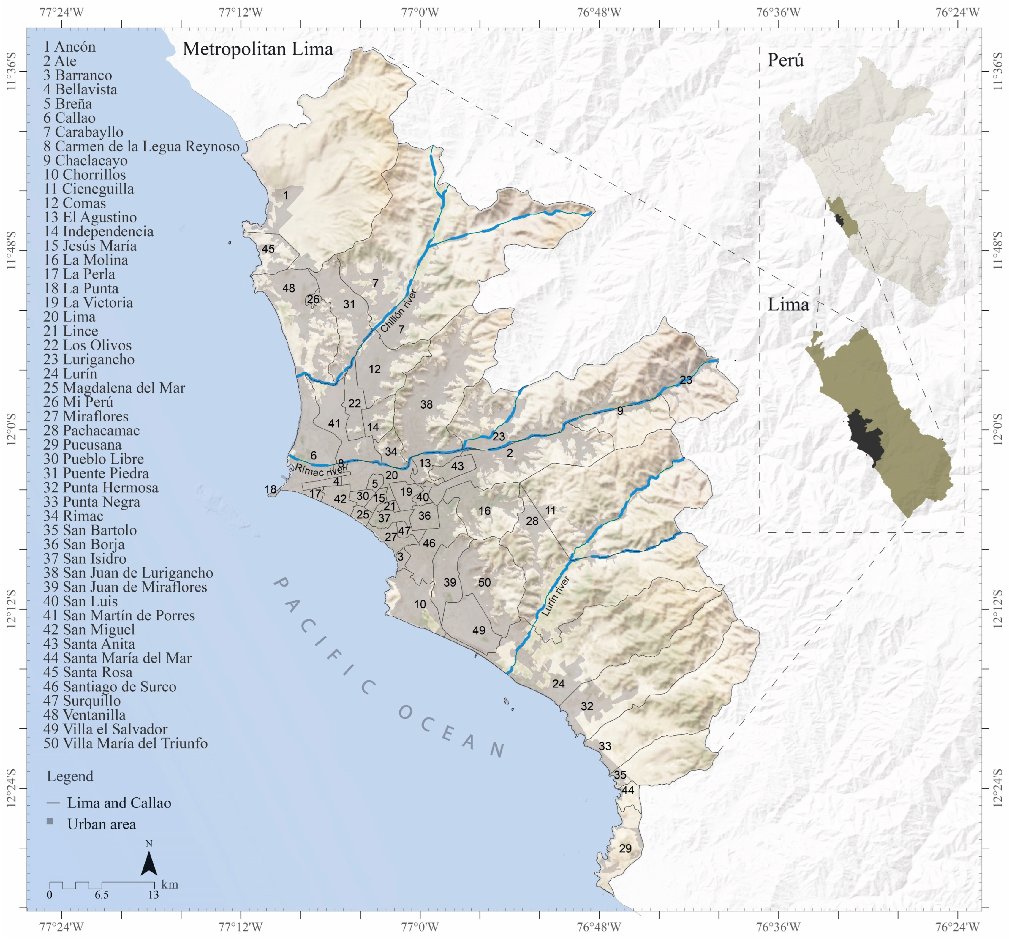
2.1. Study Area

The metropolitan city of Lima, the capital of Peru, consists of the urban area of the districts in Lima and the Constitutional Province of Callao. Located on the country’s central coast, its geographical position is approximately 12°5′00″S latitude and 77°2′00″W longitude. This mega city has a unique environmental setting, bordered to the west by the waters of the Pacific Ocean and to the east by the foothills of the Andes Mountains, which extend toward the valleys of the Rímac, Chillón, and Lurín rivers [32] (see Figure 1). Lima covers an area of 2840.35 km², with its urban area occupying approximately 32.5% of its total surface. The city’s elevation varies between 22 and 1179 m.a.s.l. Lima’s climate is warm and arid throughout the year, with maximum temperatures ranging from 19 °C in the south to 31 °C in the north. Annual precipitation is less than 15 mm, with high air humidity saturation, leading to the presence of drizzle or “garúa” in the winter (from June to August) [33]. Additionally, Lima plays a crucial role as the country’s main socioeconomic center, concentrating around 45% of Peru’s GDP and being fundamental in import and export activities [34].

2.2. Source of Spatial Data

2.2.1. Information Source for Urban Area Delimitation

The administrative–territorial delimitation at the provincial and district levels nationwide was obtained from the official website of the National Geographic Institute (IGN) of Peru, available at: https://www.idep.gob.pe/geovisor/df2 (accessed 25 May 2024), the competent authority in cartography in the country. From this, the district vector layers of the Constitutional Province of Callao and districts of the Province of Lima were selected and separated to cover the entire urban area of Metropolitan Lima. The updated vector layers of the urban boundaries of the districts in the Province of Lima were acquired through a formal request to the Metropolitan Municipality of Lima, addressed to the Urban Development Management through the Sub-management of Planning and Urban Enabling. For the Constitutional Province of Callao, the delimitation of the urban area was manually generated through a detailed verification of high-resolution images from the updated Google Satellite base map, available in QGIS software version 3.34.9.

2.2.2. Land Surface Temperature (LST)

The approach proposed by Ermida et al. [35] was used to obtain LST. It was obtained by applying the statistical mono-window (SMW) algorithm, based on a simple linear regression between the brightness temperature at the top of the atmosphere (TOA) captured in the thermal infrared (TIR) channel and LST. This model simplifies the radiative transfer equation while maintaining a direct relationship with surface emissivity. The implementation used a JavaScript code that is available at: https://earthengine.googlesource.com/users/sofiaermida/landsat_smw_lst (accessed 2 June 2024) on the Google Earth Engine (GEE) platform [36].

For the calibration of the Landsat series, surface reflectance data from each mission were used, available in GEE, and provided by the United States Geological Survey (USGS). Each Landsat sensor requires specific calibration due to differences in their spectral response functions, which can be consulted at the following link: https://code.earthengine.google.com/?accept_repo=users/sofiaermida/landsat_smw_lst (accessed 2 June 2024). However, the calibration coefficients are generally similar among the different sensors and consistently reflect the thermal infrared (TIR) bands.

The radiometric calibration was carried out using brightness temperatures at the top of the atmosphere (TOA), derived from the raw orthorectified digital numbers through the calibration coefficients provided by the USGS [37]. This procedure ensures the consistency and inter-calibration of the Landsat series. Cloud cover information, including shadows, was obtained from the quality assessment band (BQA) and is also available through the USGS in GEE. Preprocessing included resampling all TIR bands to a spatial resolution of 30 m, which is essential for maintaining consistency in the datasets used for analysis. This approach ensures accuracy in data comparison across different Landsat missions, thus enhancing the robustness of the LST trend analysis results [38].

The USGS provides the surface reflectance (SR) data from each Landsat sensor, which is available in GEE. In the case of Landsat 8, the SR is obtained through the LaSRC algorithm (Landsat Surface Reflectance Code), which applies an atmospheric correction based on a radiative transfer model, using atmospheric auxiliary data from MODIS and the coastal aerosol band to evaluate aerosol inversion [39]. For the Landsat 5 sensors, the SR is calculated using the LEDAPS algorithm (Landsat Ecosystem Disturbance Adaptive Processing System), which employs radiative transfer models with atmospheric data from MODIS and NCEP (National Centers for Environmental Prediction) [35].

Image mosaics were generated, and the median of pixels was obtained during the summer months, from January to April, between 1986 and 2024. Winter data were not included due to the high presence of cloud cover along the Peruvian coast [25]. These data are available for the Landsat 4, 5, 7, and 8 satellites; however, only Landsat 5 and 8 images were used in this study. Additionally, Landsat 7 was avoided due to banding issues in the images, so 2003 and 2012 were excluded from the LST analysis. Similarly, the Landsat 5 images from 2003 were excluded due to the lack of quality images (cloud-free) during the evaluated month period.

2.2.3. Fractional Vegetation Cover (FVC)

The FVC index was used to analyze vegetation covers in urban green areas. This index directly represents the fraction of the surface covered by vegetation, expressed as a percentage, facilitating its interpretation. Additionally, it offers greater accuracy in heterogeneous areas, such as urban zones, and is more stable against atmospheric variations or high aerosol levels. Another significant advantage is that it tends to saturate less in areas with high vegetation density. This index is generated from the normalized difference vegetation index (NDVI) [40,41], considering values greater than 0.15 for this study to expand the range of temporal analysis and capture vegetation changes. The details of the equation to obtain FVC are described below:

$$FVC={\displaystyle \frac{NDVI-{NDVI}_{min}}{{NDVI}_{max}-{NDVI}_{min}}}$$

(1)

where ${NDVI}_{min}$ corresponds to the NDVI of the soil in the total absence of vegetation and ${NDVI}_{veg}$ represents an area entirely covered by vegetation.

To ensure that vegetation is being analyzed, only values from an FVC of 0.25 were considered [42,43], meaning that only pixels with at least 25% vegetation were considered. This ensured that areas with high vegetation density, which could affect LST, were being analyzed.

Before analysis, the FVC datasets for the years considered were organized into an image collection list to normalize the data, ensuring that the FVC values from different sensors were comparable. This exact procedure was applied to analyze LST data within the GEE platform.

2.3. Mann–Kendall Trend Analysis

The trend evaluation of LST and FVC was conducted over the entire time series (1986–2024) for each pixel using the non-parametric Mann–Kendall (MK) test [43]. This test, known for its low sensitivity to outliers, is based on data ranking. Various studies have validated its effectiveness [44,45]. Through this method, it was possible to identify positive or negative trends, and through additional statistical analyses, the significance level was determined, as described in the following section. The analysis was implemented using a JavaScript script developed in the Google Earth Engine (GEE) platform, following the approach proposed by Foushee [46]. The equation is calculated as follows:

$$MK=\sum _{i=1}^{n-1}\sum _{j=i+1}^{n}sign\left(x_i-x_j\right)$$

(2)

where n is the number of data points and xi and xj are values in the time series at points i and j, where j > i. The sign function sign(xi − xj) is dependent on the sign and is interpreted as follows:

$$sign\left(x_i-x_j\right)=\left\{\begin{array}{c}+1if{x}_i-x_j>0\\ 0if{x}_i-x_j=0\\ -1if{x}_i-x_j<0\end{array}\right.$$

(3)

The variance is calculated as follows:

$$VAR\left(MK\right)={\displaystyle \frac{n\left(n-1\right)\left(2n-5\right)-{\sum }_{i=1}^m{t}_i(t_i-1)(2t_i+5)}{18}}$$

(4)

where n represents the time series length, m is the number of tied groups, and tᵢ denotes the number of ties of length i. This is used to assess data dispersion.

The calculated values serve as the input for computing the Z-score to evaluate significance as follows:

$$Z=\left\{\begin{array}{c}{\displaystyle \frac{MK-1}{\sqrt{VAR\left(MK\right)}}},ifMK>0\\ 0,ifMK=0\\ {\displaystyle \frac{MK+1}{\sqrt{VAR\left(MK\right)}}},ifMK<0\end{array}\right.$$

(5)

A positive or negative Z score indicates an increasing or decreasing trend, respectively, while a Z score of 0 indicates no trend. The comparison between Z and the standard normal variable at the desired significance level α allows for testing the trend’s significance. This procedure was implemented in Google Earth Engine using the code available at the following link: https://developers.google.com/earth-engine/tutorials/community/nonparametric-trends (accessed 3 June 2024).

The operation results can be classified into nine categories (see

Table 1. Trend classification criteria according to statistical significance.

MK Value Range	Z Value Range	p-Value	Category
$S>0$	$Z>2.58$	<0.001	Positive trend highly significant
	$1.96<Z\le 2.58$	<0.01	Positive trend significant
	$1.65<Z\le 1.96$	<0.05	Positive trend little significant
	$Z\le 1.65$	<0.1	Non-significant trend
$S=0$	$Z=0$	>0.1	No change
$S<0$	$Z\le 1.65$	<0.1	Non-significant trend
	$1.65<Z\le 1.96$	<0.05	Negative trend little significant
	$1.96<Z\le 2.58$	<0.01	Negative trend significant
	$Z>2.58$	<0.001	Negative trend highly significant

) [44]. All these analyses were finalized using QGIS software version 3.34.9.

2.4. Complementary Statistical Analyses

2.4.1. Correlation Analysis Between FVC and LST

A Spearman correlation analysis was performed per pixel, considering the evolution of FVC and LST from 1986 to 2024. The aim was to observe how an increase or decrease in FVC influenced the mitigation of LST variation. This analysis is a non-parametric correlation measure suitable for ordinal-scale data. It does not assume a normal distribution or any predefined relationship between the data [45]. The equation used is as follows:

$$r_s=1-{\displaystyle \frac{6\sum d_i^2}{n(n^2-1)}}$$

(6)

$$d_i=rg\left(X_i\right)-rg\left(Y_i\right)$$

(7)

where $r_s$ is Spearman’s rho or Spearman’s correlation coefficient; rg(Xi) and rg(Yi) are the ranks of each observation in samples X and Y; and n is the number of observations per pixel between 1986 and 2024 for both FVC and LST. This coefficient can range from −1 to 1, where −1 indicates a perfect negative correlation, 1 indicates a perfect positive correlation, and 0 indicates no correlation.

To calculate the significance level of the Spearman correlation coefficient, the following approximation was used since the sample size for each pixel is greater than 30 (n ≥ 30) [46]:

$$Z={\displaystyle \frac{r_s\sqrt{n-2}}{\sqrt{1-{r_s}^2}}}$$

(8)

where rₛ is the Spearman correlation coefficient and n is the total number of observations. The significance analysis was performed similarly to the trend analysis according to the Z values detailed in Table 1. This analysis was conducted in R Studio using the raster and dplyr packages in version 4.3.3 [47,48].

2.4.2. Multivariate Analysis

A hierarchical cluster analysis was performed on the mean temporal data of FVC and LST, with intervals of 5 to 6 years, considering data clarity, to group districts with similar characteristics. To achieve this, data were normalized before applying the clustering algorithm. The Ward method was also used, and a centroid-based classification with Euclidean distance was adopted.

To identify, classify, and categorize the districts according to the degree of LST variation mitigation due to green areas through FVC, a PCA (principal component analysis) was conducted to reduce the dimensionality of 8 variables from 50 districts while retaining essential data information. The considered variables included the mean trend of FVC and LST, the number of pixels comprising the green area, the proportion of green area per district, two variables representing average FVC in 1986 and 2024, and two variables representing average LST in 1986 and 2024. The three components that explained 80.20% of data variability were selected from these. These three components were subsequently used to perform the hierarchical cluster analysis using the Ward method, based on the Euclidean distance centroid. All these analyses were conducted using InfoStat version 2020 statistical software [49].

3. Results

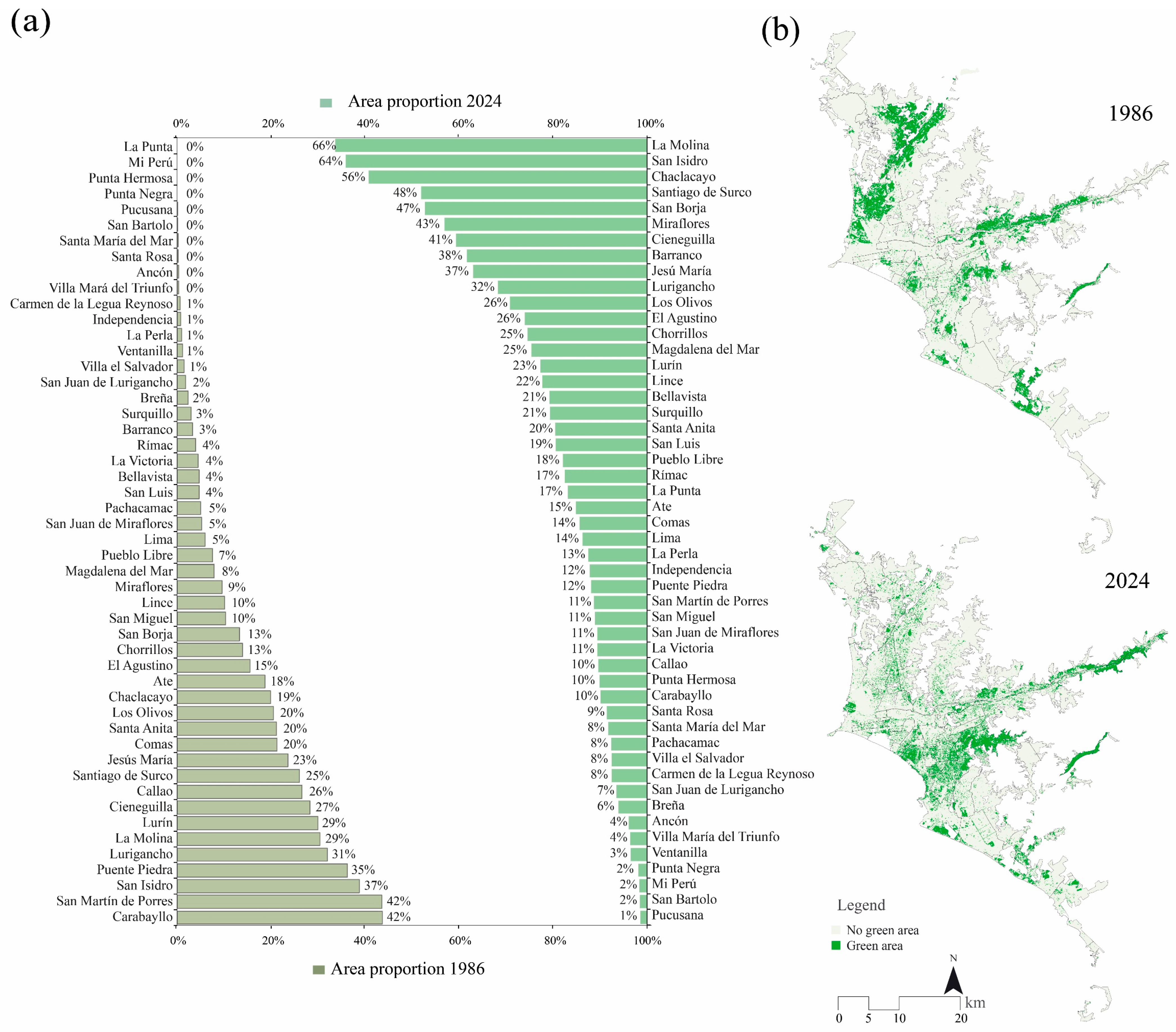
3.1. Proportion of Green Areas by Districts

An initial overview of the performance, transition, and translocation of green areas in Metropolitan Lima can be observed in Figure 2. In this initial assessment, it is evident that some districts have adequately managed their green areas, while others have not prioritized their development, instead installing impermeable materials such as concrete.

The districts that have increased their proportion of green areas by 2024 are La Molina, from 29% in 1986 to 66% in 2024; San Isidro, from 37% to 64%, doubling its proportion; Chaclacayo, from 19% to 59%; and Santiago de Surco, from 25% to 48%. These districts have climbed positions by investing in increasing green areas, mainly located in the central–southeastern part of the city (see Figure 2a,b). At the same time, these districts—La Molina, San Isidro, Surco, San Borja, and Miraflores—coincidentally host the population with the wealthiest level in Lima. Similarly, San Borja, which increased from 13% (1986) to 47% (2024), and Miraflores, which grew from 9% (1986) to 43% (2024), are the districts with the most significant increase in area compared to the previous ones, reaching up to five times their proportion of vegetation cover.

On the other hand, a drastic change is observed in the districts that, in 1986, had large expanses of green areas and, by 2024, show a significant decrease in their vegetation cover. Carabayllo has gone from having 42% green areas to only 10%; San Martín de Porres has fallen from 42% to 11%; and Puente Piedra has reduced its proportion from 35% to 12% (see Figure 2a). These districts, located mainly in the far north of the city (Figure 2b), had the highest percentage of green areas in 1986, including agricultural land. However, they have undergone substantial changes in land use due to urbanization, transforming what were once spaces with abundant vegetation into small, isolated patches without interconnection. Nonetheless, although the areas with more vegetation are highlighted, it is necessary to mention that a large part of the city lacks green areas, and many of them have remained so over the years, with few or insignificant modifications. These districts are mainly distributed in the city’s central, southern, and northern parts, such as Ventanilla, Villa María del Triunfo, Villa El Salvador, Breña, and La Victoria (see Figure 2b).

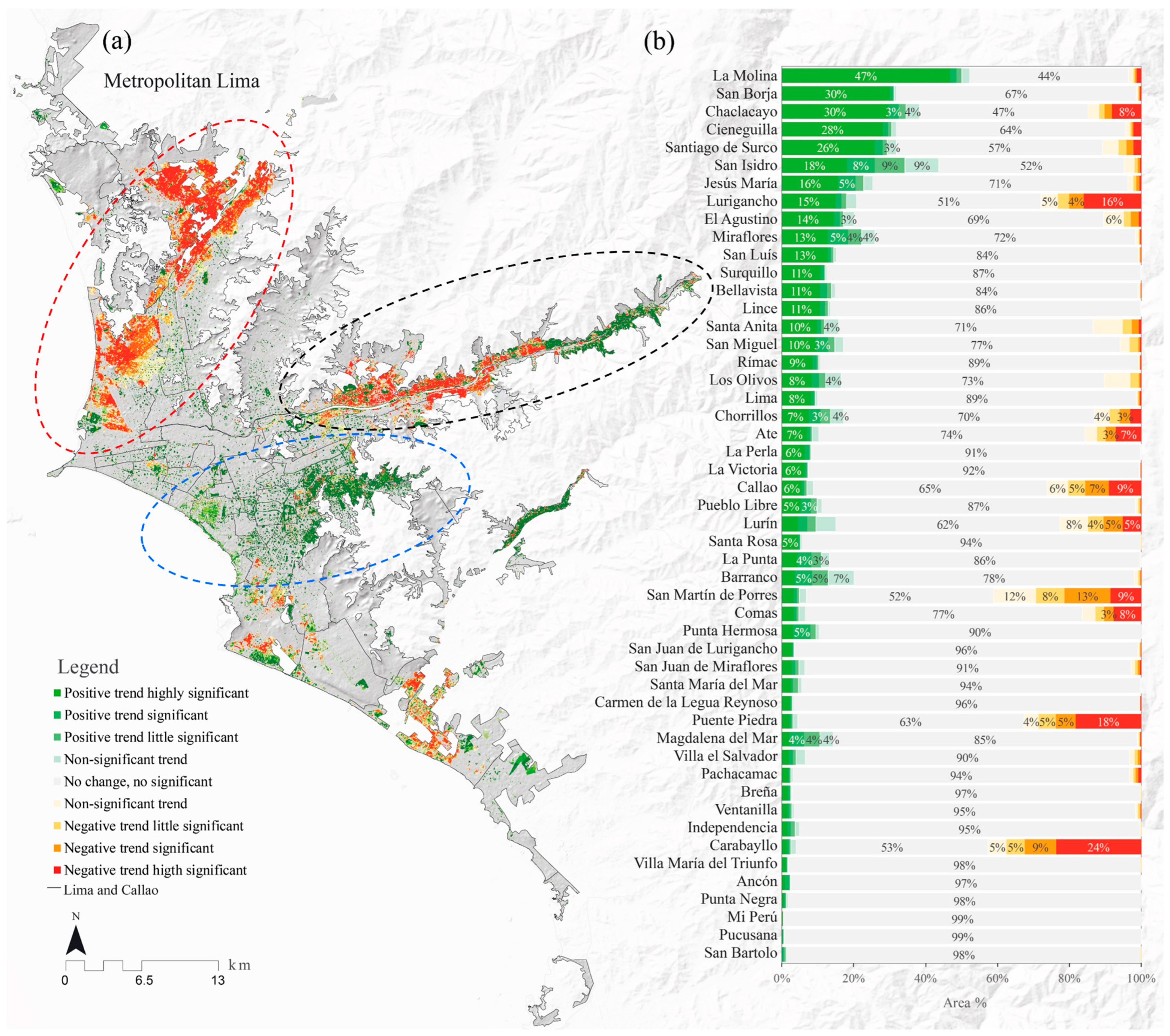
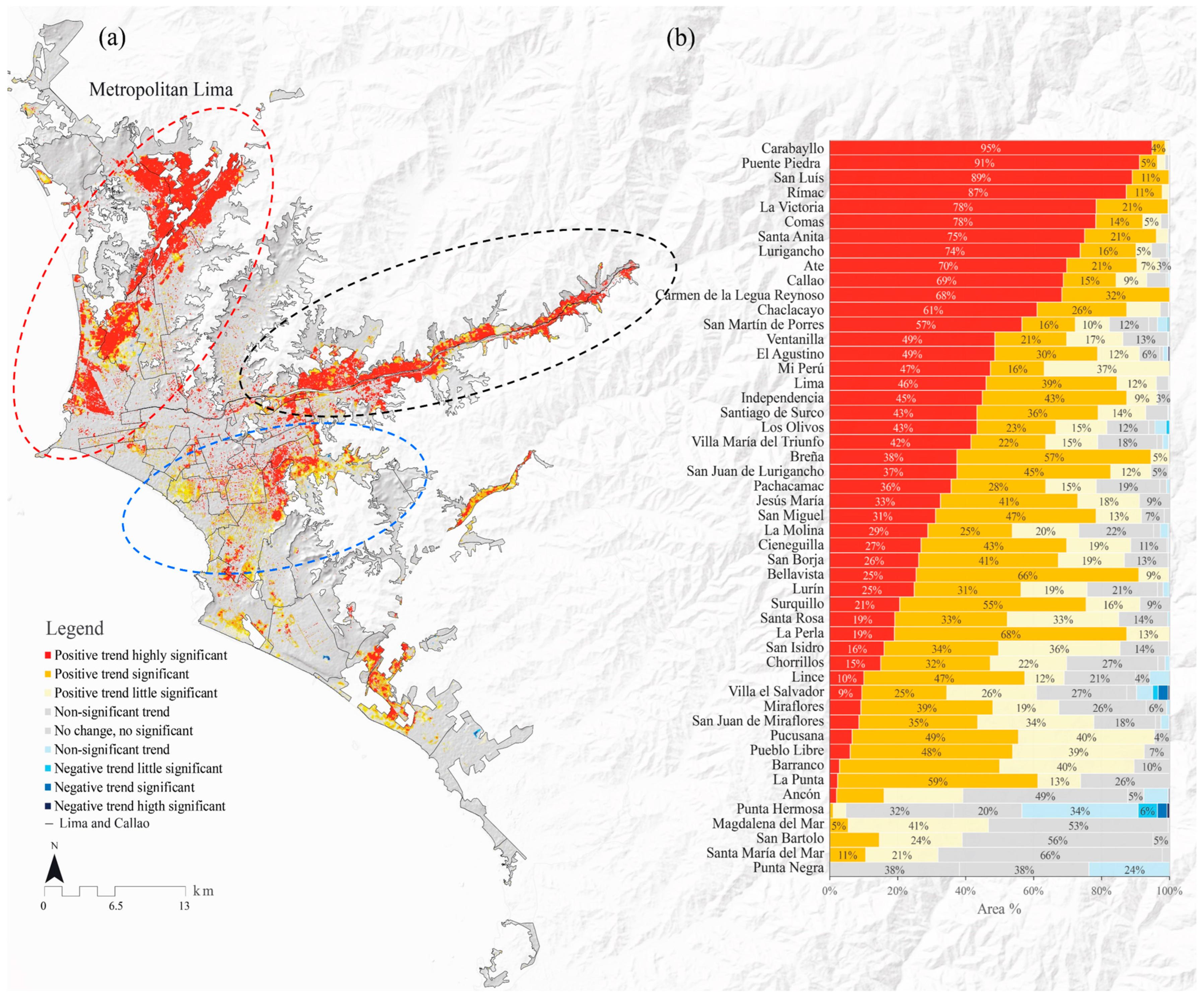
3.2. Trend Results of FVC and LST

The trend results of FVC are shown in Figure 3. An analysis of the area proportion according to the nine Mann–Kendall trend categories described in Table 1 is provided (Figure 3a). Information is given on the proportion of green areas that have been implemented (positive trend; p < 0.001) or degraded (negative trend; p < 0.001) in each district.

The districts with the highest proportion of implemented green spaces are located in the center and the southeastern and eastern strip, where the districts of La Molina (47%), San Borja (30%) (blue line), Chaclacayo (30%), and Cieneguilla (28%) are found (Figure 3b). These districts have a high socioeconomic population and are generally known for showing proper and planned urban management. On the other hand, the districts that present vegetation degradation in green areas are found in the north, central north, and east, in emerging peripheral districts, such as Carabayllo (24%), Lurigancho—Chosica (16%), San Martín de Porres (9%), and Comas (8%), among others (red and black lines, Figure 3b). Contrary to the other districts, these are related to medium and low socioeconomic strata (Figure 3b). Additionally, it should be considered that these are young peripheral districts that have developed informally without proper planning. The spaces occupied correspond mainly to agricultural use areas and often to spaces with steep slopes (hillsides).

The places that have not experienced significant green area development are also identified, meaning those that have not shown relevant changes (represented in gray on the map in Figure 3). It is interpreted that the proportion of vegetation is very low in these spaces, where there are no green areas and where their presence remains minimal. This situation is observed in various parts of the city, which are urban spaces where the implementation of green areas is not being prioritized despite their importance for the population’s well-being.

Figure 4 shows the LST trend in the green areas of Metropolitan Lima. Significant positive trends (p < 0.01) and highly significant positive trends (p < 0.001) are observed in almost all green areas of the districts. This suggests that, despite the development of urban vegetation, its impact on LST reduction is limited over time. The most pronounced trends are found in the peripheral districts, where there has been a considerable loss of vegetation (Figure 4b). Among these, Carabayllo stands out, with 95% of a highly significant positive trend (p < 0.001); Puente Piedra, with 91%; San Luis, with 89%; Rímac, with 87%; and Comas and La Victoria, with 78% each (see Figure 4a). These green spaces, with evident vegetation degradation, are mainly located in the north (dashed red line) and east (dashed black line) of the city and are primarily composed of agricultural land and abundant vegetation in a developing urban environment (see Figure 4b).

On the other hand, the districts that have increased their green area mostly present significant positive LST trends (p < 0.01), although some show slightly insignificant negative trends (p < 0.05). This is the case of La Molina, Miraflores, San Isidro, and San Borja (dashed blue lines). In these districts, slight negative trends are observed in spaces where the effects of water bodies and vegetation combine, significantly enhancing LST reduction. This effect is notable in districts such as La Molina, Villa El Salvador, Punta Hermosa, and Lurín, although it is associated with industrial-use water infrastructure in the latter two.

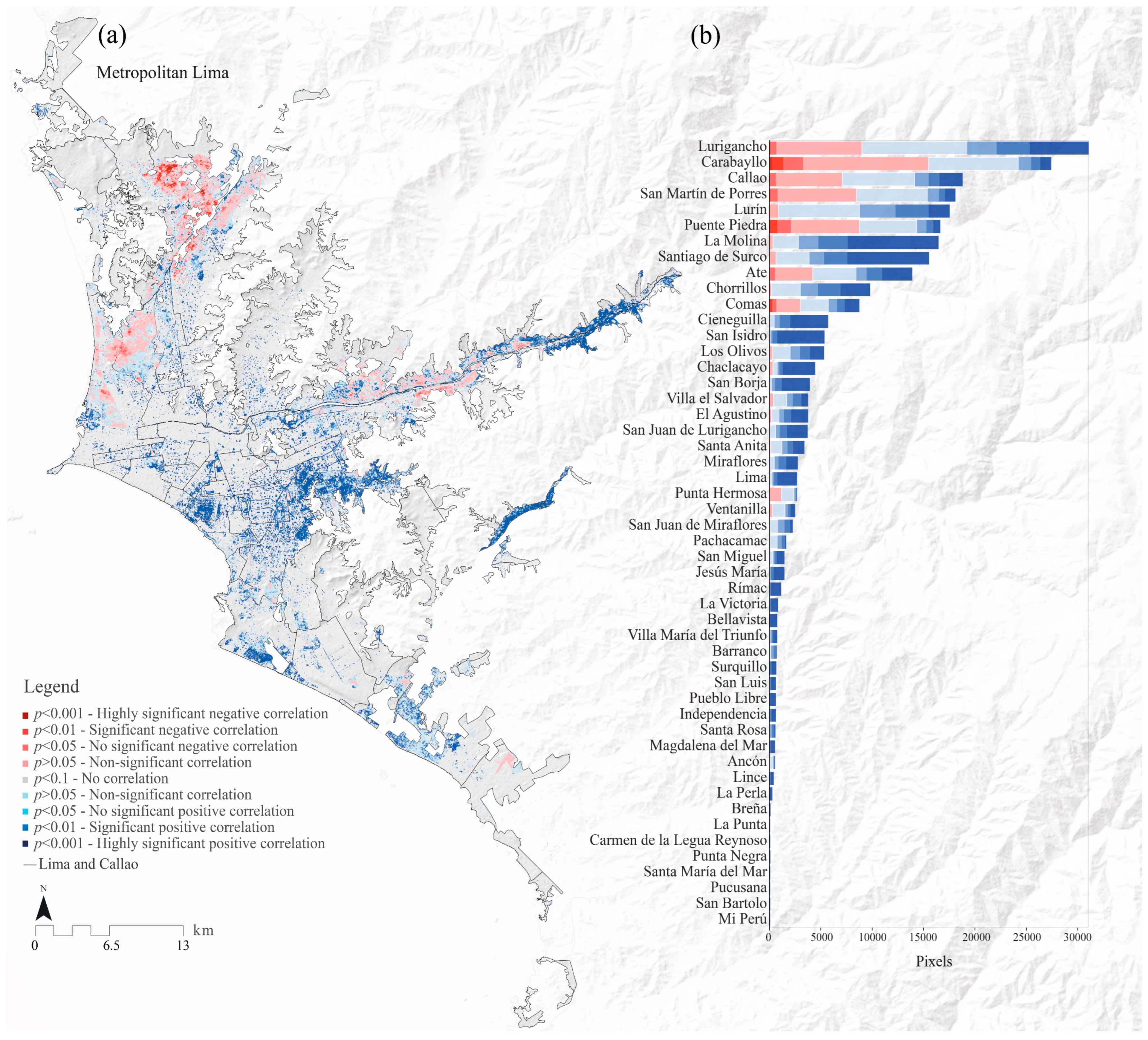
3.3. Trend Relationship Between FVC and LST

The average trend of each district was calculated using zonal statistics, and a Cartesian graph divided into four quadrants was generated to analyze the relationship between the trends of FVC and LST (Figure 5). A negative trend is observed in the data dispersion (Figure 5) when examining the overall relationship. However, most districts have a positive trend line (blue circle) in the first quadrant. This implies that, despite the increase in vegetation, there is also an increase in LST, which is unusual since a higher FVC is generally expected to be associated with a lower LST.

Districts such as La Molina and San Borja have also significantly contributed to creating green infrastructure. Nevertheless, despite these efforts, the overall trend has not significantly reduced LST, at least when considering its impact over the evaluation period.

In the fourth quadrant, the districts that have experienced a considerable loss of vegetation during the evaluated period are located, showing a negative trend in FVC and a positive trend in LST (red line). This is consistent, given that the absence of vegetation contributes to an increase in LST. A particular case is the district of Punta Hermosa, where the effect of FVC shows a significantly higher mitigation power in reducing LST compared to the other districts. This phenomenon may be attributed to the proximity of water bodies, such as the sea, and industrial-purpose water infrastructure, which favorably impacts nearby green spaces.

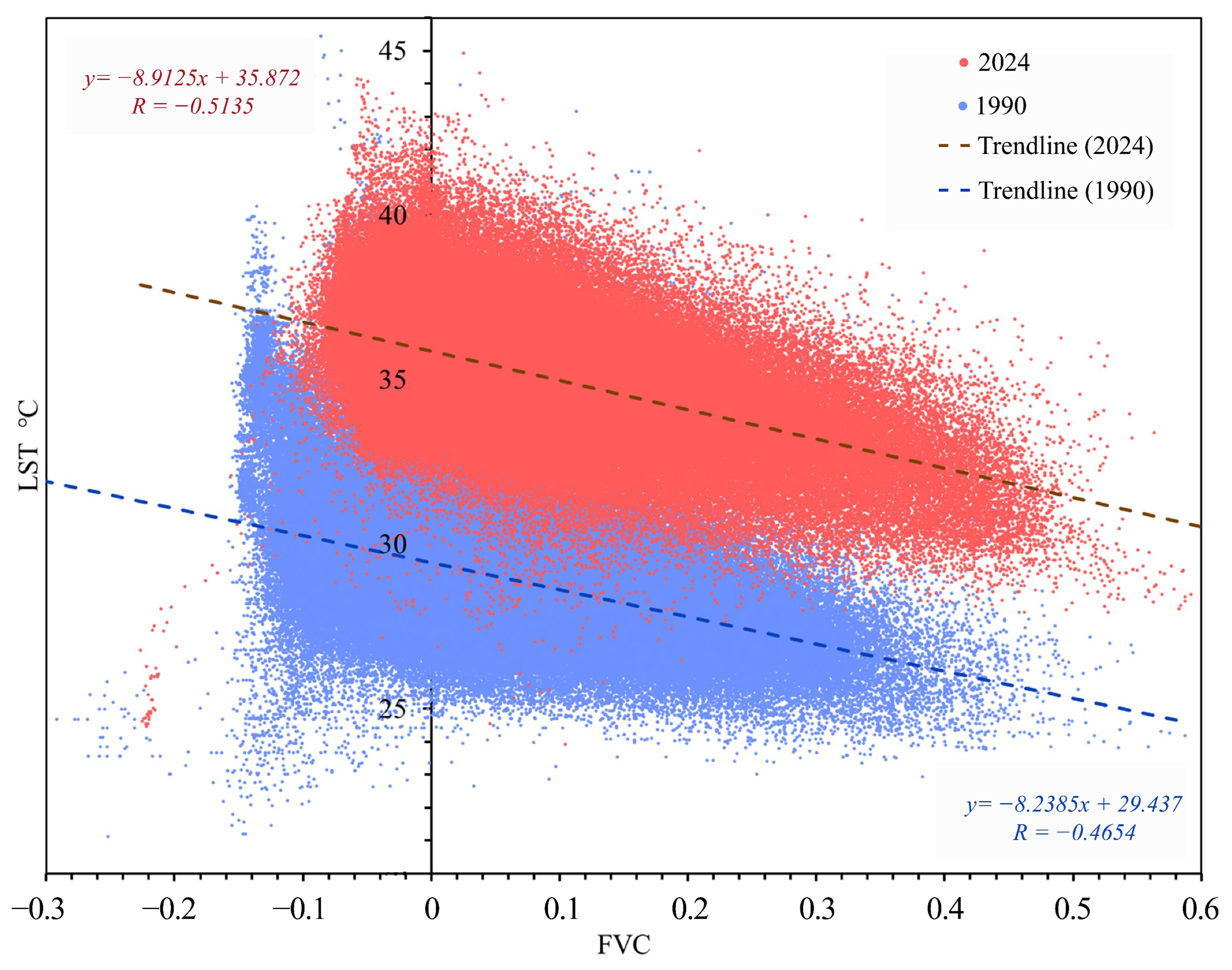
3.4. Spearman Relationship Between FVC and LST for the Period 1986–2024

Figure 6 shows the Spearman correlation between FVC and LST from the 1986–2024 period. This analysis, conducted on a pixel-by-pixel basis, evaluates how these two variables behave over time. It is observed that, in some districts, such as La Molina, Santiago de Surco, San Borja, and San Isidro, there is a highly significant positive correlation between FVC and LST in much of their territory (p < 0.001) where green areas are present (Figure 6b). This indicates that these areas experience an increase in both FVC and LST. However, some areas within these districts do not correlate significantly. These cases are related to the reduction in LST due to the presence of water bodies and the considerable increase in FVC, which are associated with factors such as the shade generated by tall buildings, contributing to lowering LST.

On the other hand, districts with a significant negative correlation (p < 0.05) can be observed, especially in areas where vegetation loss has occurred, leading to a reduction in FVC. Examples of these districts include Lurigancho (Chosica), Carabayllo, Callao, Ate, Puente Piedra, and San Martín de Porres (Figure 6a), where the increase in LST is exacerbated by horizontal urbanization, often with little or no urban planning, and other land-use changes that replace vegetation.

When analyzing the relationship between FVC and LST within the same year, it is observed that vegetation fulfills its mitigating function in LST variation (Figure 7): the higher the FVC, the lower the LST. However, notable differences in LST values are evident when comparing correlations between different years, such as 1990 and 2024. The increase in LST is undeniable, with an average variation of 6.43 °C from 1990 to 2024. This means that LST increased by 21.86% over this period. These findings corroborate previous results, where an apparent increase in LST is observed.

Meanwhile, the FVC shows that vegetation adapts to these changing conditions and continues to play its mitigating role, as a higher proportion of FVC results in a lower LST. It is important to note that, spatially, vegetation effectively mitigates LST fluctuations (Figure 7). However, at the temporal level, the analysis reveals a significant increase in LST (Figure 4). At the same time, vegetation has adapted to this gradual increase in LST over the evaluation period, maintaining low LST levels in areas with higher FVC.

To provide a broader overview of how the mean FVC and LST variables have changed over the evaluated period, Figure 8 is presented. Through a cluster analysis, grouping districts that exhibit similar behaviors was possible. Specific years that provided greater clarity in spatial data were prioritized.

Regarding LST evolution, a considerable increase is observed in all districts, although in different magnitudes. Districts experiencing an early rise in LST can be identified as located in the clusters of the green and red boxes, while the rest show a more moderate increase, as observed in the clusters of the blue boxes. Conversely, some districts have maintained low LST levels, with slight variation, as shown in the cyan and violet boxes (Figure 8a).

On the other hand, the evaluation of FVC in Figure 8b reveals noticeable differences among the districts. Some start with low levels and end with high levels of FVC (red and green boxes), while others begin with high levels and conclude with low levels (blue boxes). Unlike the others, stability in FVC levels is observed in the green box, with slight variation over time. Additionally, districts in the violet box show the most sustained and uniform increase in FVC over time, suggesting a clear trend toward prioritizing the establishment of green areas.

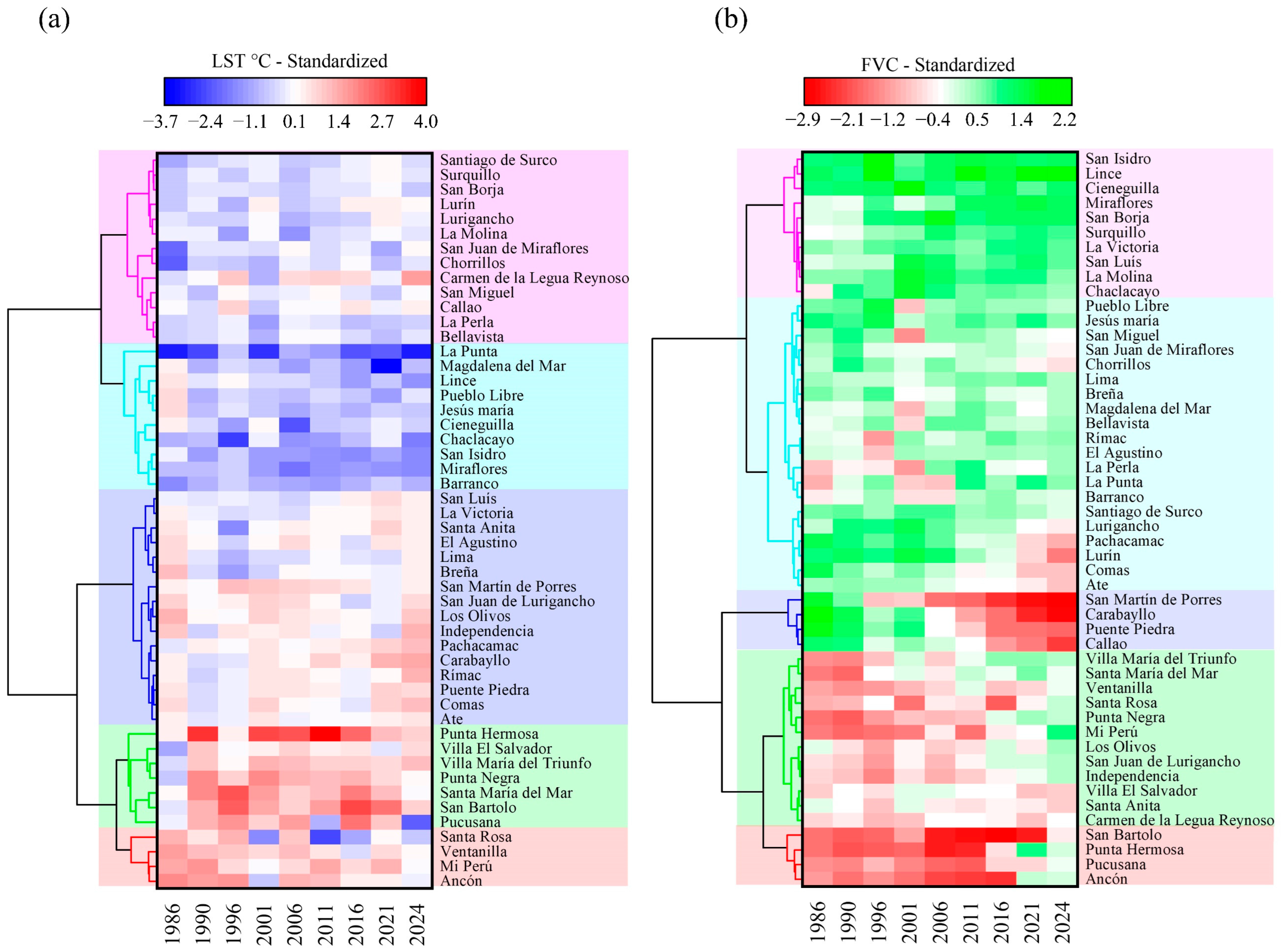
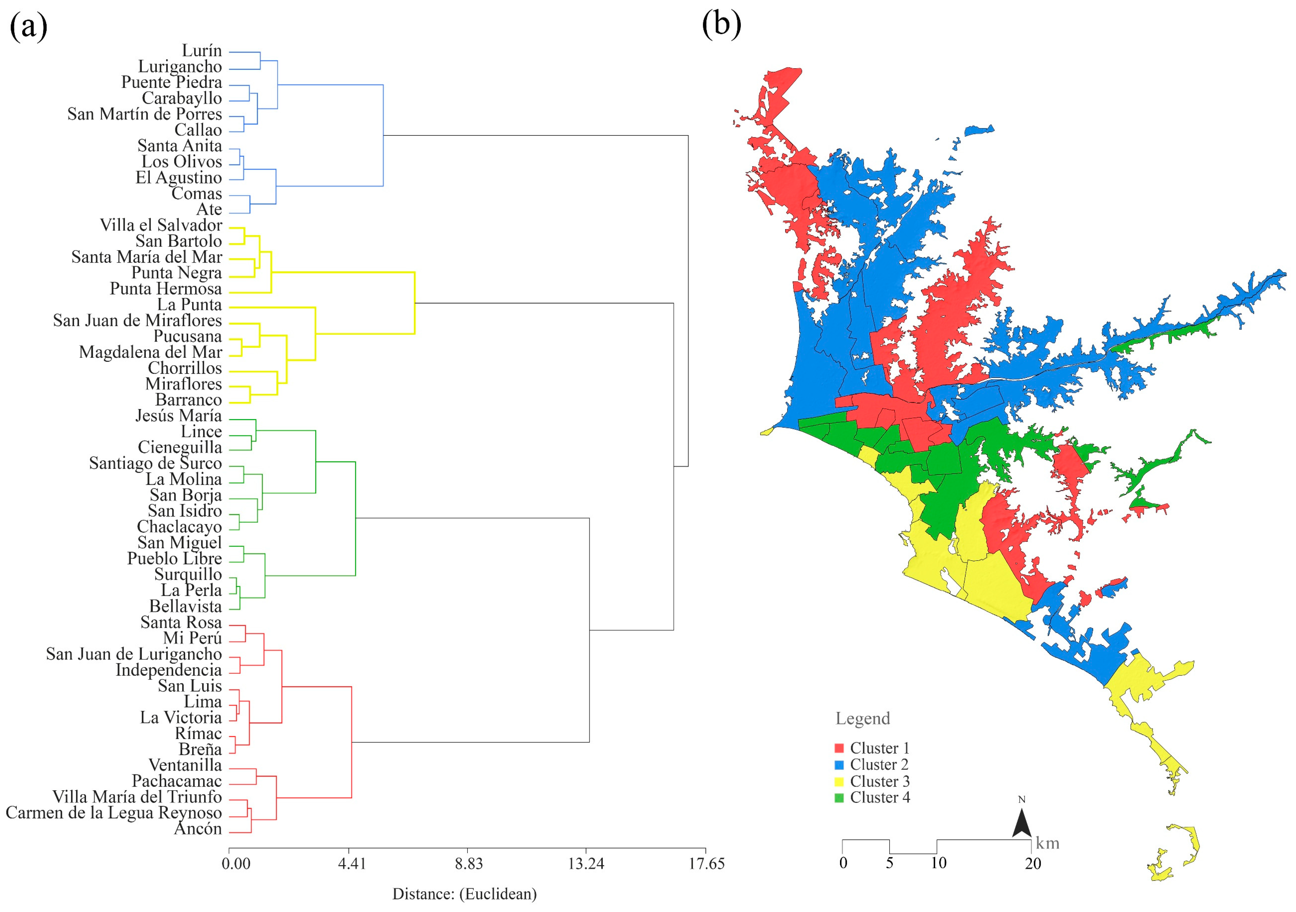
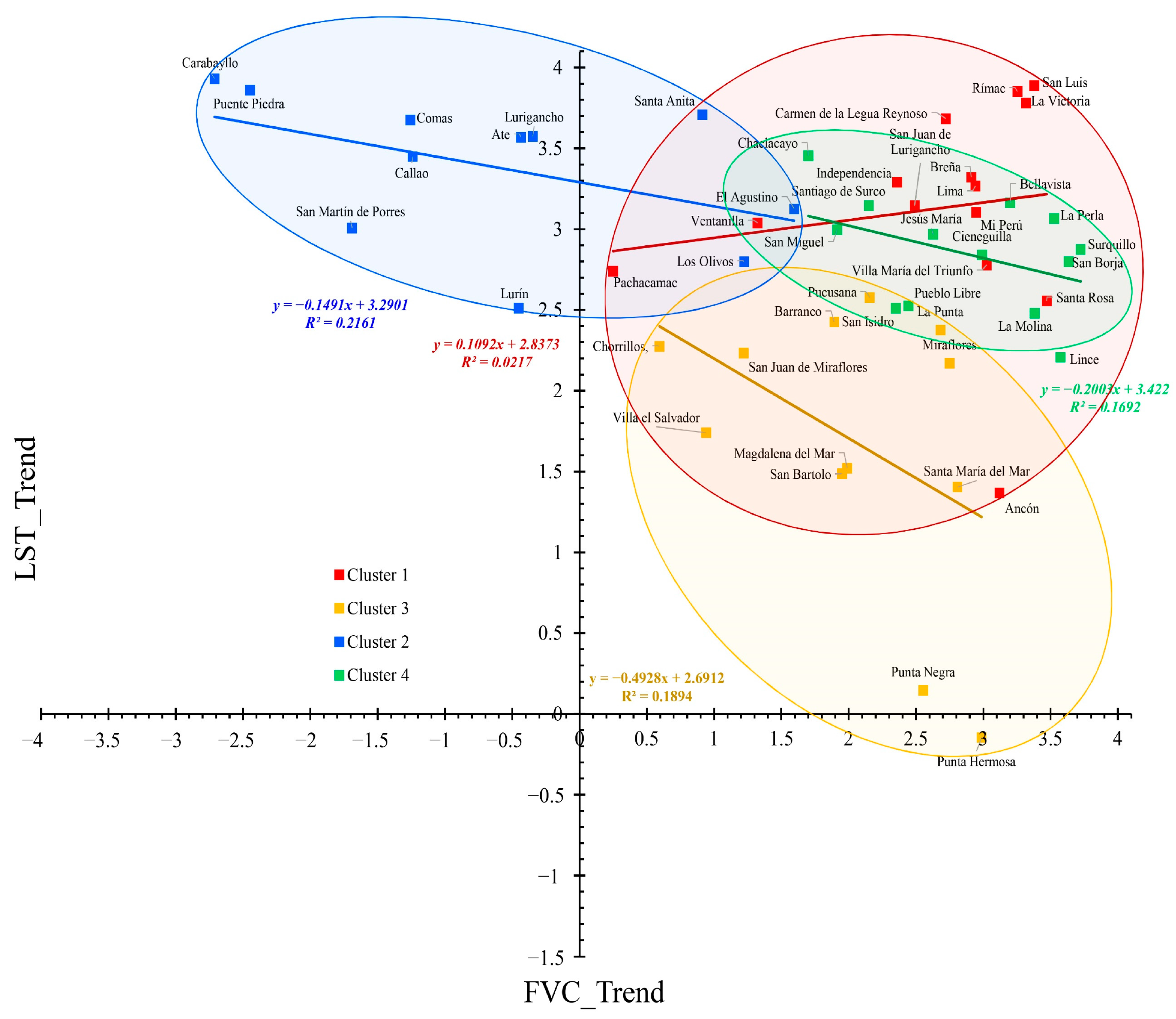
3.5. Identification, Categorization, and Classification of Districts Based on Trend Characteristics and Correlation of FVC and LST

After displaying and analyzing the trends and relationship between FVC and LST in green areas, a principal component analysis (PCA) was conducted to reduce data dimensionality. Three principal components were selected, explaining 80.20% of the total variability, with significant influence from four variables: average FVC trend, average LST trend, green area size, and the average FVC value for 2024. This allowed for a cluster analysis, enabling the classification and categorization of districts (Figure 9).

Four district clusters were identified, each with specific characteristics detailed in

Table 2. Classification and categorization characteristics of district clusters based on trend and spatial correlation analysis of FVC and LST.

Indicators	Cluster 1	Cluster 2	Cluster 3	Cluster 4
FVC Trend	Highly significant positive	Highly significant negative	Significant negative	Highly significant positive
LST Trend	Highly significant positive	Highly significant positive	Significant positive	Significant positive
Correlation	Highly significant positive	Significant negative	Non-significant negative	Highly significant positive
Area	Small	Large	Small	Large
Interconnection	No interconnection	With interconnection	No interconnection	With interconnection
FVC–LST Trend Relationship Line	Non-significant positive	Significant negative	Non-significant negative	Non-significant negative
Adjustment Model and R2	y = 0.1092x + 2.8373 R2 = 0.0217 (p > 0.05)	y = −0.1491x + 3.2901 R2 = 0.2161 (p < 0.05)	y = −0.4928x + 2.6912 R2 = 0.1894 (p > 0.05)	y = −0.2003x + 3.422 R2 = 0.1692 (p > 0.05)
Number of Districts	14	11	12	13
Performance	Acceptable	Deficient	Deficient	Excellent

.

• Cluster 1: This cluster comprises 14 districts with small, recently created green patches with limited spatial connectivity (lacking biological corridors). Additionally, these districts exhibit extensive horizontal urban development. This cluster shows a highly significant positive trend in FVC (p < 0.001) and LST (p < 0.001), indicating a highly significant positive correlation as well (p < 0.001).
• Cluster 2: Includes 11 districts, the largest in area, located in the city’s peripheral zones. It shows a highly significant positive trend in LST (p < 0.001) and a highly significant negative trend in FVC (p < 0.001) attributed to vegetation loss. Moreover, it presents a weakly significant negative correlation (p < 0.05). These districts had extensive agricultural areas at the beginning of the evaluation period.
• Cluster 3: Comprises 12 districts with unique behavior, displaying a significant positive trend in LST (p < 0.05) and a weakly significant negative trend in FVC (p < 0.05). The mitigation of LST changes could be attributed to sea breeze effects due to proximity to the ocean and artificial water bodies created for industrial purposes. The correlation is low in this case, showing a non-significant positive correlation (p > 0.05).
• Cluster 4: Includes 13 districts with a significant positive trend in LST (p < 0.05) and a highly significant positive trend in FVC (p < 0.001). These districts contain larger green areas that have consistently increased throughout the evaluation period. They are notable for their commitment to green space implementation and exhibit high interconnectivity, including the presence of biological corridors, considering their spatially interconnected configuration.

After performing multivariate analyses and classifying green areas in Metropolitan Lima, a new analysis of the relationship between FVC and LST trends was conducted. This analysis considers the identified clusters, as detailed in Figure 10 and Table 2, to observe how district grouping changes compared to Figure 5.

Unlike the previous analysis shown in Figure 5, Figure 10 highlights significant differences due to the influence of several additional factors mentioned in Section 2.4.2, simplifying the relationship between FVC and LST. In this case, all relationships exhibit a negative trend, a classic correlation between FVC and LST, except for Cluster 1, which shows a positive trend. This predominant negative relationship is expected between FVC and LST, though it is essential to consider that the time factor has been incorporated through the trend. Considering this, it is understandable to observe positive relationships, as in the case of Cluster 1, due to the increase in FVC and LST in these districts.

Figure 10 maintains the expected negative relationship: higher FVC corresponds to lower LST. For example, although Clusters 1 and 4 presents high LST levels, the mitigating effect of FVC is evident in these districts.

In contrast, Cluster 3 exhibits a variable mitigating effect; despite having small green spaces, it presents the lowest LST levels, possibly influenced by other climatic and local infrastructure factors. On the other hand, Cluster 2 stands out for its high LST levels and low FVC levels, indicating the absence or degradation of vegetation and, therefore, a lack of a mitigating effect.

4. Discussion

The dynamics of green areas in Metropolitan Lima reflect a complex interaction between urban development, the management of these spaces, and the decisions of social actors. According to this study, these dynamics are key to mitigating the increase in LST, a rising phenomenon (Figure 4 and Figure 7). By analyzing green area trends spatially and temporally through FVC, it is observed that some districts have prioritized their expansion, while others have experienced significant reductions due to urban growth. These differences are attributed to the unequal socioeconomic development of the 2000s, which drove investments in infrastructure but also accentuated social segmentation and disparities in the distribution and quality of green spaces [50]. Higher-income sectors tend to have greater access to parks and ecosystem services, improving their quality of life [51]. At the same time, lower-income districts face barriers to accessing these spaces [52], exacerbating social inequity and reducing quality of life [53].

The urbanization model in Lima sees public spaces and green areas as ornamental rather than recreational or as a means to improve quality of life, a common trend in Latin America [54]. This limits access to those who can afford it [55], as evidenced by the strong relationship between green areas and real estate prices, which explains 80.20% of price variability [56]. Their value is based on aesthetic rather than functional criteria, making them symbols of social distinction. However, the population does not perceive the scarcity of quality public green spaces as a problem; instead, they adapt and survive in precarious conditions, losing their sense of belonging as citizens of Lima [57]. This trend reflects how unplanned urban expansion and development with residential/commercial/industrial infrastructures exacerbate inequalities in access to public resources, including green spaces [58]. The lack of strategic urban planning that prioritizes equitable access to green areas has further entrenched these disparities, unconsciously promoting urban environmental injustice [59]. The absence of strategic planning prioritizes economic growth over green areas [60], perpetuating a cycle of inequality that deprives marginalized communities of benefits such as improved mental health and community cohesion [61].

This research shows a significant increase in LST in Metropolitan Lima between 1986 and 2024, with local reductions in areas with a higher proportion of vegetation. This trend is due to the proliferation of impermeable surfaces, such as asphalt and concrete, which retain more heat than vegetation [10]. Replacing green areas with buildings and roads reduces the natural cooling effects provided by vegetation, which generally moderates LST through processes like evapotranspiration [62]. Additionally, increased population density and vehicular traffic contribute to higher heat emissions and pollutants, further intensifying the urban heat island effect [63]. This phenomenon is accentuated in warm climates such as the Peruvian coast, exacerbating the impacts of climate change [64]. It is important to consider that Lima is located in an arid and warm desert ecosystem, making it constantly exposed to extreme temperature increases. In this context, green areas play a crucial role in mitigating the impact of urban climate warming. These effects are causing an increase in ambient temperatures, worsening urbanization effects, and increasing water demand [65]. As the climate warms, the frequency and intensity of heat waves will likely increase, presenting additional challenges for cities like Lima, which already deal with high LST [25,66].

A study by Amaya et al. [67] indicates that Lima’s urban area, situated in an arid and desert ecosystem, has a lower LST than the natural desert surroundings. This would explain why the city’s peripheral areas present high LST values due to higher albedo, radiation, and irradiation inherent to the predominant material in desert ecosystems. Likewise, LST differences could also be influenced by the predominant type of urban expansion. High LST values are observed in areas with horizontal urban expansion, mainly in new and peripheral zones with scarce green areas and a predominance of informal, vulnerable, and self-built constructions without proper planning [68]. In contrast, vertical urban expansion, which presents lower LST values, is characterized by tall buildings that generate shade, larger green areas, fully paved streets with asphalt or concrete, and locations near the sea. This type of expansion is also typically better planned and regulated, with stricter adherence to basic technical standards established by local governments [69].

This study also demonstrates that green areas effectively mitigate LST fluctuations by analyzing the spatial correlation between FVC and LST in independent years. This behavior aligns with numerous studies that highlight the benefits of green areas on LST. For example, it has been reported that urban green spaces can reduce LST by up to 5 °C compared to other types of urban land cover, with a notable cooling effect of approximately 4 °C observed with just a 10% increase in green cover in residential areas [3]. Similarly, Bao et al. [70] found that larger and more regularly shaped green areas exhibited greater cooling distances, suggesting that vegetation’s quantity and spatial arrangement play a vital role in mitigating urban heat. This would explain why mitigation is more efficient in areas with a higher proportion of green spaces, such as La Molina, San Borja, and San Isidro, compared to places where green patches exist without interconnections, such as Los Olivos, San Juan de Lurigancho, and San Martín de Porres (Figure 2). Additionally, the potential influence of nearby water bodies should not be underestimated, as they significantly help reduce LST, as seen in La Molina and San Borja, which have artificial water installations. Furthermore, the possibility of the influence of sea breezes from the ocean in districts such as Miraflores, Barranco, and San Borja should also be considered [71,72,73].

To improve the sustainability and management of green areas, it is essential to adopt successful experiences. Internationally, models such as Valencia’s Green Plan propose exceeding 11 m² of green area per inhabitant, integrating the protection and regeneration of natural heritage into urban planning [74]. Other proposals suggest that people should not live more than 300 m from a natural green area of at least 2 hectares, with a local nature reserve accessible for every 1000 inhabitants [75]. Curitiba has 52 m² of green area per person [76]. In Lima, some districts have successfully incorporated green areas into their urban fabric, offering valuable lessons for planning green infrastructures that integrate territorial and sectoral demands [77]. Likewise, protecting and restoring existing green spaces, such as hills and wetlands, are crucial to maintaining ecological networks that enhance urban connectivity and multifunctionality [78,79]. Integrating ecological considerations into urban development can mitigate adverse effects such as heat islands and provide ecosystem services, such as photosynthesis, ventilation, and recreation, improving urban resilience and mental well-being [80]. Effective governance and planning mechanisms are needed, especially in rapidly urbanizing contexts such as Lima [81].

Peru establishes regulations for public recreation areas (8–15%) and zonal parks (1–2%) depending on the type of urban development, whether for housing or urbanization, placing responsibility on municipalities for their proper distribution [82]. However, these regulations are not enforced for cultural and social reasons, leading to “gray cities.” To improve green area management, it is crucial to reevaluate service design in local governments, ensuring a more equitable distribution. This involves reclaiming and negotiating public space, strengthening local participation, and establishing a minimum cost per square meter in each district, guaranteeing adequate financing and oversight at the metropolitan level [83]. Additionally, it is essential to balance green area expansion with water consumption, a common challenge in cities with advanced vegetation development where water use for the population competes with that for green spaces [84,85]. This aspect is critical in Lima, a desert city with less than 50 mm of annual rainfall and the most populated city in Peru [33,86]. Selecting suitable vegetation is also essential, prioritizing native or introduced species with low water requirements that are adapted to arid climates and evaluating their functionality and utility in urban design [87,88]. Finally, it is important to consider the mountainous character of Lima’s large peripheral and vegetation-scarce districts, promoting solutions that consider the verticality of rural–urban linkages [89].

It is important to note that, considering the limitations of this research, the results presented are estimates and approximations of the impact of vegetation on LST. The pixel size used (30 m) in the images may, in some cases, not accurately reflect the local reality. However, at a macro level, it provides a general overview that allows for informed decision-making. Another aspect to consider is the lack of a deeper analysis that includes spatial, social, and economic factors of population behavior. These aspects could have been mentioned but are beyond the scope of this study, representing an area for future research. Another limitation is the classification and categorization of districts, which may be sensitive to including social and economic variables. Although these were not considered in this study, their incorporation would improve result accuracy. Despite these limitations, this study provides a preliminary view of green areas’ spatial distribution and temporal dynamics through FVC and LST. These findings could serve as valuable references for comparison with other cartographic representations in future studies, contributing to decision-making, urban management, and planning.

5. Conclusions

This study demonstrates that, between 1986 and 2024, the urban morphology of green areas in Metropolitan Lima has undergone significant changes in coverage, contributing, to some extent, to mitigating the increase in LST. Some districts, such as La Molina, San Isidro, Chaclacayo, Santiago de Surco, and San Borja, have significantly increased their proportion of green areas. In contrast, others, such as Carabayllo, San Martín de Porres, Puente Piedra, and Comas, have recorded significant vegetation losses. These changes have resulted in a general trend of increasing LST across the city, although this has been mitigated in areas with greater vegetation increases. A negative correlation between FVC and LST was observed in the spatial analysis of individual years, indicating that green areas contribute locally to reducing temperature. However, the temporal analysis shows a sustained increase in LST over time, suggesting that, although green areas are effective locally, they are insufficient to curb overall urban warming. This phenomenon is confirmed by the 21.86% increase in LST between 1990 and 2024.

Additionally, the cluster analysis identified four categories of districts, each with different levels of effectiveness in mitigating LST alteration, varying according to the extent and connectivity of their green areas. This classification reveals clear patterns among the different districts. Those with better planning and investment in green infrastructure show a notable performance in reducing LST. In contrast, districts with low vegetation cover and poor planning exhibit a marked increase in LST. This study underscores the importance of identifying, categorizing, and classifying districts based on the effectiveness of their green areas in reducing LST, providing a key perspective for addressing the challenges of urban growth. Future studies should include additional variables in their analyses, such as topography, evapotranspiration, proximity to bodies of water, and wind circulation, to better understand the factors affecting the relationship between FVC and LST. It is also essential to evaluate the ecosystem services provided by green areas, such as thermal comfort, and their impact on human well-being as well as socioeconomic factors and how the configuration of anthropogenic spaces influences the formation of urban heat islands. These considerations would improve the accuracy of evaluations and guide more effective adaptation and mitigation strategies.

The results obtained in this study highlight the need to strengthen policies for the management and expansion of green areas as a fundamental strategy for urban adaptation. This research provides valuable information for sustainable urban planning in Lima, emphasizing the crucial role of green areas in mitigating the effects of urban warming and enhancing the resilience and well-being of the city’s communities.

References

1. Bowler, D.E.; Buyung-Ali, L.; Knight, T.M.; Pullin, A.S. Urban greening to cool towns and cities: A systematic review of the empirical evidence. Landsc. Urban Plan. 2010, 97, 147–155. [Google Scholar] [CrossRef]
2. Blachowski, J.; Hajnrych, M. Assessing the Cooling Effect of Four Urban Parks of Different Sizes in a Temperate Continental Climate Zone: Wroclaw (Poland). Forests 2021, 12, 1136. [Google Scholar] [CrossRef]
3. Selim, S.; Eyileten, B.; Karakuş, N. Investigation of green space cooling potential on land surface temperature in Antalya city of Turkey. ISPRS—Int. Arch. Photogramm. Remote Sens. Spat. Inf. Sci. 2023, XLVIII-M-1, 107–114. [Google Scholar] [CrossRef]
4. Adulkongkaew, T.; Satapanajaru, T.; Charoenhirunyingyos, S.; Singhirunnusorn, W. Effect of land cover composition and building configuration on land surface temperature in an urban-sprawl city, case study in Bangkok Metropolitan Area, Thailand. Heliyon 2020, 6, e04485. [Google Scholar] [CrossRef] [PubMed]
5. Ahmed, B.; Kamruzzaman, M.; Zhu, X.; Rahman, M.S.; Choi, K. Simulating Land Cover Changes and Their Impacts on Land Surface Temperature in Dhaka, Bangladesh. Remote Sens. 2013, 5, 5969–5998. [Google Scholar] [CrossRef]
6. Zhang, M.; Tan, S.; Zhang, C.; Han, S.; Zou, S.; Chen, E. Assessing the impact of fractional vegetation cover on urban thermal environment: A case study of Hangzhou, China. Sustain. Cities Soc. 2023, 96, 104663. [Google Scholar] [CrossRef]
7. Arellano, B.; Roca, J. Effects of urban greenery on health. A study from remote sensing. Int. Arch. Photogramm. Remote Sens. Spat. Inf. Sci. 2022, XLIII-B3-2022, 17–24. [Google Scholar]
8. D’isidoro, M.; Mircea, M.; Borge, R.; Finardi, S.; de la Paz, D.; Briganti, G.; Russo, F.; Cremona, G.; Villani, M.G.; Adani, M.; et al. The Role of Vegetation on Urban Atmosphere of Three European Cities—Part 1: Evaluation of Vegetation Impact on Meteorological Conditions. Forests 2023, 14, 1235. [Google Scholar] [CrossRef]
9. Cai, Y.; Zhang, M.; Lin, H. Estimating the Urban Fractional Vegetation Cover Using an Object-Based Mixture Analysis Method and Sentinel-2 MSI Imagery. IEEE J. Sel. Top. Appl. Earth Obs. Remote Sens. 2020, 13, 341–350. [Google Scholar] [CrossRef]
10. Asi, A.N.H.; Supriatna, S.; Zulkarnain, F. Spatial Study of Land Cover Changes and Land Surface Temperature in Bekasi Regency, West Java, Indonesia. IOP Conf. Ser. Earth Environ. Sci. 2022, 1111, 012024. [Google Scholar]
11. Avdan, U.; Jovanovska, G. Algorithm for Automated Mapping of Land Surface Temperature Using LANDSAT 8 Satellite Data. J. Sens. 2016, 2016, 1480307. [Google Scholar] [CrossRef]
12. Sekertekin, A.; Zadbagher, E. Simulation of future land surface temperature distribution and evaluating surface urban heat island based on impervious surface area. Ecol. Indic. 2021, 122, 107230. [Google Scholar] [CrossRef]
13. Moisa, M.B.; Gabissa, B.T.; Hinkosa, L.B.; Dejene, I.N.; Gemeda, D.O. Analysis of Land Surface Temperature Using Geospatial Technologies in Gida Kiremu, Limu, and Amuru District, Western Ethiopia. Artif. Intell. Agric. 2022, 6, 90–99. [Google Scholar] [CrossRef]
14. Marufuzzaman, M.; Khanam, M.M.; Hasan, K. Monitoring the Land Cover Change and Its Impact on the Land Surface Temperature of Rajshahi City, Bangladesh using GIS and Remote Sensing Techniques. J. Geogr. Environ. Earth Sci. Int. 2021, 25, 1–19. [Google Scholar] [CrossRef]
15. Achmad, E.; Muryunika, R. Analysis of Vegetation Density and Land Surface Temperature Using Landsat Image in the Forest Area of KPHP Unit XII Batanghari. In Proceedings of the 3rd Green Development International Conference (GDIC 2020); Advances in Engineering Research. Atlantis Press: Dordrecht, The Netherlands, 2021; pp. 109–113. Available online: https://www.atlantis-press.com/proceedings/gdic-20/125960265 (accessed on 3 October 2024).
16. Phan, T.N.; Kappas, M.; Tran, T.P. Land Surface Temperature Variation Due to Changes in Elevation in Northwest Vietnam. Climate 2018, 6, 28. [Google Scholar] [CrossRef]
17. Zhao, L.; Lee, X.; Schultz, N.M. A wedge strategy for mitigation of urban warming in future climate scenarios. Atmos. Chem. Phys. 2017, 17, 9067–9080. [Google Scholar] [CrossRef]
18. Fan, X.; Tang, B.-H.; Wu, H.; Yan, G.; Li, Z.-L. A three-channel algorithm for retrieving night-time land surface temperature from MODIS data under thin cirrus clouds. Int. J. Remote Sens. 2015, 36, 4836–4863. [Google Scholar] [CrossRef]
19. Jiang, Y.; Fu, P.; Weng, Q. Assessing the Impacts of Urbanization-Associated Land Use/Cover Change on Land Surface Temperature and Surface Moisture: A Case Study in the Midwestern United States. Remote Sens. 2015, 7, 4880–4898. [Google Scholar] [CrossRef]
20. Sresto, M.A.; Siddika, S.; Fattah, M.A.; Morshed, S.R.; Morshed, M.M. A GIS and remote sensing approach for measuring summer-winter variation of land use and land cover indices and surface temperature in Dhaka district, Bangladesh. Heliyon 2022, 8, e10309. [Google Scholar]
21. INEI. Instituto Nacional de Estadistica e Informatica-Población de la Provincia de Lima Supera los 10 Millones 292 Mil Habitantes [Internet]. 2023. Available online: https://www.gob.pe/institucion/inei/noticias/894611-poblacion-de-la-provincia-de-lima-supera-los-10-millones-292-mil-habitantes (accessed on 4 October 2024).
22. INEI. Instituto Nacional de Estadistica e Informatica-Provincia Constitucional del Callao Alberga a Cerca de un Millón de Habitantes [Internet]. 2023. Available online: https://m.inei.gob.pe/prensa/noticias/provincia-constitucional-del-callao-alberga-a-cerca-de-un-millon-de-habitantes-7689/ (accessed on 4 October 2024).
23. World Population Review-Largest Cities by Population 2024 [Internet]. Available online: https://worldpopulationreview.com/cities (accessed on 4 October 2024).
24. Moya, L.; Vilela, M.; Jaimes, J.; Espinoza, B.; Pajuelo, J.; Tarque, N.; Santa-Cruz, S.; Vega-Centeno, P.; Yamazaki, F. Vulnerabilities and exposure of recent informal urban areas in Lima, Peru. Prog. Disaster Sci. 2024, 23, 100345. [Google Scholar] [CrossRef]
25. Cano, D.; Cacciuttolo, C.; Haller, A.; Rosario, C.; Guerra, J.C.; de Oliveira, G.G. Spatio-temporal tendencies of urban land surface temperature on the Andean piedmont under climate change: A case study of Metropolitan Lima, Peru (1986–2024). Remote Sens. Appl. Soc. Environ. 2024, 36, 101378. [Google Scholar] [CrossRef]
26. Ascencio, E.J.; Barja, A.; Benmarhnia, T.; Carrasco-Escobar, G. Disproportionate exposure to surface-urban heat islands across vulnerable populations in Lima city, Peru. Environ. Res. Lett. 2023, 18, 074001. [Google Scholar] [CrossRef]
27. Limache, C.T. Quantification of the benefits derived from the Nature Based Solutions in the very arid and densified urban context of metropolitan Lima. Rev. LABVERDE 2022, 12, 207–243. [Google Scholar] [CrossRef]
28. Inostroza, L.; Csaplovics, E. Measuring Climate Change Adaptation in Latin-America. Spatial Indexes for Exposure, Sensitivity and Adaptive Capacity to Urban Heat Islands in Lima and Santiago de Chile; Lincoln Institute of Land Policy Working Paper; Lincoln Institute of Land Policy: Cambridge, CA, USA, 2014; 103p. [Google Scholar]
29. Siña, M.; Wood, R.C.; Saldarriaga, E.; Lawler, J.; Zunt, J.; Garcia, P.; Cárcamo, C. Understanding Perceptions of Climate Change, Priorities, and Decision-Making among Municipalities in Lima, Peru to Better Inform Adaptation and Mitigation Planning. PLoS ONE 2016, 11, e0147201. [Google Scholar] [CrossRef]
30. Cárdenas-Mamani, Ú.; Perrotti, D. An integrated urban metabolism and ecosystem service assessment: The case study of Lima, Peru. J. Ind. Ecol. 2024, 28, 1567–1581. [Google Scholar] [CrossRef]
31. Moreno, R.; Nery, A.; Zamora, R.; Lora, Á.; Galán, C. Contribution of urban trees to carbon sequestration and reduction of air pollutants in Lima, Peru. Ecosyst. Serv. 2024, 67, 101618. [Google Scholar] [CrossRef]
32. Facchini, A.; Mele, R.; Caldarelli, G. The Urban Metabolism of Lima: Perspectives and Policy Indications for GHG Emission Reductions. Front. Sustain. Cities 2021, 2, 40. [Google Scholar] [CrossRef]
33. SENAMHI. Servicio Nacional de Meteorología e Hidrología del Perú-Lima Registró Lluvia de Moderada Intensidad [Internet]. 2020. Available online: https://www.senamhi.gob.pe/?p=prensa&n=1129 (accessed on 4 October 2024).
34. APEC. Partnerships for the Sustainable Development of Cities in the APEC Region [Internet]. Cities Alliance. 2018. Available online: https://www.citiesalliance.org/resources/publications/cities-alliance-knowledge/partnerships-sustainable-development-cities-apec (accessed on 4 October 2024).
35. Ermida, S.L.; Soares, P.; Mantas, V.; Göttsche, F.-M.; Trigo, I.F. Google Earth Engine Open-Source Code for Land Surface Temperature Estimation from the Landsat Series. Remote Sens. 2020, 12, 1471. [Google Scholar] [CrossRef]
36. Gorelick, N.; Hancher, M.; Dixon, M.; Ilyushchenko, S.; Thau, D.; Moore, R. Google Earth Engine: Planetary-scale geospatial analysis for everyone. Remote Sens. Environ. 2017, 202, 18–27. [Google Scholar] [CrossRef]
37. Good, E.J.; Aldred, F.M.; Ghent, D.J.; Veal, K.L.; Jimenez, C. An Analysis of the Stability and Trends in the LST_cci Land Surface Temperature Datasets Over Europe. Earth Space Sci. 2022, 9, e2022EA002317. [Google Scholar] [CrossRef]
38. Wang, M.; Zhang, Z.; He, G.; Wang, G.; Long, T.; Peng, Y. An enhanced single-channel algorithm for retrieving land surface temperature from Landsat series data. J. Geophys. Res. Atmos. 2016, 121, 11712–11722. [Google Scholar] [CrossRef]
39. Vermote, E.; Justice, C.; Claverie, M.; Franch, B. Preliminary Analysis of the Performance of the Landsat 8/OLI Land Surface Reflectance Product. Remote Sens. Environ. 2016, 185, 46–56. [Google Scholar] [CrossRef] [PubMed]
40. Carlson, T.N.; Ripley, D.A. On the relation between NDVI, fractional vegetation cover, and leaf area index. Remote Sens. Environ. 1997, 62, 241–252. [Google Scholar] [CrossRef]
41. Orusa, T.; Viani, A.; Moyo, B.; Cammareri, D.; Borgogno-Mondino, E. Risk Assessment of Rising Temperatures Using Landsat 4–9 LST Time Series and Meta® Population Dataset: An Application in Aosta Valley, NW Italy. Remote Sens. 2023, 15, 2348. [Google Scholar] [CrossRef]
42. Qi, Y.; Li, H.; Pang, Z.; Gao, W.; Liu, C. A Case Study of the Relationship Between Vegetation Coverage and Urban Heat Island in a Coastal City by Applying Digital Twins. Front. Plant Sci. 2022, 13, 861768. [Google Scholar] [CrossRef]
43. Zhang, S.; Chen, H.; Fu, Y.; Niu, H.; Yang, Y.; Zhang, B. Fractional Vegetation Cover Estimation of Different Vegetation Types in the Qaidam Basin. Sustainability 2019, 11, 864. [Google Scholar] [CrossRef]
44. Cano, D.; Pizarro, S.; Cacciuttolo, C.; Peñaloza, R.; Yaranga, R.; Gandini, M.L. Study of Ecosystem Degradation Dynamics in the Peruvian Highlands: Landsat Time-Series Trend Analysis (1985–2022) with ARVI for Different Vegetation Cover Types. Sustainability 2023, 15, 15472. [Google Scholar] [CrossRef]
45. Hauke, J.; Kossowski, T. Comparison of values of Pearson’s and Spearman’s correlation coefficients on the same sets of data. Quaest. Geogr. 2011, 30, 87–93. [Google Scholar] [CrossRef]
46. Bonett, D.G.; Wright, T.A. Sample Size Requirements for Estimating Pearson, Kendall and Spearman Correlations. Psychometrika 2000, 65, 23–28. [Google Scholar] [CrossRef]
47. Hijmans, R.J.; Etten, J.v.; Sumner, M.; Cheng, J.; Baston, D.; Bevan, A.; Bivand, R.; Busetto, L.; Canty, M.; Fasoli, B.; et al. Raster: Geographic Data Analysis and Modeling [Internet]. 2024. Available online: https://cran.r-project.org/web/packages/raster/index.html (accessed on 25 October 2024).
48. Wickham, H.; François, R.; Henry, L.; Müller, K.; Vaughan, D.; Software, P. dplyr: A Grammar of Data Manipulation [Internet]. 2023. Available online: https://cran.r-project.org/web/packages/dplyr/index.html (accessed on 25 October 2024).
49. Di Rienzo, J.; Casanoves, F.; Balzarini, M.; Gonzalez, L.; Tablada, M.; Robledo, C. InfoStat Versión 2020; Universidad Nacional de Córdoba: Cordoba, Argentina, 2020; Available online: http://www.infostat.com.ar (accessed on 27 October 2024).
50. Fernández-de-Córdova, G.; Moschella, P.; Fernández-Maldonado, A.M. Changes in Spatial Inequality and Residential Segregation in Metropolitan Lima. In Urban Socio-Economic Segregation and Income Inequality; van Ham, M., Tammaru, T., Ubarevičienė, R., Janssen, H., Eds.; Springer: Cham, Switzerland, 2021. [Google Scholar] [CrossRef]
51. Nesbitt, L.; Meitner, M.J. Exploring Relationships between Socioeconomic Background and Urban Greenery in Portland, OR. Forests 2016, 7, 162. [Google Scholar] [CrossRef]
52. Dai, D. Racial/ethnic and socioeconomic disparities in urban green space accessibility: Where to intervene? Landsc. Urban Plan. 2011, 102, 234–244. [Google Scholar] [CrossRef]
53. Li, Y.; Svenning, J.-C.; Zhou, W.; Zhu, K.; Abrams, J.F.; Lenton, T.M.; Ripple, W.J.; Yu, Z.; Teng, S.N.; Dunn, R.R.; et al. Green spaces provide substantial but unequal urban cooling globally. Nat. Commun. 2024, 15, 7108. [Google Scholar] [CrossRef]
54. Bakhtsiyarava, M.; Moran, M.; Ju, Y.; Zhou, Y.; Rodriguez, D.A.; Dronova, I.; Pina, M.d.F.R.P.d.; de Matos, V.P.; Skaba, D.A. Potential drivers of urban green space availability in Latin American cities. Nat. Cities 2024, 1, 842–852. [Google Scholar] [CrossRef]
55. Vargas-Villafuerte, J.; Cuevas-Calderón, E.; Vargas-Villafuerte, J.; Cuevas-Calderón, E. Neoliberalización de la gestión urbana en Lima metropolitana, Perú. Rev. INVI 2022, 37, 71–97. [Google Scholar] [CrossRef]
56. Loret de Mola, U.; Ladd, B.; Duarte, S.; Borchard, N.; Anaya La Rosa, R.; Zutta, B. On the Use of Hedonic Price Indices to Understand Ecosystem Service Provision from Urban Green Space in Five Latin American Megacities. Forests 2017, 8, 478. [Google Scholar] [CrossRef]
57. Lafosse, P.V.C.S. La desigualdad invisible: El uso cotidiano de los espacios públicos en la Lima del siglo XXI. Territorios 2017, 36, 23–46. [Google Scholar]
58. Ploger, J. La formación de enclaves residenciales en Lima en el contexto de la inseguridad. Ur[B]Es 2007, 3, 14–20. [Google Scholar]
59. Romero, H.; Opazo, D. Ecología Política de los Espacios Urbanos Metropolitanos: Geografía de la Injusticia Ambiental. Geogr. J. Cent. Am. 2011, 2, 1–15. Available online: https://www.revistas.una.ac.cr/index.php/geografica/article/view/2470 (accessed on 28 October 2024).
60. Torres, S. One Metropolis, two scenarios. Sustainable Urban Development Contradictions in the Metropolitan Area of Lima. In Proceedings of the 56th ISOCARP World Planning Congress ‘Post-Oil City: Planning for Urban Green Deals’ Virtual Congress, Virtual, 8 November 2020–4 February 2021; p. 1512. Available online: https://isocarp.org/app/uploads/2021/06/ISOCARP_2020_Torres_44.pdf (accessed on 28 October 2024).
61. Liotta, C.; Kervinio, Y.; Levrel, H.; Tardieu, L. Planning for environmental justice—Reducing well-being inequalities through urban greening. Environ. Sci. Policy 2020, 112, 47–60. [Google Scholar] [CrossRef]
62. Li, D.; Bou-Zeid, E.; Oppenheimer, M. The effectiveness of cool and green roofs as urban heat island mitigation strategies. Environ. Res. Lett. 2014, 9, 055002. [Google Scholar] [CrossRef]
63. Nguyen, T.M.; Lin, T.-H.; Chan, H.-P. The Environmental Effects of Urban Development in Hanoi, Vietnam from Satellite and Meteorological Observations from 1999–2016. Sustainability 2019, 11, 1768. [Google Scholar] [CrossRef]
64. Giráldez, L.; Silva, Y.; Flores-Rojas, J.L.; Trasmonte, G. Diagnosis of the Extreme Climate Events of Temperature and Precipitation in Metropolitan Lima during 1965–2013. Climate 2022, 10, 112. [Google Scholar] [CrossRef]
65. Hommes, L.; Boelens, R. Urbanizing rural waters: Rural-urban water transfers and the reconfiguration of hydrosocial territories in Lima. Politi-Geogr. 2017, 57, 71–80. [Google Scholar] [CrossRef]
66. Tapia, V.L.; Vasquez-Apestegui, B.V.; Alcantara-Zapata, D.; Vu, B.; Steenland, K.; Gonzales, G.F. Association between maximum temperature and PM2.5 with pregnancy outcomes in Lima, Peru. Environ. Epidemiol. 2021, 5, e179. [Google Scholar] [PubMed]
67. Amaya, P.; Cuya, O.; Esenarro, D.; Vega, V.; Mendez, R. Green Infrastructure, Urban Heat Islands and Human Well—Being in the City of Metropolitan Lima; Haynes, R., Ed.; Pollution and Its Minimization; Springer Nature: Singapore, 2024; pp. 181–195. [Google Scholar]
68. Torres Obregón, D.; Perleche Ugás, D.; Aiquipa Zavala, A. Encuentros y desencuentros entre la planificación urbana y la realidad de la producción del espacio urbano en Lima metropolitana y el Callao (1961–2020). Rev. Geogr. Norte. Gd. 2022, 81, 35–54. [Google Scholar]
69. Noguerol Uceda, E. La Autonomía Municipal y el Desarrollo Urbano Sostenible en Lima Metropolitana. 2023. Available online: https://repositorio.ulima.edu.pe/handle/20.500.12724/19177 (accessed on 28 October 2024).
70. Bao, T.; Li, X.; Zhang, J.; Zhang, Y.; Tian, S. Assessing the Distribution of Urban Green Spaces and its Anisotropic Cooling Distance on Urban Heat Island Pattern in Baotou, China. ISPRS Int. J. Geo-Inf. 2016, 5, 12. [Google Scholar] [CrossRef]
71. Cai, Z.; Han, G.; Chen, M. Do water bodies play an important role in the relationship between urban form and land surface temperature? Sustain Cities Soc. 2018, 39, 487–498. [Google Scholar]
72. Louka, P.; Papanikolaou, I.; Petropoulos, G.P.; Kalogeropoulos, K.; Stathopoulos, N. Identifying Spatially Correlated Patterns between Surface Water and Frost Risk Using EO Data and Geospatial Indices. Water 2020, 12, 700. [Google Scholar] [CrossRef]
73. Wu, Z.; Zhang, Y. Water Bodies’ Cooling Effects on Urban Land Daytime Surface Temperature: Ecosystem Service Reducing Heat Island Effect. Sustainability 2019, 11, 787. [Google Scholar] [CrossRef]
74. Rojo, M.S.; Recasens, X. Espacios agroecológicos como soluciones basadas en la naturaleza para las infraestructuras verdes en España. Rev. Espanola Estud. Agrosociales Pesq. 2024, 263, 318–334. [Google Scholar] [CrossRef]
75. Pauleit, S.; Slinn, P.; Handley, J.; Lindley, S. Promoting the Natural Greenstructure of Towns and Cities: English Nature’s Accessible Natural Greenspace Standards Model. Built Environ. 2003, 29, 157–170. [Google Scholar] [CrossRef]
76. Fundación Mi Parque. La Gran Diferencia de m2 de Áreas Verde Por Persona en Latinoamérica—Fundación Mi Parque [Internet]. 2012. Available online: https://www.miparque.cl/es/la-gran-diferencia-de-m2-de-areas-verde-por-persona-en-latinoamerica/ (accessed on 28 October 2024).
77. Flores, O.M. Paisajes Resilientes. Reflexiones en torno a la reconstrucción de territorios desde el manejo y diseño de infraestructuras verdes, en el marco de las estrategias de gestión de riesgo ante desastres. Nadir Rev. Electrónica Geogr. Austral 2013, 5, 1–19. Available online: https://revistanadir.yolasite.com/a%C3%B1o-5-n-1-enero-julio-2013.php (accessed on 28 October 2024).
78. Jenerette, G.D.; Harlan, S.L.; Brazel, A.; Jones, N.; Larsen, L.; Stefanov, W.L. Regional relationships between surface temperature, vegetation, and human settlement in a rapidly urbanizing ecosystem. Landsc. Ecol. 2007, 22, 353–365. [Google Scholar] [CrossRef]
79. Reyes Päcke, S.; Figueroa Aldunce, I.M. Distribución, superficie y accesibilidad de las áreas verdes en Santiago de Chile. EURE 2010, 36, 89–110. [Google Scholar] [CrossRef]
80. Bosch, M.A.v.D.; Mudu, P.; Uscila, V.; Barrdahl, M.; Kulinkina, A.; Staatsen, B.; Swart, W.; Kruize, H.; Zurlyte, I.; Egorov, A.I. Development of an urban green space indicator and the public health rationale. Scand. J. Public Health 2015, 44, 159–167. [Google Scholar] [CrossRef] [PubMed]
81. Nieto, A.B.T.; Amezquita, J.L.N.; Vasquez, M.L. Governance of metropolitan areas for delivery of public services in Latin America. REGION 2018, 5, 49–73. [Google Scholar] [CrossRef]
82. Ministerio de Vivienda, Construcción y Saneamiento. Reglamento Nacional de Edificaciones-RNE [Internet]. 2021. Available online: https://www.gob.pe/institucion/vivienda/informes-publicaciones/2309793-reglamento-nacional-de-edificaciones-rne (accessed on 29 October 2024).
83. HacerPeru. La Desigualdad del Espacio Público en Lima: El Caso de los Parques y Jardines Públicos. [Internet]. 2017. Available online: http://hacerperu.pe/opiniones/la-desigualdad-del-espacio-publico-en-lima-el-caso-de-los-parques-y-jardines-publicos/ (accessed on 29 October 2024).
84. Gómez-Lobo, A.; Gutiérrez, M.; Huamaní, S.; Marino, D.; Serebrisky, T.; Solís, B. Access to water and COVID-19: A regression discontinuity analysis for the peri-urban areas of metropolitan Lima, Peru. Water Int. 2024, 49, 52–79. [Google Scholar] [CrossRef]
85. Ramirez Herrera, A.C.; Bauer, S.; Peña Guillen, V. Water-Sensitive Urban Plan for Lima Metropolitan Area (Peru) Based on Changes in the Urban Landscape from 1990 to 2021. Land 2022, 11, 2261. [Google Scholar] [CrossRef]
86. Metzger Terrazas, L.A. Análisis de Tendencias de Precipitación y Temperatura Considerando los Movimientos en Masa en el Departamento de Lima. Repos Inst-SENAMHI [Internet]. 2024. Available online: http://repositorio.senamhi.gob.pe/handle/20.500.12542/3258 (accessed on 29 October 2024).
87. Arhuire-Ossio, M.; Vélez-Azañero, A.; Quiros-Rossi, L.; Thomas, E.; Ladd, B. Optimizing water use efficiency in urban green space of a hyper-arid megacity through tree species selection: A case study. Urban Water J. 2022, 20, 1331–1335. [Google Scholar] [CrossRef]
88. Quispe Aguilar, E.B. Situación de las Áreas Verdes Urbanas en Lima Metropolitana. 2017. Available online: https://hdl.handle.net/20.500.12996/2990 (accessed on 29 October 2024).
89. Haller, A.; Branca, D. Urbanization and the Verticality of Rural–Urban Linkages in Mountains. In Montology Palimpsest: A Primer of Mountain Geographies; Sarmiento, F.O., Ed.; Springer International Publishing: Cham, Switzerland, 2022; pp. 133–148. [Google Scholar] [CrossRef]
Figure 1. Location map of the urban area of Metropolitan Lima and its districts. The assigned numbers correspond to the 50 districts ordered alphabetically, with boundary data from 2023.
Remotesensing 17 01323 g001
Figure 2. The proportion of green area by the district in 1986 and 2024 through the FVC index. (a) The horizontal bar chart on the left shows the proportion of green areas by district in 1986, and the right shows the proportion of green areas in 2024. (b) At the top is the spatial distribution of green areas in 1986, while at the bottom, 2024 is presented.
Remotesensing 17 01323 g002
Figure 3. Spatial analysis of the FVC trend based on the Mann–Kendall test. (a) Spatial distribution of FVC trends in the urban spaces of Metropolitan Lima. (b) The proportion of area covered by the district is classified according to statistical significance levels in FVC trends. The numbers accompanying the district names indicate their geographic location, as detailed in Figure 1.
Remotesensing 17 01323 g003
Figure 4. Spatial analysis of LST trends based on the Mann–Kendall test. (a) Spatial distribution of LST trends in the urban districts of Metropolitan Lima. (b) The proportion of area covered according to the level of statistical significance. The numbers preceding each district’s name correspond to their geographic location, as detailed in Figure 1.
Remotesensing 17 01323 g004
Figure 5. Relationship between FVC and LST trends. The first quadrant includes districts with positive trends in both indicators. The second quadrant comprises districts with negative FVC and positive LST trends. The third quadrant shows districts with negative trends in both indicators. Finally, the fourth quadrant contains districts with negative FVC and positive LST trends.
Remotesensing 17 01323 g005
Figure 6. Pixel-by-pixel Spearman correlation between FVC and LST for 1986–2024 in the urban districts of Metropolitan Lima. (a) Spatial distribution of the statistical significance level. (b) Number of pixels per district according to the statistical significance level.
Remotesensing 17 01323 g006
Figure 7. Correlation analysis of FVC and LST for the years 1990–2024.
Remotesensing 17 01323 g007
Figure 8. The average evolution of (a) LST and (b) FVC for each district during the 1986-2024 period, grouped according to cluster analysis. The units correspond to the standardized values of LST and FVC, respectively.
Remotesensing 17 01323 g008
Figure 9. Identification and classification of districts according to cluster analysis in mitigating LST variation. (a) Distribution of district classification and (b) spatial distribution of the groups resulting from the cluster analysis.
Remotesensing 17 01323 g009
Figure 10. Relationship analysis between FVC and LST trends considering classification after cluster analysis.
Remotesensing 17 01323 g010