Article

Interpretable Dual-Channel Convolutional Neural Networks for Lithology Identification Based on Multisource Remote Sensing Data

State Key Laboratory of Geological Process and Mineral Resources, Faculty of Earth Resources, China University of Geosciences, Wuhan 430074, China
*
Author to whom correspondence should be addressed.
Remote Sens. 2025, 17(7), 1314; https://doi.org/10.3390/rs17071314
Submission received: 25 February 2025 / Revised: 1 April 2025 / Accepted: 3 April 2025 / Published: 7 April 2025

Abstract

:
Lithology identification provides a crucial foundation for various geological tasks, such as mineral exploration and geological mapping. Traditionally, lithology identification requires geologists to interpret geological data collected from the field. However, the acquisition of geological data requires a substantial amount of time and becomes more challenging under harsh natural conditions. The development of remote sensing technology has effectively mitigated the limitations of traditional lithology identification. In this study, an interpretable dual-channel convolutional neural network (DC-CNN) with the Shapley additive explanations (SHAP) interpretability method is proposed for lithology identification; this approach combines the spectral and spatial features of the remote sensing data. The model adopts a parallel dual-channel structure to extract spectral and spatial features simultaneously, thus implementing lithology identification in remote sensing images. A case study from the Tuolugou mining area of East Kunlun (China) demonstrates the performance of the DC-CNN model in lithology identification on the basis of GF5B hyperspectral data and Landsat-8 multispectral data. The results show that the overall accuracy (OA) of the DC-CNN model is 93.51%, with an average accuracy (AA) of 89.77% and a kappa coefficient of 0.8988; these metrics exceed those of the traditional machine learning models (i.e., Random Forest and CNN), demonstrating its efficacy and potential utility in geological surveys. SHAP, as an interpretable method, was subsequently used to visualize the value and tendency of feature contribution. By utilizing SHAP feature-importance bar charts and SHAP force plots, the significance and direction of each feature’s contribution can be understood, which highlights the necessity and advantage of the new features introduced in the dataset.

Graphical Abstract

1. Introduction

Geological research is of great significance to human society, is closely related to socio-economic development, and has many benefits for all aspects of human production and life. Among these methods of research, lithology identification is a key aspect of geological survey work, and the resulting interpreted results are of great value in analyzing the geological conditions and mineralization potential of an area [1]. However, traditional methods of lithology identification face numerous challenges in complex geological settings, and the data collected require innovative approaches to improve lithological mapping accuracy and efficiency [2]. Remote sensing technology can instantiate a wide range of space-based observations on the ground without being limited by terrain, overcoming the limitations of the traditional methods [3,4]. Consequently, its application in the field of geological mapping has become increasingly widespread, particularly in lithology identification [5,6,7]. For example, Zhang Cuifen et al. [8] used WorldView-2 and ASTER multi-spectral data to extract remote sensing image information to practice lithology classification in the study area of West Kunlun. Liu et al. [9] successfully completed lithological classification in the Huangshan area of eastern Xinjiang by employing ASTER data with an Extreme Learning Machine (ELM) model.
In the data processing aspect of remote sensing technology, deep learning has been widely applied; deep learning is known for its hierarchical feature-extraction capabilities; the technology progressively combines lower-level features to create representations which are more abstract and complex. Therefore, deep learning has been proven to fully capture the hidden feature information in remote sensing data for lithology identification in recent studies [10,11,12,13]. Among the various deep learning models, convolutional neural networks (CNNs) have been widely used in lithology classification tasks because of their shared parameter-based characteristics and local receptive fields [14]. Imamverdiyev and Sukhostat (2019) introduced a 1D-CNN lithology identification model based on logging data and demonstrated that neural networks can significantly enhance lithology identification automatically [15]. Brandmeie and Chen (2019) utilized CNNs to identify olivine and carbonate sedimentary rocks on the basis of remote sensing images, confirming the effectiveness of CNNs [16]. Xu et al. (2021) proposed an intelligent lithology recognition method for rock images that was based on CNNs [17]. Li et al. (2022) used transfer learning with deep CNNs to classify lithology automatically on the basis of dual-polarization SAR data from the GF-3 satellite [18]. Da et al. (2024) proposed a multiscale CNN-based method for lithology classification through multisource data fusion [19].
Currently, lithology identification using remote sensing images and deep learning methods predominantly relies on the spectral or spatial features of the images. However, most studies have focused on only one of these features in the context of application. A sole reliance on spectral features can be susceptible to the Hughes phenomenon, in which an increase in the number of bands may lead to a reduction in classification accuracy, particularly in high-dimensional hyperspectral images [20]. In addition, classification methods based solely on spectral information tend to focus on the overall spectral waveform characteristics while overlooking the spatial correlations among the pixels [21]. For example, the Random Forest algorithm uses combinations of multiple decision trees to perform classification or regression tasks. Every decision tree makes decisions on the basis of features in the data, but these features are usually shallow and lack contextual information inside the image. However, pixels in spatially adjacent areas are likely to belong to the same category [22], so fully utilizing the spatial features of remote sensing images can further improve the accuracy of the classification results. On the other hand, when only spatial features are considered, factors such as environmental changes and lighting conditions can alter image texture and shape, resulting in unstable classification outcomes. In addition, this approach leads to a reduction in the spectral information which is essential for distinguishing different ground features, thereby losing the greatest advantage of hyperspectral image data. In addition, external environmental factors such as temperature and wetness can potentially influence lithology identification [23,24]. For example, Mitchell et al. (2013) compared the results of processes of distinguishing basalt from non-basalt using multitemporal and single-temporal Landsat images; the multitemporal Landsat data, which cover the vegetation growing season, provided better phenological information, enabling researchers to distinguish between vegetation and basalt [25]. Therefore, for more accurate lithology identification, it is essential to fully integrate both the spectral and spatial features of remote sensing images while also attempting to consider the impacts of external environmental factors.
Despite its powerful capabilities, deep learning is often regarded as a black-box model, making it difficult for users to understand its internal workings [26]. Previous research using deep learning models for lithology identification with remote sensing data often lacked interpretability, increasing the difficulty of determining which spectral or spatial features had contributed more significantly to lithology identification and whether their impacts had been positive or negative. The lack of interpretability limits the credibility and operationalization of the model in practical application.
To solve the aforementioned problems, in this paper, a dual-channel (DC) CNN model was proposed for lithology identification using multiscale remote sensing data from the Tuolugou mining area in East Kunlun, China. First, spectral features were extracted from the GF5B hyperspectral data, and spatial features (including four external environmental features) were extracted from the multitemporal Landsat-8 data. Second, a DC-CNN model was used to integrate spectral and spatial features found in the remote sensing images for lithology identification in the study area. Third, the spatial channel of the DC-CNN model was visualized using the Shapley additive explanations (SHAP) method to assess the contributions of the spatial features to lithology identification, and to illustrate whether the four environmental features introduced in these attempts are helpful for remote sensing lithology identification from the perspective of determining the magnitude and direction of feature contributions. Finally, the performance of the DC-CNN model was evaluated and compared with those of other models in terms of overall accuracy (OA), average accuracy (AA), and the kappa coefficient.

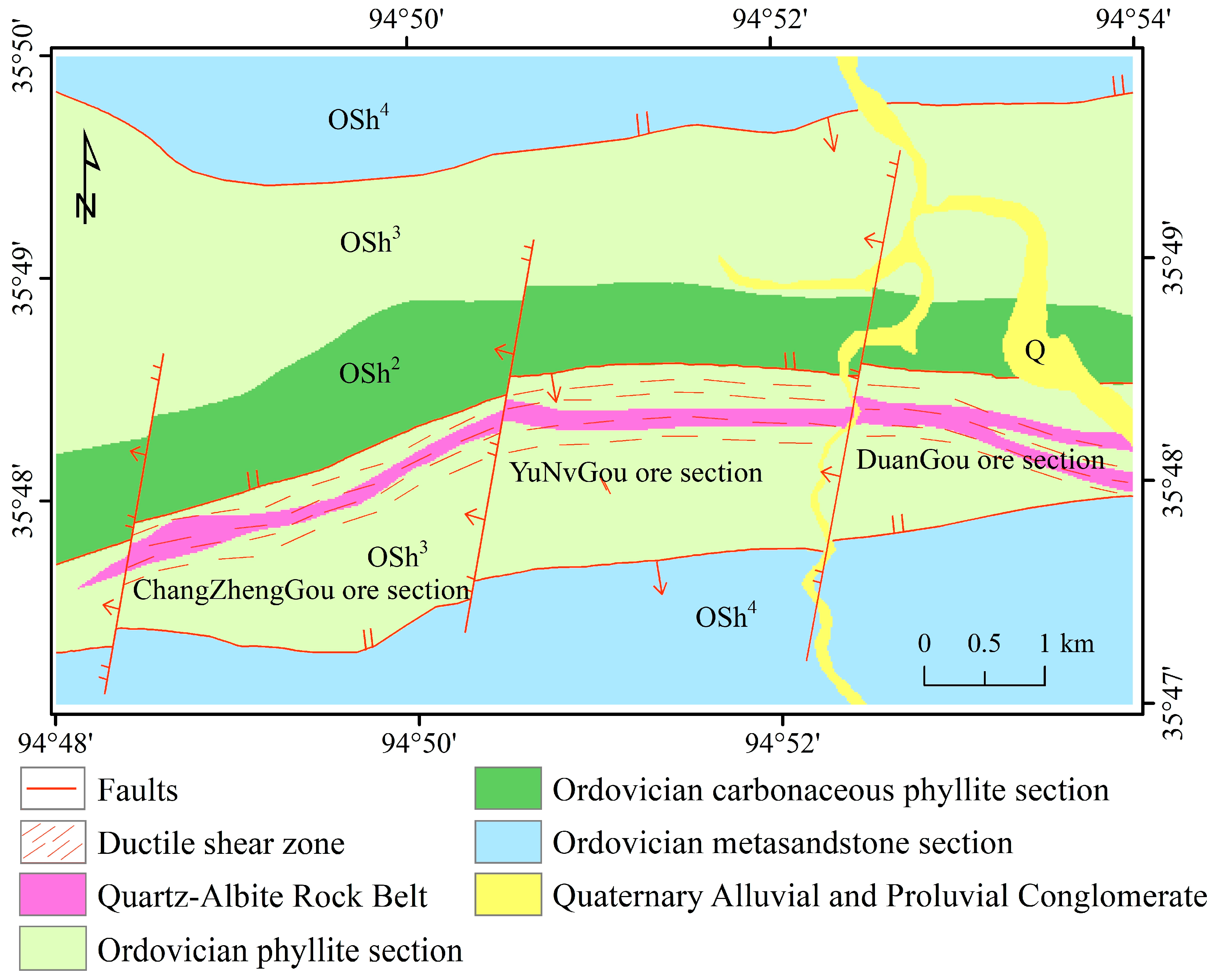
2. Geological Background

The Tuolugou mining area is located within the East Kunlun orogenic belt, specifically in the active zone of the southern Kunlun continental margin. As shown in Figure 1, the exposed strata in the area primarily consist of three lithological sections from the Ordovician Nachitai Group: the carbonaceous phyllite (OSh2), the phyllite (OSh3), and the metasandstone (OSh4). OSh2 is mainly composed of carbonaceous phyllite, carbonaceous slate interbedded with siltstone, and thin-layered limestone. OSh3 is chiefly composed of chlorite–sericite–quartz schist, quartz–albite rock, and sericite-quartz schist. OSh4 mainly consists of metasandstone, metaconglomerate, quartz–albite rock, chlorite–sericite–quartz schist, and siliceous rock [27]. In addition to these three lithological sections, a Co (Au)-bearing quartz–albite belt and Quaternary sediments have developed in the Tuolugou area.
The Tuolugou mining area is situated between the Kunzhong and Kunnan Faults. Influenced by Indosinian–Yanshanian N–S compression, the regional strata strike, structural trends, and dike orientations are predominantly E–W. The area is characterized by folds and fault zones, with faults mainly divided into two groups: those near E–W-trending structures and those near N–S-trending structures. The faults near E-W-trending structures consist of thrust faults subparallel to the strata strike or fold axes. These faults exhibit stable along-strike extension, steep dips, and northward orientation. In contrast, the faults near N–S trending structures are post-mineralization structures. Based on the displacement of E–W trending strata and the geometry of the faults, three major faults near N–S-trending structures in the mining area have been identified as steeply west-dipping normal faults. Additionally, the mining area exhibits intense plastic deformation, manifested as an E–W-trending ductile–brittle shear zone. The ductile deformation is large-scale, forming foliation zones and mylonite belts. Rocks within these zones display dense foliation, cleavage, and pronounced recrystallization, with newly formed metamorphic minerals such as sericite and chlorite. Brittle fractures, serving as subsidiary structures controlled by the ductile shear zones, are marked by cataclastic rocks and fault gouges. These structures provided pathways and space for later ore-bearing hydrothermal fluids, directly controlling orebody emplacement.

3. Data and Methodology

3.1. Remote Sensing Data

Hyperspectral imaging (HSI), a typical form of Earth-observation data, consists of hundreds of contiguous spectral bands, providing abundant spectral information for each pixel of the ground targets [30]. The GF5B satellite is equipped with seven payloads, and the Advanced Hyperspectral Imager (AHSI) consists of 330 spectral channels covering a spectral range of 387–2515 nm [31]. Compared with other hyperspectral data, the GF5B satellite data have the characteristics of a higher signal-to-noise ratio, enhanced spectral curve details, and less fringe noise [32,33] (Table 1). The numerous spectral channels of the hyperspectral observation satellite facilitate the expansion from analyzing geometric shapes and color perception to extracting detailed spectral information, thereby opening a new chapter in the field of geological prospecting [34]. This study utilized the hyperspectral data obtained from the Advanced Hyperspectral Imager (AHSI) aboard the GF5B satellite, as well as the multispectral data from the multitemporal Landsat-8. Landsat remote sensing data was selected for lithological mapping mainly due to the advantages of multi-temporal data and easy access. It has been shown that external environmental factors, such as temperature and humidity, have a significant impact on lithology identification, and it is difficult for single-time-phase data to fully reflect these changes. Multi-temporal remote sensing data can reduce classification noise in the time dimension, thus providing image information that is more stable. Although the spectral resolution of AHSI hyperspectral data from GF5B is high, it is expensive, while Landsat-8 remote sensing data are freely available. Therefore, in this study, we chose multi-temporal Landsat-8 images from 2013 to 2021 with the aim of extracting features such as temperature, wetness, greenness, and brightness to improve the accuracy of remote sensing-based lithology identification.
Remote sensing technology can enable extensive surface observations over large areas in a short time, which facilitates the classification of different rock types by the capture of various spectral and textural details from the rock surfaces [35]. The influence of external factors may be beneficial for lithology identification in remote sensing imagery. For example, in the southern part of the Tuolugou mining area, the quartz albite has a lower heat capacity, which may lead to higher temperatures in thermal imaging. The dense structure of carbonaceous phyllite and carbonaceous slate hinders the infiltration and retention of water, which makes them unfavorable for vegetation growth and likely results in lower wetness and greenness. When single-temporal remote sensing data are used for rock classification, determining the influence of external changes on rock image features (such as wetness and temperature) is difficult. In contrast, multitemporal remote sensing data can balance the influence of external environmental and climatic factors, reducing classification noise from a temporal perspective, and thereby providing image information which is more stable [36]. In this study, Landsat-8 imagery from 2013 to 2021 was acquired to extract four features of the remote sensing images, namely, temperature, wetness, greenness, and brightness. These features, which show significant temporal changes and continuous spatial distributions, were used for lithology identification using remote sensing. In order to minimize the influence of clouds and snow, the images selected ranged from mid-May to early October, a period in which the overall cloud cover of each image was less than 10%, and there was no cloud cover over the study area.

3.2. Preprocessing of the Remote Sensing Data

Preprocessing of remote sensing data involves correcting various distortions and deformations in the images to obtain a more informative and realistic representation. The preprocessing steps typically include radiometric correction, geometric correction, and image cropping.

3.2.1. GF5B Hyperspectral Data

The GF5B satellite carries seven payloads, including the visible shortwave infrared hyperspectral camera (AHSI), which has a total of 330 spectral channels within a spectrum range of 387–2515 nm and a spectral resolution of up to 5 nm (Table 2).
However, due to water vapor absorption effects, bands 193–200 and 246–262 were invalid, and thus were removed [37]. Additionally, spectral overlap was observed between the visible/near-infrared (VNIR) bands (145–150) and the shortwave infrared (SWIR) bands (151–153). Given the higher signal-to-noise ratio (SNR) of the VNIR bands compared to the SWIR bands, the latter (151–153) were discarded to retain superior data quality [38]. Furthermore, the last five SWIR bands (326–330) exhibited significant noise and were consequently excluded to avert their adverse impacts on data integrity.
A thorough band-by-band inspection revealed that certain bands contained defective line stripes. For isolated bad lines, pixel values were corrected using the average of adjacent columns/rows [39], while stripe noise was addressed via a global describing algorithm [40]. Although some bands showed marked improvement after restoration, others retained persistent artifacts and were deemed unusable. In total, 37 bands were eliminated, resulting in 293 retained bands (Table 3).
Radiometric correction consists of two key steps: radiometric calibration and atmospheric correction. Radiometric calibration serves as the prerequisite for atmospheric correction, converting the raw digital numbers (DN) recorded by the sensor into physically meaningful units such as radiance, reflectance, or temperature [24]. This process mitigates distortions introduced by sensor-specific characteristics. Atmospheric correction, on the other hand, aims to minimize the interference caused by atmospheric effects (e.g., scattering and absorption) in the electromagnetic radiation reflected or emitted by surface features, thereby recovering the true spectral properties of targets [41]. For this study, radiometric calibration and atmospheric correction were performed using ENVI software (version 5.3), specifically, its radiometric calibration tool and the FLAASH module. To optimize computational efficiency, the GF-5B image was subset to focus on the study area, avoiding unnecessary processing of the entire scene.
While GF-5B offers exceptional spectral resolution (up to 5 nm), its spatial resolution is limited to 30 m. In contrast, multispectral and panchromatic (PAN) imagery typically provides coarser spectral but finer spatial resolution, capturing richer geometric details. Leveraging auxiliary data from PAN or multispectral sources can thus enhance the spatial resolution of hyperspectral imagery through fusion techniques. This study adopted hyperspectral–panchromatic fusion (pansharpening), which integrates low-resolution hyperspectral data with high-resolution PAN imagery (15 m from Landsat-8) to generate high-resolution hyperspectral output. From among prevalent fusion methods (e.g., Color Normalization, PCA, and Gram–Schmidt (GS)), the GS transform was selected for its ability to preserve spectral fidelity while improving spatial detail. The method circumvents band limitations and effectively retains spatial textures, ensuring minimal distortion of the original GF-5B spectral features. As a result, a high-resolution hyperspectral image with 293 bands and a spatial resolution of 15 m was obtained in the Tuolugou mining area.

3.2.2. Landsat-8 Multispectral Data Preprocessing

The temperature, wetness, greenness, brightness, and texture features were extracted from the multitemporal Landsat-8 images after radiometric correction, geometric correction, and image cropping. The temperature data were obtained from band 10 of the Landsat-8 images using the single-channel algorithm [42], whereas three typical surface features, wetness (TCTW), greenness (TCTG), and brightness (TCTB), were extracted by the tasseled cap transformation (TCT) method [43]. The TCT component is calculated by weighted summation of different bands, and can show the surface properties from different aspects. Under certain circumstances, TCT components can reflect 95% of the changes in the original image [44]. Another advantage of TCT transform is that its coefficient does not change with the images, so researchers can directly compare the results of TCT transforms within a multi-temporal image [45]. Landsat-8 multispectral imagery from 2013 to 2021 was separately fused with the corresponding panchromatic images, while ensuring that the images had the same spatial resolution as the GF5B hyperspectral imagery. The average of the four features was then calculated to obtain the yearly feature image averages across the duration (Figure 2).
As a primary visual attribute of rock units, the texture reveals differences in physical weathering and drainage, providing auxiliary information useful in distinguishing rock types [8]. Owing to the stability of the texture features [36], the Landsat-8 images from 2021 were used to extract eight texture features with the grey level co-occurrence matrix (GLCM) method [46], as shown in Figure 3.

3.3. Principles of Convolutional Neural Networks

3.3.1. Convolutional Neural Network

Convolutional neural networks (CNNs) have garnered particular attention because of their unique advantages [47]. The architecture of a CNN usually consists of input layers, convolutional layers, pooling layers, fully connected layers, and activation functions, which together automatically extract the high-level features, layer-by-layer [48]. The convolutional layer is the core component of the CNN, typically consisting of one or multiple convolutional kernels, while the primary purpose of the convolutional layer is to extract features from the input at different levels [49]. The main function of the pooling layer is to downsample feature maps. The pooling layers commonly used in image classification problems include max pooling and average pooling [50]. Fully connected layers are typically located at the end of a CNN. Their main function is to transform the features extracted by the previous convolutional and pooling layers into a one-dimensional vector, enabling a nonlinear combination of features.

3.3.2. The Dual-Channel Convolutional Neural Network

CNNs are neural networks specifically designed to process data with a grid-like structure, such as one-dimensional time series data or two-dimensional and three-dimensional image data [51]. Particularly with remote sensing imagery, CNNs are capable of extracting both the spectral and spatial features during image processing, thereby enabling a more comprehensive understanding of the data’s intrinsic properties [52]. However, traditional CNNs typically have a single-branch structure that can extract only one kind of spectral feature or spatial feature first, before extracting the other kinds. The limited interaction between these two processes may result in an inadequate extraction of data with both spectral and spatial information. Therefore, this study proposes a dual-channel convolutional neural network model (DC-CNN) which simultaneously extracts the spectral and spatial features from remote sensing images. While analyzing the spectral information of each pixel, the model also considers its spatial context. The DC-CNN comprises two channels: the first channel uses a 1D-CNN to learn the spectral features of the hyperspectral images, whereas the second channel uses a 2D-CNN to learn the spatial features of the multitemporal multispectral images.
In this model, the spectral feature channel uses a one-dimensional convolutional neural network (1D-CNN) in which the input and output data are two-dimensional, and the kernel slides along one direction. In hyperspectral image classification, since the spectral information is one-dimensional, a 1D-CNN is commonly used for extracting spectral information [53]. The spatial feature channel uses a two-dimensional convolutional neural network (2D-CNN). The 2D-CNN captures spatial information through two-dimensional convolutions, and has been widely used for hyperspectral image classification, achieving good classification accuracy [54,55]. The features output from the two channels are subsequently concatenated into a combined feature vector that contains spectral and spatial information, thus implementing lithology identification through feature fusion. The detailed structure of the model is introduced in Section 4.2.

3.4. Random Forest

Random Forest is an ensemble learning method based on decision trees. It constructs multiple decision trees and aggregates their predictions through voting mechanisms. By introducing randomness, Random Forest effectively reduces the variance of individual decision trees, demonstrates strong noise tolerance, and significantly enhances model robustness. The core principles of Random Forest involve two key randomization processes:
(1)
Bootstrap aggregation (bagging): Random sampling with replacement from the original training data to create K subsets.
(2)
Feature subspace selection: For each subset, randomly choosing N features for model construction.
This dual randomization approach generates K distinct decision trees, whose classification results are subsequently combined through majority voting. The ensemble framework capitalizes on the strengths of multiple decision trees, substantially improving classification accuracy. The algorithmic workflow proceeds as follows:
(1)
Randomly select a portion of features for decision tree construction to ensure the diversity of the evaluation model.
(2)
For each subset of features, apply the recursive partitioning method to construct the corresponding decision tree to eliminate the uncertainty of the samples in each leaf node. Repeat the above steps to form a random forest.
(3)
In classification problems, the majority voting method is used to derive the final prediction results, while in regression problems, the average value method is utilized to obtain the final prediction results.
(4)
Evaluate the model using relevant evaluation metrics and adjust the parameters to optimize the performance of the model.

3.5. Evaluation Metrics

To quantitatively assess the effectiveness of the model in lithology identification, this study uses a confusion matrix to evaluate the accuracy of the classification results. The confusion matrix method has been widely used for accuracy assessments in supervised classification of remote sensing images across different regions, scales, and thematic studies [56,57]. By tallying the number of correct and misclassified pixels for each lithology category in the study area, the confusion matrix allows for the calculation of various accuracy metrics, such as overall accuracy (OA), average accuracy (AA), and the kappa coefficient [58].
(1)
Overall Accuracy (OA)
Overall accuracy is defined as the ratio of the number of correctly categorized pixels to the total number of pixels.
O A = n = 1 N T P i M
(2)
Average Accuracy (AA)
For each class, the classification accuracy is defined as the ratio of the number of correctly classified pixels for that class in the test set to the total number of pixels belonging to that class. The average accuracy (AA) is calculated as the mean classification accuracy across all the classes in the image.
A A = 1 N n = 1 N T P i T P i + F N i
(3)
Kappa coefficient
The kappa coefficient is an indicator used to measure the agreement between model predictions and actual classification results. It is commonly used to assess the quality of the overall classification performance. In general, the kappa coefficient lies between 0 and 1, with larger kappa values indicating higher classification accuracies.
K appa = N 2 O A n = 1 N T P i + F N i T P i + F P i N 2 n = 1 N T P i + F N i T P i + F P i
In Equations (1)–(3), N represents the number of categories, M is the total number of samples, TPi is the number of true positive samples for the ith category, FNi is the number of false negative samples for the ith category, FPi is the number of false positive samples for the ith category, TPi + FNi represents the total number of actual samples for the ith category of the confusion matrix, and TPi + FPi represents the total number of predicted samples for the ith category of the confusion matrix.

3.6. Shapley Additive Explanation

Deep learning models are capable of achieving powerful performance because of their complex architectures. However, owing to the complexity of these models, gaining a comprehensive understanding of the relationship between the input features and output results is challenging; this leads to a lack of interpretability in the predictions. These models are often termed “black box” models [59,60]. To enhance the interpretability of deep learning models, various explainability methods have been proposed. For example, model transparency can be solved through visualization techniques [28,61,62], and neural networks can be explained at the feature level [63,64].
SHAP (Shapley additive explanations), initially proposed by Lundberg (2017), is a post hoc interpretation method [65]. On the basis of cooperative game theory, SHAP provide model explanations by treating input features as “contributors” to the prediction outcome. By calculating the SHAP value for each feature, this method quantifies the magnitude and direction of each feature’s impact on the prediction outcome, thereby assessing feature importance and enhancing the interpretability of the deep learning models. The calculation formula for the SHAP value φi of feature Xi is as follows:
φ = S N \ i S ! N S 1 ! N ! f S i f S
where N represents the set of all features, denoted as (X1, X2, …, XM); S is a subset of N that does not contain feature Xi; |S| represents the size of the subset S; and f(S) denotes the predicted output of the model when only the features in subset S are included. Similarly, f(S∪{i}) represents the model’s output when both S and feature Xi are included. First, for each feature Xi, we iterate through all feature subsets S that do not contain Xi. Then, we separately calculate the predicted output when using only the feature subset S (without Xi) and the predicted output f(S∪{i}) when including Xi in subset S, thereby obtaining the difference in the predicted output f(S∪{i}) − f(S); this represents the difference between the model outputs in the cases of including and not including feature Xi, thus quantifying the marginal contribution of feature Xi. Finally, to ensure the fair evaluation of each feature’s marginal contribution, the marginal contributions of all possible subsets S are weighted and summed to obtain the SHAP value φi of feature Xi, which represents the contribution of feature Xi to the model’s output.

4. Model Construction Based on Remote Sensing Data

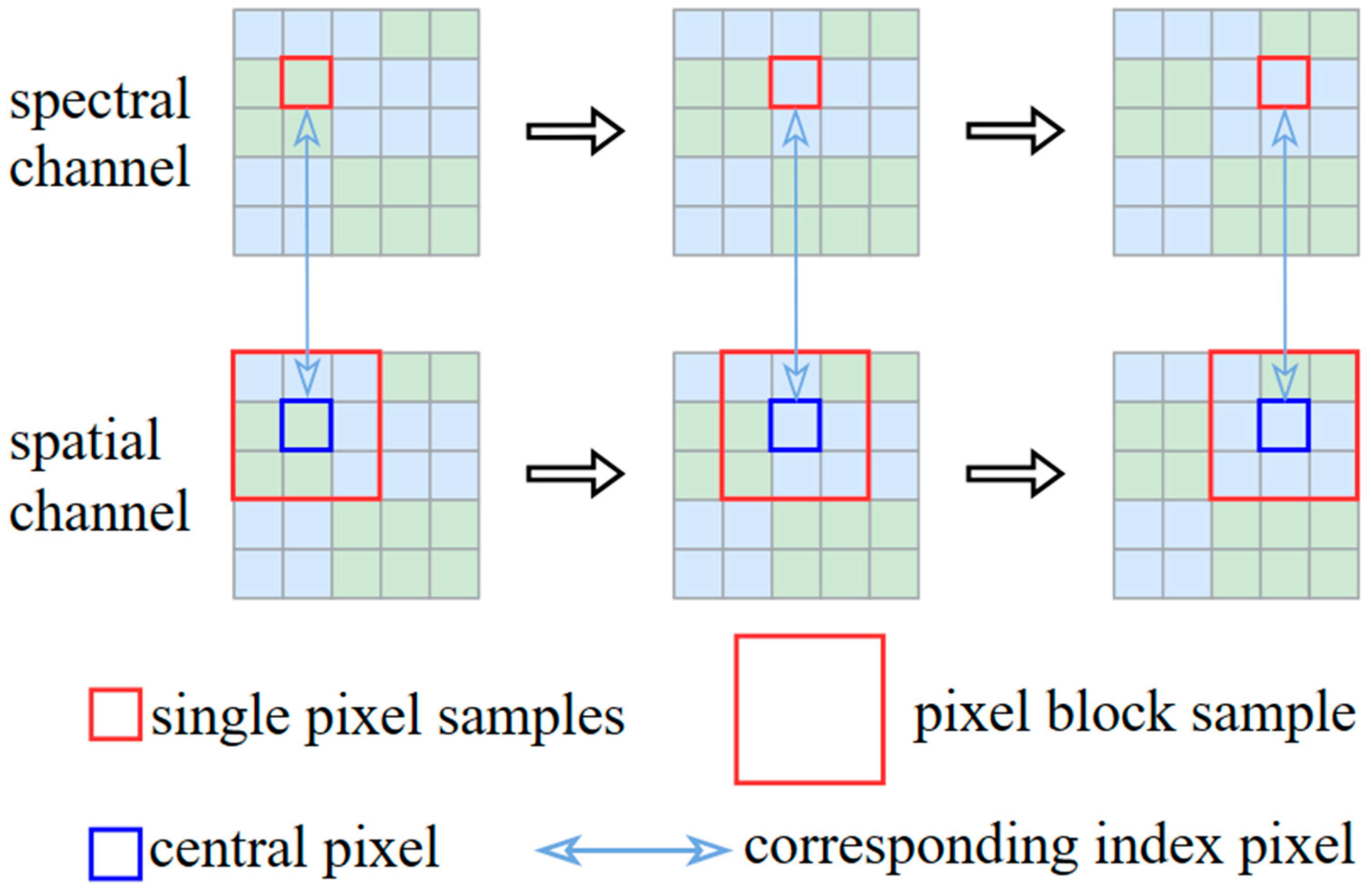
4.1. Sample Production

After data preprocessing, the GF5B hyperspectral image and multitemporal Landsat-8 images were both adjusted to a size of 595 × 359 pixels, with a spatial resolution unified to 15 m, covering an area of approximately 48 km2. The GF5B hyperspectral image comprises 293 bands, constituting the spectral features, whereas the spatial feature extracted from the multitemporal Landsat-8 image contains 12 bands. A schematic illustrating the sample generation process is presented in Figure 4.
The goal of remote sensing image classification is to assign a label to each pixel in the image [66]. Thus, it is necessary to ensure that the pixels in both the GF5B hyperspectral image and the Landsat-8 image are geographically aligned. For the GF5B hyperspectral image, each pixel was processed individually to construct pixel-based samples, with each sample comprising 293 spectral bands. Simultaneously, for the spatial feature images, each pixel is traversed, and pixel blocks centered on the current pixel are constructed as samples. Each pixel block contains 12 types of spatial features, and the label of the center pixel is used as the reference. Subsequently, based on the distribution of the lithology units, one-third of the pixels and corresponding pixel blocks are selected as the samples of the two channels. In total, approximately 78,000 sets of single-pixel samples and pixel block samples were selected, and these were then divided into training and validation subsets at a ratio of 8:2.

4.2. Construction of the Dual-Channel CNN Model

The dual-channel convolutional neural network model (DC-CNN) developed in this study consists of two primary channels. The first channel uses one-dimensional convolution (1D-CNN) to extract the spectral features of the GF5B hyperspectral image. The second channel uses two-dimensional convolution (2D-CNN) to extract the spatial features from the multitemporal Landsat-8 images. The features extracted from the two channels are concatenated into a joint feature vector, thus enabling lithology identification through remote sensing.

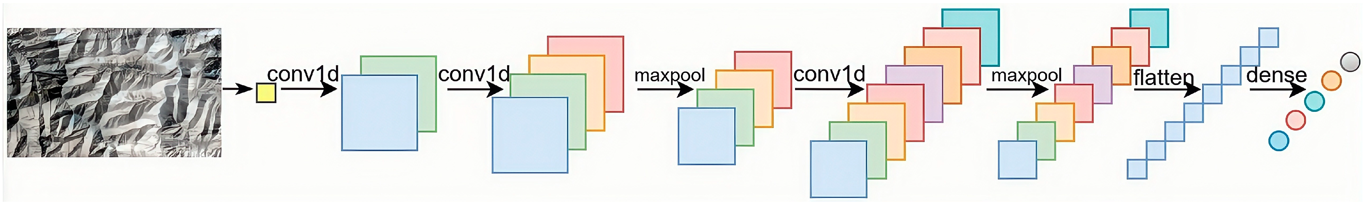
4.2.1. The Spectral Feature Channel

By extracting one-dimensional spectral information, the 1D-CNN can utilize interband differences to classify the targets in the image. The structural parameters of the spectral feature channel are listed in Table 4, with a schematic diagram shown in Figure 5. The spectral feature channel consists of three one-dimensional convolutional layers, two max pooling layers, a flatten layer, and a fully connected layer. First, the channel receives the spectral profile of a single pixel from the hyperspectral image, and the original spectral features consisting of 293 bands are extracted by two convolutional layers. Second, a max pooling layer is employed to reduce the dimensionality of the output features, which helps to mitigate the risk of overfitting and decreases the computational complexity. Third, another convolutional layer is used to learn the downsampled spectral features; this is followed by another max pooling layer for additional downsizing. Finally, the flatten layer converts the output features into a one-dimensional vector, which is fed into a fully connected layer for learning deeper spectral features. The result of this fully connected layer represents the final output of the spectral feature channel.

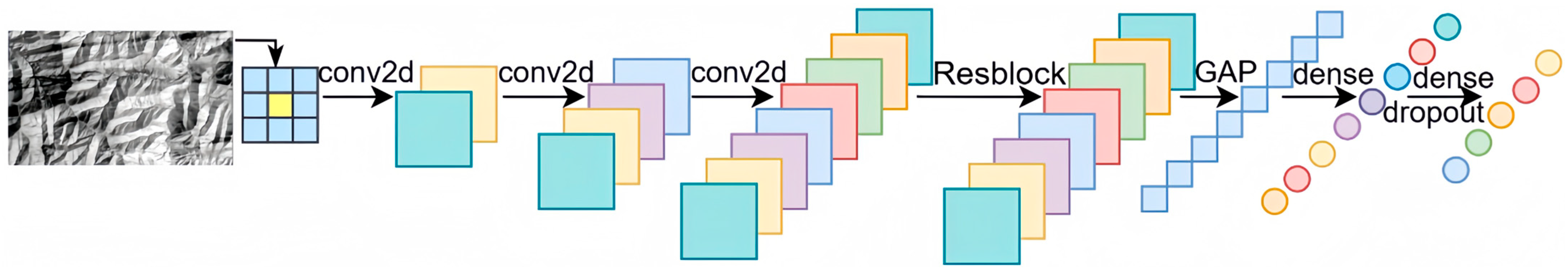
4.2.2. The Spatial Feature Channel

The 2D-CNN can analyze the neighboring features of the pixel blocks, thereby extracting spatial information from the image. The structural parameters of the spatial feature channel are listed in Table 5, with a schematic diagram shown in Figure 6. The spatial feature channel consists of three two-dimensional convolutional layers, a residual block, a global average pooling layer, and two fully connected layers. The channel receives a 5 × 5 pixel block constructed around a single pixel at the center. First, two-dimensional convolutional layers are used to extract 12 spatial features from each pixel block; these are followed by an additional convolutional layer to capture the more complex features. Generally, the deeper the network is, the stronger its ability to extract feature information. However, simply increasing the network’s depth may lead to issues such as gradient vanishing and network degradation [67]. Therefore, a residual block is added after the three convolutional layers. The residual network (ResNet) uses skip connections to map shallow features. Without any additional parameters or increased computational complexity, this architecture addresses the issues of gradient vanishing and network degradation caused by deeper networks [68]. Second, the output features of the residual block are reduced to a one-dimensional vector through a global average pooling layer. Third, the dimension-reduced features are fed into two fully connected layers in which the dropout technique is applied to reduce overfitting and enhance model generalization. Finally, a fully connected layer containing 128 neurons is used to compress and integrate the feature information, and the resulting output serves as the final representation of the spatial feature channel.

4.2.3. Feature Integration

A single-branch network structure may lead to the spectral and spatial features of the remote sensing data existing in different domains, which could disrupt the extracted features [69]. Therefore, the model adopts a parallel dual-channel structure to extract the spectral and spatial features simultaneously. The structural parameters of the spectral feature channel are listed in Table 6, and its schematic diagram is shown in Figure 7. First, the spectral and spatial feature vectors output by the two channels are concatenated along their feature dimensions. Second, the concatenated joint feature vector is passed to a fully connected layer, in which the features are combined by linear transformation and nonlinear activation. Finally, the combined features are fed into another fully connected layer, in which the final lithology prediction labels are generated using the softmax activation function.

5. Results

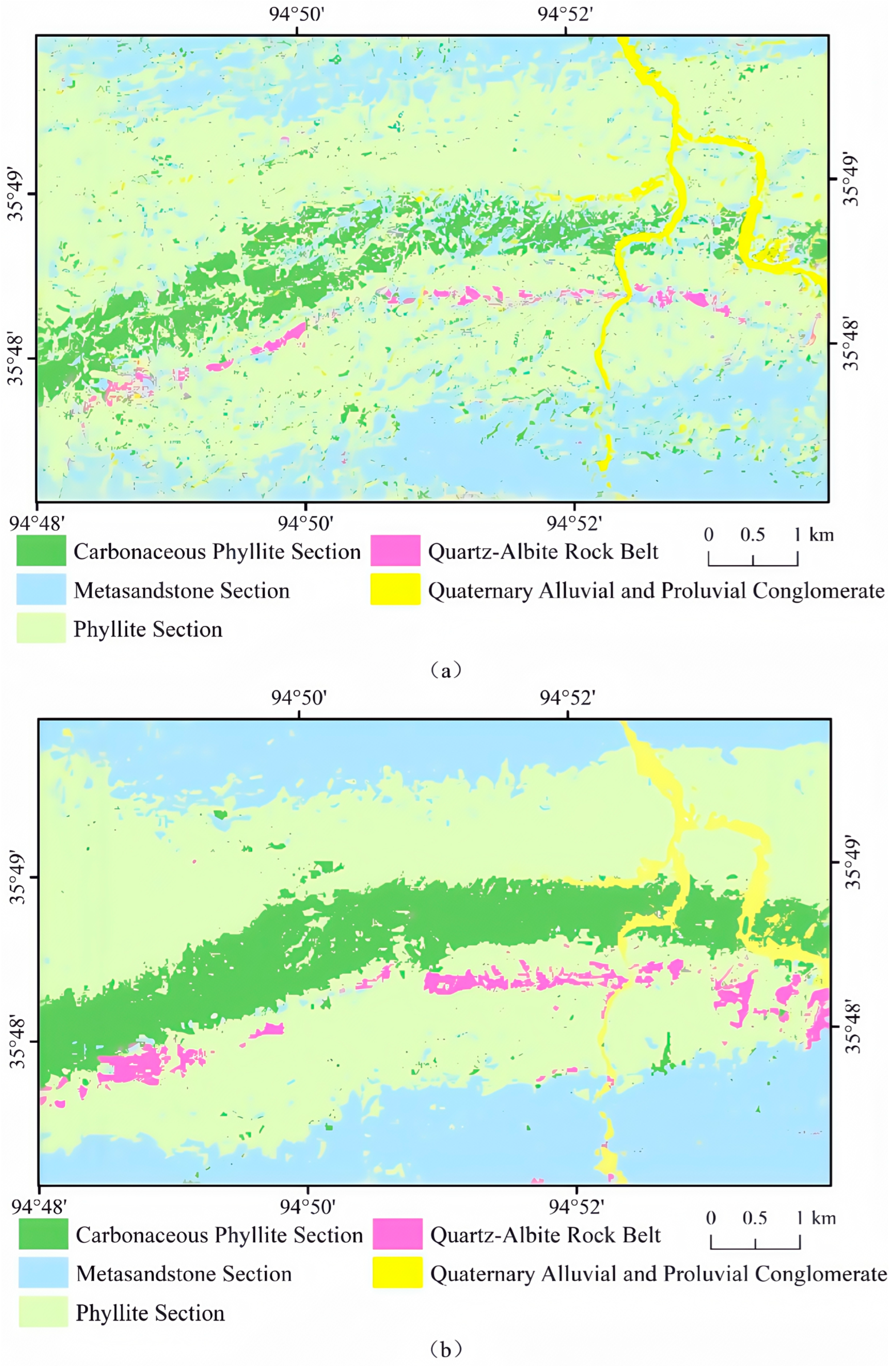
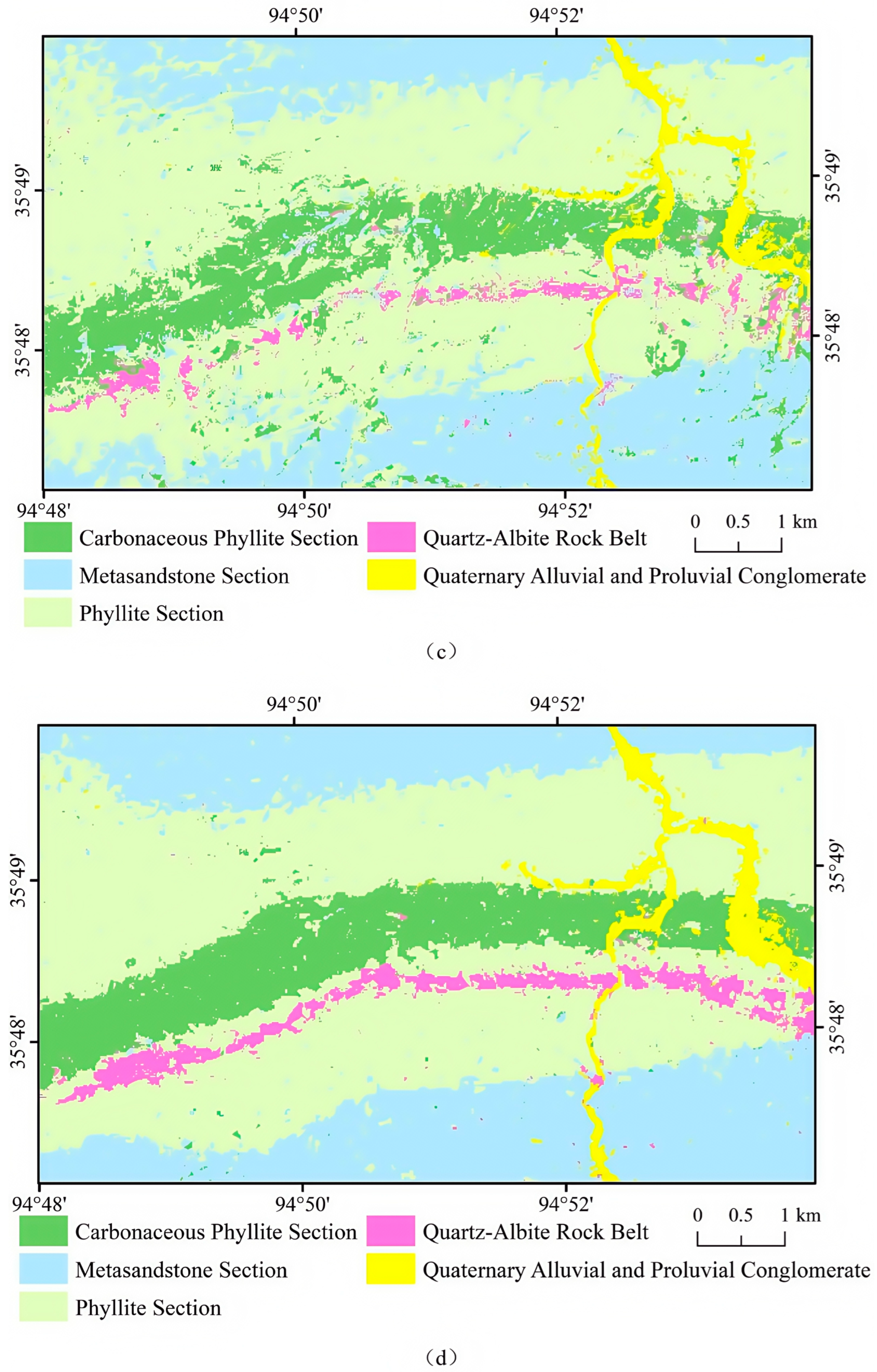
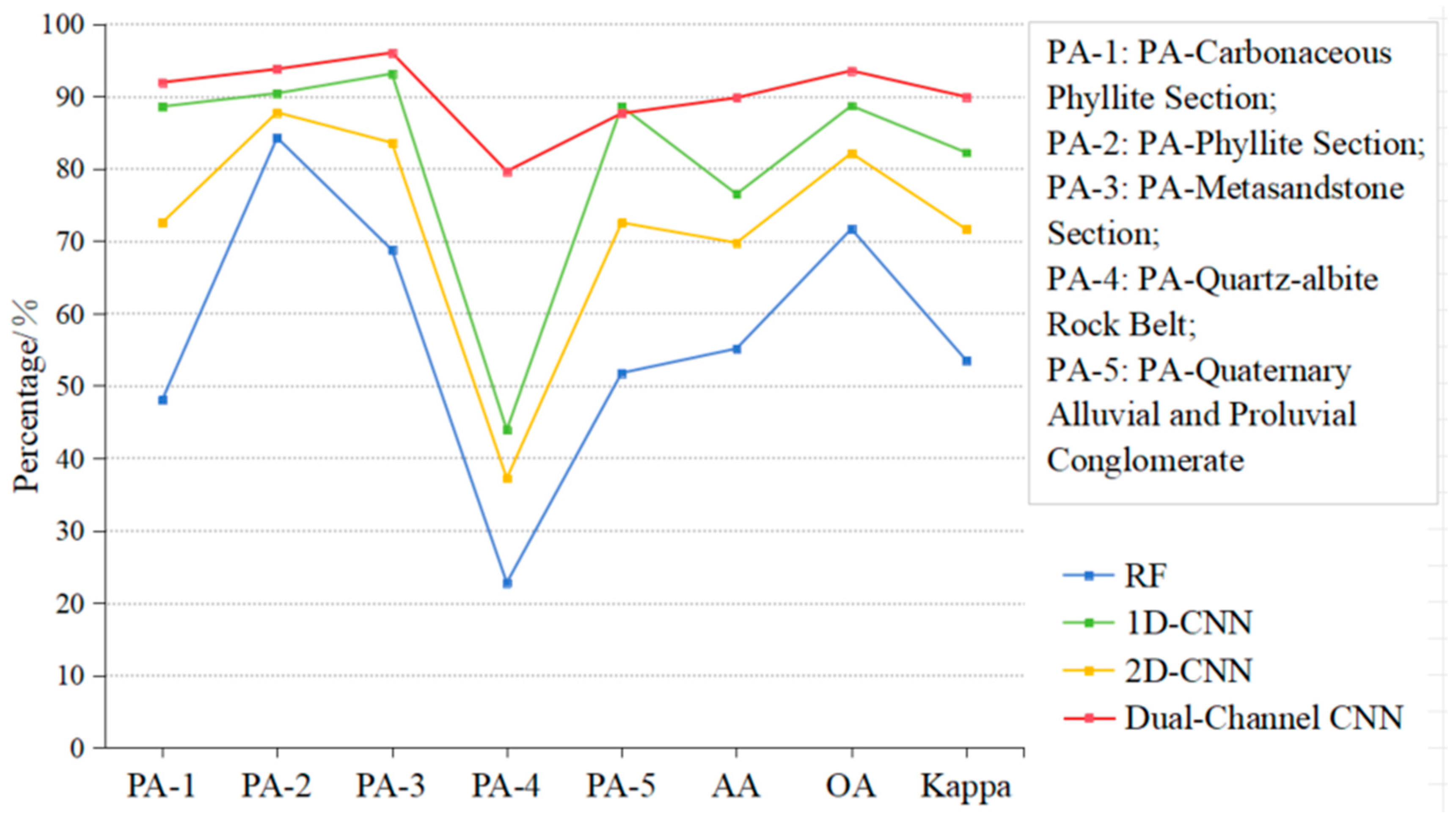
5.1. CNN-Based Lithology Identification and a Comparative Analysis

Five lithology units were identified by the DC-CNN model in the Tuolugou mining area. To validate the lithology identification accuracy of the DC-CNN model, it was compared with other algorithms: the 1D-CNN, 2D-CNN, and RF algorithms. To assess the classification performance and minimize the impact of experimental randomness, all the models were trained for 10 epochs, and the best-performing results were selected for a comparative analysis. The experiments of the four models were conducted under the same computer environment, and the sample set was divided into equal proportions to enhance the comparability of the results.
Figure 8 shows the lithology identification results generated by the four models. The RF model exhibits the poorest performance, particularly in the identification of the carbonaceous phyllite section and quartz–albite, leading to significant misclassification issues. It identifies only a small portion of the pixels correctly, resulting in an overall accuracy that is significantly lower than those of the other models (Figure 8a). The 1D-CNN model can effectively distinguish different lithologies overall, however, its accuracy is relatively low in local areas, resulting in confusion between the carbonaceous phyllite section and the phyllite section (Figure 8b). In the prediction results of the 2D-CNN model, the misclassification of pixels among the carbonaceous phyllite section, phyllite section, and metasandstone section becomes more pronounced, and the 2D-CNN struggles to distinguish the boundary between the phyllite section and metasandstone section (Figure 8c). The DC-CNN model accurately identifies five lithological units, with clear lithological boundaries in the predicted results and relatively few misclassified pixels within each unit (Figure 8d). Additionally, both the 1D-CNN and 2D-CNN models have difficulty accurately identifying quartz–albite, whereas the DC-CNN model effectively recognizes most of the quartz–albite. This further demonstrates that the dual-channel network structure, which can extract the spectral and spatial features separately, has significant advantages over single-channel networks. Compared with those of the other three models, the classification results of the DC-CNN model are very close to the actual geological map, especially in classifying the quartz–albite rock belt. Thus, the DC-CNN model has the best performance in lithology identification for the Tuolugou mining area.
This study then evaluated these models. The classification accuracies calculated from the confusion matrices show that the accuracy of the Random Forest model is the lowest; in particular, the identification accuracy for the quartz–albite belt is only 22.79%, with only a small portion of the pixels correctly identified (Table 7). On the other hand, the three CNNs achieve significant improvements in accuracy over the RF model, suggesting that the traditional machine learning models, such as the RF model, can extract only shallow features. Spatial structures, local textures, and other information in the images may be overlooked or inadequately identified by the RF model. In contrast, with their unique structure and feature-extraction mechanisms, CNNs can better capture complex patterns in images and learn deep spectral and spatial features. Among the three CNN models, the accuracy of the DC-CNN model is the highest, and the overall accuracy (OA) of the DC-CNN model is 93.51%, with an average accuracy (AA) of 89.77% and a kappa coefficient of 0.8988. Among the five lithological units, the DC-CNN model achieves classification accuracies above 85% for all units except for the quartz–albite unit, and the lithological boundaries are relatively clear, with fewer misclassified pixels. The relatively lower classification accuracy (79.62%) for quartz–albite may be attributed to both the metasandstone and phyllite sections containing some quartz–albite, as well as the limited distribution area of quartz–albite. Even so, as shown in Table 6, the DC-CNN model significantly improves the identification accuracy for quartz–albite compared with the other models. Figure 9 shows that the DC-CNN model consistently outperforms the other three models, except in the classification of Quaternary alluvial and proluvial conglomerate. The results indicated that the identification ability of the DC-CNN model can be improved markedly by combining the spectral features and spatial features.
Previous studies have suggested that the Tuolugou mining area is promising for cobalt exploration, and several hydrothermal ore-bearing cobalt deposits have been discovered [70]. The ore bodies are primarily hosted in phyllite and metasandstone formations, with quartz–albite rocks serving as the main ore-hosting lithology in the Tuolugou mining area. Therefore, accurately identifying ore-hosting quartz–albite rocks not only increases the understanding of the mineralization mechanism of this deposit but also provides a model application example and essential technical support for cobalt exploration in similar regions. However, Table 5 shows that the classification accuracies of the RF, 1D-CNN, and 2D-CNN models for quartz–albite are 22.79%, 43.90%, and 37.20%, respectively. These models can barely recognize half of the quartz–albite, with a large portion of the pixels misclassified as phyllite. In contrast, the DC-CNN model improves the accuracy to 79.62%, and accurately identifies the overall orientation of the quartz albite. The comparison results further imply that comprehensive lithology identification achieved by combining the spectral features and spatial features of the remote sensing images is more efficient than the traditional remote sensing lithology mapping methods that consider only the spectral or spatial features.

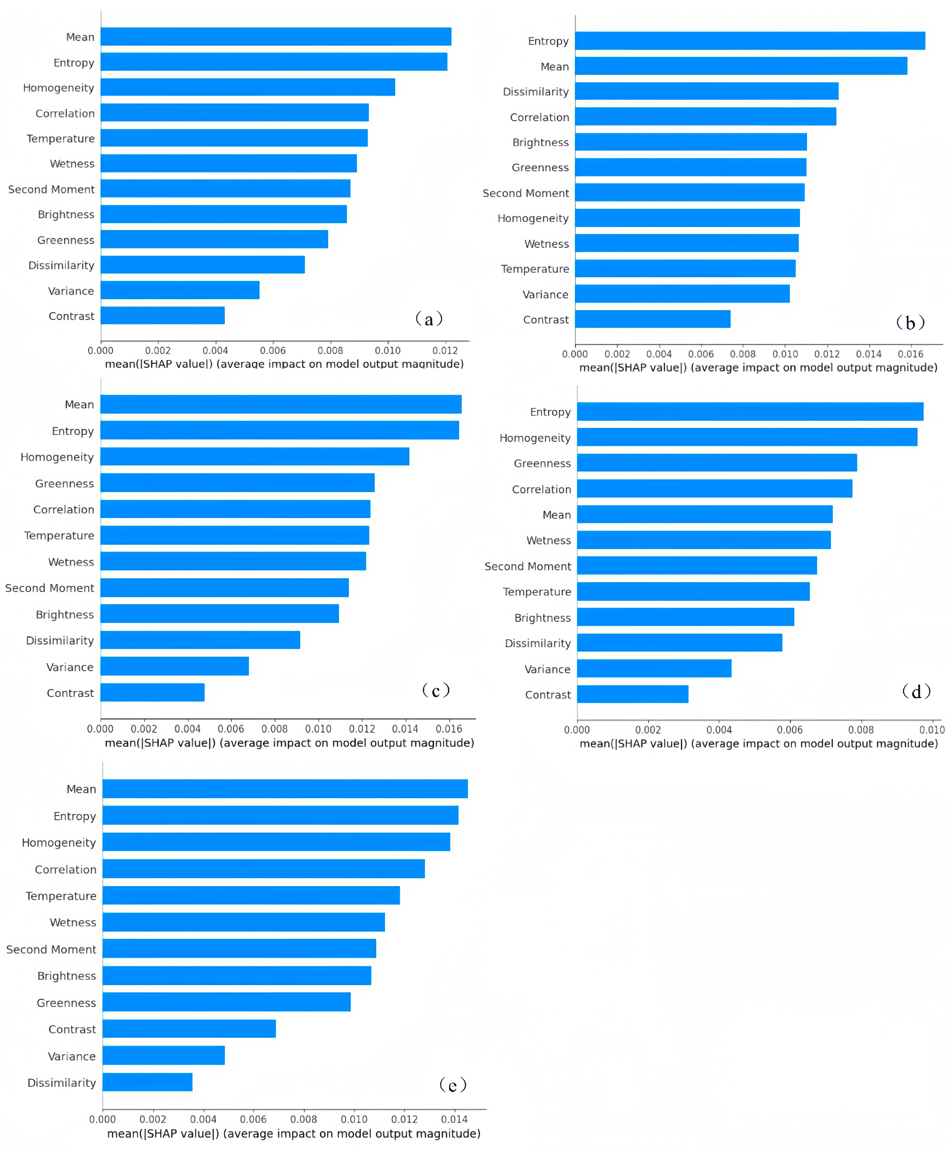
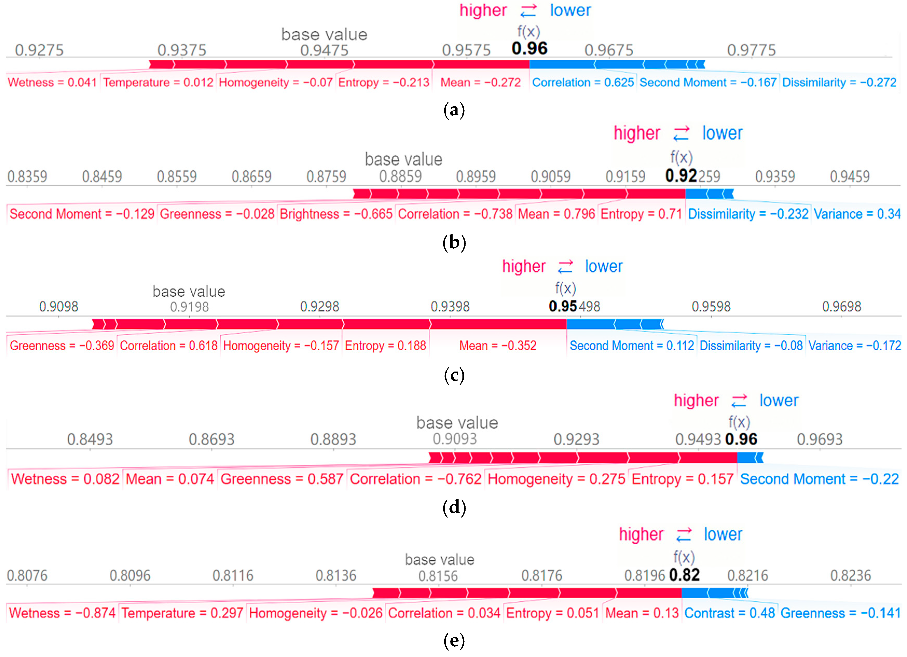
5.2. SHAP Method for Lithology Interpretation

The SHAP method provides global explanations for all the samples, and local explanations for the individual samples. SHAP feature-importance charts are used to interpret the five lithological units globally, thus obtaining the contribution magnitudes of the individual features. Moreover, the average SHAP force plots are utilized to investigate the direction of the contributions of these features to the correct identification by the DC-CNN model. This approach was employed to elucidate, from the perspective of the magnitude and direction of feature contributions, whether the four external environmental features introduced in this study contribute to the improvement of remote sensing lithological identification accuracy. The SHAP feature-importance chart is created by taking the mean absolute value of the SHAP values for each feature, producing a standard bar chart that explains the predictions for all the samples. This chart displays the absolute contribution of each feature to the model without indicating the direction of the feature contributions. This chapter focuses on explaining the 12 spatial features used in the spatial feature channel of the models, visualizing the magnitudes and directions of the contributions of these features. Moreover, this chapter aims to demonstrate the introduction of temperature, brightness, wetness, and greenness, which have rarely been considered in the past but are helpful for the prediction of lithology identification in the remote sensing images, thereby highlighting the model interpretability.
The DC-CNN model constructed in this study utilizes 12 spatial features in the spatial feature channel, which can be classified into eight texture features (i.e., mean, variance, homogeneity, contrast, dissimilarity, entropy, second moment, and correlation) and four multitemporal features (i.e., temperature, wetness, greenness, and brightness). As shown in Figure 10, the SHAP feature-importance charts for the 12 spatial features were generated from the samples of the five rock type units in the test set. The features such as mean, entropy, and homogeneity are usually in the top three in the identification among the five lithology categories, indicating that these texture-based features can better capture the surface structural features of the lithology samples, and they play a major role in the lithology identification using the remotely sensed imagery. In addition, temperature, wetness, greenness, and brightness also make a certain contribution to the identification processes of the different lithology units, respectively. These results show that the four features of temperature, wetness, greenness, and brightness, which reflect the external environment, have a certain influence on the task of lithology identification using remote sensing, and can supplement the texture features in lithology identification to a certain extent, providing a more comprehensive information dimension for the DC-CNN model.
The SHAP method is able to visualize the feature contributions of the samples as force plots, showing the baseline values of the model predictions as well as the magnitude and direction of each feature’s contribution to the model prediction results [71]. Owing to the large number of samples, it is challenging to construct individual SHAP force plots for each sample, following traditional practices. Therefore, this study selected all correctly predicted samples within each lithological unit and calculated the average SHAP values for each feature across these samples. This approach was used to construct average SHAP force plots that reflect the average magnitude and direction of feature contributions during correct predictions. These plots were employed to visualize the average contribution magnitude and direction of 12 spatial features, in particular, the temperature, wetness, greenness, and brightness features, in the lithological identification process. In the SHAP force plot of a single sample, the base value represents the model’s average predicted probability for the current category of samples, while f(x) denotes the model’s predicted output value for the specific sample under consideration, taking into account the combined influence of all features. Since this study constructs average SHAP force plots based on all samples of a particular category, the base value still represents the model’s average predicted probability for the current category of samples. In contrast, f(x) is obtained by summing the base value with the average SHAP values of all features, indicating the average overall influence direction of features in correctly predicted samples of the current category. This serves to illustrate whether the model’s ability to correctly predict samples of this category is enhanced after considering the average influence of all features combined. A higher f(x) suggests that the average contribution of features is more inclined to drive the model towards making correct predictions.
Figure 11 shows the average SHAP force plots for the samples for the five lithology categories; in order to ensure that the contributions of all the features are in the direction of a correct prediction, the samples used are the correctly identified samples in the test set, so as to better recognize the influence of the features in the process utilized by the DC-CNN model to perform a correct identification. It should be noted that, due to the graph size of the average SHAP force plots, features with lesser contributions are not shown in Figure 11. By analyzing the average SHAP plots of the five lithologic units, the following conclusions can be drawn. First, most features with high levels of contributions in the SHAP force plots have positive impacts, particularly the newly introduced features of temperature, wetness, brightness, and greenness, which generally have positive contributions in many cases. This suggests that these features have a positive effect on the model’s predictive output. Second, the magnitude of the feature contributions in the SHAP force plots is generally consistent with the ranking in the SHAP feature-importance chart. This suggests that the feature-importance assessment associated with the local interpretation based on single samples is consistent with the global interpretation based on multiple samples, enhancing the credibility of the model’s explanations.
Through the analysis of the SHAP feature-importance charts and SHAP force plots, this study demonstrates, from the perspective of the magnitude and direction of feature contribution, that the four features with continuous spatial distributions extracted from the multitemporal remote sensing data (temperature, wetness, greenness, and brightness) each play a certain role in the remote sensing-based lithological identification process. Moreover, their contributions are predominantly positive, indicating that these features provide meaningful assistance to the task of remote sensing lithological identification. Furthermore, the process of analyzing the SHAP feature-importance charts and SHAP force plots highlights the manner in which SHAP explanations enhance the interpretability of the DC-CNN model. This not only helps in understanding the contributions and directions of the 12 spatial features in lithology identification but also verifies the necessity of considering the impact of external environmental factors.

6. Discussion

The findings from this study underscore the advantages of a dual-channel approach in lithology identification, particularly in complex geological environments where traditional models often fall short. The DC-CNN’s ability to effectively integrate spectral and spatial features addresses the inherent challenges posed by high-dimensional hyperspectral data and the variability of spatial textures.
The superior performance of the DC-CNN model, evidenced by an overall accuracy of 93.51%, can be attributed to its dual-channel architecture that leverages both spectral and spatial information. By combining these data sources, the model mitigates issues such as the Hughes phenomenon and the loss of context inherent in single-feature approaches. This integration facilitates the capture of intricate relationships within the data that are often overlooked by traditional machine learning methods. One of the notable contributions of this work is the application of the SHAP method to the spatial channel of the DC-CNN. The resulting visualizations offer a clear depiction of how individual spatial features—including external environmental factors—influence the classification outcomes. This level of interpretability is critical for geological applications, where understanding the basis of model decisions can enhance the credibility and practical utility of the results. The directional insights provided by SHAP confirm that environmental variables such as temperature and moisture are not only relevant but are essential for differentiating lithologies in regions with variable conditions.
The comparative analysis reveals that the DC-CNN significantly outperforms conventional models like the 1D-CNN, 2D-CNN, and RF. While these models are capable of processing either spectral or spatial features, they lack the integrative capacity demonstrated by the dual-channel design. This suggests that future remote sensing applications for geological mapping should consider hybrid architectures to fully exploit the complementary nature of different data sources.

7. Conclusions

In this study, a DC-CNN model was proposed to integrate spectral and spatial features for lithology identification, which addressed the problem in the traditional machine learning methods, in which only the spectral features or spatial features have been considered, and the external environmental factor impacts are usually ignored in lithology identification.
In the case study of the DC-CNN model for lithology identification, the spectral features were extracted from the GF5B hyperspectral data, whereas the texture features and external environmental features were extracted from the multitemporal Landsat-8 multispectral data. The results showed that the DC-CNN model performed exceedingly well in lithology identification, achieving an accuracy of 93.51%. The visualization of the spatial channel in the DC-CNN model through the SHAP method not only highlighted the specific contributions of the spatial features to lithology identification but also verified the necessity of considering the external environmental factor impacts from the perspective of the magnitude and direction of feature contribution
To verify the performance of the DC-CNN model in lithology identification, comparative studies were performed with the 1D-CNN model, 2D-CNN model, and RF model. The results indicated that the DC-CNN model significantly outperforms the traditional machine learning models (i.e., RF, 1D-CNN, and 2D-CNN), highlighting its efficacy and potential utility in geological surveys.
Although the DC-CNN model performed well in the study area, its generalizability to other geological environments needs further verification. Additionally, owing to the large number of spectral features, the SHAP interpretation method was only applied to the visualization of 12 spatial features. Future studies need to focus on how to utilize the SHAP method or other techniques to enhance the overall interpretability of the deep learning models.

Author Contributions

Conceptualization: Y.L. and S.W. Methodology: S.W. and Y.L. Writing—original draft: S.W. Writing—review and editing: Y.L. Supervision: Y.L. All authors have read and agreed to the published version of the manuscript.

Funding

The study was financially supported by the National Key R & D Program of China (Grant Nos. 2022YFC2903505) and the National Natural Science Foundation of China (42172325).

Data Availability Statement

The underlying data include confidential information and therefore cannot be made publicly accessible. Some codes generated or used during the study are proprietary or confidential and may only be provided with restrictions.

Conflicts of Interest

The authors declare no competing financial interest.

References

  1. Hu, J.; Chen, H.; Qiu, S.; Wang, G.; Liu, S.; Wang, J. Thoughts, principles and methods of regional geological survey in covered area (1: 50,000). Earth Sci. 2020, 45, 4291–4312. [Google Scholar]
  2. Xu, Z.; Ma, W.; Qiu, S. Lithology identification: Method, research status and intelligent development trend. Geol. Rev. 2022, 68, 2290–2304. [Google Scholar]
  3. Lu, D.; Weng, Q. A survey of image classification methods and techniques for remote sensing applications. Int. J. Remote Sens. 2018, 39, 1015–1052. [Google Scholar]
  4. Zhang, L.; Li, Y.; Chen, Y. Application of remote sensing in lithological mapping and exploration. J. Geophys. Res. Solid Earth 2020, 125, e2020JB019347. [Google Scholar]
  5. Wu, E.; Xi, W.; Wang, M.; Liu, X. Extraction and Analysis of Remote Sensing Erosion Information Based on Landsat-8OLI Data—A Case Study of Barkun Belekuduq Area in Xinjiang. West-China Explor. Eng. 2020, 32, 103–106. [Google Scholar]
  6. Liu, L.; Yin, C.; Shaheen Khalil, Y.; Hong, J.; Feng, J.; Zhang, H. Alteration Mapping for Porphyry Cu Targeting in the Western Chagai Belt, Pakistan, Using ZY1-02D Spaceborne Hyperspectral Data. Econ. Geol. 2024, 119, 331–353. [Google Scholar]
  7. Xi, J.; Jiang, Q.; Liu, H.; Gao, X. Lithological Mapping Research Based on Feature Selection Model of ReliefF-RF. Appl. Sci. 2023, 13, 11225. [Google Scholar] [CrossRef]
  8. Zhang, C.; Yu, J.; Hao, L.; Wang, S. Lithology extraction from synergies muti-scale texture and muti-spectra images. Geol. Sci. Technol. Inf. 2017, 36, 236–243. [Google Scholar]
  9. Liu, L.; Wang, L.; Zhang, K.; Mei, J.; Zhang, Q. Automatic lithology classification using remote sensing data in Huangshan area, East Tianshan, Xinjiang. Geol. Bull. China 2024, 1–11. [Google Scholar]
  10. Bengio, Y.; Courville, A.; Vincent, P. Representation Learning: A Review and New Perspectives. IEEE Trans. Pattern Anal. Mach. Intell. 2013, 35, 1798–1828. [Google Scholar]
  11. Liu, H.; Wu, K.; Zhou, D.; Xu, Y. A Novel Sample Generation Method for Deep Learning Lithological Mapping with Airborne TASI Hyperspectral Data in Northern Liuyuan, Gansu, China. Remote Sens. 2024, 16, 2852. [Google Scholar] [CrossRef]
  12. Maxwell, A.E.; Warner, T.A.; Fang, F. Implementation of machine-learning classification in remote sensing: An applied review. Int. J. Remote Sens. 2018, 39, 2784–2817. [Google Scholar]
  13. Zhang, L.; Zhang, L.; Du, B. Deep Learning for Remote Sensing Data: A Technical Tutorial on the State of the Art. IEEE Geosci. Remote Sens. Mag. 2016, 4, 22–40. [Google Scholar]
  14. Wang, Z.; Zuo, R.; Yang, F. Geological mapping using direct sampling and a convolutional neural network based on geochemical survey data. Math. Geosci. 2023, 55, 1035–1058. [Google Scholar]
  15. Imamverdiyev, Y.; Sukhostat, L. Lithological facies classification using deep convolutional neural network. J. Pet. Sci. Eng. 2019, 174, 216–228. [Google Scholar]
  16. Brandmeier, M.; Chen, Y. Lithological classification using multi-sensor data and convolutional neural networks. Int. Arch. Photogramm. Remote Sens. Spat. Inf. Sci. 2019, 42, 55–59. [Google Scholar]
  17. Xu, Z.; Ma, W.; Lin, P.; Shi, H.; Liu, T.; Pan, D. Intelligent lithology identification based on transfer learning of rock images. J. Basic Sci. Eng. 2021, 29, 1075–1092. [Google Scholar]
  18. Li, F.; Li, X.; Chen, W.; Dong, Y.; Li, Y.; Wang, L. Automatic lithology classification based on deep features using dual polarization SAR images. Earth Sci. 2022, 47, 4267–4279. [Google Scholar]
  19. Da, S.; Sun, X.; Zhang, J.; Zhu, Y.; Wang, B.; Song, D. Multi-scale Convolutional Neural Network based Lithology Classification Method for Multi-source Data Fusion. Laser Optoelectron. Prog. 2024, 61, 373–382. [Google Scholar]
  20. Du, P.; Xia, J.; Xue, C.; Tan, K.; Su, H.; Bao, R. Review of hyperspectral remote sensing image classification. J. Remote Sens. 2016, 20, 236–256. [Google Scholar]
  21. Liu, H.; Zhang, H.; Yang, R. Lithological Classification by Hyperspectral Remote Sensing Images Based on Double-Branch Multi-Scale Dual-Attention Network. IEEE J. Sel. Top. Appl. Earth Obs. Remote Sens. 2024, 17, 14726–14741. [Google Scholar] [CrossRef]
  22. Jia, S.; Deng, X.; Xu, M.; Zhou, J.; Jia, X. Superpixel-level weighted label propagation for hyperspectral image classification. IEEE Trans. Geosci. Remote Sens. 2020, 58, 5077–5091. [Google Scholar] [CrossRef]
  23. Hewson, R.; Mshiu, E.; Hecker, C.; Werff, H.; Ruitenbeek, F.; Alkema, D.; Meer, F. The application of day and night time ASTER satellite imagery for geothermal and mineral mapping in East Africa. Int. J. Appl. Earth Obs. Geoinf. 2020, 85, 101991. [Google Scholar] [CrossRef]
  24. Pour, A.B.; Park, Y.; Park, T.S.; Hong, J.K.; Hashim, M.; Woo, J.; Ayoobi, I. Regional geology mapping using satellite-based remote sensing approach in Northern Victoria Land, Antarctica. Polar Sci. 2018, 16, 23–46. [Google Scholar] [CrossRef]
  25. Mitchell, J.; Shrestha, R.; Moore-Ellison, C.A.; Glenn, N.F. Single and multi-date Landsat classifications of basalt to support soil survey efforts. Remote Sens. 2013, 5, 4857–4876. [Google Scholar] [CrossRef]
  26. Hua, Y.; Zhang, D.; Ge, S. Research progress in the interpretability of deep learning models. J. Cyber Secur. 2020, 5, 1–12. [Google Scholar]
  27. Kui, M.; Zhang, A.; Liu, Y.; Liu, Z.; He, S.; Zhang, J.; Li, Z. The geological characteristics and prospecting mode of Tuolugou cobalt deposit, Qinghai. Miner. Explor. 2019, 10, 57–64. [Google Scholar]
  28. Shi, J.; Zhang, H.; Li, J. Explainable and explicit visual reasoning over scene graphs. In Proceedings of the IEEE/CVF Conference on Computer Vision and Pattern Recognition, Long Beach, CA, USA, 15–20 June 2019; pp. 8376–8384. [Google Scholar]
  29. Niu, S.; Wu, H.; Niu, X.; Wang, Y.; Bai, S. Recognition of natrojarosite in Tuolugou Co(Au) deposit in middle-east section of East Kunlun Metallogenic Belt and its significance. Miner. Depos. 2022, 41, 1232–1244. [Google Scholar]
  30. Wu, K.; Fan, J.; Ye, P.; Zhu, M. Hyperspectral image classification using spectral–spatial token enhanced transformer with hash-based positional embedding. IEEE Trans. Geosci. Remote Sens. 2023, 61, 5507016. [Google Scholar] [CrossRef]
  31. Chen, W. Gaofen-5 02 Satellite. In Satellite Application 10; Satellite Application: Beijing, China, 2021; Volume 69. [Google Scholar]
  32. Qian, S. Hyperspectral satellites, evolution, and development history. IEEE J. Sel. Top. Appl. Earth Obs. Remote Sens. 2021, 14, 7032–7056. [Google Scholar] [CrossRef]
  33. Zhang, M.; Wen, Y.; Sun, L.; Li, Y. Overview and application of GaoFen 5-02 satellite. Aerosp. China 2022, 12, 8–15. [Google Scholar]
  34. Liu, Y.; Sun, D.; Hu, X.; Ye, X.; Li, Y.; Liu, S.; Cao, K.; Chai, M.; Zhang, J.; Zhang, Y. The advanced hyperspectral imager: Aboard China’s GaoFen-5 satellite. IEEE Geosci. Remote Sens. Mag. 2019, 7, 23–32. [Google Scholar]
  35. Guo, S.; Jiang, Q. Lithology classification of L-band SAR data by combining backscattering and polarization characteristics. World Geol. 2024, 43, 413–423+451. [Google Scholar]
  36. Lv, Y.; Yang, C. Rock Image Feature Analysis and Classification Using Multi-Source and Multi-Temporal Remote Sensing Data. Ph.D. Thesis, Jilin University, Jilin, China, 2023. [Google Scholar]
  37. Bai, L.; Dai, J.; Wang, N.; Li, B.; Liu, Z.; Li, Z.; Chen, W. Remote sensing alteration information extraction and ore prospecting indication in Zhule-Mangla region of Tibet based on the GF-5 satellite. Geol. China. 2024, 51, 995–1007. [Google Scholar]
  38. Wang, C.; Xue, R.; Zhao, S.; Liu, S.; Wang, X.; Li, H.; Liu, Z. Quality evaluation and analysis of GF-5 hyperspectral image data. Geogr. Geo-Inf. Sci. 2021, 37, 33–38. [Google Scholar]
  39. Du, X.; Lou, D.; Zhang, C.; Xu, L.; Liu, H.; Fan, Y.; Zhang, L.; Hu, J.; Li, B. Study on extraction of alteration information from GF-5, Landsat-8 and GF-2 remote sensing data: A case study of Ningnan lead-zinc ore concentration area in Sichuan Province. Mineral. Depos. 2022, 41, 839–858. [Google Scholar]
  40. Tan, B.; Li, Z.; Chen, E.; Pang, Y. Preprocessing of EO-1 Hyperion hyperspectral data. Remote Sens. Inf. 2005, 6, 36–41. [Google Scholar]
  41. Hu, S.; Meiyuan, C.; Xiaohui, Y.; Xiaofeng, J.; Jing, Y.; Yuxi, W.; Tianfu, H. Preliminary application of GF-5 satellite hyperspectral data in geological prospecting: A case study of Liuchengzi area in the eastern section of Aljin. Gansu Geol. 2020, 29, 47–57. [Google Scholar]
  42. Belenok, V.; Noszczyk, T.; Hebryn, B.L.; Kryachok, S. Investigating anthropogenically transformed landscapes with remote sensing. Remote Sens. Appl. Soc. Environ. 2021, 24, 100635. [Google Scholar]
  43. Kauth, R.J.; Thomas, G. The tasselled cap—A graphic description of the spectral-temporal development of agricultural crops as seen by Landsat. In Proceedings of the LARS Symposia, West Lafayette, IN, USA, 29 June–1 July 1976; p. 159. [Google Scholar]
  44. Crist, E.P.; Laurin, R.; Cicone, R.C. Vegetation and soils information contained in transformed Thematic Mapper data. In Proceedings of the IGARSS’86 Symposium, Zurich, Switzerland, 8–11 September 1986; pp. 1465–1470. [Google Scholar]
  45. Mostafiz, C.; Chang, N.B. Tasseled cap transformation for assessing hurricane landfall impact on a coastal watershed. Int. J. Appl. Earth Obs. Geoinf. 2018, 73, 736–745. [Google Scholar] [CrossRef]
  46. Haralick, R.M.; Shanmugam, K.; Dinstein, I.H. Textural features for image classification. IEEE Trans. Syst. Man Cybern. 1973, 6, 610–621. [Google Scholar] [CrossRef]
  47. Liu, H.; Wu, K.; Xu, H.; Xu, Y. Lithology classification using TASI thermal infrared hyperspectral data with convolutional neural networks. Remote Sens. 2021, 13, 3117. [Google Scholar] [CrossRef]
  48. Krizhevsky, A.; Sutskever, I.; Hinton, G.E. Imagenet classification with deep convolutional neural networks. Adv. Neural Inf. Process. Syst. 2012, 25, 84–90. [Google Scholar] [CrossRef]
  49. Gao, L.; Chen, P.; Yu, S. Demonstration of convolution kernel operation on resistive cross-point array. IEEE Electron. Device Letters. 2016, 37, 870–873. [Google Scholar] [CrossRef]
  50. Gao, Z. Research and Application of Image Classification Method Based on Deep Convolutional Neural Network. Ph.D. Thesis, University of Science and Technology of China, Hefei, China, 2018. [Google Scholar]
  51. Liu, L.; Ouyang, W.; Wang, X.; Fieguth, P.; Chen, J.; Liu, X. Pietikäinen. Deep learning for generic object detection: A survey. Int. J. Comput. Vis. 2020, 128, 261–318. [Google Scholar] [CrossRef]
  52. Ai-min, L.; Meng, F.; Guang, D.; Hai, L.; You, C. Water quality parameter COD retrieved from remote sensing based on convolutional neural network model. Spectrosc. Spectr. Anal. 2023, 43, 651–656. [Google Scholar]
  53. Tang, T.; Xin, P. Deep Learning Based Hyperspectral Image Classification Algorithms with Small Samples. Master’s Thesis, Inner Mongolia Agricultural University, Inner Mongolia, China, 2023. [Google Scholar]
  54. Hu, L.; Shan, R.; Wang, F.; Jiang, G.; Zhao, J.; Zhang, Z. Hyperspectral image classification based on dual-channel dilated convolution neural network. Laser Optoelectron 2020, 57, 356–362. [Google Scholar]
  55. Makantasis, K.; Karantzalos, K.; Doulamis, A.; Doulamis, N. Deep supervised learning for hyperspectral data classification through convolutional neural networks. In Proceedings of the 2015 IEEE International Geoscience and Remote Sensing Symposium (IGARSS), Milan, Italy, 26–31 July 2015; pp. 4959–4962. [Google Scholar]
  56. Bachri, I.; Hakdaoui, M.; Raji, M.; Teodoro, A.C.; Benbouziane, A. Machine learning algorithms for automatic lithological mapping using remote sensing data: A case study from Souk Arbaa Sahel, Sidi Ifni Inlier, Western Anti-Atlas, Morocco. ISPRS Int. J. Geo-Inf. 2019, 8, 248. [Google Scholar] [CrossRef]
  57. Kumar, C.; Chatterjee, S.; Oommen, T.; Guha, A. Automated lithological mapping by integrating spectral enhancement techniques and machine learning algorithms using AVIRIS-NG hyperspectral data in Gold-bearing granite-greenstone rocks in Hutti, India. Int. J. Appl. Earth Obs. Geoinf. 2020, 86, 102006. [Google Scholar] [CrossRef]
  58. Zhang, Z. Forest Land Types Precise Classification and Change Monitoring Based on Multi-Source Remote Sensing Data. Master’s Thesis, Xi’an University Of Science And Technology, Xi’an, Chian, 2018. [Google Scholar]
  59. Liang, Y.; Li, S.; Yan, C.; Li, M.; Jiang, C. Explaining the black-box model: A survey of local interpretation methods for deep neural networks. Neurocomputing 2021, 419, 168–182. [Google Scholar] [CrossRef]
  60. Rudin, C. Stop explaining black box machine learning models for high stakes decisions and use interpretable models instead. Nat. Mach. Intell. 2019, 1, 206–215. [Google Scholar]
  61. Wang, J.; Gou, L.; Zhang, W.; Yang, H.; Shen, H. Deepvid: Deep visual interpretation and diagnosis for image classifiers via knowledge distillation. IEEE Trans. Vis. Comput. Graph. 2019, 25, 2168–2180. [Google Scholar] [PubMed]
  62. Zhang, Q.; Zhu, S. Visual interpretability for deep learning: A survey. Front. Inf. Technol. Electron. Eng. 2018, 19, 27–39. [Google Scholar]
  63. Shang, Z. Research on Hyperspectral Remote Sensing Image Classification and Interpretability Based on 3D CNN. Master’s Thesis, Xi’an University of Technology, Xi’an, China, 2023. [Google Scholar]
  64. Qi, W.; Sun, R. Prediction and analysis model for ground peak acceleration based on XGBoost and SHAP. Chin. J. Geotech. Eng. 2023, 45, 1934–1943. [Google Scholar]
  65. Lundberg, S. A unified approach to interpreting model predictions. arXiv 2017, arXiv:1705.07874. [Google Scholar]
  66. Wu, K.; Zhan, Y.; An, Y.; Li, S. Multiscale Feature Search-Based Graph Convolutional Network for Hyperspectral Image Classification. Remote Sens. 2024, 16, 2328. [Google Scholar] [CrossRef]
  67. Chen, Y.; Yanfan, M. Identification of Hyperspectral Mineral Type Using Deep Learning Method Supported by Ground Object Spectral Library. Master’s Thesis, Shandong University of Science and Technology, Shangdong, China, 2020. [Google Scholar]
  68. He, K.; Zhang, X.; Ren, S.; Sun, J. Deep residual learning for image recognition. In Proceedings of the IEEE Conference on Computer Vision and Pattern Recognition, Las Vegas, NV, USA, 27–30 June 2016; pp. 770–778. [Google Scholar]
  69. Zhang, H.; Liu, H.; Yang, R.; Wang, W.; Luo, Q.; Tu, C. Hyperspectral Image Classification Based on Double-Branch Multi-Scale Dual-Attention Network. Remote Sens. 2024, 16, 2051. [Google Scholar] [CrossRef]
  70. Zhang, A.; Wang, J.; Liu, G.; Ma, Z. Main minerogenetic series in the Qimantag area, Qinghai Province, and their metallogenic models. Acta Meteorol. Sin. 2021, 41, 1–22. [Google Scholar]
  71. Aksoy, S.; Sertel, E.; Roscher, R.; Tanik, A.; Hamzehpour, N. Assessment of soil salinity using explainable machine learning methods and Landsat 8 images. Int. J. Appl. Earth Obs. Geoinf. 2024, 130, 103879. [Google Scholar]
Figure 1. Geological sketch map of the Tuolugou area (modified from Kui et al., 2019 [27]; Shi et al., 2019 [28]; Niu et al., 2022 [29]). The arrows represent faults, both of which have the same red lines.
Remotesensing 17 01314 g001
Figure 2. Multitemporal feature images: (a) brightness feature image (TCTB); (b) greenness feature image (TCTG); (c) wetness feature image (TCTW); and (d) land surface temperature image (LST).
Remotesensing 17 01314 g002
Figure 3. Texture feature images: (a) mean; (b) variance; (c) second moment; (d) contrast; (e) entropy; (f) homogeneity; (g) correlation; and (h) dissimilarity.
Remotesensing 17 01314 g003
Figure 4. Schematic of sample generation.
Remotesensing 17 01314 g004
Figure 5. Schematic structure of the spectral feature channel.
Remotesensing 17 01314 g005
Figure 6. Schematic structure of the spatial feature channel.
Remotesensing 17 01314 g006
Figure 7. Schematic structure of the dual-channel convolutional model.
Remotesensing 17 01314 g007
Figure 8. Comparisons among the four models for lithology identification: (a) RF; (b) 1D-CNN; (c) 2D-CNN; and (d) DC-CNN.
Remotesensing 17 01314 g008aRemotesensing 17 01314 g008b
Figure 9. Line graph of model accuracy.
Remotesensing 17 01314 g009
Figure 10. SHAP feature-importance charts: (a) metasandstone section; (b) quaternary alluvial and proluvial conglomerate; (c) phyllite section; (d) carbonaceous phyllite section; and (e) quartz–albite rock belt.
Remotesensing 17 01314 g010
Figure 11. Average SHAP force plots: (a) metasandstone section; (b) quaternary alluvial and proluvial conglomerate; (c) phyllite section; (d) carbonaceous phyllite section; and (e) quartz–albite rock belt.
Remotesensing 17 01314 g011
Table 1. Hyperspectral satellite performance comparison.
EO-1 HyperionPRISMAGaofen-5GF5B
Spectral Range (μm)0.4–2.50.4–2.50.45–2.50.45–2.5
Spectral Resolution10 nm12 nm5–10 nm5–10 nm
Spatial Resolution30 m30 m30 m30 m
Signal-to-Noise Ratio (VNIR/SWIR)~50/~30>200/>100>150/>100>200/>150
Swath Width (km)7.5306060
Key AdvantagesPioneer (decommissioned)Hyperspectral–Panchromatic synergyMulti-sensor synergyHigh SNR, low noise, wide swath
Table 2. Main parameters of the AHSI hyperspectral data.
WavebandNumber of BandsWavelength/nmSpectral Resolution/nmSpatial Resolution/nmWidth/KM
VNIR150387–102453060
SWIR1801009–251510
Table 3. Culled bands.
WavebandWavelength/nmDrawbacksAmount
Band151–band1531009–1025Repeat band37
Band1921354Low SNR
Band193–band2001362–1421Water vapor absorption
Band246–band2621808–1943Water vapor absorption
Band298–band2992246–2254Low SNR
Band325–band3302422–2515Low SNR
Table 4. Spectral feature channel structure parameters.
LayersOutput ShapeParameters
Input(None, 293, 1)-
Conv1D-1(None, 293, 16)kernel size = 3, stride = 1
Conv1D-2(None, 293, 32)kernel size = 3, stride = 1
MaxPooling1D-1(None, 146, 32)pool size = 2, stride = 2
Conv1D-3(None, 146, 64)kernel size = 3, stride = 1
MaxPooling1D-2(None, 73, 64)pool size = 2, stride = 2
Flatten(None, 4672)-
Dense_spectral(None, 128)activation = Relu
Table 5. Spatial feature channel structure parameters.
LayersOutput ShapeParameters
Input(None, 3, 3, 12)-
Conv2D-1(None, 5, 5, 16)kernel size = 5 × 5, stride = 1
Conv2D-2(None, 5, 5, 32)kernel size = 5 × 5, stride = 1
Conv2D-3(None, 3, 3, 64)kernel size = 3 × 3, stride = 1
Residual Block(None, 3, 3, 128)kernel size = 3 × 3, stride = 1
GAP(None, 128)-
Dense1_spatial(None, 256)activation = Relu
Dropout(None, 256)Dropout rate = 0.25
Dense2_spatial(None, 128)activation = Relu
Table 6. Feature integrated structure parameters.
LayersOutput ShapeParameters
Concatenate(None, 256)-
Dense(None, 512)activation = Relu
BatchNormalization(None, 512)-
Activation(None, 512)activation = Relu
Dropout(None, 512)Dropout rate = 0.25
Output(None, num_classes)activation = Softmax
Table 7. Comparison of model accuracies.
RF1D-CNN2D-CNNDC-CNN
PA/%Carbonaceous Phyllite Section48.0388.5672.5291.89
Phyllite Section84.2590.3987.7593.74
Metasandstone Section68.7593.0983.5695.99
Quartz–Albite Rock Belt22.7943.9037.2079.62
Quaternary Alluvial and
Proluvial Conglomerate
51.7688.5672.5287.62
AA/%55.1280.9070.7189.77
OA/%71.6588.6682.1293.51
Kappa0.5350.8220.7160.899
Disclaimer/Publisher’s Note: The statements, opinions and data contained in all publications are solely those of the individual author(s) and contributor(s) and not of MDPI and/or the editor(s). MDPI and/or the editor(s) disclaim responsibility for any injury to people or property resulting from any ideas, methods, instructions or products referred to in the content.

