Application of Deep Learning on Global Spaceborne Radar and Multispectral Imagery for the Estimation of Urban Surface Height Distribution

Abstract

Digital Surface Models (DSMs) have a wide range of applications, including the spatial and temporal analysis of human habitation. Traditionally, DSMs are generated by rasterizing Light Detection and Ranging (LiDAR) point clouds. While LiDAR provides high-resolution details, the acquisition of required data is logistically challenging and costly, leading to limited spatial coverage and temporal frequency. Satellite imagery, such as Synthetic Aperture Radar (SAR), contains information on surface height variations in the scene within the reflected signal. Transforming satellite imagery data into a global DSM is challenging but would be of great value if those challenges were overcome. This study explores the application of a U-Net architecture to generate DSMs by coupling Sentinel-1 SAR and Sentinel-2 optical imagery. The model is trained on surface height data from multiple U.S. cities to produce a normalized DSM (NDSM) and assess its ability to generalize inferences for cities outside the training dataset. The analysis of the results shows that the model performs moderately well when inferring test cities but its performance remains well below that of the training cities. Further examination, through the comparison of height distributions and cross-sectional analysis, reveals that estimation bias is influenced by the input image resolution and the presence of geometric distortion within the SAR image. These findings highlight the need for refinement in preprocessing techniques as well as advanced training approaches and model architecture that can better handle the complexities of urban landscapes encoded in satellite imagery.

1. Introduction

Digital Surface Models (DSMs) are at the forefront of remote sensing products, essential to human settlement mapping, land characterization, change detection, and various climate modeling applications. For urban applications, such surface models need to capture the intricacy and dynamics of urban morphology over time. The use of Light Detection and Ranging (LiDAR) laser-generated point clouds is a good approach for the derivation of DSMs, considering its high resolution, but it is often limited in temporal and spatial coverage. Structure from Motion (SfM) is an alternative approach used by the commercial mapping industry. However, these DSM products are publicly available only as qualitative information, and they are not adequately time resolved. Satellite imagery, albeit its lower resolution as compared to LiDAR (and SfM), provides the opportunity for the systematic acquisition of imagery at frequent intervals with worldwide coverage. To utilize the systematic coverage of satellite images to generate frequent DSMs, with particular application to mapping urban morphologies, it is now a question of methodology to extract height information.

Spaceborne sensing systems that can offer surface topology information include those equipped with Synthetic Aperture Radar (SAR), an active imaging system that transmits polarized microwave signals onto the Earth’s surface and records the returning phase and amplitude of the backscattered signal. The sensor side-looking viewing geometry creates a synthetic aperture on its slant range as the antenna moves toward its azimuth direction. The phase of backscattered signal measures the number of oscillations between the ground surface and the antenna and can be “unwrapped” to reveal surface height variation through a process of interferometry. The success of the height reconstruction depends on two things. The height variation unwrapping requires two or more SAR acquisitions with a short temporal difference and perpendicular baseline, and it also depends on how well one can preserve the coherence of the two SAR images for accurate surface-to-antenna distance delineation [1].

In addition to the signal phase, the backscattered signal amplitude also carries signatures related to ground objects, in the form of layovers (bright pixels in SAR images caused by strong backscattering from vertical structures) and shadows (areas with no backscatter due to occlusion) [2]. The nature of these signatures in an SAR signal amplitude (intensity) image are a function of buildings’ size and spacing as well as the incidence angle of signal [2]. However, these signatures, particularly the layovers, are geometrically distorted (spatially shifted) in SAR intensity images. Therefore, height reconstruction from layovers requires the identification and matching of the SAR signatures to the buildings [3]. The study by Koppel et al. [4] found, at a city-level scale, a positive correlation between Sentinel 1 intensity and building height and density. Thus, height reconstruction using SAR intensity may be achieved if the geometric distortion of the layovers is dealt with.

1.1. Existing Global DSM Products Using Interferometry

There are a number of global height models utilizing SAR interferometry that are widely used today. The first implementation of height reconstruction interferometry was the Shuttle Radar Topographic Mission (SRTM) deployed by NASA aboard the Endeavour space shuttle in 2000, utilizing 2 C-band antennas (5.6 cm wavelength). The mission produced a map of the earth’s terrain at 90 m planar resolution per pixel (resampled at 30 m) with vertical accuracy from 6 to 13 m [5,6,7]. While the mission was a one-time occurrence, the product is still widely used today and often serves as a base layer for other higher-resolution surface height products.

A later application of spaceborne global height mapping was achieved with TerraSAR-X, a high-resolution SAR imaging constellation using X-band (3.1 cm wavelength) which allows for image collection with submeter ground resolution. This platform employs two synchronized satellites to form a tandem collection system for performing height reconstruction interferometry known as TanDEM-X. The latest reconstructed height product from TanDEM-X with global coverage is the Copernicus Glo−30 at 30 m per pixel planar resolution and with vertical accuracy of < 4 m [8]. This product was developed through the integration of data collected from 2010 to 2015 [9]. The Glo-30 stands as the latest global DSM but is not without issues. Raw TanDEM-X height maps are generally noisy in urban areas due to backscattering co-registration window mismatch, as the nature of the backscatter reflects away from buildings and thus may be present in neighboring pixels instead of the pixel of the building itself [10]. Recent comparative studies on building height estimation of TanDEM-X and local photogrammetry-based models found that TanDEM-X DSM failed to fully capture tall structures where such are either underestimated, have an incomplete or unaligned footprint, or are simply missing because of challenges with local phase unwrapping and incorrect pair registrations due to SAR’s geometric distortion (shadows & layover) [6,7].

Height reconstruction through interferometry can also be performed using the more recent Sentinel 1 (S1) constellation, which utilizes a C-band antenna and provides systematic global coverage through its repeat-pass acquisition. Its main configuration, Interferometric Wide (IW) mode, has a medium ground resolution of 5 × 20 m (often resampled to 10 m) and is designed to perform interferometry from a pair of repeat-pass S1 images. However, the nature of repeat-pass acquisition often leads to decorrelation due to longer time passing (temporal) and variations in viewing geometry (spatial) in between acquisitions, which results in a less accurate height estimation. To this end, interferometry of S1 images is more commonly used to study ground deformation and surface motion [1].

1.2. Height Reconstruction from SAR Intensity

The backscatter intensity of SAR is a measure of the strength of the reflected radar signal from objects on the surface of the earth. It is influenced by surface morphology (micro and macro roughness) and the object’s dielectric properties [2]. In an urban environment, the presence of densely spaced buildings creates multiple bounces of scattering which produces large amounts of layovers. These high intensity scatters are depicted as bright pixels in SAR images, and they are geometrically distorted due to the slanted side-looking viewing angle. Several studies have introduced methods to alleviate SAR geometric distortion to extract height–intensity relationships from SAR imagery using machine learning. Such methods are often tailored to the ground resolution of the SAR imaging platform being employed in the process.

In recent years, the application of deep learning on SAR intensity images has emerged as an alternative to phase interferometry for modeling surface height from high-resolution TerraSAR-X images. Sun et al. [11] applied layover bounding box detection from building footprints to identify layover on a TerraSAR-X spotlight image, to which the size of the detected layover was then applied to estimate the building heights. Furthermore, Recla & Schmitt [12] demonstrated a method to work with the geometric distortion in a single TerraSAR-X image by projecting the elevation image onto the SAR slant-range coordinate system and employed a U-Net architecture to generate a high-resolution surface height. The model was trained on eight different cities globally and outputs surface height model in a slant-range projection with root mean squared error (RMSE) of 5 to 13 m. The larger error is due to a drawback in areas with dense buildings where individual buildings’ layovers are indistinguishable from one another.

In medium-resolution SAR images, such as the ones collected by Sentinel 1 which are open source, geometric distortion is more pronounced in areas with complex terrain variation such as mountainous regions and urban areas [13,14]. The two main methods to alleviate the influence of geometric distortion to extract surface height from medium-resolution SAR intensity images include pixel aggregation and optical image coupling. Li et al. [15] aggregated Sentinel 1 SAR intensity pixels at 500 m ground resolution to generate a log-linear regression model from a combined polarizations indicator for estimating the urban surface heights of multiple cities in the United States with an overall RMSE of 1.5 m. The aggregation of intensity signals at such a coarse resolution may resolve the inherent distortion of Sentinel 1 intensity and indicate positive correlation with surface heights; however, they are not particularly useful for urban mapping applications. Moreover, Frantz et al. [16] introduced stacks of Sentinel 2 multispectral (S2) channels at 10 m ground resolution to the S1 dual-polarized images and applied Support Vector Regression to estimate a nationwide surface height model for Germany at 10 m planar resolution with a vertical RMSE of ~7.5 m. The main drawback of such pixel-to-pixel regression is the loss of structural definition where the output height model appears blurred.

More recently, applications of Convolution Neural Networks (CNN) such as U-Net have been utilized to train combinations of S1 and S2 images to generate surface height models at building footprint level and without vegetation. The U-Net model employs an autoencoder architecture where the original image is compressed into a latent representation by an encoder to extract key features, which is utilized for reconstruction back to its original dimension by the decoder [17]. Several studies have explored different autoencoder architectures for surface height estimation in urban areas. Cai et al. [18] trained separate autoencoders for S1 and S2 images with a connector module that joins the two models to produce building footprints and heights. The model is trained and evaluated on a publicly available building footprints dataset from 63 cities in China with an overall RMSE of 4.65 m. In contrast, Nascetti et al. [19] trained separate encoders for each of S1 and S2 and concatenated the outputs into a decoder for height estimation at building level. The model was trained on images from 10 of the biggest cities in the Netherlands with an overall RMSE of 3.73 m and R² fitting of 0.61. Furthermore, the study by Cao & Weng [20] introduced a super-resolution approach by adding a Generative Adversarial Network (GAN) module to upsample the S2 ground resolution to 2.5 m to extract building heights and its stratification in northern hemisphere cities (China, Europe, and United States). The models’ average RMSE ranged from 10.32 m in China to 6.2 in US and 5.0 m in Europe. A key observation from their results lies in the underestimation of high-rise buildings and is attributed to the imbalanced data distribution.

1.3. Contribution

The previous studies have demonstrated the capability of deep learning for surface height extraction in urban areas for Sentinel 1 and 2 images; however, they tend to focus on the network architecture rather than its potential for applying the model’s inference capability in cities outside the training data.

Thus, the work in this paper expands on the application of CNN to generate surface height models of urban areas. Geolocated pairs of yearly median Sentinel 1 (S1) SAR and Sentinel 2 (S2) optical imagery are trained on a LiDAR-derived normalized digital surface model (NDSM) for selected metropolitan cities in the United States and evaluated on other larger cities. The study aims to explore the model’s variability in performance across different cities, providing insights into how the model generalizes across diverse urban environments. Furthermore, the analysis in this study seeks to reveal the underlying impacts of the geometric distortion of the SAR image while also addressing estimation biases for different features of the complex urban environment.

2. Material and Methods

2.1. Sentinel 1 and 2 Yearly Median

The European Space Agency (ESA) Sentinel constellation includes Synthetic Aperture Radar Sentinel 1 (S1) and the multispectral Sentinel 2 (S2), which are designed to provide systematic Earth observation and timely image collection every 12 days and 10 days, respectively, at 10 m resolution [21,22]. In this study, S1 Ground Range Detected (GRD) scenes vertical transmitted—vertical retrieved (VV) and vertical transmitted—horizontal retrieved (VH) polarizations; additionally, Harmonized S2 Red (R), Green (G), Blue (B), and Near-Infrared (NIR) bands were used. The preprocessing of the images was performed by matching the collection year and year adjacent to the original LiDAR collection year and pixel reduction to create a composite of the yearly median pixel value. The pixel reduction into yearly median values is a simplified approach in reducing noise within the SAR image caused by temporary changes in surface conditions while minimizing the presence of clouds and cloud shadows in the multispectral image. We further applied bicubic resampling to enhance shapes of features in the optical images. The input images of the model used in this study are set to four channels composed of the two SAR polarizations (VV & VH) of S1, RGB pixel means, and the NIR band of S2. Additionally, the SAR intensity values, represented as backscattering coefficient σ⁰ in respect to ellipsoid, is transformed into γ⁰ by normalizing each pixel to the cosine of its incidence angle. This transformation represents the SAR signal in respect to the plane perpendicular to the radar’s line of sight, effectively normalizing the intensity based on the radar’s view geometry, which differs from one acquisition to another.

2.2. LiDAR-Derived NDSM

The raw LiDAR point clouds are part of the USGS 3DEP collection and local agencies [23,24,25] and were rasterized into a digital surface model by taking the highest points within a 0.2 m sub circle radius in a 1 m resolution cell. The DSMs were then normalized using a 1 m USGS 3DEP National Map DEM to remove ground elevation and form a normalized digital surface model (NDSM). To match the satellite image resolution, these NDSMs were resampled into 10 m by taking the median height values within each pixel area.

2.3. Training Approach

In this study, two separate trainings iterations were conducted with two datasets containing image patches from different cities. This approach was taken to evaluate the impact of different cities’ distribution on model performance and robustness across varying urban landscapes. The dataset for the first iteration consists of the five largest US cities in the dataset (New York City, Atlanta, Houston, Los Angeles, Seattle), each with an area of 240 km². The second iteration dataset expanded the first by adding four smaller cities (Portland, Denver, Phoenix, Kansas City) to the five cities in the first set, with an additional patch set from each main city center with a size of 33 km² (Figure 1). The tiling of the additional city centers, which utilizes different extents, is processed with separate tiling iterations which ensure no duplicate patches within the final dataset.

The data augmentation process was carried out by creating three datasets with different tiling overlaps (50%, 75% left and right) with a patch size of 128 × 128. The validation split was set to 80% training and 20% validation—totaling to roughly 10,000 train and 1800 validation images for the first iteration and 15,000–4000 images for the second iteration. The test dataset was from Boston, Pittsburgh, Chicago, Washington DC, Nashville, and Austin, composed of only patches with 50% overlaps.

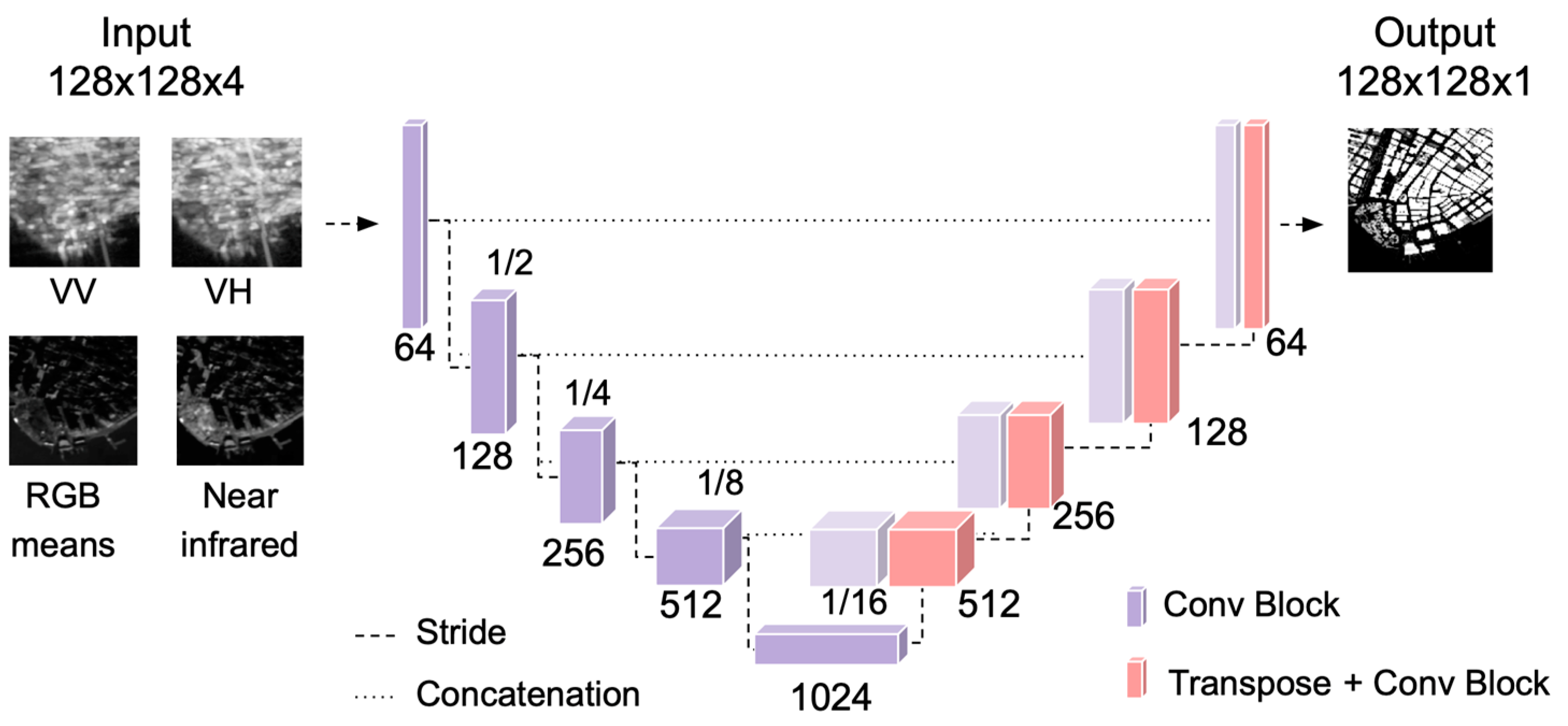
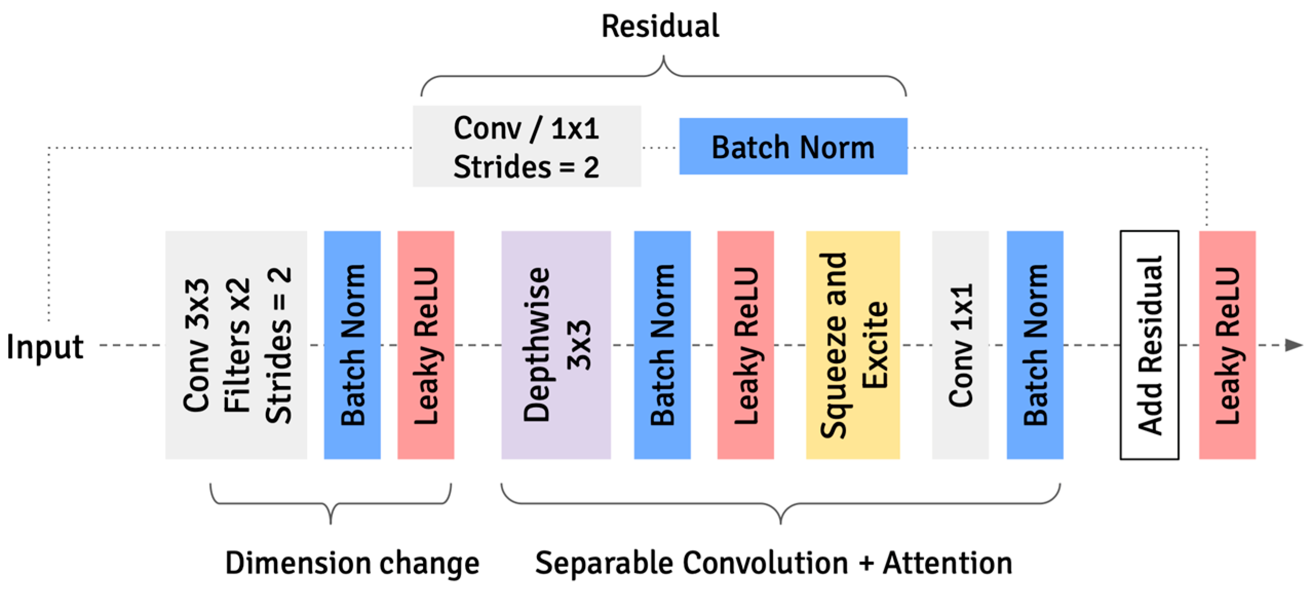
2.4. U-Net Architecture

U-Net, a fully convolutional network, was initially designed for biomedical image segmentation [17,26] which features a symmetric encoder–decoder structure along with skip connections to link corresponding layers between the encoder and decoders. The U-Net architecture is widely used in height estimation from satellite imagery, as proposed by Amirkolaee & Arefi [27] to be the most effective architecture for extracting height information from aerial optical imagery and applied in models such as IM2HEIGHT by Mou & Zhu [28], IM2ELEVATION by Liu et al. [29], and IMG2NDSM by Karatsiolis et al. [30]. Furthermore, studies mentioned in Section 1.2 utilize the modification of U-Net to extract and estimate surface height from SAR intensity imagery. In this study, we selected U-Net as the main model architecture as demonstrated by the success of the previous study. The U-Net model (Figure 2) in this study employs the use of strides to reduce the spatial dimensions within the encoder as well as transpose convolution to reconstruct the encoded information back to its original resolution in order to preserve spatial information and maintain learnable down/up sampling during the reconstruction process. A dropout of 0.3 is set at the end of each layer of the encoder and decoder intended to prevent overfitting and improve generalization during training.

The convolutional block in this study, applied in each layer of the encoder and decoder of the U-Net, is inspired by MobileNet v3 [31] (Figure 3), which incorporates depthwise separable convolution and the Squeeze-and-Excitation (SE) attention mechanisms [32]. The depthwise convolution processes spatial information independently across the expanded channels. The SE attention recalibrates channel-wise features to emphasize more important channels within the feature maps [32]. This attention differs from generative attention as it does not generate new representations but rather enhances it by reinforcing relevant features. The pointwise convolution is then applied to reduce the dimensionality back to the original number of channels, and the result is added to the residual connection, forming an inverted residual block. This structure of the convolutional block (Figure 3) is designed to reduce computational complexity while maintaining the strong representational capacity, thus enabling the efficient learning of spatial and contextual patterns in both SAR and optical images.

2.5. Hyperparameter, Loss Functions and Metrics

The hyperparameter of the model for both iterations was determined empirically through iterative refinement while adhering to the established deep learning practices for vision-based tasks. The selection of 20 epochs, a batch size of 16 image patches, and a decreasing learning rate with the cosine annealing method from 1 × 10⁻³ to 1× 10⁻⁴ is based on balancing convergence stability and generalization in inference performance. The model in both iterations was trained using a loss function that integrates both absolute height metrics with structural similarity to enhance reconstruction accuracy.

L1 Loss or the Mean Absolute Error (MAE) is selected as the main reconstruction loss function:

$$MAE={\displaystyle \frac{1}{n}}\sum |y_i-{\widehat{y}}_i|$$

(1)

where n is the number of pixels, $y_i$ is the true height, and ${\widehat{y}}_i$ is the predicted height in meters.

In addition, the Structural Similarity Index Measure (SSIM) is defined as:

$$SSIM={\displaystyle \frac{{(2\mu }_x{\mu }_y+C_1\left)\right(2{\sigma }_{xy}+C_2)}{\left({\mu }_x^2+{\mu }_y^2+C_1\right)\left({\sigma }_x^2+{\sigma }_y^2+C_2\right)}}$$

(2)

Here, ${\mu }_x$ and ${\mu }_y$ are the means of the two images, ${\sigma }_x^2$ and ${\sigma }_y^2$ are the variance, ${\sigma }_{xy}$ is the covariance, and $C_1$ and $C_2$ are constants defined as ${\left(K_{1}L\right)}^2$ and ${\left(K_{2}L\right)}^2$, where $K_1$ = 0.01, $K_2$ = 0.03, and L is the dynamic height range of the NDSM patch. The SSIM value ranges from 0 to 1, where 1 indicates identical structural similarity between reconstructed and true NDSM.

To evaluate the model, the following metrics are used in addition to MAE:

Root Mean Square Error (RMSE), defined as:

$$RMSE=\sqrt{({\displaystyle \frac{1}{n}}\sum {(y_i-{\widehat{y}}_i)}^2)}$$

(3)

and R², defined as:

$$R^2=1-{\displaystyle \frac{\sum {\left(y_i-{\widehat{y}}_i\right)}^2}{\sum {\left(y_i-\overline{y}\right)}^2}}$$

(4)

where R² of 1 represents perfect pixel-to-pixel fitting between height values of reconstructed and true NDSM.

These metrics provide robust absolute height errors as well as data fit between true and predicted NDSM. Furthermore, each of these metrics was calculated for pixels that belong to built and vegetation features. The separation of the two features was accomplished by calculating Enhance Vegetation Index (EVI) using the S2 Red, Blue, and NIR, defined as:

$$EVI={\displaystyle \frac{(NIR-Red)}{(NIR+Red{·C}_1-Blue{·C}_2+L)}}$$

(5)

where C₁ and C₂ represent atmospheric resistance and are set to 6 and 7.5, respectively, while L represents the adjustment for canopy noise and is set to 1. This parametric adjustment reduces noises and saturation, thus enhancing sensitivity to effectively distinguish vegetation to non-vegetation areas, as compared to other greenness indices such as the normalized difference vegetation index (NDVI) [33]. The classification scheme is performed by applying a threshold to the combination of EVI and height values from the true NDSM, defined as:

$$\begin{array}{l}Ground=NDSM<2\\ Built=NDSM>2 and EVI\le 0.05\\ Vegetation=NDSM>2 and EVI>0.05\end{array}$$

(6)

The separation of built and vegetation pixels allows for a comparative assessment of the quality of the fit and evaluates the model’s estimation performance across different land cover types.

3. Results

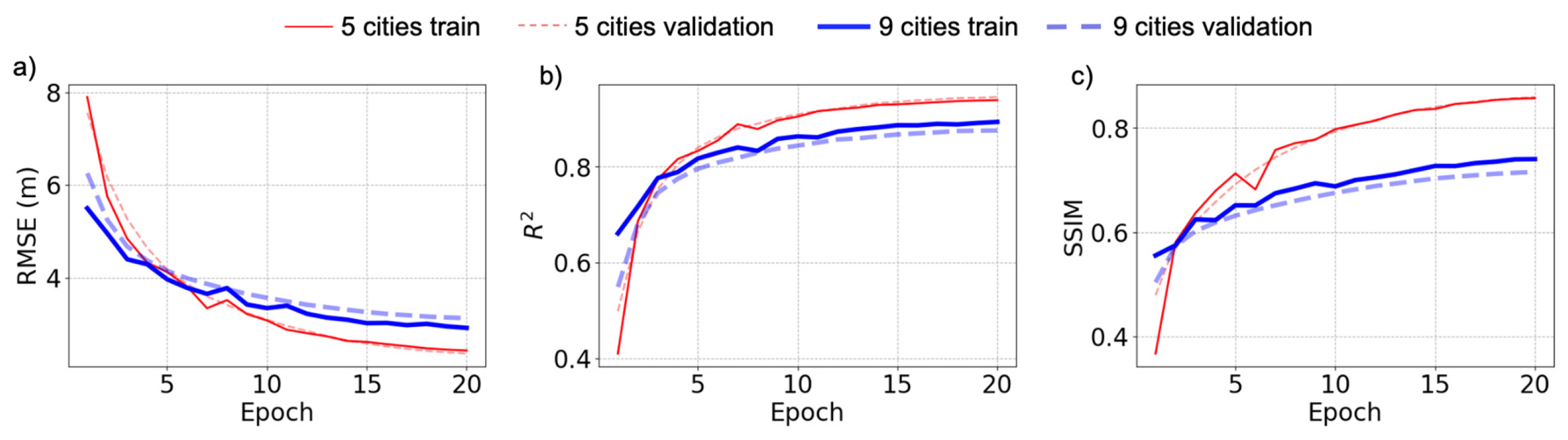
3.1. Training Performance

The metric curves from training performance demonstrate convergence between training and validations in both models (Figure 4). Overall, the two models exhibit consistent improvement across all metrics as training progresses. It is, however, important to note that the datasets for the models differ, as the dataset for the nine cities model includes the original five larger cities with an addition of four smaller cities and the city centers of each city in the data, and thus direct comparison is less straightforward but reflects different underlying distributions between the two datasets. Nevertheless, the model trained better on the smaller dataset, as the validation RMSE was lower (2.43 m) for the model trained on the five main cities compared to the validation RMSE (3.13 m) from the model trained on the five main cities with the additional four smaller cities and the five city centers. Similarly, the model trained on the smaller dataset had a higher SSIM of 0.85 as opposed to 0.74 from the nine-cities model. The R² values are closer between the two models, with the five-cities model slightly outperforming, suggesting that both achieve a similar level of fit to their respective datasets. This result suggests that the model trained on the smaller dataset with only five cities benefits from a more constrained feature space, leading to a lower RMSE and higher R² and SSIM, but potentially reduces generalization due to overfitting. In contrast, the inclusion of additional data from four cities and the different patches from the original five city centers increases feature diversity, improving the robustness of the model but also making optimization more challenging.

3.2. Inference Comparison on Test Dataset

The performance of the model’s inferences is evaluated by taking the overall average of each metric across all test cities to further quantify the predictive capability of the two models on images from the cities not included in the training process (

Table 1. Metrics for the U-Net model trained with the five main cities and nine cities, separated by built and vegetation pixels derived from EVI and NDSM thresholding.

Training Size	RMSE (m)	RMSE Built (m)	RMSE Veg (m)	MAE (m)	MAE Built (m)	MAE Veg (m)	R2	R2 Built	R2 Veg
5 Cities	10.84	16.08	11.47	5.86	10.51	6.97	0.54	0.45	0.21
9 Cities	10.22	14.99	10.38	5.28	9.41	6.24	0.58	0.52	0.32

). Overall, there is a noticeable improvement in inferences with the model trained on a larger collection of cities. Although overall RMSE, MAE, and R² of have only slightly improved, the inference performance of the model trained on more cities results in lower absolute metrics as well as better fitting, particularly for built and vegetation pixels. The nine-cities models have more than 1 m reduction on both RMSE and MAE for the built pixels as compared to the 5-cities models, suggesting that the model learns more from large collection of cities. Such reduction however is slightly less pronounced for vegetation but the significant gain in R² indicates that the addition of the cities allows the model to better capture of vegetation features from the input images.

When looking closer at a small region of interest as an example, a visual comparison between the outputs of the nine-cities model and the five-cities model shows enhancement in the overall features of the prediction as well as a smaller RMSE and MAE (Figure 5). The shapes of large buildings and urban clusters are more sharply defined, suggesting that the addition of cities and city centers augments the model’s capability to better capture the spatial structures and details in built environments. Such enhancement in visual clarity, particularly for large structures, indicates the model’s improved ability to generalize shapes and provide more accurate representations across different cityscapes.

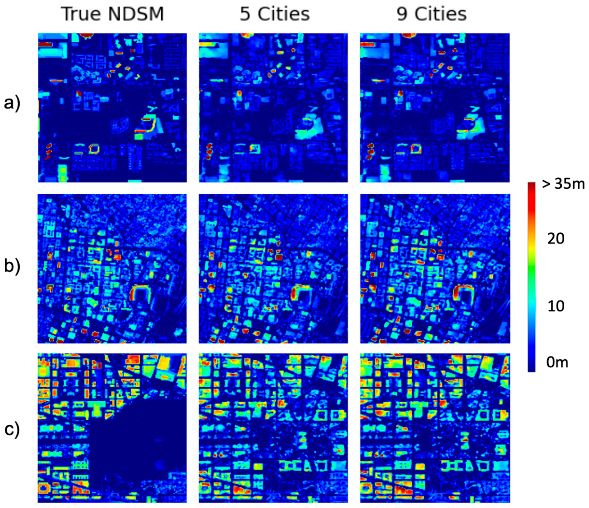
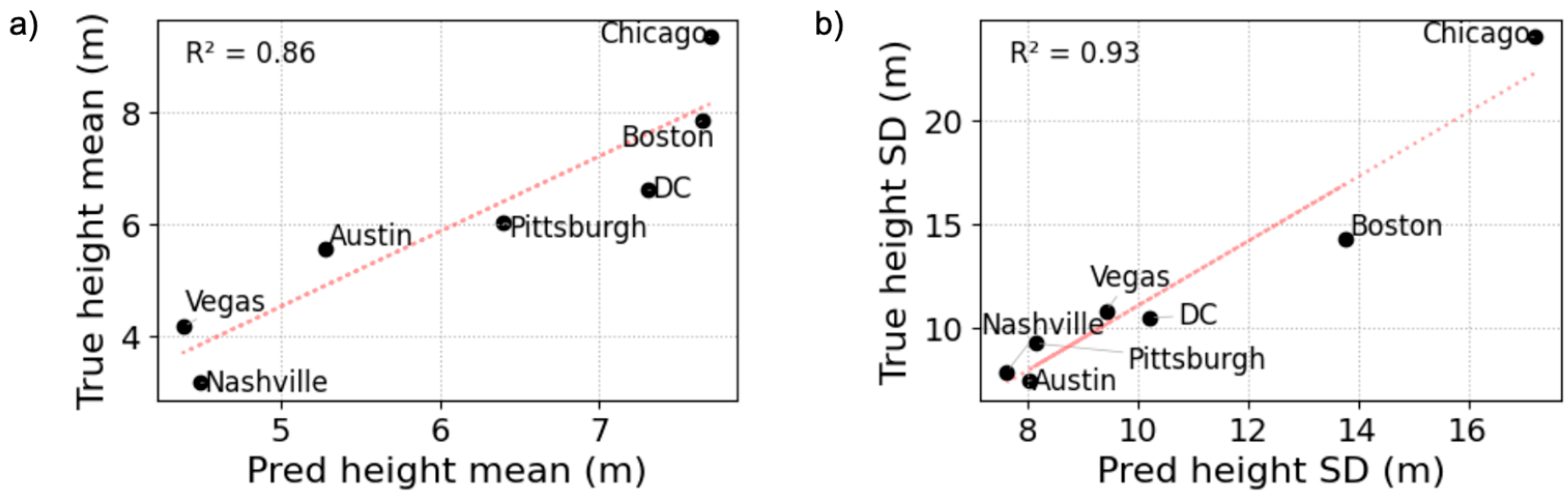
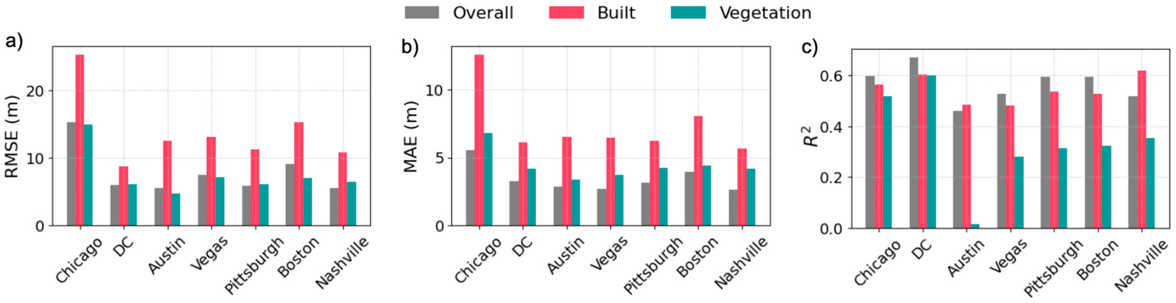
3.3. Height Estimation on Test Cities

Moving onwards, the model trained on nine cities with additional areas from the city centers will be used for further analysis due to its improved inference performance across absolute metrics and fitting as well as enhancement in capturing both built and vegetation features. The inferences for each city overall demonstrate a strong correlation between the mean heights and standard deviations (SD) of the predicted and true NDSM, with R² values of 0.86 and 0.94 respectively. The fit line on Figure 6 can be used to estimate bias in the inferences, where cities that lie above the fit line on Figure 6 indicate underestimation while cities below the line indicate overestimations. Chicago, which has the highest mean height, is the furthest above the line in both mean height and standard deviation, which suggests the challenge the model faces when dealing with such a complex city with height variation from skyscrapers and dense urban centers. The cases of Nashville and Washington DC, which exhibit slight underestimations, do not have a wide spread of height deviations and may indicate the influence of other underlying features of the input images that are not directly captured by the model.

To further analyze the inference performance of the model, the bar chart in Figure 7 compares the error metrics across different test cities and is separated by built and vegetation features. Overall, the RMSE and MAE for built features are consistently higher as compared to the overall and vegetation features. Taller cities such as Chicago and Boston are prime examples of high RMSE error, as these cities are globally known for their business centers that are densely populated with tall buildings. The rest of the test cities exhibit similar lower MAE values. When looking at the R² fit, the vegetation R² is generally lower than the R² for built features, particularly in Austin. Such low performance may suggest a potential limitation, as fine-grained vegetation features pose a challenge in which the model still struggles to capture effectively.

A direct comparison of our model’s performance with existing studies in 1.2 via overall height metrics performance is challenging, as height error in meters inherently depends on the specific height distribution of features in each of the study areas. For example, Cao and Weng [20] reported RMSE values that varied regionally from 4.11–10.32 m and MAE values of 2.59–6.09, to which we observed similar range in the overall height reconstruction of all features (RMSE ~ 4–15 m; MAE ~ 3–5 m). In contrast, R² provides a more uniform basis of fitness between true and predicted height values. Our model achieved overall R² ranging from slightly below 0.5 to 0.67, comparable to 0.61 R² reported by Nascetti et al. [19] for their model trained on cities in the Netherlands. However, it must be noted that the existing studies focus on the building height reconstruction, as opposed to ours where building and vegetation area are both included in the surface height reconstruction, increasing the complexity of the reconstruction. We further highlight the challenges associated with reconstructing correct building shapes in the discussion, which are identified as the key factors influencing accuracy and fitting errors.

4. Discussion

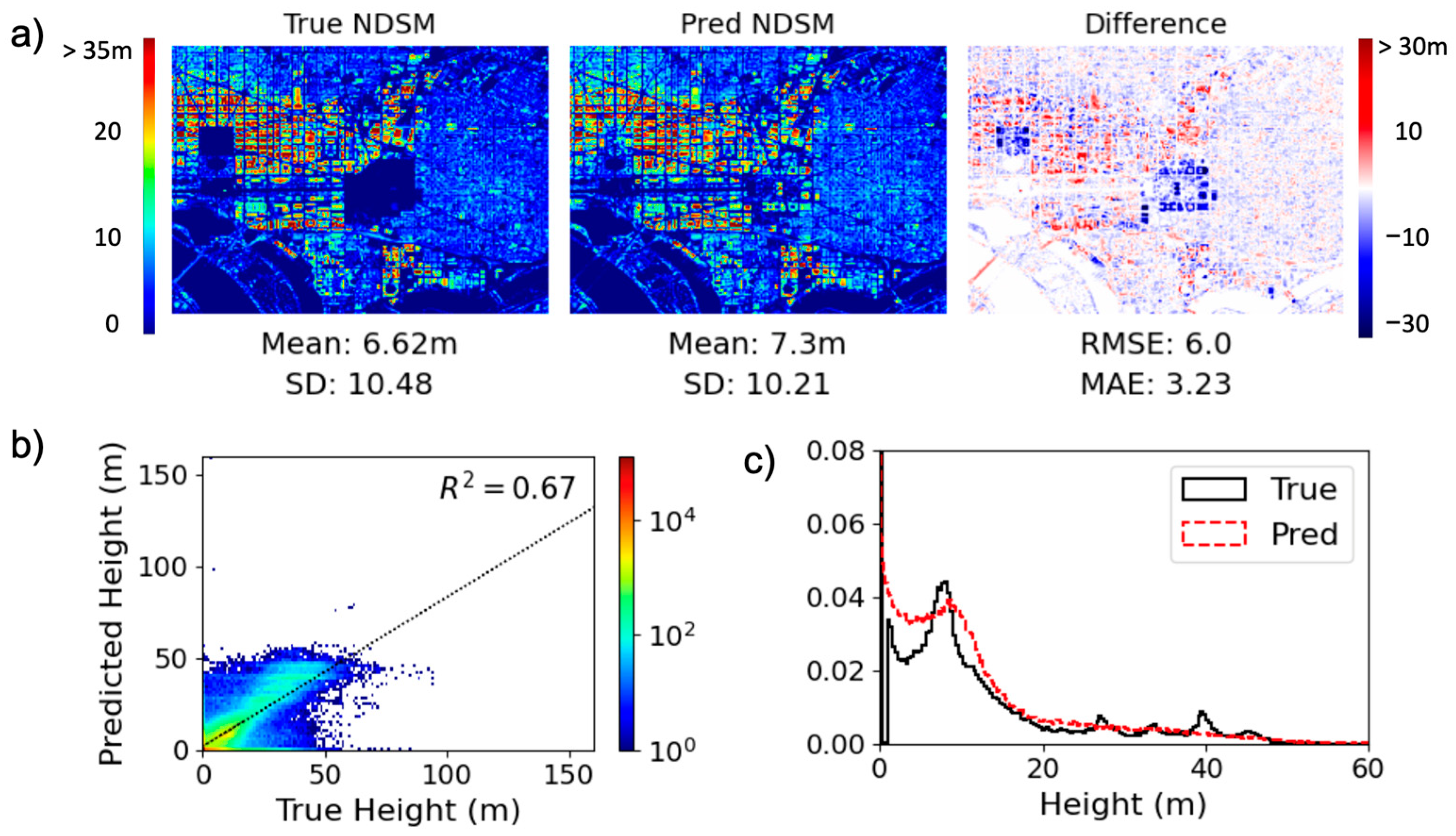
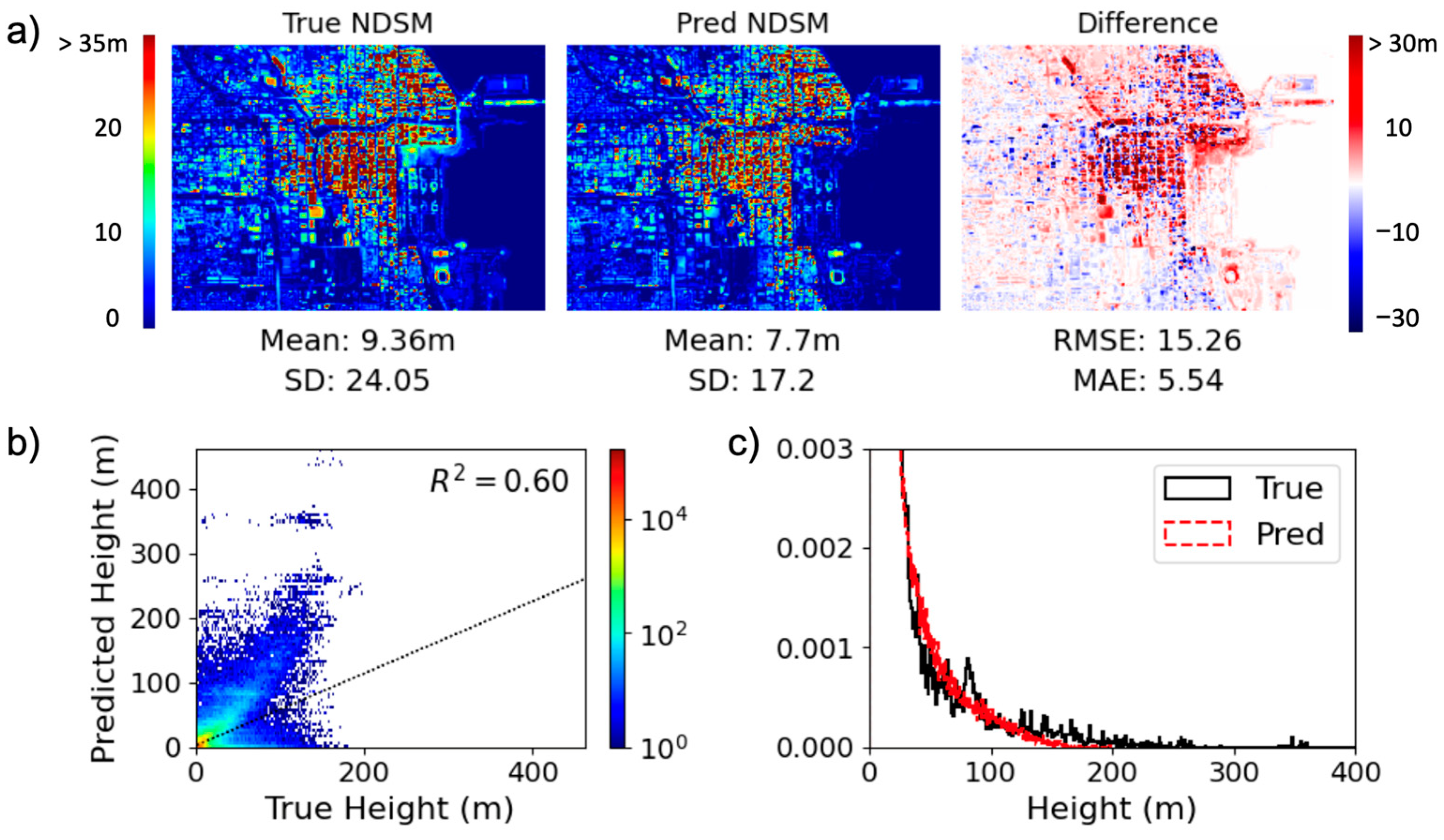
4.1. Comparative Study: Washington DC vs. Chicago

Results from the previous section indicate an estimation bias, with overestimations in Washington DC and underestimations in Chicago. While the latter city has a higher overall mean height, it is important to further analyze how the bias is distributed, spatially and across different height values. A detailed examination of such distributions will highlight the model’s limitation in extracting information and identify potation factors within the input sources contributing to the observed discrepancies.

The image differences in Figure 8 and Figure 9 are a result of subtracting the predicted NDSM from the true NDSM, where areas in red represent underestimation and areas in blue represent overestimation. In the case of Washington DC, the areas surrounding the city center appear predominantly blue, which indicates a tendency towards overestimations. The city centers, where taller buildings are located, tend to have patches of red, suggesting a localized underestimation. Noticeably, the big patches of blue shades in the center represent the missing government buildings, which are purposely left out for security reasons. Furthermore, there is a moderate fit between true and predicted heights, indicated by an R² of 0.67, but maintaining a large spread that funnels narrower as height increases. The height density distribution could offer a description to the observed funnel shape in the scatterplot. As shown in the density distribution plot, there is a noticeable gap between the true and predicted height distribution, with the predicted distribution being generally higher. Such an observation reinforces the overestimation seen in the blue areas surrounding the center as well as the larger spread in the lower height values between the true and predicted heights.

The difference image of Chicago (Figure 9), however, offers a contrasting picture compared to the difference image of Washington DC. Areas around the center are predominantly red and, as mentioned before, suggest height underestimation. There are small distributions of strong blue patches of overestimations within the central red areas. Moreover, the scatterplot between the true and predicted height shows a larger spread in the lower height values but sharply narrows as the height goes above 100 m. Interestingly, the predicted height distribution stops at around 200 m, to which the true height distribution stands above the predicted height distribution, creating a gap that represents underestimations of tall features. The contrasting distributions from Chicago to Washington DC highlight the model’s bias tendency, which is influenced by the complex urban features that the model struggles to capture effectively.

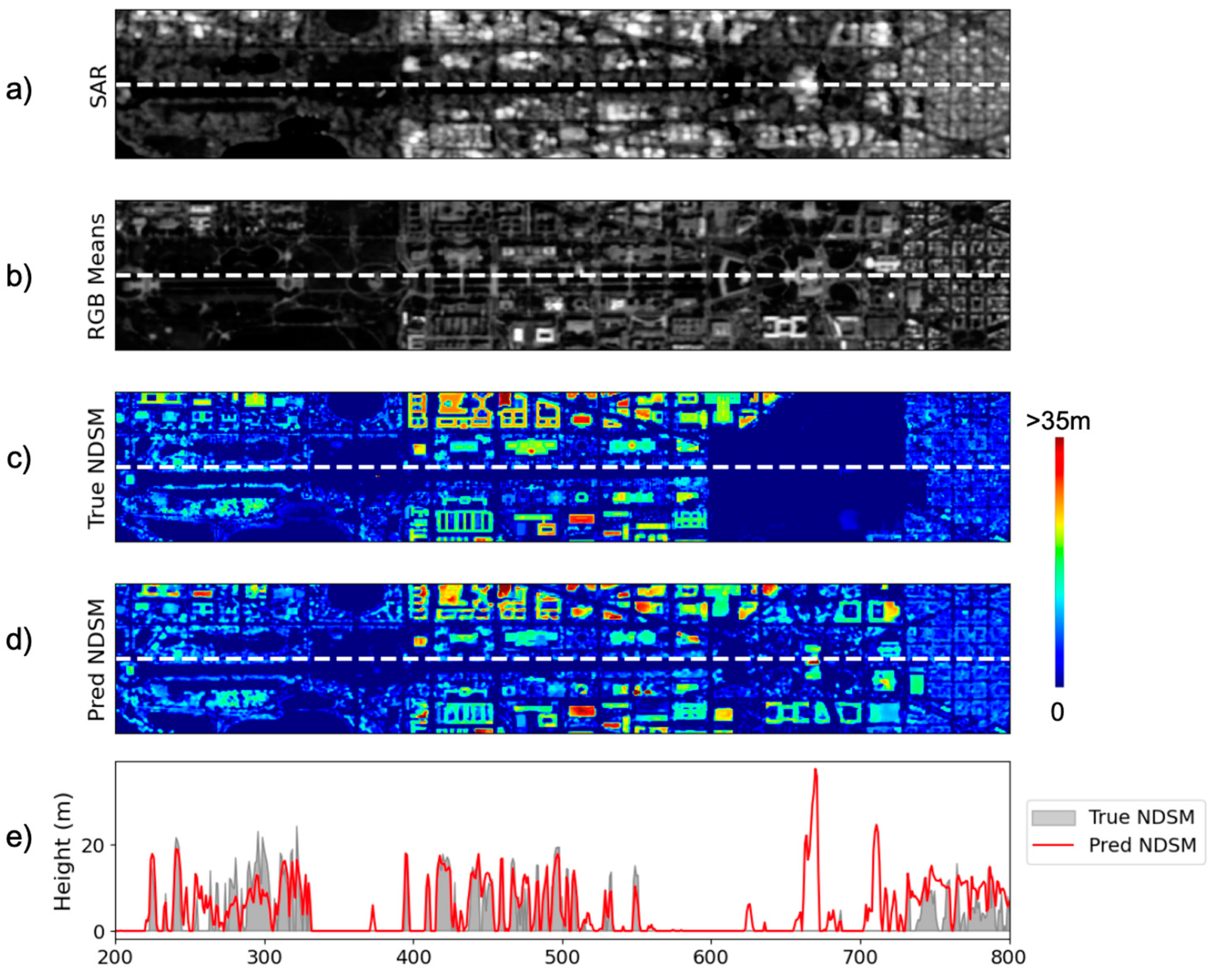
4.2. Cross-Section Analysis

Cross-section analysis between the true and predicted height was conducted with S1 SAR VH and S2 RGB means, as these two inputs offer a visually interpretable representation of all input data and balance structural and contextual details from SAR and optical images. The cross-section allows for a closer look at how the model’s height extraction functions by aligning the height profile spatially across the horizontal section of the city. Similarly to the previous section, cross-sections from Washington DC and Chicago centers are used to demonstrate the strengths and limitations of the model in capturing complex urban features.

The cross-section from Washington DC focuses on the National Mall, the heart of the city where key landmarks and governmental buildings are concentrated and therefore provides an ideal region to assess the model’s performance (Figure 10). Noticeably, areas within Capitol Hill boundary are exempted from the true NDSM for security concerns. The models, using the 4 input satellites images (2 shown), were able to fill in the missing buildings in the predicted NDSM. Furthermore, the shapes of the buildings, which may not be delineated clearly in the SAR and RGB means images, are effectively captured in the predicted NDSM and closely resemble the shapes in true NDSM. While the shapes of the buildings are conserved, the height does not distribute uniformly in many buildings, which results in underestimations. The overestimations are clearly shown towards the right end of the cross-section, a region where, although lower in height, are denser compared to the main central area of the image. Overall, the SAR image, with relatively low geometric distortion, combines effectively with the optical image, which enhances the model’s success, demonstrated by the preservation of building shapes in the predicted NDSM.

In the case of the cross-section from Chicago, although street canyons are well preserved, the buildings’ shapes in the predicted NDSM are less defined and deterred by height underestimation (Figure 11). Such an underestimation and lack of defined shape is particularly prominent in areas within the middle of the image, where tall buildings are densely concentrated. Contrastingly, the predicted shapes and heights are more aligned on outer regions where buildings are shorter. Such a disparity in model performance could be explained by geometric distortion in the SAR image. In the SAR image, the area in which underestimation occurs exhibits a loss of shapes and is dominated by bright layover pixels in the SAR image caused by multiple bounces of signals between buildings and the surrounding environments, which increases the intensity reading of the returning signal. This effect is amplified with greater building height and density, resulting in stronger geometric distortion. It is evident that these distortions in SAR intensity produce underestimation as the model failed to distil height information from the SAR image and correctly assign it to the building to which it belongs. The areas beside these regions have fewer layovers and are more similar to the case of Washington DC, where the model was able to effectively delineate buildings with less underestimation. This highlights the limitations of the model in dealing with complex urban environments, where signal distortions interfere with accurate height predictions. Addressing these challenges may require enhanced preprocessing techniques or alterations to the model architecture and convolution blocks better suited to handling SAR-specific artifacts.

4.3. Challenges and Paths to Model Improvement

There are two main challenges observed in this study:

• Overfitting: Although increasing the size and city variability of the training dataset improves the overall inference performance on the test dataset, the average RMSE (10.22 m) of the test set is much larger than the RMSE of the validation set (2.43 m). Similarly, the average R² for the test set is well below the validation R². While the cross-section provides valuable insights and demonstrates certain strengths, there remains a need to address the estimation bias to achieve generalization and more accurate results.
  To improve the model’s performance and reduce overfitting, there is a need for a refined approach to data curation as different cities possess unique complexity. Such curation could involve a study focusing on creating a better-balanced dataset based on machine learning clustering analysis that accurately characterizes the diverse height distribution of the urban features, relating to how they are represented in the input satellite imagery. Additionally, alternative training methods such as ensemble learning utilizing k-fold cross-validation could be explored to enhance the robustness of the model. Other potential strategies, such as the incorporation of multi-task learning, as in the approach by Cai et al. where the model outputs both building heights and footprints, could leverage the model’s mechanism in alleviating biases and enhance the capability of generalizing across varying urban landscapes.
• SAR artifacts: The model inference performs poorly on areas with heavy geometric distortion where the SAR intensity image is dominated with layovers. In the case of Chicago, the layover from the densely populated tall buildings spills onto the surrounding areas. Such distortion expectedly creates a significant challenge for the model to extract surface height information and maintain fine shapes of features.
  Applying CNN to a geometrically distorted image is always a challenge. Recla & Schmitt [12] introduced a preprocessing method that projected true NDSM for training onto the SAR coordinate system, with an addition of parameter injection into the model to improve the overall estimation. The performance of the model, however, still possesses drawbacks in denser areas with tall buildings, where individual buildings’ layovers are indistinguishable from one another. The option to create aggregate intensity at larger resolutions, such as the approach applied by Li et al. [15] may not be suitable for urban applications as it significantly reduces the resolution of the image. This challenge leads to the need for expanding the understanding of the convolutions and their corresponding weights. Techniques from explainable AI can offer deeper insights into the relationship between the input satellite imagery and the generated NDSM, therefore providing a clearer interpretation of the underlying mechanism which can be leveraged to produce a more effective convolutional block that fully captures the height information.

5. Conclusions

This study examines the potential of deep learning to extract height information from open-source Sentinel 1 (radar) and Sentinel 2 (multispectral) imagery to produce a normalized digital surface model for urban areas. Two training iterations were performed using MobileNet v3-inspired U-Net and trained on different datasets consisting of the five largest cities in the United States and an addition of four smaller cities. The test set for inference includes a range of cities with varying height means and deviations. The addition of smaller cities shows an improvement in the model’s inference, demonstrated by lower average RMSE and MAE as well as higher R². While the test inference metrics from the test sets show promises, a comparison of the inference performance for validation with the test dataset shows overfitting. Further analysis using difference calculations, height distribution, and cross-sectional studies suggest that areas with estimation bias are influenced by the image resolution as well geometric distortions from the SAR image. An improvement on the model requires the refinement of data curation and the employment of advanced training techniques. Furthermore, integrating explainable AI techniques can be applied to gain insights into the underlying mechanisms of the model that will be useful in enhancing the convolutional blocks to better capture height information.

References

1. Braun, A. Retrieval of Digital Elevation Models from Sentinel-1 Radar Data—Open Applications, Techniques, and Limitations. Open Geosci. 2021, 13, 532–569. [Google Scholar] [CrossRef]
2. Soergel, U. (Ed.) Radar Remote Sensing of Urban Areas; Remote Sensing and Digital Image Processing; Springer Netherlands: Dordrecht, The Netherlands, 2010; Volume 15, ISBN 978-90-481-3750-3. [Google Scholar]
3. Thiele, A.; Wurth, M.M.; Even, M.; Hinz, S. Extraction of Builidng Shape from Tandem-X Data. Int. Arch. Photogramm. Remote Sens. Spat. Inf. Sci. 2013, XL-1/W1, 345–350. [Google Scholar] [CrossRef]
4. Koppel, K.; Zalite, K.; Voormansik, K.; Jagdhuber, T. Sensitivity of Sentinel-1 Backscatter to Characteristics of Buildings. Int. J. Remote Sens. 2017, 38, 6298–6318. [Google Scholar] [CrossRef]
5. Rodríguez, E.; Morris, C.S.; Belz, J.E. A Global Assessment of the SRTM Performance. Photogramm. Eng Remote Sens. 2006, 72, 249–260. [Google Scholar] [CrossRef]
6. Misra, P.; Avtar, R.; Takeuchi, W. Comparison of Digital Building Height Models Extracted from AW3D, TanDEM-X, ASTER, and SRTM Digital Surface Models over Yangon City. Remote Sens. 2018, 10, 2008. [Google Scholar] [CrossRef]
7. Uuemaa, E.; Ahi, S.; Montibeller, B.; Muru, M.; Kmoch, A. Vertical Accuracy of Freely Available Global Digital Elevation Models (ASTER, AW3D30, MERIT, TanDEM-X, SRTM, and NASADEM. Remote Sens. 2020, 12, 3482. [Google Scholar] [CrossRef]
8. Gross, K.; Corseaux, A. Copernicus DEMs Quality Assessment Summary; European Space Agency (ESA): Paris, France; Telespazio: Rome, Italy, 2021.
9. Copernicus Data Space Ecosystem. Copernicus Copernicus DEM—Global and European Digital Elevation Model. Available online: https://dataspace.copernicus.eu/explore-data/data-collections/copernicus-contributing-missions/collections-description/COP-DEM (accessed on 30 July 2024).
10. Rossi, C.; Gernhardt, S. Urban DEM Generation, Analysis and Enhancements Using TanDEM-X. ISPRS J. Photogramm. Remote Sens. 2013, 85, 120–131. [Google Scholar] [CrossRef]
11. Sun, Y.; Montazeri, S.; Wang, Y.; Zhu, X.X. Automatic Registration of a Single SAR Image and GIS Building Footprints in a Large-Scale Urban Area. ISPRS J. Photogramm. Remote Sens. 2020, 170, 1–14. [Google Scholar] [CrossRef] [PubMed]
12. Recla, M.; Schmitt, M. Deep-Learning-Based Single-Image Height Reconstruction from Very-High-Resolution SAR Intensity Data. ISPRS J. Photogramm. Remote Sens. 2022, 183, 496–509. [Google Scholar] [CrossRef]
13. Shi, C.; Zuo, X.; Zhang, J.; Zhu, D.; Li, Y.; Bu, J. Accuracy Assessment of Geometric-Distortion Identification Methods for Sentinel-1 Synthetic Aperture Radar Imagery in Highland Mountainous Regions. Sensors 2024, 24, 2834. [Google Scholar] [CrossRef] [PubMed]
14. Tao, J.; Palubinskas, G.; Reinartz, P.; Auer, S. Interpretation of SAR Images in Urban Areas Using Simulated Optical and Radar Images. In Proceedings of the 2011 Joint Urban Remote Sensing Event, Munich, Germany, 11–13 April 2011; pp. 41–44. [Google Scholar]
15. Li, X.; Zhou, Y.; Gong, P.; Seto, K.C.; Clinton, N. Developing a Method to Estimate Building Height from Sentinel-1 Data. Remote Sens. Environ. 2020, 240, 111705. [Google Scholar] [CrossRef]
16. Frantz, D.; Schug, F.; Okujeni, A.; Navacchi, C.; Wagner, W.; van der Linden, S.; Hostert, P. National-Scale Mapping of Building Height Using Sentinel-1 and Sentinel-2 Time Series. Remote Sens. Environ. 2021, 252, 112128. [Google Scholar] [CrossRef] [PubMed]
17. Ronneberger, O.; Fischer, P.; Brox, T. U-Net: Convolutional Networks for Biomedical Image Segmentation. In Medical Image Computing and Computer-Assisted Intervention—MICCAI 2015: 18th International Conference; Springer International Publishing: Cham, Switzerland, 2015; pp. 234–241. [Google Scholar]
18. Cai, B.; Shao, Z.; Huang, X.; Zhou, X.; Fang, S. Deep Learning-Based Building Height Mapping Using Sentinel-1 and Sentienl-2 Data. Int. J. Appl. Earth Obs. Geoinf. 2023, 122, 103399. [Google Scholar]
19. Nascetti, A.; Yadav, R.; Ban, Y. A CNN Regression Model to Estimate Buildings Height Maps Using Sentinel-1 SAR and Sentinel-2 MSI Time Series. In Proceedings of the IGARSS 2023-2023 IEEE International Geoscience and Remote Sensing Symposium, Pasadena, CA, USA, 16–21 July 2023; pp. 2831–2834. [Google Scholar]
20. Cao, Y.; Weng, Q. A Deep Learning-Based Super-Resolution Method for Building Height Estimation at 2.5 m Spatial Resolution in the Northern Hemisphere. Remote Sens. Environ. 2024, 310, 114241. [Google Scholar] [CrossRef]
21. European Space Agency Sentinel-1: ESA’s Radar Observatory Mission for GMES Operational Services 2013. Available online: https://esamultimedia.esa.int/docs/S1-Data_Sheet.pdf (accessed on 30 November 2024).
22. European Space Agency Sentinel-2: Optical High-Resolution Mission for GMES Operational Services 2013. Available online: https://esamultimedia.esa.int/docs/S2-Data_Sheet.pdf (accessed on 30 November 2024).
23. U.S. Geological Survey. LiDAR Point Cloud Data for Various U.S. Cities. 2017–2022. Available online: https://apps.nationalmap.gov/downloader/ (accessed on 30 May 2024).
24. New York City Department of Environmental Protection. NYC LiDAR 2017 Dataset. 2017. Available online: https://data.cityofnewyork.us (accessed on 30 May 2024).
25. District of Columbia Government. DC LiDAR 2022 Dataset. 2022. Available online: https://opendata.dc.gov (accessed on 30 May 2024).
26. Siddique, N.; Paheding, S.; Elkin, C.P.; Devabhaktuni, V. U-Net and Its Variants for Medical Image Segmentation: A Review of Theory and Applications. IEEE Access 2021, 9, 82031–82057. [Google Scholar] [CrossRef]
27. Amirkolaee, H.A.; Arefi, H. Height Estimation from Single Aerial Images Using a Deep Convolutional Encoder-Decoder Network. ISPRS J. Photogramm. Remote Sens. 2019, 149, 50–66. [Google Scholar]
28. Mou, L.; Zhu, X.X. IM2HEIGHT: Height Estimation from Single Monocular Imagery via Fully Residual Convolutional-Deconvolutional Network 2018. arXiv 2018, arXiv:1802.10249. [Google Scholar]
29. Liu, C.J.; Krylov, V.A.; Kane, P.; Kavanagh, G.; Dahyot, R. IM2ELEVATION: Building Height Estimation from Single-View Aerial Imagery. Remote Sens. 2020, 12, 2719. [Google Scholar] [CrossRef]
30. Karatsiolis, S.; Kamilaris, A.; Cole, I. IMG2NDSM: Height Estimation from Single Airborne Rgb Images with Deep Learning. Remote Sens. 2021, 13, 2417. [Google Scholar] [CrossRef]
31. Howard, A.; Sandler, M.; Chu, G.; Chen, L.C.; Chen, B.; Tan, M.; Wang, W.; Zhu, Y.; Pang, R.; Vasudevan, V.; et al. Searching for MobileNetV3. In Proceedings of the IEEE International Conference on Computer Vision (ICCV), Seoul, Republic of Korea, 27 October–2 November 2019; pp. 2559–2567. [Google Scholar]
32. Hu, J.; Shen, L.; Sun, G. Squeeze-and-Excitation Networks. In Proceedings of the IEEE Conference on Computer Vision and Pattern Recognition, Salt Lake City, UT, USA, 18–22 June 2018; pp. 7132–7141. [Google Scholar]
33. Huete, A.; Didan, K.; Miura, T.; Rodriguez, E.P.; Gao, X.; Ferreira, L.G. Overview of the Radiometric and Biophysical Performance of the MODIS Vegetation Indices. Remote Sens. Environ. 2002, 83, 195–213. [Google Scholar] [CrossRef]
Figure 1. Cities used in training datasets: five main cities in red and four additional cities in blue. Cities in black are part of the test set and used for inference.
Remotesensing 17 01297 g001
Figure 2. U-Net Architecture with four input channels (VV, VH, RGB means, and Near Infrared) with skip connections between each layer in the encoder and decoder. The output is a 1 channel NDSM.
Remotesensing 17 01297 g002
Figure 3. Convolutional residual block used in each layer of U-Net (Figure 2) with dimensionality transformation, filter expansion, and separable depthwise convolution with Squeeze and Excite attention mechanism.
Remotesensing 17 01297 g003
Figure 4. RMSE (a), R2 (b), and SSIM (c) training (solid) and validation (dashed) performance for 20 epochs. It must be noted that the model with nine (blue) cities has a larger dataset than the model trained with only the five main cities (red).
Remotesensing 17 01297 g004
Figure 5. Visual comparison of predicted NDSM sample regions from test cities Las Vegas (a), Austin (b), and Washington DC (c), generated from the models trained with five cities and nine cities. Building shapes in the predicted NDSM from the nine-cities model are more defined.
Remotesensing 17 01297 g005
Figure 6. Scatterplots of the comparison between predicted and true height mean (a) and predicted and true height standard deviation (b) for test cities.
Remotesensing 17 01297 g006
Figure 7. Bar charts showing RMSE (a), MAE (b), and (c) for overall, built, and vegetation areas across test cities.
Remotesensing 17 01297 g007
Figure 8. Comparison for Washington DC: true and predicted NDSM, and their difference with (a) true and predicted height scatterplot (b) and histograms (c).
Remotesensing 17 01297 g008
Figure 9. True NDSM compared to predicted NDSM and their difference for Chicago with (a) true and predicted height scatterplot (b) and histograms (c).
Remotesensing 17 01297 g009
Figure 10. Cross-section of the National Mall in Washington DC with missing Capitol Hill area in true NDSM. Height profile (e) is represented by the white dashed lines on the SAR VH (a) RGB means (b), true (c) and predicted (d) NDSM images. Only two inputs out of 4 are shown for contextual and visual interpretability.
Remotesensing 17 01297 g010
Figure 11. Cross section of Downtown Chicago. Height profile (e) represents the white dashed lines on the SAR VH (a), RGB means, and (b) true and (c) predicted (d) NDSM images. Only two inputs out of 4 are shown for contextual and visual interpretability.
Remotesensing 17 01297 g011