Multi-Dimensional Parameter-Estimation Method for a Spatial Target Based on the Micro-Range Decomposition of a High-Resolution Range Profile

Abstract

The high-precision estimation of multi-dimensional parameters for spatial targets based on high-resolution range profiles is crucial for target recognition. However, existing estimation methods face difficulties in resolving the strong coupling between the target shape and the micro-motion parameters, as well as in fully utilizing micro-motion information under complex modulation characteristics. To address these challenges, this paper proposes a multi-dimensional parameter-estimation method for spatial targets based on micro-range decomposition. A micro-range model of the target is first constructed, and the micro-range modulation characteristics are analyzed. Then, micro-range coefficients are selected based on their Cramér–Rao lower bound (CRLB), and the correlation between these coefficients and target parameters is exploited for scattering center matching. An optimization model is further built for multi-dimensional parameter estimation, enabling the accurate estimation of parameters such as precession frequency, precession angle, and structural dimensions under both single-view and multi-view conditions. The experimental results show that in the dual-view case, all parameters are estimated with relative errors (REs) below 1.15% and root mean square error (RMSE) values below 0.05. In the single-view case, key parameters are estimated with REs under 15%. Compared with conventional methods, the proposed method achieves lower RMSE and significantly improved robustness and stability. These results demonstrate the effectiveness and practical potential of the proposed method for spatial target parameter estimation.

1. Introduction

The micro-motion of a space precession target induces complex micro-Doppler modulation characteristics in the radar echo, known as the micro-Doppler effect [1]. This effect encapsulates information regarding target shape, size, and scattering characteristics. Estimating these fine features of the target using high-resolution range profiles (HRRP) modulated by these complex characteristics is crucial for enhancing target recognition capability.

The electromagnetic scattering characteristics of space micro-moving targets serve as the foundation for acquiring micro-motion characteristics. Gao et al. established a relatively comprehensive micro-motion model for spatial targets, encompassing precession, nutation, and swing, and derived the micro-Doppler expressions resulting from these three micro-motions [2]. References [3,4] demonstrated through electromagnetic calculation simulations and experimental measurements that the scattering center of a space cone target consists of both the local scattering center and the sliding scattering center generated by edge diffraction.

With the advancement of electronic technology, radar systems operating at higher frequency bands and possessing larger bandwidths have opened up possibilities for extracting multi-dimensional fine features of spatial targets. These multi-dimensional parameters mainly include geometric structural features—such as the height of the cone body and the radius of its base—as well as micro-motion parameters, including precession frequency and precession angle. The authors of [5] utilized an improved CLEAN algorithm in conjunction with the phase information of HRRP to estimate the perturbation curve parameters of each scattering center, thereby achieving high-precision perturbation curve estimation. Reference [6] devised a method for estimating micro-motion periods based on the correlation of the time range distribution matrix, which is constructed from the observed HRRP sequence. Reference [7] employed independent component analysis for signal decomposition and data association in distributed radar networks, facilitating the estimation of micro-motion parameters and geometric structure parameters. Additionally, References [8,9,10] delved into the challenge of multidimensional parameter estimation under nutation and intermittent observation.

Most of these methods are based on the range change curve of the scattering center [11]. First, they assume that the micro-range projection change of the scattering center on the radar line of sight follows cosine modulation with bias, which differs from the actual scenario. Second, it is generally assumed that the micro-range curves of known scattering centers are attributed by default, lacking a matching and correlation method for scattering centers. In fact, the attribution of scattering centers is crucial for parameter estimation. Lastly, these methods fail to fully utilize the information provided by radar echoes. Single-view observation relies on prior information about the sight angle.

In response to the challenges posed by existing multi-dimensional parameter estimation algorithms, this paper presents a novel method for estimating multi-dimensional parameters of spatial targets based on the micro-range decomposition of HRRP. Initially, the micro-motion modulation characteristics of spatial targets are scrutinized through micro-range decomposition, and the the Cramér–Rao lower bounds (CRLBs) for estimating micro-rangeic coefficients are derived. These coefficients are then selected for parameter estimation. By leveraging the relationship between micro-range coefficients of each scattering center under different occlusion conditions, the matching correlation of the scattering centers is achieved. The super-resolution algorithm SRI-ESPRIT and the least squares method are utilized to estimate the micro-range coefficients, leading to the construction of a multi-dimensional parameter estimation optimization model, which is subsequently solved. Finally, the effectiveness of the proposed algorithm is verified using electromagnetic calculation data.

The structure of this article is organized as follows: Section 2 introduces the spatial target echo and micro-range model; Section 3 is based on SRI-ESPRIT and the minimum realized micro-range coefficient estimation; Section 4 proposes the scattering center matching correlation and spatial target multidimensional parameter estimation method; and Section 5 verifies the effectiveness of the algorithm proposed in this article through electromagnetic calculation data. Figure 1 clearly illustrates the overall algorithm pipeline, from micro-range decomposition to parameter optimization.

2. Modeling of Spatial Target Echoes and Motion

In this section, we will develop the radar echo model and micro-motion model for spatial targets to provide the necessary data support for the multi-dimensional parameter estimation method.

2.1. Modeling Echoes from Spatial Target

Assuming that each radar in the distributed radar system emits wideband linear frequency modulated (LFM) signals, and to prevent electromagnetic interference, each radar operates within a different frequency band. The transmitted signal for a particular sub-radar in the distributed radar network can be expressed as follows:

$$s\left(t_r,t_a\right)=rect\left({\displaystyle \frac{t_r}{T_p}}\right)\exp \left\{j2\pi \left(f_{c}t+{\displaystyle \frac{K_r{t_r}^2}{2}}\right)\right\},$$

(1)

where $T_p$, $K_r$, $f_c$, and $t_r=t-t_a$ represent the pulse width, chirp rate, carrier frequency, and fast time, respectively. Here, $K_r=B/T_p$, where B denotes the signal bandwidth. The variable t represents the total time, and $t_a$ represents the slow time. Additionally, $rect(·)$ denotes the rectangular window function.

Let us represent the range from a specific scatter center to the radar as $r_t$. Then, the radar echo from the target can be expressed as

$$s_r\left(t_r,t_a\right)=\sigma rect\left({\displaystyle \frac{t_r-\tau }{T_p}}\right)\exp \left\{j2\pi \left(f_c\left(t-\tau \right)+{\displaystyle \frac{1}{2}}{K}_r{\left(t_r-\tau \right)}^2\right)\right\},$$

(2)

where $\sigma$ denotes the radar cross-section (RCS), $\tau =2r_t/c$, and c represents the speed of light.

Assuming the range of the reference center is $r_{\mathrm{ref}}$, and ${\tau }_{\mathrm{ref}}=2r_{\mathrm{ref}}/c$, the reference signal is given by

$$s_{ref}\left(t_r,t_a\right)=\mathrm{rect}\left({\displaystyle \frac{t_r-{\tau }_{ref}}{T_{ref}}}\right)\exp \left\{j2\pi \left(f_c\left(t-{\tau }_{ref}\right)+{\displaystyle \frac{1}{2}}{K}_r{\left(t_r-{\tau }_{ref}\right)}^2\right)\right\},$$

(3)

where $T_{\mathrm{ref}}$ represents the pulse width of the reference signal.

After dechirping the radar echo using the reference signal, the resulting intermediate frequency (IF) signal is given by

$$\begin{array}{cc}\hfill s_{if}(t_a,t_r)& =s_r\left(t_a,t_r\right)\times s_{ref}^{*}\left(t_a,t_r\right)\hfill \end{array}$$

(4)

$$\begin{array}{cc}\hfill & =\mathrm{rect}\left({\displaystyle \frac{t_r-\tau }{T_r}}\right)\exp \left[-j{\displaystyle \frac{4\pi f_c}{c}}\left(r_t-r_{ref}\right)\right]\hfill \end{array}$$

(5)

$$\begin{array}{cc}\hfill & \times \exp \left[-j{\displaystyle \frac{4\pi }{c}}{K}_r\left(t_r-{\tau }_{ref}\right)\left(r_t-r_{ref}\right)\right]\exp \left[j{\displaystyle \frac{4\pi }{c^2}}{K}_r{\left(r_t-r_{ref}\right)}^2\right].\hfill \end{array}$$

(6)

Taking the Fourier transform of the IF signal with respect to the fast time, we obtain the frequency-domain signal:

$$\begin{array}{cc}\hfill S_{if}\left(t_a,f_r\right)& =T_r\sin c\left[T_r\left(f_r+K_r{\displaystyle \frac{2\left(r_t-r_{ref}\right)}{c}}\right)\right]\exp \left[-j{\displaystyle \frac{4\pi f_c}{c}}\left(r_t-r_{ref}\right)\right]\hfill \end{array}$$

(7)

$$\begin{array}{cc}\hfill & \times \exp \left[-j{\displaystyle \frac{4\pi f_r}{c}}\left(r_t-r_{ref}\right)\right]\exp \left[-j{\displaystyle \frac{4\pi }{c^2}}{K}_r{\left(r_t-r_{ref}\right)}^2\right],\hfill \end{array}$$

(8)

where $f_r$ represents the range frequency. Considering the frequency-domain signal as a narrow pulse with its peak occurring at $f_r=-2K_r\left(r_t-r_{\mathrm{ref}}\right)/c$, the residual video phase (RVP) can be approximated as

$${\displaystyle \Delta \phi =-\frac{4\pi f_r}{c}\left(r_t-r_{ref}\right)-\frac{4\pi }{c^2}{K}_r{\left(r_t-r_{ref}\right)}^2=\frac{\pi f_r^2}{K_r}.}$$

(9)

We obtain the phase compensation function as

$${\displaystyle H_{RVP}\left(f_r\right)=\exp (-j\Delta \phi )=\exp (-j\frac{\pi f_r^2}{K_r}).}$$

(10)

The pulse compression result is obtained as follows:

$$\begin{array}{cc}\hfill s_{out}& =S_{if}(t_a,f_r)\times H_{RVP}\left(f_r\right)\hfill \end{array}$$

(11)

$$\begin{array}{cc}\hfill & =T_r\sin c\left[T_r\left(f_r+K_r{\displaystyle \frac{2\left(r_t-r_{ref}\right)}{c}}\right)\right]\exp \left[-j{\displaystyle \frac{4\pi f_c}{c}}\left(r_t-r_{ref}\right)\right].\hfill \end{array}$$

(12)

2.2. Micro-Range Model of the Spatial Target

Establish a spatial cone target precession model as depicted in Figure 2, which includes a local ideal scattering center A, as well as sliding scattering centers B and C resulting from edge diffraction. For cone–cylinder targets, the primary difference lies only in the number of sliding scattering centers, which is not considered in this study. r and h correspond to the radius of the cone target’s base and the range from the cone’s centroid to the center of the base o, respectively, and H represents the height of the target’s main body. The initial range between the radar and the center of mass O is $r_0$. A local coordinate system $\left(x,y,z\right)$ is defined with o as the origin, and the axis of symmetry pointing toward the direction of the cone apex is designated as the z-axis. This axis remains stationary relative to the target. Additionally, a reference coordinate system $\left(X,Y,Z\right)$ is established with the reentry direction as the positive Z-axis. This coordinate system moves with the target while maintaining a static attitude with respect to the radar. During operation, the target spins around its local symmetry axis ($oz$) while simultaneously precessing around the reference axis ($OZ$). The rotation frequency about the $OZ$ axis is referred to as the precession frequency f, and the angle formed between the target’s spin axis ($oz$) and the precession axis ($OZ$) is denoted as the precession angle $\theta$. The angle between the radar line-of-sight and the target’s spin axis is defined as the aspect angle ${\gamma }_i$.

The angle between the projection of the radar line-of-sight direction onto the $XOY$ plane and the positive X-axis is calculated as shown in Equation (13), following the method described in [3].

$$\beta \left(t\right)=\mathrm{acos}(\cos {\gamma }_i\cos \theta +\sin {\gamma }_i\sin \theta \cos \left(2\pi ft+{\varphi }_0\right)),$$

(13)

where ${\varphi }_0$ denotes the initial phase.

Considering the cone top scattering center as the ideal scatter center and the scatter at the base of the cone as the sliding-type scatter center, let $a=\cos \theta \cos \gamma$, $b=\sin \theta \sin \gamma$ and $x\left(t\right)=\cos (2\pi ft+{\varphi }_0)$. During the target’s precession process, based on the geometric relationship of scatter centers, the radial ranges between each scatter center and the radar are, respectively, given by:

$$\begin{array}{cc}\hfill & r_A\left(t\right)=r_0-(H-h)(a+bx\left(t\right)),\hfill \end{array}$$

(14)

$$\begin{array}{cc}\hfill & {\displaystyle r_B\left(t\right)=r_0-r\sqrt{1-{\left(a+bx\left(t\right)\right)}^2}+h(a+bx\left(t\right)),}\hfill \end{array}$$

(15)

$$\begin{array}{cc}\hfill & {\displaystyle r_C\left(t\right)=r_0+r\sqrt{1-{\left(a+bx\left(t\right)\right)}^2}+h(a+bx\left(t\right)),}\hfill \end{array}$$

(16)

Due to the influence of the reference range in resolving linear frequency modulation, the micro-range of each scatter center manifests in the range compression result as depicted in Equation (17).

$$\begin{array}{cc}\hfill & {\displaystyle r_A\left(t\right)={\delta }_r-(H-h)(a+bx\left(t\right)),}\hfill \end{array}$$

(17)

$$\begin{array}{cc}\hfill & {\displaystyle r_B\left(t\right)={\delta }_r-r\sqrt{1-{\left(a+bx\left(t\right)\right)}^2}+h(a+bx\left(t\right)),}\hfill \end{array}$$

(18)

$$\begin{array}{cc}\hfill & {\displaystyle r_C\left(t\right)={\delta }_r+r\sqrt{1-{\left(a+bx\left(t\right)\right)}^2}+h(a+bx\left(t\right)),}\hfill \end{array}$$

(19)

where ${\delta }_r=r_0-r_{ref}$ represents the radial distance difference between the reference position selected during pulse compression and the target’s centroid position. In the study of micro-motion parameter estimation, it is typically assumed that the distance from the center of mass of the target to the radar is used for pulse compression. However, this is often difficult to achieve in practice.

3. Micro-Range Parameter Estimation Based on SRI-ESPRIT and Micro-Range Decomposition

This section decomposes the micro-range curve, analyzes the micro-range modulation characteristics of spatial targets in HRRP, and estimates the micro-range coefficient using SRI-ESPRIT and the least squares method.

3.1. Analysis of Micro-Range Characteristics by Micro-Range Decomposition

According to the target micro-motion model, the micro-Doppler curve of the cone apex scatter center appears as a cosine-modulated signal with bias. The micro-range curve of scatter center A can be expressed as follows:

$$r_A=A_{1}cos(2\pi ft+\varphi )+A_0,$$

(20)

where $A_1=-(H-h)b$ and $A_0=-(H-h)a+{\delta }_r$ represent the amplitude and bias of the micro-range curve, respectively.

For the scatter centers B and C at the cone base, the variation is more complex. According to the Weierstrass theorem, $r_B$ can be represented through a Taylor series expansion in a generalized polynomial form. Simulation results indicate that expanding to the sixth order achieves 99.6% accuracy. The expression for the sixth-order Taylor expansion and its parameters are as follows:

$$r_B=\sum _{k=0}^K{B}_k{x}^k,$$

(21)

where

$$B_0=ah-r\sqrt{1-a^2}+{\delta }_r,$$

(22)

$$B_1={\displaystyle \frac{b\left(ar+h\sqrt{1-a^2}\right)}{\sqrt{1-a^2}}},$$

(23)

$$B_2={\displaystyle \frac{b^{2}r}{2{\left(1-a^2\right)}^{3/2}}},$$

(24)

$$B_3={\displaystyle \frac{a{b}^{3}r}{2{\left(1-a^2\right)}^{5/2}}},$$

(25)

$$B_4={\displaystyle \frac{b^{4}r\left(4a^2+1\right)}{8{\left(1-a^2\right)}^{7/2}}},$$

(26)

$$B_5={\displaystyle \frac{a{b}^{5}r\left(4a^2+3\right)}{8{\left(1-a^2\right)}^{9/2}}},$$

(27)

$$x\left(t\right)=cos(2\pi ft+{\varphi }_0).$$

(28)

Similarly, $r_C$ can be represented through a Taylor series expansion in a generalized polynomial form. The expression for the sixth-order Taylor expansion and its parameters are as follows:

$$r_C=\sum _{k=0}^K{C}_k{x}^k,$$

(29)

where $C_k=-B_k,k=2,\dots ,K$, and $C_0$ and $C_1$ are represented as

$$C_0=ah+r\sqrt{1-a^2}+{\delta }_r,$$

(30)

$$C_1=-{\displaystyle \frac{b\left(ar-h\sqrt{1-a^2}\right)}{\sqrt{1-a^2}}}.$$

(31)

According to de Moivre’s formula, the K-th power of the cosine function ${\cos }^K(2\pi ft+{\varphi }_0)$ can be expanded into the sum of $K+1$ linear combinations of cosine functions, i.e.,

$${\cos }^K(2\pi ft+{\varphi }_0)={\displaystyle \frac{1}{2^K}}\sum _{k=0}^K{C}_K^k\cos \left[(K-2k)(2\pi ft+{\varphi }_0)\right],$$

(32)

where $C_K^k$ represents binomial coefficients.

In summary, the micro-range curves $r_i$ of the scattering centers for the conical target can be uniformly expressed as

$$r_i=\sum _{k=0}^K{i}_k\cos \left[k(2\pi ft+{\varphi }_0)\right],i\in \{A,B,C\}$$

(33)

where $r_i$ denotes the micro-range curve of scattering center A, B, or C. Specifically, for the scattering center A, the harmonic order is $K=1$.

Therefore, the micro-range signatures of a conical target can be uniformly represented in a generalized harmonic polynomial form. The harmonic coefficients, denoted as $i_k$, where $i\in \{A,B,C\}$ and $k=0,\cdots ,K$, are referred to as micro-range coefficients. These coefficients, corresponding to different harmonic components, are closely related to the geometric structure and micro-motion parameters of the target, thereby providing a viable basis for the multi-dimensional parameter estimation of spatial targets.

3.2. Precession Frequency and Micro-Range Coefficient Estimation of the Cone Apex

First, the zero-order coefficient $A_0$ is estimated using the Discrete Fourier Transform (DFT) of the micro-range curve $r_A\left(n\right),n=0,\cdots ,N-1$. The formula is as follows:

$$A_0={\displaystyle \frac{1}{N}}\sum _{n=0}^{N-1}{r}_A\left(n\right).$$

(34)

According to Equation (33), the mathematical expression in complex form of micro-range curves $x\left(n\right)=r_A\left(n\right)-A_0$ after the Hilbert transform can be simplified as follows:

$$x\left(n\right)=\sum _{i=1}^K{A}_{i}exp(w_i{t}_i+{\varphi }_i)+w\left(n\right),$$

(35)

where $w_i=2\pi f_i$; $t_i=n{T}_s;n=0,1,2,\dots ;N-1$; $T_s$ is the sampling period; N is the number of sampling points; and $A_i$, $w_i$, and ${\varphi }_i$ represent the amplitude, angular frequency, and initial phase of each harmonic, respectively. $w\left(n\right)$ is the zero-mean Gaussian white noise. The first $N-1$ sampling frequency points and the last $N-1$ sampling frequency points are composed of two sub-signals, written in vector form as

$$\begin{array}{cc}\hfill \mathbf{X}& ={[x\left(0\right)x\left(1\right)\cdots x(N-2)]}^T,\hfill \end{array}$$

(36)

$$\begin{array}{cc}\hfill \mathbf{Y}& ={[x\left(1\right)x\left(2\right)\cdots x(N-1)]}^T,\hfill \end{array}$$

(37)

$$\begin{array}{cc}\hfill \mathbf{A}& ={[A_1{A}_2\cdots A_K]}^T,\hfill \end{array}$$

(38)

$$\begin{array}{cc}\hfill {\mathbf{W}}_{\mathbf{x}}& ={[\omega \left(0\right)\omega \left(1\right)\cdots \omega (N-2)]}^T,\hfill \end{array}$$

(39)

$$\begin{array}{cc}\hfill {\mathbf{W}}_{\mathbf{y}}& ={[\omega \left(1\right)\omega \left(2\right)\cdots \omega (N-1)]}^T.\hfill \end{array}$$

(40)

The special structure of the Hankel matrix gives it many unique properties, enabling it to significantly reduce the impact of noise on signals. In this paper, we introduce the Hankel matrix to the micro-range curve, rearranging the two sub-signals $\mathbf{X}$ and $\mathbf{Y}$ into the form of a Hankel matrix ${\mathbf{X}}_h$ and ${\mathbf{Y}}_h$, respectively, as follows:

$$\begin{array}{c}\hfill {\mathbf{X}}_h=\left[\begin{array}{cccc}x\left(0\right)\hfill & x\left(1\right)\hfill & \cdots \hfill & x(\mathbf{N}-P-1)\hfill \\ x\left(1\right)\hfill & x\left(2\right)\hfill & \cdots \hfill & x(\mathbf{N}-P)\hfill \\ ⋮\hfill & \ddots \hfill & ⋮\hfill \\ x(P-1)\hfill & x\left(P\right)\hfill & \cdots \hfill & x(\mathbf{N}-2)\hfill \end{array}\right],\end{array}$$

(41)

$$\begin{array}{c}\hfill {\mathbf{Y}}_h=\left[\begin{array}{cccc}x\left(1\right)\hfill & x\left(2\right)\hfill & \cdots \hfill & x(\mathbf{N}-P)\hfill \\ x\left(2\right)\hfill & x\left(3\right)\hfill & \cdots \hfill & x(\mathbf{N}-P+1)\hfill \\ ⋮\hfill & \ddots \hfill & ⋮\hfill \\ x\left(P\right)\hfill & x(P+1)\hfill & \cdots \hfill & x(\mathbf{N}-1)\hfill \end{array}\right],\end{array}$$

(42)

where ${\mathbf{X}}_h={\mathbf{A}}_{\mathbf{x}}\mathbf{A}$, ${\mathbf{Y}}_h={\mathbf{A}}_{\mathbf{y}}\mathbf{A}$. It can be noticed that there exists the following relationship between ${\mathbf{A}}_{\mathbf{x}}$ and ${\mathbf{A}}_{\mathbf{y}}$:

$${\mathbf{A}}_{\mathbf{y}}={\mathbf{A}}_{\mathbf{x}}\mathsf{\Phi },$$

(43)

$$\mathsf{\Phi }=diag[exp\left(j{w}_0{T}_s\right),exp\left(j{w}_1{T}_s\right),\dots ,exp\left(j{w}_{K-1}{T}_s\right)].$$

(44)

The autocorrelation matrix and cross-correlation matrix of ${\mathbf{X}}_h$ and ${\mathbf{Y}}_h$ can be expressed as ${\mathcal{R}}_{\mathrm{xx}}$ and ${\mathcal{R}}_{xy}$, respectively. Performing singular value decomposition on the autocorrelation matrix ${\mathcal{R}}_{\mathrm{xx}}$, selecting the top K relatively large eigenvalues, corresponds to the signal subspace, while the remaining equal eigenvalues correspond to the noise subspace. Specifically,

$${\mathcal{R}}_{\mathrm{xx}}=\left[\mathbf{S}\mathbf{G}\right]\left[\begin{array}{ccc}{\lambda }_1& \cdots & 0\\ ⋮& \ddots & ⋮\\ 0& \cdots & {\lambda }_M\end{array}\right]\left[\begin{array}{c}{\mathbf{S}}^H\\ {\mathbf{G}}^H\end{array}\right],$$

(45)

where $\left\{{\lambda }_1,{\lambda }_2,\dots ,{\lambda }_M\right\}$ are the eigenvalues of ${\mathcal{R}}_{\mathrm{xx}}$ arranged in descending order, i.e., $({\lambda }_1>{\lambda }_2>\dots >{\lambda }_K>{\lambda }_{K+1}=\dots ={\lambda }_M={\sigma }^2)$. $\mathbf{S}$ and $\mathbf{G}$ represent the signal subspace and noise subspace, respectively.

According to [12], the matrices $\mathbf{B}={\mathbf{B}}_{\mathbf{x}}^{-1}{\mathbf{B}}_{\mathbf{xy}}$ and ${\mathsf{\Phi }}^H$ are similar matrices, as they share the same eigenvalues. Therefore, the phase information can be obtained by performing an eigenvalue decomposition on $\mathbf{B}$. ${\mathbf{B}}_{\mathbf{x}}^{-1}$ and ${\mathbf{B}}_{\mathbf{xy}}$ can be individually solved.

$$\begin{array}{cc}\hfill {\mathbf{B}}_{\mathbf{x}}^{-1}& =\left[\begin{array}{ccc}{\displaystyle \frac{1}{{\lambda }_1-{\sigma }^2}}& \cdots & 0\\ ⋮& \ddots & ⋮\\ 0& \cdots & {\displaystyle \frac{1}{{\lambda }_K-{\sigma }^2}}\end{array}\right],\hfill \end{array}$$

(46)

$$\begin{array}{cc}\hfill {\mathbf{B}}_{\mathbf{xy}}& ={\mathbf{S}}^H(R_{xy}-{\sigma }^2\mathbf{Z})\mathbf{S},\hfill \end{array}$$

(47)

Performing eigenvalue decomposition on $\mathbf{B}$, the eigenvalues corresponding to the K harmonic components are $\left\{{\lambda }_1,{\lambda }_2,\dots ,{\lambda }_K\right\}$. The frequency corresponding to eigenvalue ${\lambda }_k$ is given by

$$f_k=-{\displaystyle \frac{angle\left({\lambda }_k\right)}{2\pi }}{T}_s,$$

(48)

where $T_s$ is the pulse repetition frequency and $angle(·)$ represents the phase extraction operation.

The formulas for estimating the frequency $f_k$, the corresponding harmonic DFT coefficient $X\left(f_k\right)$, and the energy $E\left(f_k\right)$ are as follows:

$$\begin{array}{cc}\hfill & X\left(f_k\right)=\sum _{n=0}^{N-1}{r}_A\left(n\right)e^{-j2\pi f_{k}n/N},\hfill \end{array}$$

(49)

$$\begin{array}{cc}\hfill & E\left(f_k\right)={\displaystyle \frac{|X\left(f_k\right){|}^2}{N}},\hfill \end{array}$$

(50)

The component corresponding to the precession frequency has the maximum energy. Therefore, the estimates for the precession frequency, initial phase, and corresponding amplitude are given by

$$\begin{array}{cc}\hfill f& =\arg \underset{f_k}{\max }E\left(f_k\right),\left|A_1\right|=2\times {\displaystyle \frac{\left|X\right(f\left)\right|}{N}},\hfill \end{array}$$

(51)

$$\begin{array}{cc}\hfill {\varphi }_0& ={\tan }^{-1}\left({\displaystyle \frac{\sum r_A\left(t\right)\sin \left(2\pi ft\right)}{\sum r_A\left(t\right)\cos \left(2\pi ft\right)}}\right).\hfill \end{array}$$

(52)

Finally, the estimated frequency is used to iteratively estimate the parameters after truncating the micro-range curve according to the period.

3.3. Micro-Range Coefficient Estimation of the Cone Base

The micro-range expressions for all scatter centers of the cone target are similar and are uniformly represented as

$$r_i\left(n\right)=\sum _{k=0}^K{\Gamma }_k\cos {(2\pi fn{T}_r+{\varphi }_0)}^k,$$

(53)

where $n=0,1,\dots ,N-1$, and $T_r$ is the sampling period. i can be A, B or C, expressing the micro-range decomposition form in matrix form as

$$\begin{array}{cc}\hfill \mathbf{R}\Gamma & =r_i,\hfill \end{array}$$

(54)

$$\begin{array}{cc}\hfill {\mathbf{r}}_{\mathbf{i}}& ={[r_i\left(0\right),r_i\left(1\right),\dots ,r_i(N-1)]}^T,\hfill \end{array}$$

(55)

$$\begin{array}{cc}\hfill \Gamma & ={[{\Gamma }_0,{\Gamma }_1,\dots ,{\Gamma }_K]}^T,\hfill \end{array}$$

(56)

$$\begin{array}{cc}\hfill R_k& =cos{(2\pi fn{T}_r+{\varphi }_0)}^k,k=0,1,\dots ,K,\hfill \end{array}$$

(57)

$$\begin{array}{cc}\hfill \mathbf{R}& =[R_0^T,\dots ,R_k^T,\dots ,R_K^T.]\hfill \end{array}$$

(58)

With f and ${\varphi }_0$ obtained from the previous discussion, $\mathbf{R}$ can be obtained. The least squares estimate of the coefficient matrix $\Gamma$ is then

$$\Gamma ={\left({\mathbf{R}}^H\mathbf{R}\right)}^{-1}{\mathbf{R}}^H{r}_i.$$

(59)

When K is equal to 1, for the scattering center A, the estimates of $A_0$ and $A_1$ can also be obtained. Similarly, we can obtain the estimates of all the micro-range coefficients $\{A_0,A_1,B_k,C_k\}$.

4. Multidimensional Parameter Estimation Method for the Spatial Target

In this section, by selecting appropriate micro-range coefficients, we perform the matching and correlation of scattering centers and build and solve the multi-dimensional parameter estimation optimization model of spatial targets.

4.1. Micro-Range Coefficient Selection

The obtained observation sequence $Z\left(n\right)$ is represented as

$$Z\left(n\right)=V\left(n\right)+w\left(n\right),n=0,1,2,\dots ,N-1,$$

(60)

where $V\left(n\right)$ represents the theoretical value of the micro-motion curve and N is the number of sampling points. $w\left(n\right)$ is Gaussian white noise with covariance matrix ${\sigma }^{2}I$. The elements of the Fisher information matrix $J\left(\mathsf{\Theta }\right)$ for the parameters $\mathsf{\Theta }$ are

$${\left[J\left(\mathsf{\Theta }\right)\right]}_{ij}={\displaystyle \frac{1}{{\sigma }^2}}\sum _{n=0}^{N-1}{\displaystyle \frac{\partial V\left(n\right)}{\partial {\mathsf{\Theta }}_i}}{\displaystyle \frac{\partial V\left(n\right)}{\partial {\mathsf{\Theta }}_j}},$$

(61)

where ${\mathsf{\Theta }}_i$ represents the i-th element of the parameter $\mathsf{\Theta }$, and the diagonal elements of the inverse matrix $J\left(\mathsf{\Theta }\right)$ are the CRLB of the variances of each parameter.

The variance of each parameter estimation result for the micro-motion curve of the cone-top scattering center A satisfies

$$\begin{array}{cc}\hfill & \mathrm{var}\left({\widehat{A}}_1\right)\ge {\displaystyle \frac{2{\sigma }^2}{N}},\hfill \end{array}$$

(62)

$$\begin{array}{cc}\hfill & \mathrm{var}\left(\widehat{f}\right)\ge {\displaystyle \frac{6{\sigma }^2}{A_A^2{\pi }^2{T}_r^{2}N(N^2-1)}},\hfill \end{array}$$

(63)

$$\begin{array}{cc}\hfill & \mathrm{var}\left(\widehat{{\varphi }_0}\right)\ge {\displaystyle \frac{4{\sigma }^2(2N-1)}{A_A^{2}N(N+1)}},\hfill \end{array}$$

(64)

$$\begin{array}{cc}\hfill & \mathrm{var}\left({\widehat{A}}_0\right)\ge {\displaystyle \frac{{\sigma }^2}{N}}.\hfill \end{array}$$

(65)

For the scatter centers B and C at the cone base, assuming w and ${\varphi }_0$ are known, the specific calculation formula for the elements of the Fisher information matrix J for parameter ${\Gamma }_k$ is given by

$$J_{{\Gamma }_i,{\Gamma }_j}={\displaystyle \frac{1}{{\sigma }^2}}\sum _{n=0}^{N-1}{\cos }^{i+j}\left(wn{T}_r+{\varphi }_0\right).$$

(66)

Assuming K is taken as 3, the variance of the estimated value of $\Gamma$ satisfies

$$\begin{array}{cc}\hfill & \mathrm{var}\left({\widehat{\Gamma }}_0\right)\ge {\displaystyle \frac{3{\sigma }^2}{N}},\hfill \end{array}$$

(67)

$$\begin{array}{cc}\hfill & \mathrm{var}\left({\widehat{\Gamma }}_1\right)\ge {\displaystyle \frac{20{\sigma }^2}{N}},\hfill \end{array}$$

(68)

$$\begin{array}{cc}\hfill & \mathrm{var}\left({\widehat{\Gamma }}_2\right)\ge {\displaystyle \frac{8{\sigma }^2}{N}},\hfill \end{array}$$

(69)

$$\begin{array}{cc}\hfill & \mathrm{var}\left({\widehat{\Gamma }}_3\right)\ge {\displaystyle \frac{32{\sigma }^2}{N}}.\hfill \end{array}$$

(70)

In summary, the CRLB of f and ${\varphi }_0$ are related to $A_A$, N, and ${\sigma }^2$, with the CRLB of f also influenced by $T_r$. The CRLB of $A_0$, $A_1$, ${\Gamma }_i$ for $i=0,1,2,3$ is inversely proportional to N and directly proportional to ${\sigma }^2$. In the micro-range curves of the bottom scattering centers B and C, the main components are the bias and the first harmonic components, with higher-order components being very weak. This means that the values of ${\Gamma }_i$ for $i=2,3,\dots ,K$ are relatively small, and small disturbances can have a significant impact, making them unsuitable for parameter estimation.

Therefore, this paper selects the micro-range parameters $\{A_0,A_1,B_0,B_1,C_0,C_1\}$ as the basis for subsequent parameter estimation.

4.2. Scatter Center Matching and Association

The traditional method of determining the scattering center affected by noise involves minimizing the residual error of a cosine function fitting with an offset. This paper proposes a new method of matching and correlating scattering centers through micro-range coefficients.

In practice, due to the effect of occlusion, certain scatterers may not contribute to the radar echoes under certain radar illumination angles. The occlusion status of scatterers depends on the line-of-sight angle $\beta$ and the half-cone angle $\gamma$. The relationship is outlined in

Table 1. Occlusion effect of the scattering center of the conical target.

$\mathit{\beta }\left(\mathit{t}\right)$	A	B	C
$0\le \beta \left(t\right)<\gamma$	N	N	N
$\gamma \le \beta \left(t\right)<\pi /2$	N	N	Y
$\pi /2\le \beta \left(t\right)<\pi -\gamma$	N	N	N
$\pi -\gamma \le \beta \left(t\right)<\pi$	Y	N	N

below, where “Y” indicates the scatterer is occluded.

It can be observed that the variation in the number of scatter centers results in three distinct scenarios: (1) all scatter centers are visible; (2) only scatter centers A and B are visible; and (3) only scatter centers B and C are visible.

Due to the effect of occlusion, certain scatterers may not contribute to the radar echoes under certain radar illumination angles. According to [2], it can be observed that the variation in the number of scatter centers results in three distinct scenarios: (1) all scatter centers are visible; (2) only scatter centers A and B are visible; (3) only scatter centers B and C are visible.

When the number of scattering centers is 3, the micro-range curve corresponding to the scatter center A is the one with the smallest energy after subtracting the direct component ${\alpha }_{i,0}$ and the main precession component $r_i^{\prime }\left(t\right)={\alpha }_{i,1}\cos (2\pi f_{i}t+{\varphi }_i)$. The remaining two curves correspond to the scatter centers B and C.

$$r_A\left(t\right)=\arg \underset{r_i}{\min }\left({\displaystyle \frac{1}{N}}\sum _{n=0}^{N-1}{\left(r_i\left(t\right)-r_i^{\prime }\left(n\right)-{\alpha }_{i,0}\right)}^2\right),i\in \{1,2,3\}.$$

(71)

When there are two micro-range curves $r_1$ and $r_2$, let $r_3=r_1+r_2$. Considering $r_{BC}=(r_B+r_C)/2$, as described in Equation (72), when the energy of $r_3$ after removing the direct component and the main precession component is minimized, $r_1$ and $r_2$ correspond to the scatter centers B and C. Otherwise, the curve with the smallest energy is $r_A$, and the other curve is $r_B$.

$$r_{BC}=ha+hb\cos (2\pi f+\varphi )+{\delta }_r.$$

(72)

$$\begin{array}{cc}\hfill r_A\left(t\right)=& \arg \underset{r_i}{\min }\left({\displaystyle \frac{1}{N}}\sum _{n=0}^{N-1}{\left(r_i\left(t\right)-r_i^{\prime }\left(n\right)-{\alpha }_{i,0}\right)}^2\right)\hfill \\ \hfill & \mathrm{s}.\mathrm{t}.E\left(r_A^{\prime }\right)<E\left(r_3^{\prime }\right),i\in \{1,2\}.\hfill \end{array}$$

(73)

If $r_1$ and $r_2$ correspond to the scatter centers B and C, the following relationship can be derived:

$$r_B\left(t\right)=\arg \underset{r_i}{\min }{\alpha }_{i,0}i\in \{1,2\}.$$

(74)

4.3. Relationship Between Micro-Range Parameters and Multi-Dimensional Parameters

After successful matching and associating scatter centers, parameter estimation is performed using the relationship between micro-motion parameters and target parameters as described in Section 3.1. For radar i, scatter center B is always visible, meaning the following relationship always exists:

$$h{a}_i-r\sqrt{(1-a_i^2)}+{\delta }_r^i=B_0^{\left(i\right)},$$

(75)

$${\displaystyle \frac{b_i\left(a_{i}r+h\sqrt{1-a_i^2}\right)}{\sqrt{1-a_i^2}}}=B_1^{\left(i\right)},$$

(76)

where $a_i=\cos \theta \cos {\gamma }_i$, $b_i=\sin \theta \sin {\gamma }_i$; ${[·]}^{\left(i\right)}$ denotes parameters belonging to radar i.

When scatter center A is visible, we have

$$\begin{array}{cc}\hfill & -(H-h)b_i=A_1^{\left(i\right)},\hfill \end{array}$$

(77)

$$\begin{array}{cc}\hfill & -(H-h)a_i=A_0^{\left(i\right)}.\hfill \end{array}$$

(78)

When scatter center C is visible, we have

$$\begin{array}{cc}\hfill & a_{i}h+r\sqrt{1-a_i^2}+{\delta }_r^{\left(i\right)}=C_0^{\left(i\right)},\hfill \end{array}$$

(79)

$$\begin{array}{cc}\hfill & -{\displaystyle \frac{b_i\left(a_{i}r-h\sqrt{1-a_i^2}\right)}{\sqrt{1-a_i^2}}}=C_1^{\left(i\right)}.\hfill \end{array}$$

(80)

When scatter centers B and C are simultaneously visible, according to Equation (72), we have

$$\begin{array}{cc}\hfill & h{b}_i=A_{BC}^{\left(i\right)},\hfill \end{array}$$

(81)

$$\begin{array}{cc}\hfill & h{a}_i+{\delta }_r=D_{BC}^{\left(i\right)}.\hfill \end{array}$$

(82)

The parameters to be solved for are $\theta$, ${\gamma }_i$, ${\delta }_r^{\left(i\right)}$, h, H, and r, which can be obtained by solving the system of equations.

The micro-range coefficients are heavily coupled with target geometric structural parameters, micro-motion parameters, and observation parameters. We will make full and reasonable use of micro-motion information under different scenarios to achieve parameter decoupling and estimation.

For spatially precessing targets, the parameters $\theta$, H, h, and r are unknown but fixed. When radar i observes the target, it introduces two parameters ${\gamma }_i$ and ${\delta }_i$. Additionally, equations strongly correlated with the parameters to be estimated in Equations (75)–(82) are introduced. The parameters to be estimated are

$$\mathsf{\Theta }=\{\theta ,H,h,r,{\gamma }_i,{\delta }_i\},i=1,\dots ,M$$

(83)

where M denotes the number of radars. Since the number of parameters and equations does not match, the system is often underdetermined or overdetermined, making it difficult to solve directly.

In this study, we consider transforming the parameter estimation problem into a nonlinear optimization problem and utilize mature optimization algorithms to achieve the accurate estimation of multi-dimensional parameters of spatial targets. By using the sum of squares of equation residuals as the objective function, we construct the following optimization model for the multi-dimensional parameters of spatial targets:

$$\underset{\mathsf{\Theta }}{\arg \min }\sum _{i,j}{(F_{i,j}\left(\mathsf{\Theta }\right)-Par{a}_{i,j})}^2,$$

(84)

where $F_{i,j}(·)$ represents the j-th observation equation of radar i and $Par{a}_{i,j}$ denotes the observed micro-range coefficients corresponding to the equation.

In practical scenarios, we consider using prior information of parameters to constrain the optimization model to ensure the rapid convergence of the optimization algorithm, such as $\{H,h,r\}$, which are constrained by the target dimensions; $\delta$ is limited by the sampling rate and the chirp rate; the roll angle $\theta$ is typically small; and ${\gamma }_i\in [0,\pi ]$. The reasonable setting of parameter ranges can transform the parameter estimation problem into a smaller-scale optimization problem. In this case, the optimization problem is transformed into

$$\begin{array}{cc}\hfill \underset{\mathsf{\Theta }}{\arg \min }& \sum _{i,j}{(F_{i,j}(\theta ,H,h,r,{\gamma }_i,{\delta }_i)-Par{a}_{i,j})}^2\hfill \end{array}$$

(85)

$$\begin{array}{cc}\hfill & s.t.{\mathsf{\Theta }}_{min}^k<\mathsf{\Theta }<{\mathsf{\Theta }}_{max}^k,{\gamma }_i\in [0,\pi ],\hfill \end{array}$$

(86)

where ${\mathsf{\Theta }}_{min}^k$ and ${\mathsf{\Theta }}_{max}^k$ represent the lower and upper bounds of the k-th parameter, respectively.

Finally, we employ the L-BFGS algorithm [13] to solve this constrained nonlinear optimization problem and obtain the spatial target multi-dimensional parameter estimation results.

5. Simulation and Verification

In this section, the radar echoes of spatial targets are obtained through electromagnetic calculation methods to validate the proposed parameter estimation approach.

5.1. Simulation Parameter Configuration

The radars transmit wideband signals with a carrier frequency of 10 GHz and a bandwidth of 2 GHz, with other parameters as shown in

Table 2. Radar parameters.

SNR (dB)	Peak Method
Carrier frequency	10 GHz
Bandwidth	2 GHz
Pulse width	10 µs
Pulse repetition frequency	1024 Hz
Number of pulses	1024

.

Using geometric modeling software, we constructed a spatial cone-shaped target model, as shown in Figure 3a. According to the relationship between the half-cone angle, line-of-sight angle, and the occlusion status of scatterers as shown in Table 1, we simulated scenarios with ${\gamma }_1={50}^{°}$, ${\gamma }_2={120}^{°}$, and ${\gamma }_3={170}^{°}$, corresponding to situations where only A and B scatterers are visible, all scatterers are visible, and only B and C scatterers are visible, respectively. Detailed parameters are listed in

Table 3. The simulation parameters.

f	$\mathit{\theta }$	${\mathit{\gamma }}_1$	${\mathit{\gamma }}_2$	${\mathit{\gamma }}_3$	H	h	r
2 Hz	10°	50°	120°	170°	3 m	0.6189 m	1 m

.

5.2. Validation of Scattering Center Matching Method

The HRRP of the target can be obtained through electromagnetic calculation methods. Then, by using the micro-range curve separation method from [14], the micro-range history sequences of each scattering center can be obtained. Figure 4a,c,e show the micro-range history sequences for viewing angles of 50°, 120°, and 170°, respectively, denoted as $r_P$, $r_Q$, and $r_R$. It can be observed that the number of extracted curves matches the occlusion situations, and the micro-range range curves do not match the scattering centers A, B, and C. By utilizing the algorithm proposed in this paper for scattering center matching and association, the results are shown in Figure 4b,d,f. It can be observed that the proposed method successfully matches and associates the micro-range curves with the scattering centers.

The correct association between scattering centers and micro-range curves is fundamental for subsequent parameter estimation. We conducted a statistical analysis of the success rate of scattering center matching under different signal-to-noise ratios for viewing angles of ${\gamma }_1={50}^{°}$, ${\gamma }_2={120}^{°}$, and ${\gamma }_3={150}^{°}$. Each result was obtained through 10,000 Monte Carlo simulations, and the results are shown in Figure 5. It can be observed that as the signal-to-noise ratio decreases, the matching rates begin to decline at approximately 10 dB, 10 dB, and 20 dB for the three scenarios, respectively. This is due to the poor observation angles and the resulting large errors in the extracted micro-range curves. For ${\gamma }_1={50}^{°}$ and ${\gamma }_2={120}^{°}$, the matching success rate remains close to $100\%$ when the signal-to-noise ratio exceeds 10 dB. In the case of ${\gamma }_3={170}^{°}$, the matching success rate approaches $100\%$ when the signal-to-noise ratio exceeds 20 dB, validating the effectiveness of the proposed method.

5.3. Validation of Micro-Doppler Parameter Estimation

The estimation of multidimensional parameters for spatially maneuvering targets relies on the accuracy of the micro-motion parameters $A_A$, $D_A$, $B_0$, $B_1$, $C_0$, and $C_1$. Next, we will evaluate and analyze the estimation performance of these micro-motion parameters.

Taking the micro-Doppler curves at ${\gamma }_1={50}^{°}$ as an example, with a signal-to-noise ratio of 20 dB, we compared the parameter estimation results using SRI-ESPRIT, the Residual Correction method proposed in [15], and the Levenberg–Marquardt (L-M) algorithm. The estimation results are presented in

Table 4. Parameter estimation results when ${\gamma }_1={50}^{°}$.

	SRI-ESPRIT		Residual Correction		L-M
Paras	RE	RMSE	RE	RMSE	RE	RMSE
$A_1$	0.0145%	0.0073	1.8819%	0.1225	0.3407%	0.0118
f	0.0896%	0.0128	1.6383%	0.0119	0.0100%	0.0229
${\varphi }_0$	1.1419%	0.0452	11.0495%	0.0378	0.0836%	0.0791
$A_0$	0.0168%	0.0049	0.0203%	0.0047	0.0145%	0.0089

. It can be observed that the L-M algorithm has the smallest RE, but the accuracy of parameter estimation depends on the reasonable selection of initial values, resulting in a large RMSE. The Residual Correction algorithm has the smallest RMSE for the estimation of f, but the RE is relatively large. The SRI-ESPRIT algorithm yields parameter estimation results comparable to the L-M algorithm in terms of RE, but it demonstrates better stability in parameter estimation.

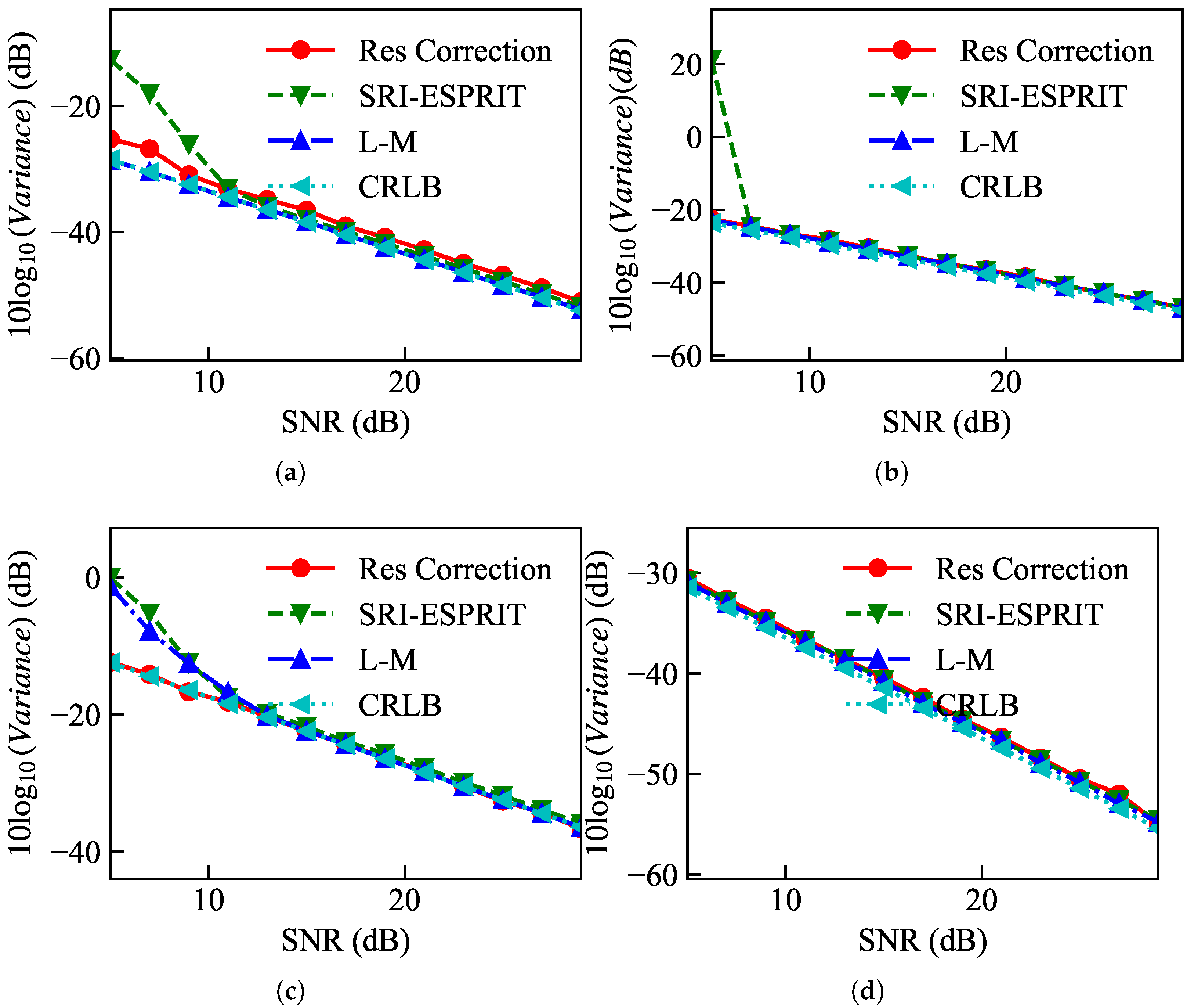
Figure 6 illustrates the performance of different parameter estimation methods under various signal-to-noise ratios. It can be observed that the parameter estimation accuracy of SRI-ESPRIT, Residual Correction, and the L-M algorithm is close to the CRLB. Overall, the SRI-ESPRIT method exhibits the highest parameter estimation accuracy. However, during the process of scatter center matching and association, the estimation of amplitude and bias for different forms of micro-Doppler curves is required. The L-M algorithm and Residual Correction algorithm fail for cosine signals. Therefore, the method adopted in this paper demonstrates superiority in terms of accuracy and stability in parameter estimation.

For the bottom scatter center, after estimating f and $\varphi$ using SRI-ESPRIT, the micro-Doppler decomposition coefficients are obtained through the least squares method. The variances of the decomposition coefficients under different signal-to-noise ratios are shown in Figure 7. It can be observed that as the signal-to-noise ratio increases, the variance of the decomposition coefficients gradually decreases, indicating an improvement in parameter estimation accuracy. The estimated variance of $B_0$ is close to the CRLB, while the estimated variance of $B_1$ is slightly larger than the CRLB, differing by approximately 5 dB. The variances of higher-order decomposition coefficients are even larger, indicating their unsuitability for parameter estimation, which is consistent with theoretical analysis.

5.4. Validation of Multidimensional Parameter Estimation

We construct an optimization model to solve the multidimensional parameters $\{\theta ,{\gamma }_i,{\delta }_i,H,h,r\}$ of the spatial target. Solving the optimization problem yields the parameter estimation results $\{A_A,D_A,B_0,B_1,C_0,C_1\}$. Below, we analyze the parameter estimation results for three scenarios: ${\gamma }_1={50}^{°}$, ${\gamma }_2={120}^{°}$, and ${\gamma }_3={170}^{°}$.

When solving the multi-dimensional parameter estimation model, the parameters are set as $\{H,h,r\}\in (0,5$ m], $\theta \in (0,{15}^{°}]$, ${\delta }_i\in [-5\mathrm{m},5\mathrm{m}]$, and ${\gamma }_i\in [0,{180}^{°}]$ within their respective ranges. The parameters are randomly initialized within these constraints.

Table 5. Parameter estimation results of ${\gamma }_1={50}^{°}$.

Paras	Real	Estimation	RE	RMSE
$\theta$	10°	9.9976	0.0023%	6.1426 × 10−5
${\gamma }_1$	50°	48.4265	3.1509%	0.0154
${\delta }_1$	0.1 m	0.1897	89.7276%	0.0256
H	3 m	2.9750 m	0.8331%	0.0595
h	0.6189 m	0.5352 m	13.5181%	0.0234
r	1 m	1.0858 m	8.5868%	0.0334

presents the parameter estimation results for the case of ${\gamma }_1={50}^{°}$. It can be observed that the RE of ${\delta }_1$ is relatively large at $89.7276\%$. This is because the value set for ${\delta }_1$ itself is too small, and furthermore, the estimated value of ${\delta }_1$ is not involved in target identification. The REs of $\theta$ and H are both less than $1\%$, while those of h and r are $13.5181\%$ and $8.5868\%$ respectively. The RMSE of all parameters is below 0.06, indicating relatively accurate parameter estimation results.

When ${\gamma }_2={120}^{°}$, all three scatter centers A, B, and C are observable.

Table 6. The parameter estimation results using the scatter centers A and B when ${\gamma }_2={120}^{°}$.

Paras	Real	Estimation	RE	RMSE
$\theta$	10°	9.2007°	7.975%	0.0176
${\gamma }_2$	120°	124.6504°	3.8751%	0.3534
${\delta }_2$	0.1 m	0.1560 m	56.0486%	0.1797
H	3 m	2.9983 m	0.0542%	0.4075
h	0.6189 m	0.6558 m	5.9717%	0.2021
r	1 m	1.0829 m	8.2937%	0.3954

presents the parameter estimation results using only scatter centers A and B. Compared to the results obtained when ${\gamma }_1={50}^{°}$, the REs of $\theta$ and ${\gamma }_2$ have increased slightly. However, the RE of parameters ${\delta }_2$, H, h, and r are relatively small, indicating that the radar line of sight angle affects the estimation accuracy of different parameters. The RMSE values are all below 0.4, indicating accurate parameter estimation results.

The different combinations of the three micro-Doppler curves, $r_A$, $r_B$, and $r_C$, provide more possibilities for the estimation of multi-dimensional parameters of the spatial target, assuming that the combinations of solved micro-Doppler curves include $\{A,B\}$, $\{A,B,C\}$, $\{B,C\}$, $\{A,B,BC\}$, and $\{A,B,C,BC\}$, where A, B, C, and $BC$ denote the labels of $r_A$, $r_B$, $r_C$, and $r_B+r_C$, respectively. $\{A,B\}$

Table 7. Relative errors under different combinations of micro-range curves when ${\gamma }_2={120}^{°}$.

Paras	{ $\mathit{A},\mathit{B},\mathit{C}$}	{ $\mathit{B},\mathit{C}$}	{ $\mathit{A},\mathit{B},\mathit{BC}$}	{ $\mathit{A},\mathit{B},\mathit{C},\mathit{BC}$}
$\theta$	1.4241%	24.2053%	1.5446%	1.1698%
${\gamma }_2$	0.1696%	5.9107%	0.2197%	0.167%
${\delta }_2$	1.1377%	225.9851%	2.9228%	0.7722%
H	0.8841%	\	0.6777%	0.7179%
h	0.5951%	43.4331%	0.2868%	0.6625%
r	0.0038%	8.6693%	0.1543%	0.1599%

shows the REs under different combination scenarios. The RE of each parameter under $\{A,B\}$ is shown in Table 6. It can be observed that when using $\{A,B\}$, the RE of H is the smallest, at 0.0542%. Adding the micro-Doppler curve $r_C$ or $r_{BC}$ reduces the REs of $\{\theta ,{\gamma }_i,{\delta }_i,h,r\}$. When only using $\{B,C\}$, the RE of each parameter is relatively large, indicating that the information provided by the micro-Doppler parameters is insufficient.

Using $\{A,B,C\}$, the REs of h and r are the smallest, at 0.0591% and 0.0083%, respectively. Adding the micro-Doppler curve $r_{BC}$ increases the REs of r and h, but at this point, the REs of $\{\theta ,{\gamma }_2,{\delta }_2\}$ estimation results are the smallest among all combinations, at 1.1698%, 0.167%, and 0.7722%, respectively.

Overall, increasing the amount of information improves the accuracy of parameter estimation, but different micro-Doppler curves have varying impacts on the estimation accuracy of different parameters due to differences in the information they provide.

Table 8. Parameter estimation results when ${\gamma }_2={170}^{°}$.

Paras	Real	Estimation	RE	RMSE
$\theta$	10°	8.2887°	17.0967%	0.0271
${\gamma }_3$	170°	170.3674°	0.2148%	0.0483
${\delta }_3$	0.1 m	0.1560 m	304.756%	0.4627
h	0.6189 m	0.9234 m	49.2131%	0.4585
r	1 m	1.1693 m	16.9387%	0.2598

presents the parameter estimation results when ${\gamma }_3={170}^{°}$. It can be observed that the estimation accuracy of ${\gamma }_3$ is relatively high, with an RE of 0.2148%. The RE of $\theta$ and r are below 20%, while the estimation accuracy of other parameters is relatively poor. The RMSE values of all parameters are below 0.5. This is mainly because of the poor observation angle and the insufficient information provided by the two scatter centers at the cone bottom due to their similar expressions. In such cases, multiple radar perspectives are required to improve the accuracy of the parameter estimation.

When observing the spatial target with two radars, with viewing angles ${\gamma }_1={50}^{°}$ and ${\gamma }_2={120}^{°}$ where ${\gamma }_2={120}^{°}$ corresponds to the selection of micro-Doppler curves $\{A,B,C,BC\}$,

Table 9. Parameter estimation results from the joint observations of ${\gamma }_1={50}^{°}$ and ${\gamma }_2={120}^{°}$.

Paras	Real	Estimation	RE	RMSE
$\theta$	10°	9.8941°	1.0398%	0.0026
${\gamma }_1$	50°	50.2830°	0.5621%	0.01640
${\gamma }_2$	120°	119.7441°	0.2135%	0.0131
${\delta }_1$	0.1 m	0.0990 m	0.9389%	0.0245
${\delta }_2$	0.1 m	0.1011 m	1.1467%	0.0168
H	3 m	3.0227 m	1.0944%	0.0493
h	0.6189 m	0.6256 m	1.0944%	0.0138
r	1 m	0.9983 m	0.1695%	0.0237

shows the results of multidimensional parameter estimation. Comparing the results between Table 7 and Table 9 for the single-view case, it can be observed that in the case of dual views, all parameters can be estimated simultaneously with the smallest RE, all below 1.15%. The RMSE values are all below 0.05, indicating accurate and stable parameter estimation results. The redundant information provided by multi-view observations effectively improves the accuracy of multidimensional parameter estimation for spatial targets.

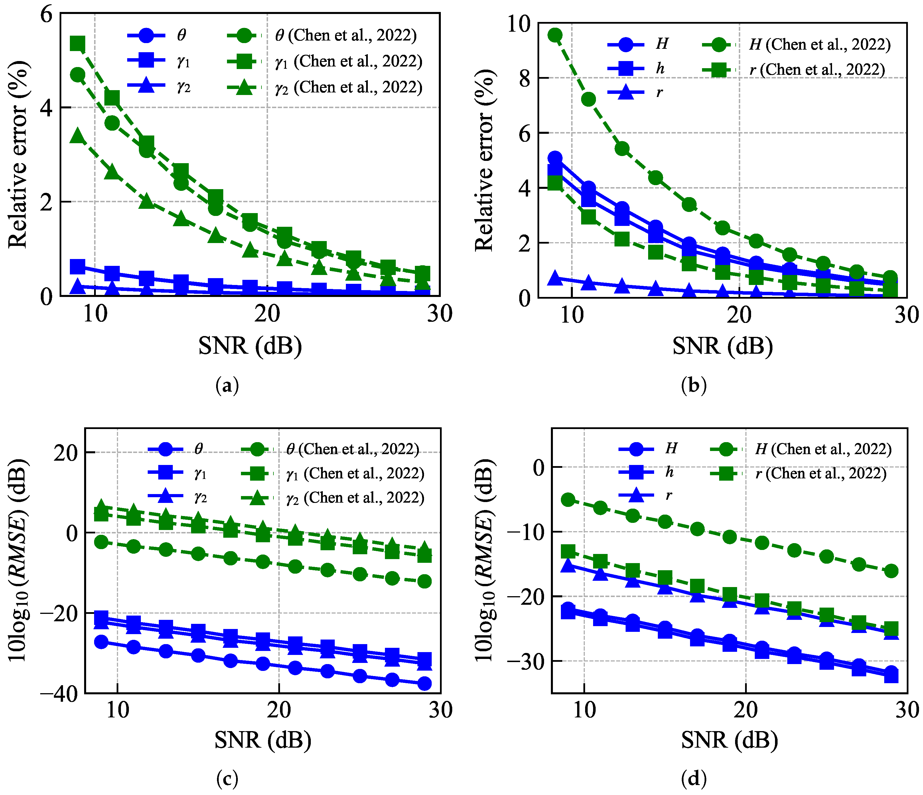
Finally, under double-view observation, we compared the multidimensional parameter estimation method proposed by Chen et al. (2022) [10]. The relative errors (REs) under different signal-to-noise ratios are shown in Figure 8a,b. When the SNR decreases, increased noise in the HRRP signal can distort the shape and continuity of the extracted micro-range curves. Super-resolution frequency estimation algorithms, such as SRI-ESPRIT, are also sensitive to noise, which negatively affects the estimation of micro-range coefficients and reduces the reliability of scattering center association and parameter fitting. These factors severely degrade the accuracy of multidimensional parameter estimation. It can be observed that the RE of the estimated value of $\theta$, ${\gamma }_1$ and ${\gamma }_2$ using the proposed method is smaller than that of Chen et al. (2022) [10]. In addition, the REs of the estimated values of H and h are all smaller when using the proposed method. The performance of the two algorithms varies relative to each other; however, the proposed algorithm exhibits significantly better mean square errors compared to Chen et al. (2022) [10], as shown in Figure 8c,d.

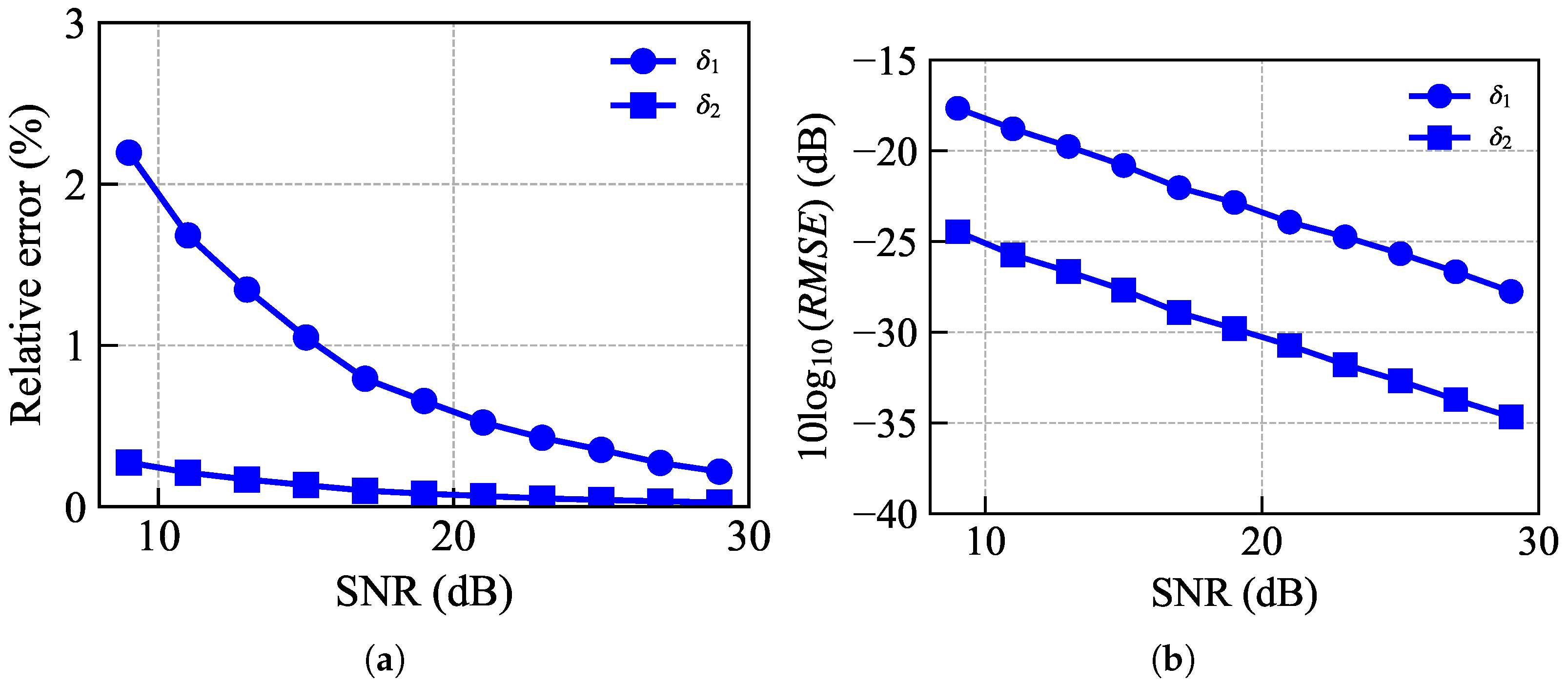
Additionally, the proposed algorithm can effectively estimate the multi-dimensional parameters ${\delta }_1$ and ${\delta }_2$, as shown in Figure 9a,b. It can be observed that the RE and mean square errors of ${\delta }_1$ and ${\delta }_2$ are both below 20% and −15 dB, respectively. The proposed method can mitigate the influence of the target center of gravity and reference distance on parameter estimation performance.

In summary, the proposed method effectively addresses the challenge of multi-dimensional parameter estimation for spatial targets under single and multi-view angles, demonstrating higher accuracy and robustness.

6. Conclusions

Addressing the challenge of multi-dimensional parameter estimation for space cone targets, this paper proposes a method based on micro-range decomposition. By separating the micro-range curves of individual scattering centers from the spatial target echo, the super-resolution algorithm SRI-ESPRIT and the least squares method are employed to estimate the micro-range coefficients, resulting in improved parameter estimation accuracy.

Experimental results demonstrate that when observing the spatial target with two radars at aspect angles ${\gamma }_1={50}^{°}$ and ${\gamma }_2={120}^{°}$, all parameters can be simultaneously estimated, with an RE below 1.15% and RMSE values below 0.05. In the single-view case with ${\gamma }_1={50}^{°}$, most parameters have an RE below 15%, with $\theta$ and H estimated within a 1% error, and all RMSE values remain under 0.06. These results indicate that the proposed method achieves highly accurate parameter estimation in both single-view and dual-view scenarios. Compared with traditional methods, it exhibits lower root-mean-square errors and demonstrates superior robustness and stability.

By effectively leveraging micro-range decomposition and multi-view redundancy, the proposed method significantly improves estimation precision. It can be applied to the high-precision measurement of geometric and micro-motion features for both conical and cone–cylinder mid-course targets.

References

1. Chen, V.C.; Li, F.; Ho, S.-S.; Wechsler, H. Micro-Doppler Effect in Radar: Phenomenon, Model, and Simulation Study. IEEE Trans. Aerosp. Electron. Syst. 2006, 42, 2–21. [Google Scholar]
2. Gao, H.; Xie, L.; Wen, S.; Kuang, Y. Micro-Doppler Signature Extraction from Ballistic Target with Micro-Motions. IEEE Trans. Aerosp. Electron. Syst. 2010, 46, 1969–1982. [Google Scholar] [CrossRef]
3. Xu, Z.; Ai, X.; Wu, Q.; Zhao, F.; Xiao, S. Micro-Doppler Characteristics of Streamlined Ballistic Target. Electron. Lett. 2019, 55, 149–151. [Google Scholar] [CrossRef]
4. Persico, A.R.; Clemente, C.; Gaglione, D.; Ilioudis, C.V.; Cao, J.; Pallotta, L.; De Maio, A.; Proudler, I.; Soraghan, J.J. On Model, Algorithms, and Experiment for Micro-Doppler-Based Recognition of Ballistic Targets. IEEE Trans. Aerosp. Electron. Syst. 2017, 53, 1088–1108. [Google Scholar] [CrossRef]
5. Wei, J.; Peng, J.; Shao, S. High-Precision Micro-motion Parameter Estimation of Sparse Aperture Ballistic Target. In Proceedings of the 2021 International Conference on Control, Automation and Information Sciences (ICCAIS), Jeju, Republic of Korea, 12–15 October 2021; pp. 915–919. [Google Scholar] [CrossRef]
6. Ai, X.; Xu, Z.; Zhao, F. Feature Extraction of Micro-Motional Targets Via Time-Range Distribution. IEEE Access 2019, 7, 118889–118897. [Google Scholar] [CrossRef]
7. Choi, I.O.; Park, S.H.; Kang, K.B.; Lee, S.H.; Kim, K.T. Efficient Parameter Estimation for Cone-Shaped Target Based on Distributed Radar Networks. IEEE Sens. J. 2019, 19, 9736–9747. [Google Scholar] [CrossRef]
8. Hong, L.; Dai, F.; Liu, H. Motion-Parameter Estimation for Precession-with-Nutation Space Targets Based on Wideband Radar Measurements. IEEE Trans. Aerosp. Electron. Syst. 2016, 52, 643–657. [Google Scholar] [CrossRef]
9. Chen, X.; Ye, C.; Dong, C.; Wang, Y.; Hu, Q. Parameter Estimation for Space Precession Targets With Intermittent Observation. IEEE Geosci. Remote Sens. Lett. 2022, 19, 1–5. [Google Scholar] [CrossRef]
10. Chen, X.; Ye, C.; Wang, Y.; Zhang, Y.; Hu, Q. Unambiguous Estimation of Multidimensional Parameters for Space Precession Targets With Wideband Radar Measurements. IEEE Trans. Geosci. Remote Sens. 2022, 60, 5112716. [Google Scholar] [CrossRef]
11. Luo, Y.; Zhang, Q.; Yuan, N.; Zhu, F.; Gu, F. Three-Dimensional Precession Feature Extraction of Space Targets. IEEE Trans. Aerosp. Electron. Syst. 2014, 50, 1313–1329. [Google Scholar] [CrossRef]
12. Taoliu, Y.; Wei, Z.; Xiufen, Z. A Solution of Rotation Invariance Based ESPRIT(SRI-ESPRIT) Method Approach to Direction-of-Arrival Estimation. In Proceedings of the 2012 International Workshop on Microwave and Millimeter Wave Circuits and System Technology, Chengdu, China, 19–20 April 2012; pp. 1–4. [Google Scholar] [CrossRef]
13. Li, L.; Hu, J. Fast-Converging and Low-Complexity Linear Massive MIMO Detection With L-BFGS Method. IEEE Trans. Veh. Technol. 2022, 71, 10656–10665. [Google Scholar] [CrossRef]
14. Yang, D.; Wang, X.; Peng, Z.; Hu, L.; Li, J. Micro-Doppler Separation Based on U-Net and Plot-Curve Association for Ballistic Target. IEEE Trans. Aerosp. Electron. Syst. 2023, 59, 827–836. [Google Scholar] [CrossRef]
15. Shi, Y.; Jiu, B.; Liu, H. Optimization-Based Discontinuous Observation Strategy for Micro-Doppler Signature Extraction of Space Cone Targets. IEEE Access 2019, 7, 58915–58929. [Google Scholar] [CrossRef]
Figure 1. Flowchart of the proposed algorithm.
Remotesensing 17 01294 g001
Figure 2. Spatial cone target precession model.
Remotesensing 17 01294 g002
Figure 3. Spatial cone target model. (a) Geometric Model. (b) Target parameters.
Remotesensing 17 01294 g003
Figure 4. HRRP of a micro-motion target. (a) m-r curves of γ 1 = 50 ° . (b) Association results of γ 1 = 50 ° . (c) m–r curves of γ 2 = 120 ° . (d) Scattering center association results of γ 2 = 120 ° . (e) m–R curves of γ 3 = 150 ° . (f) Association results of γ 3 = 150 ° .
Remotesensing 17 01294 g004
Figure 5. Matching rate of scattering centers.
Remotesensing 17 01294 g005
Figure 6. Comparison of apex parameter estimation results. (a) A 1 . (b) f. (c) ϕ . (d) A 1 .
Remotesensing 17 01294 g006
Figure 7. Estimation results of base parameters. (a) B 0 . (b) B 1 .
Remotesensing 17 01294 g007
Figure 8. Comparison of multidimensional parameter estimation. (a) RE for θ , γ 1 , γ 2 . (b) RE for H , h , r . (c) RMSE for θ , γ 1 , γ 2 . (d) RMSE for H , h , r [10].
Remotesensing 17 01294 g008
Figure 9. Comparison of multidimensional parameter estimation. (a) RE for δ 1 and δ 2 . (b) RMSE for δ 1 and δ 2 .
Remotesensing 17 01294 g009