Assessing the Impact of Mixed Pixel Proportion Training Data on SVM-Based Remote Sensing Classification: A Simulated Study

Abstract

Support vector machine (SVM) algorithms have been widely utilized in the remote sensing community due to their high performance with small training datasets. While previous research has indicated that incorporating mixed pixels into training can enhance the performance of SVM, the impact of the percentage of mixed pixels on classification accuracy remains unexplored. Furthermore, the combined effects of this percentage with other factors including training size, kernel functions (linear, polynomial, radial basis function, and sigmoid), and regularization, have not been thoroughly examined. To address these gaps, this study utilized simulated remote sensing imagery and its corresponding reference map to systematically analyze the impact of these factors on SVM classification accuracy. The results indicate that when the regularization parameter is greater than 1, including mixed pixels in the training generally reduces accuracy, except when a polynomial kernel is used. In contrast, with a lower regularization parameter (<1), at least 50 mixed pixels per class are required in the training dataset to achieve a robust improvement in accuracy. Within these conditions, accuracy increases substantially with a training size up to 300 and a mixed pixel percentage up to 40%. Beyond these thresholds, adding more mixed pixels or training samples leads to minor gains in accuracy. These findings underscore the importance of optimizing the proportion of mixed pixels and carefully selecting regularization parameters to maximize SVM performance in remote sensing applications.

1. Introduction

Image classification is a fundamental technique for producing land use and land cover (LULC) datasets such as GLC 2000 [1], GlobeLand30 [2], and the national land cover database (NLCD) of the United States [3]. These datasets are indispensable for various applications such as natural resource management, urban planning, and climate change modeling [4,5]. The reliability of outcome from these applications highly depends on the accuracy of the LULC datasets used [6,7]. Numerous factors during the classification process may impact the accuracy of the LULC products, such as classification scheme, data sources, machine learning algorithms, availability of ancillary data, and validation design [8,9]. Among these, the collection of training data is crucial for supervised classifiers, as it provides labeled examples needed for the classifier to learn underlying patterns and establish relationships between features and the labels, both of which enable accurate predictions on unseen data [9,10]. Typically, training data are acquired through statistical sampling, with their labels being interpreted via high-resolution images or field surveys [11,12,13].

Support vector machine (SVM) algorithms have been widely adopted in the remote sensing community due to their ability to effectively handle high-dimensional data [10,14]. SVM is a supervised, non-parametric classifier that does not assume any specific statistical distribution of the data [14]. SVM involves three key concepts: hyperplane, kernel, and regularization [15]. First, training the SVM aims to determine a hyperplane, also known as a decision boundary, that optimally separates the training samples into their predefined classes [10]. This hyperplane is positioned to maximize the margin, which is the distance between the hyperplane and the nearest data points (also known as support vectors) from each class [16]. Second, SVM supports both linear and non-linear kernels [17]. A linear kernel assumes that the data features are linearly separable. In contrast, a non-linear kernel addresses more complex relationships between data features by mapping the original feature space into a higher-dimensional space where a hyperplane can be used to separate the classes [15]. The most common non-linear kernels include polynomial, radial basis function (RBF), and sigmoid kernels [18]. The non-linear kernels introduce their own set of parameters. One such parameter, subsequently denoted as gamma ($\gamma$) in this paper, controls the extent of influence a single training point has on the decision boundary [19]. A low gamma value produces a smoother, more generalized decision boundary, whereas a high gamma value makes the model highly sensitive to individual data points, increasing the risk of overfitting. Another parameter is the degree, specifically in the polynomial kernel [19]. This parameter determines the complexity of the function used to transform the input data into a higher-dimensional space. A higher degree allows the model to capture more complex patterns by creating highly nonlinear decision surfaces [19]. Third, the SVM adopts a regularization parameter, subsequently denoted as C in this paper, which controls the trade-off between maximizing the margin and minimizing the classification error [20]. A high value of C places more emphasis on correctly classifying all training examples, which tends to cause an overfitting problem, while a lower value of C allows the model to have a larger margin even if it has some misclassifications during training [18].

Recent advancements in SVM training have focused on key factors such as training dataset size [21,22], class imbalance [23,24], and training efficiency [25,26]. SVM is widely recognized for its ability to achieve high accuracy even with relatively small training datasets. This advantage stems from its training design, where the hyperplane is constructed using support vectors—a subset of training samples positioned near the hyperplane [10]. Recent studies have demonstrated that SVM outperforms random forests (RF) and artificial neural networks (ANN) in crop mapping applications when training data are limited [21,22]. Leveraging this advantage, SVM has been employed as an auxiliary classifier to reduce training size requirements for convolutional neural networks (CNN), particularly in applications involving polarimetric synthetic aperture radar imagery [27]. An imbalanced training set arises when the number of training samples varies significantly between classes [28]. Common strategies to address this issue include rebalancing the dataset through resampling techniques, adapting machine learning algorithms, or employing hybrid approaches that combine both methods [29,30]. Among classifiers such as gradient boosting (GB), adaptive boosting (AdaBoost), RF, and extreme gradient boosting (XGBoost), SVM has demonstrated robustness in handling imbalanced datasets for fruit tree crop classification using Sentinel-2 data [24]. Furthermore, Su et al. (2023) developed a feature rotation-based SVM ensemble method specifically designed for imbalanced hyperspectral image classification [31]. SVM training is expensive computationally and in terms of memory [25,26]. Recent efforts to accelerate training have primarily focused on developing optimization algorithms to effectively identify the support vectors to reduce the training size [25,26,32,33] or on parallelizing the training process [34].

Another factor influencing SVM training is the presence of mixed pixels. Mixed pixels refer to those containing multiple land use and land cover (LULC) classes, each with distinct spectral profiles. Foody and Mathur (2006) demonstrated through several examples that replacing a portion of pure pixels with mixed ones does not negatively impact SVM performance [35]. The underlying reason is that mixed pixels are more likely to be positioned near the hyperplane, potentially becoming support vectors [35]. Yu and Chi (2008) found that SVM classification accuracy trained on a small number of mixed pixels is nearly the same as that achieved with a large quantity of pure pixels [36]. However, Shao and Lunetta (2012) observed that the inclusion of mixed pixels, defined as heterogeneous pixels in their study, in the SVM algorithm did not result in higher accuracy using time-series data derived from a moderate-resolution imaging spectroradiometer (MODIS) [37]. Despite these findings, several gaps remain. First, the effect of mixed pixel proportion in training data on SVM classification accuracy has not been thoroughly examined. Mixed pixels are unavoidable in remote sensing imagery, especially those from satellite sensors with lower spatial resolution. For SVM users collecting training data, key questions arise: Should mixed pixels be included as extensively as possible to enhance classification accuracy for a given SVM kernel? If not, what is the optimal proportion for a given training size? Second, previous studies have not systematically considered the impact of SVM parameters such as kernel functions and regularizations when evaluating the role of mixed pixels. The interaction between mixed pixel proportion, kernel function, and regularization settings—and their collective effect on SVM classification outcomes—remains unexplored.

Beyond SVM classifiers, researchers have also examined the effect of mixed pixels on other classifiers. For example, Kavzoglu and Reis (2013) have found that an ANN classifier with a large amount of mixed pixels performs better in LULC mapping, while a maximum likelihood classifier (MLC) is ineffective when including mixed pixels in training [38]. Costa et al. (2017) investigated the impact of mixed image objects in improving object-based classification accuracy using ANN and a generalized linear model (GLM) and found that incorporating mixed objects into training can increase classification accuracy by around 25% compared to training with pure objects only [39]. The methodologies and findings from these studies provide valuable insights for this research.

Therefore, the objective of this research was to develop an approach to examine how factors, including the percentage of mixed pixels ($MP$), training size, kernel function, and regularization, impact SVM classification accuracy. The study considered four kernel functions: linear, polynomial, RBF, and sigmoid. To comprehensively investigate these factors, a simulation study was conducted to generate the necessary remote sensing image and reference map. This simulation approach enables systematic sampling of different training sizes with varying percentages of mixed pixels, which is nearly impossible using real-world remote sensing imagery. The structure of this paper is as follows: Section 2 describes the study area and details the methodology of the simulating datasets, sampling training data, and configuration parameters for the SVM model. Section 3 presents the results, while Section 4 and Section 5 provide the analysis and conclusions, respectively. This study limits the scope of SVM to hard classification, where each pixel in the classified map has a unique label, although SVM can be applied for spectral unmixing to estimate the proportion of each membership within a mixed pixel [40].

2. Materials and Methods

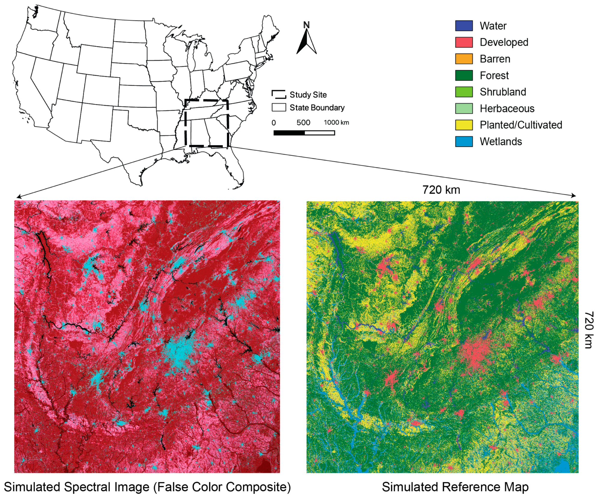
2.1. Study Site

In this study, data simulation was based on the NLCD 2019 data. By utilizing an NLCD dataset, the simulated dataset closely mirrors real-world spatial structures, thereby enhancing the relevance and applicability of the findings. The choice of the study site is therefore crucial, as its spatial characteristics determine the prevalence of mixed pixels relative to pure pixels. A study site in the southeastern United States was selected, covering an area of 720 by 720 km (Figure 1). According to the NLCD 2019 dataset, this region is characterized by a diverse range of land cover types: forest (50.8%), developed land (9.3%), shrubland (3.6%), planted/cultivated areas (22.2%), water bodies (1.9%), herbaceous cover (2.9%), wetlands (9.1%), and barren land (0.2%). Preliminary analysis using Fragstats software v4.3 [41] estimated a mean patch size of 7.0 hectares. The diversity of land cover types, coupled with a relatively fragmented landscape, ensures the presence mixed pixels and the complexity of mixed compositions in the simulated dataset, as described in the following section.

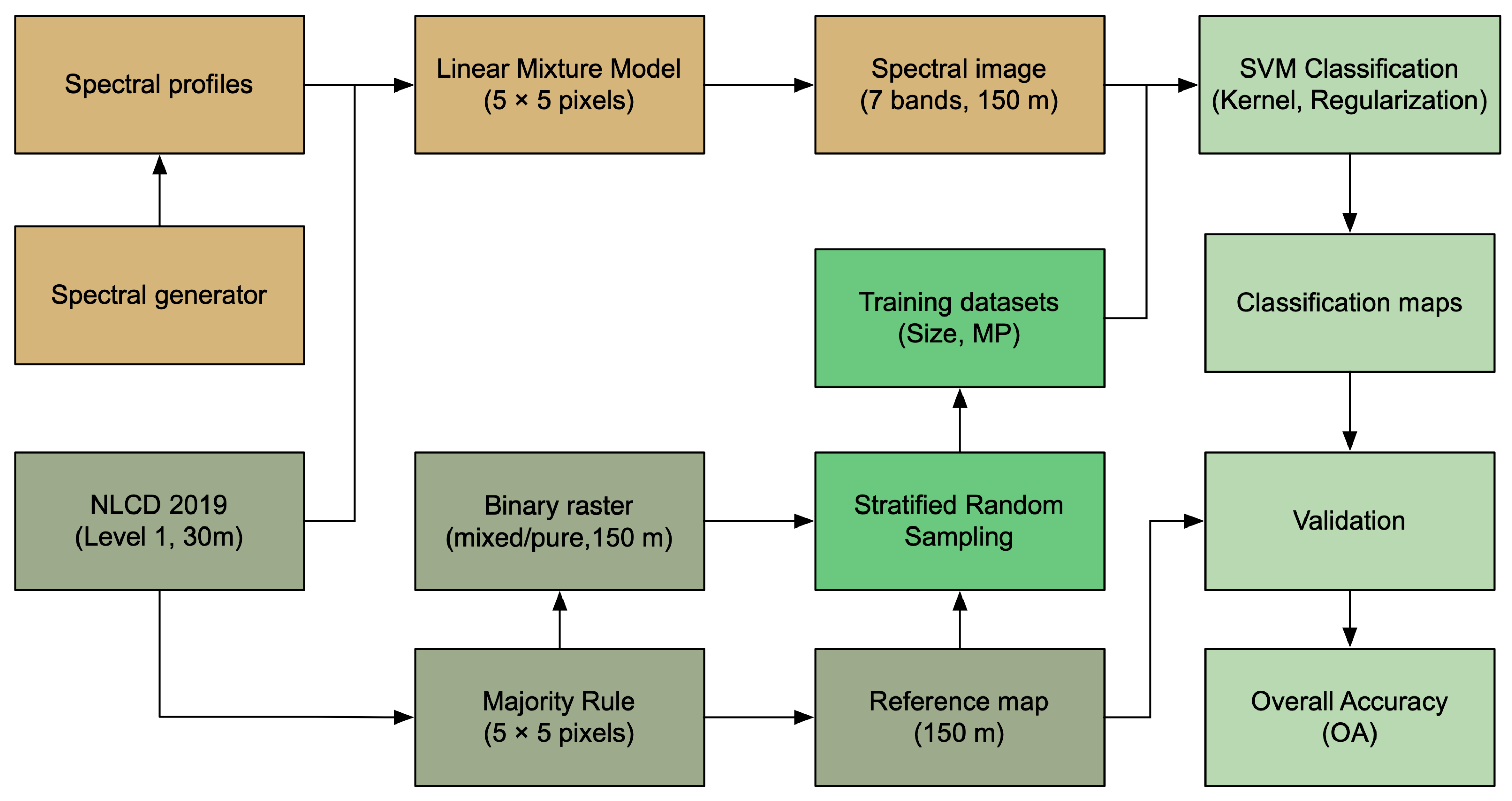
2.2. Outline of Methods

The workflow of this study comprises five key steps (Figure 2). First, a reference map with a spatial resolution of 150 m was generated from the NLCD 2019 dataset (30 m) through aggregation using a majority rule. In this process, each pixel (150 m) in the reference map was assigned a label. Simultaneously, a binary raster was produced to indicate whether each pixel in the reference map was mixed or pure. Second, a spectral image with seven bands was simulated at the same spatial resolution as the reference map. Third, multiple training datasets were randomly sampled from the simulated reference map, with variations in training size and the percentage of mixed pixels. Fourth, SVM classifiers were trained on each of these training datasets using various parameters, including different kernel types and regularization ($C$) values. These trained SVM classifiers were then applied to the simulated image to generate classification maps. Finally, each classification map was compared with the reference map for accuracy assessment.

2.3. Simulate Reference Data

In this study, a reference map with a spatial resolution of 150 m was simulated by aggregating the pixels from the NLCD 2019 dataset at a 30 m spatial scale. The simulation involved two key steps. First, the classification scheme of NLCD 2019, which originally contains 20 classes (level 2 in

Table 1. Two levels of classification scheme. (Level 2 is NLCD 2019 legend, while Level 1 is consolidated from Level 2. The class names with (#) behind them are not contained within the study site).

Level 1	Class Name	Level 2	Class Name
1	Water	11	Open Water
		12	Perennial Ice/Snow (#)
2	Developed	21	Developed, Open space
		22	Developed, Low intensity
		23	Developed, Medium intensity
		24	Developed, High intensity
3	Barren	31	Barren Land
4	Forest	41	Deciduous Forest
		42	Evergreen Forest
		43	Mixed Forest
5	Shrubland	51	Dwarf Scrub (#)
		52	Shrub/Scrub
7	Herbaceous	71	Grassland/Herbaceous
		72	Sedge/Herbaceous (#)
		73	Lichens (#)
		74	Moss (#)
8	Planted/ Cultivated	81	Pasture/Hay
		82	Cultivated Crops
9	Wetlands	90	Woody Wetlands
		95	Emergent Herbaceous Wetlands

), was consolidated into 8 broader classes (level 1 in Table 1) for analysis. This consolidated dataset is referred to as “NLCD-level 1–30 m”. Second, for each $5\times 5$ pixel block in the NLCD-level 1–30 m, a majority rule was applied to determine the dominant label based on frequency. This dominant label was then assigned to the corresponding coarser pixel in the resulting reference map (150 m). If multiple dominant types were identified within a block, then the pixel in the reference map was labeled as “unclassified”. These unclassified locations were excluded from subsequent analysis. The final reference map consists of 4800 × 4800 pixels, with less than 4% categorized as “unclassified”. This reference dataset is designated as “NLCD-Reference-150 m”.

Additionally, during the aggregation process, a binary raster was created to indicate whether each pixel (150 m) in the reference map was pure or mixed based on the homogeneity of each block in the NLCD-level 1–30 m. A block was considered as homogeneous (pure) only if all $5\times 5$ pixels shared the same label. This binary raster, referred to as “NLCD-Mixed-150 m”, was subsequently used to control the percentage of mixed pixels in the training samples drawn from the reference map.

2.4. Simulate a Multispectral Image

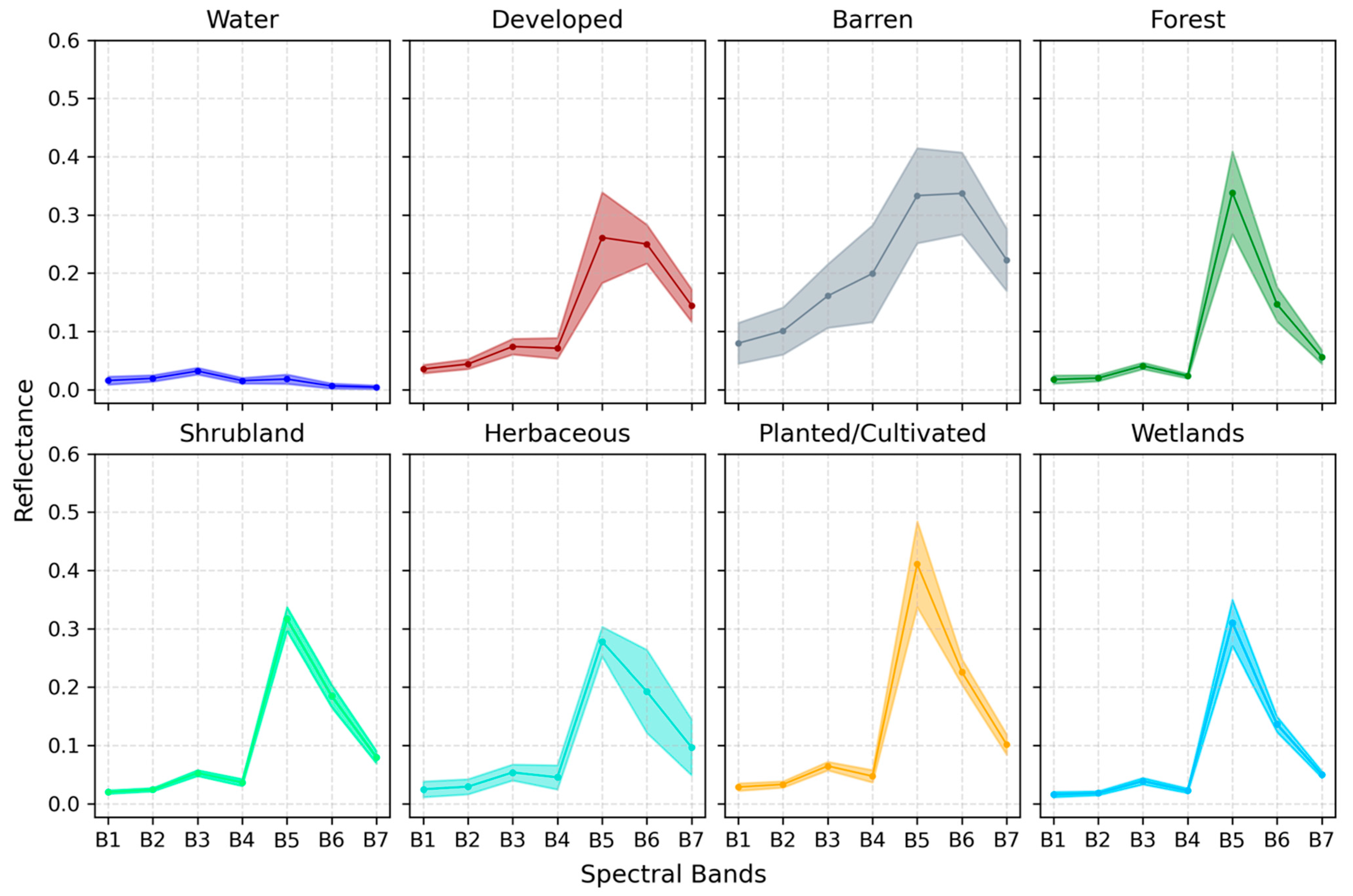
2.4.1. Collect Spectral Profiles for a Label

The goal of this step was to collect pure spectral profiles from imagery that represent a label in NLCD-level 1–30 m (Table 1) within the study site. These profiles were then used to simulate a spectral image. The representativeness of these profiles is ensured by considering the following factors. First, the spectral profiles for a given label should exhibit a consistent pattern in spectral space. For instance, the near-infrared reflectance of a vegetation type is typically higher than its reflectance in the red band. Second, the profiles collected for the same label from different locations should have variation in the feature space, which may be caused by factors such as biophysical processes and the local environment. The collection of these spectral profiles involves the following steps:

First, for each classification label on the NLCD-level 1–30 m within the study site, 400 locations were sampled with each sampling point being centered within a homogeneous patch of the same label, with a minimum size of $7\times 7$ pixels. This approach was employed to ensure that the extracted spectral profiles were as pure as possible, minimizing contamination from adjacent land cover types.

Second, the spectral profile at each sampling location was derived from multiple Landsat 8 images captured between 1 July and 31 August 2019, corresponding to the growing season at the study site. Each spectral profile includes seven bands from the Landsat 8 imagery: coastal aerosol, blue, green, red, near infrared, and two shortwave infrared (SWIR) bands. By collecting spectral profiles throughout the growing season rather than from a single date, this approach ensures that each sampling location has at least one valid spectral profile, thereby minimizing the impact of cloud cover while preserving spectral consistency. For locations where multiple spectral profiles are available due to multiple images being taken during the season, the profiles were averaged across the bands. As a result, each label has 400 spectral profiles. The spectral profiles were obtained from the surface reflectance dataset (USGS Landsat 8 Level 2, Collection 2) available on Google Earth Engine while the preprocessing including cloud and regional masking.

Third, although each sampling location was positioned at the center of a homogeneous patch, the spectral profiles were still subject to noise from factors such as misclassification in the NLCD 2019 dataset. To address this, we excluded spectral profiles with their band values falling outside the range of mean ± 3 standard deviations for that band. This filtering process was applied to 400 spectral profiles per label, effectively removing outliers.

Finally, after the statistical filtering process, the mean and standard deviation for each band of each label were calculated, as shown in Figure 3. These statistical values were then used to fit a normal distribution model, which served as a basis for generating random reflectance values for each band associated with a label during the spectral image simulation described in the following section. The normal model here is referred to as the “spectral-generator”.

2.4.2. Simulate a Spectral Image

A linear mixture model (LMM) [42,43] was applied to simulate a spectral image at the spatial resolution of 150 m (referred to as spectral-image-150 m). The reflectance of a band for a pixel in spectral-image-150 m is derived from a linear combination of this band’s values from the pixel’s endmembers weighted by their respective abundances. Endmembers represent the pure spectral signatures of the constituent land cover types, while abundance refers to the area fraction of each endmember present within a pixel. Consider a pixel in spectral-image-150 m that has $m$ endmembers within the pixel and an image that has $b$ bands. An endmember $j$ has an area fraction $f_j$. Thus, the reflectance $r_i$ of this pixel in the $ith$ band is estimated using the following formula:

$$r_i=\sum _{j=1}^m (a_{ij}{f}_j)$$

(1)

In the formula, $a_{ij}$ denotes the reflectance of the $jth$ endmember in the $ith$ band with $i=1, \dots , b$ and $j=1, \dots , m$. Therefore, the spectral profile, which is a reflectance vector $\mathit{r}$, of a pixel was calculated using the following matrix:

$$\mathit{r}=\mathit{A}\mathit{f}=\left[\begin{array}{ccccc}{a}_{11}& \cdots & a_{1j}& \cdots & a_{1m}\\ ⋮& \ddots & ⋮& \ddots & ⋮\\ a_{i1}& \cdots & a_{ij}& \cdots & a_{im}\\ ⋮& \ddots & ⋮& \ddots & ⋮\\ a_{b1}& \cdots & a_{bj}& \cdots & a_{bm}\end{array}\right]\left[\begin{array}{c}{f}_1\\ ⋮\\ f_j\\ ⋮\\ f_m\end{array}\right]$$

(2)

In the matrix notation, a column $j$ of $\mathit{A}$ represents the $jth$ endmember’s reflectance in all bands, while a row $i$ indicates the $ith$ band’s reflectance values for all endmembers.

In this study, for a coarser pixel in the simulated spectral-image-150 m, the endmembers are the $5\times 5$ pure pixels in NLCD-level 1–30 m that fall within the coarser pixel’s extent. The spectral profile of the coarser pixel was derived using the LMM described above, where the spectral band values of each endmember were sampled from the spectral-generator developed in Section 2.4.1. The abundance of each endmember was estimated based on its area fraction within $5\times 5$ pixels. It is worth noting that the spectral-generator was applied to generate endmember profiles for every coarser pixel in spectral-image-150 m, allowing for variations in the spectral profiles of endmembers during the simulation process.

These simulated datasets have been created to closely resemble real satellite image datasets, though the simulation process has incorporated several simplified models. The primary source of uncertainty arises from the LMM process used to generate spectral pixels. However, the relationships between labels and spectral profiles largely remain intact, as the spectral profiles were directly derived from real images, despite the use of spatial sampling. Again, this simulation approach enables systematic sampling of various training sizes with controlled percentages of mixed pixels for SVM training, which is nearly impossible to achieve with real-world remote sensing imagery.

2.5. SVM Classification

2.5.1. Training Data Selection

This study aimed to explore the impact of training size and the percentage of mixed training samples on SVM classification accuracy. To achieve this, various training datasets were generated. First, a sampling size, denoted as $T_n$, was allocated to each class in NLCD-Reference-150 m. In this study, the sampling size for each class, instead of total size, was used as a control variable for analysis. This approach ensures that the findings of this study remain comparable with others, even if the number of classes varies. Second, within each class in the NLCD-Reference-150 m dataset, a stratified random sampling strategy was applied to select locations. A percentage $\left(MP\right)$ was given to locations identified as mixed pixels based on the NLCD-Mixed-150 m dataset, with the remaining percentage (100-$MP$) assigned to pure pixels. As a result, each sample in a training dataset was characterized by the following attributes: label, mixed or not, and spectral profile extracted from spectral-image-150 m.

In this study, $T_n$ varied across the following values: 80, 100, 200, 300, 400, 500, 600, 800, 1000, and 1200; meanwhile, the $MP$ ranged from 0 to 100% in increments of 10% for each sampling size. However, a single sampling for each pair ($T_n, MP$) may introduce uncertainty in classification performance due to the randomness inherent in sampling locations. To mitigate this, 20 iterations ($I$) of sampling were conducted for each pair. This resulted in a total of 2200 (${10 T}_n\times 11 MP\times 20 I$) training datasets.

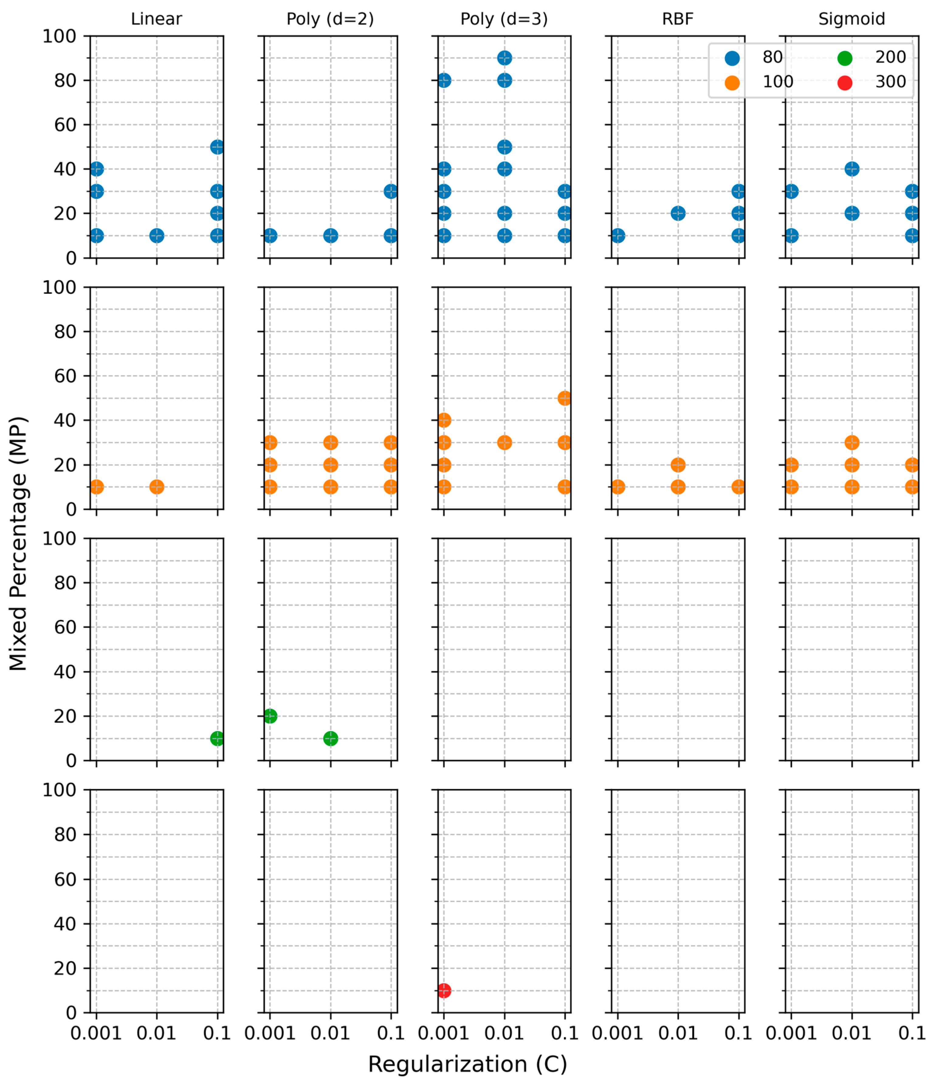
2.5.2. SVM with Various Kernel Parameters

In addition, various kernel functions and regularization parameters ($C$) were explored to evaluate their effectiveness in incorporating mixed pixels in the training data used for classification. The kernel functions ($KF$) tested included linear, polynomial, RBF, and sigmoid. For the polynomial kernel, degrees ($D$) of 2 and 3 were specifically examined. Additionally, to comprehensively assess the impact of regularization ($C)$, a range of $C$ values were tested: 0.001, 0.01, 0.1, 1, 10, and 100. These values were chosen on a logarithmic scale because SVM performance tends to change more rapidly when $C$ is very small or very large, which is a common practice to capture the impact [44]. As a result, 30 parameter combinations were used for training the SVM classifier: 18 combinations for the linear, RBF, and sigmoid kernel functions and 12 combinations for the polynomial kernel function, as the degree D was set to 2 and 3. The parameter configurations for each kernel were detailed in

Table 2. Kernel functions and their corresponding tested parameters. In a kernel equation, $x_i$ and $x_j$ represent the feature vectors of two data points, respectively. The gamma $\left(\mathsf{\gamma }\right)$ is a scaling factor that controls the influence of a single training point. The parameter $d$ represents the degree of the polynomial kernel. A bias or offset term $\mathrm{r}$ shifts the result of the dot product, providing additional flexibility to the model. The symbol “-” indicates that a particular parameter is not applicable to the given kernel.

N.	Kernel	Kernel Equation	Degree	Regularization$\left(\mathit{C}\right)$	Gamma$\left(\mathsf{\gamma }\right)$	Bias$\left(\mathbf{r}\right)$
1	Linear	$\mathrm{K} ({\mathrm{x}}_{\mathrm{i}}, {\mathrm{x}}_{\mathrm{j}})={\mathrm{x}}_{\mathrm{i}}^{\mathrm{T}}{\mathrm{x}}_{\mathrm{j}}$	-	[0.001, 0.01, 0.1, 1, 10, 100]	-	-
2	Polynomial	$\mathsf{{\rm K}} ({\mathrm{x}}_{\mathrm{i}}, {\mathrm{x}}_{\mathrm{j}})={{ (\mathsf{\gamma }·\mathrm{x}}_{\mathrm{i}}^{\mathrm{T}}{\mathrm{x}}_{\mathrm{j}}+\mathrm{r})}^d$	[2,3]		0.1429	0
3	RBF	$\mathsf{{\rm K}} ({\mathrm{x}}_{\mathrm{i}}, {\mathrm{x}}_{\mathrm{j}})=\exp \left({-\mathsf{\gamma }‖x_i-x_j‖}^2\right)$	-			-
4	Sigmoid	$\mathsf{{\rm K}} ({\mathrm{x}}_{\mathrm{i}}, {\mathrm{x}}_{\mathrm{j}})=\tanh { (\mathsf{\gamma }·\mathrm{x}}_{\mathrm{i}}^{\mathrm{T}}{\mathrm{x}}_{\mathrm{j}}+\mathrm{r})$	-			0

. Notably, the gamma parameter was not tested in this study and was instead set to a constant value of 0.1429, equivalent to 1 divided by the number of features (7 spectral bands in this study). For both the polynomial and sigmoid kernels, the bias parameter (r) was set to 0.

Each training dataset generated in Section 2.5.1 was utilized to train a SVM classifier with each parameter combination. The trained classifiers were then applied to spectral-image-150 m to produce classification maps, yielding a total of 66,000 classification maps (30 parameter combinations × 2200 training datasets). The SVM models were trained using scikit-learn (version 1.3.2), an open-source machine learning library [45]. The parameter gamma was set to “auto” in scikit-learn, which automatically calculates its value as 1 divided by the number of features (0.1429 in Table 2).

2.5.3. Accuracy Assessment

Each classification map produced in Section 2.5.2 was evaluated against the NLCD-Reference-150 m dataset derived in Section 2.3 to conduct an accuracy assessment. Typically, an accuracy assessment involves sampling a small subset of the map, which can introduce additional uncertainty into the resulting accuracy metrics [11]. To mitigate this potential source of error, every pixel in the reference dataset—excluding those labeled as “unclassified” and those used for training—was compared with the corresponding pixel in each classification map, i.e., a total enumeration rather than a sample. The approach generated an error matrix, from which the overall accuracy ($OA$) was calculated, ensuring that any variation in classification accuracy could be attributed solely to the training datasets and the SVM classifier parameters.

The $OA$ values were recorded for each combination of $T_n,MP,KF,C,$ and $D$, and then the mean overall accuracy (MOA) and standard deviation of overall accuracy (SDOA) for each group was computed. Each group contains 20 $OA$ values derived from different iterations. Finally, the MOA and SDOA for each group were visualized to examine the impact of these combined factors on classification accuracy.

A right-tailed two-sample t-test was performed to determine whether the MOA of a group containing a certain percentage of mixed pixels (${MOA}_{MP\ne 0}$) was significantly greater than the MOA of a group using pure pixels only (${MOA}_{MP=0}$) while holding all other parameters—$T_n,KF,C,$ and $D$—constant. The null hypothesis is that ${MOA}_{MP\ne 0}$ is not greater than ${MOA}_{MP=0}$, while the alternative hypothesis posits that ${MOA}_{MP\ne 0}$ is greater than ${MOA}_{MP=0}$. The significance level was set at 0.05.

3. Results

Figure 4 illustrates the accuracy of SVM classification using a linear kernel across different $C$ values, while Figure 5, Figure 6, Figure 7 and Figure 8 present the results for other kernels: polynomial (degree = 2), polynomial (degree = 3), RBF, and Sigmoid, respectively. The figure is organized into 12 subfigures: Figure 4a–f show the MOA, while Figure 4g–l display the SDOA. Each sub-figure contains 10 curves representing the different training sizes, with each curve showing how the MOA or SDOA varies as the $MP$ increases from 0 to 100%. This structural layout is consistently used for all figures generated from the analyses employing the other kernels. The findings in Figure 4 are detailed below:

(1)

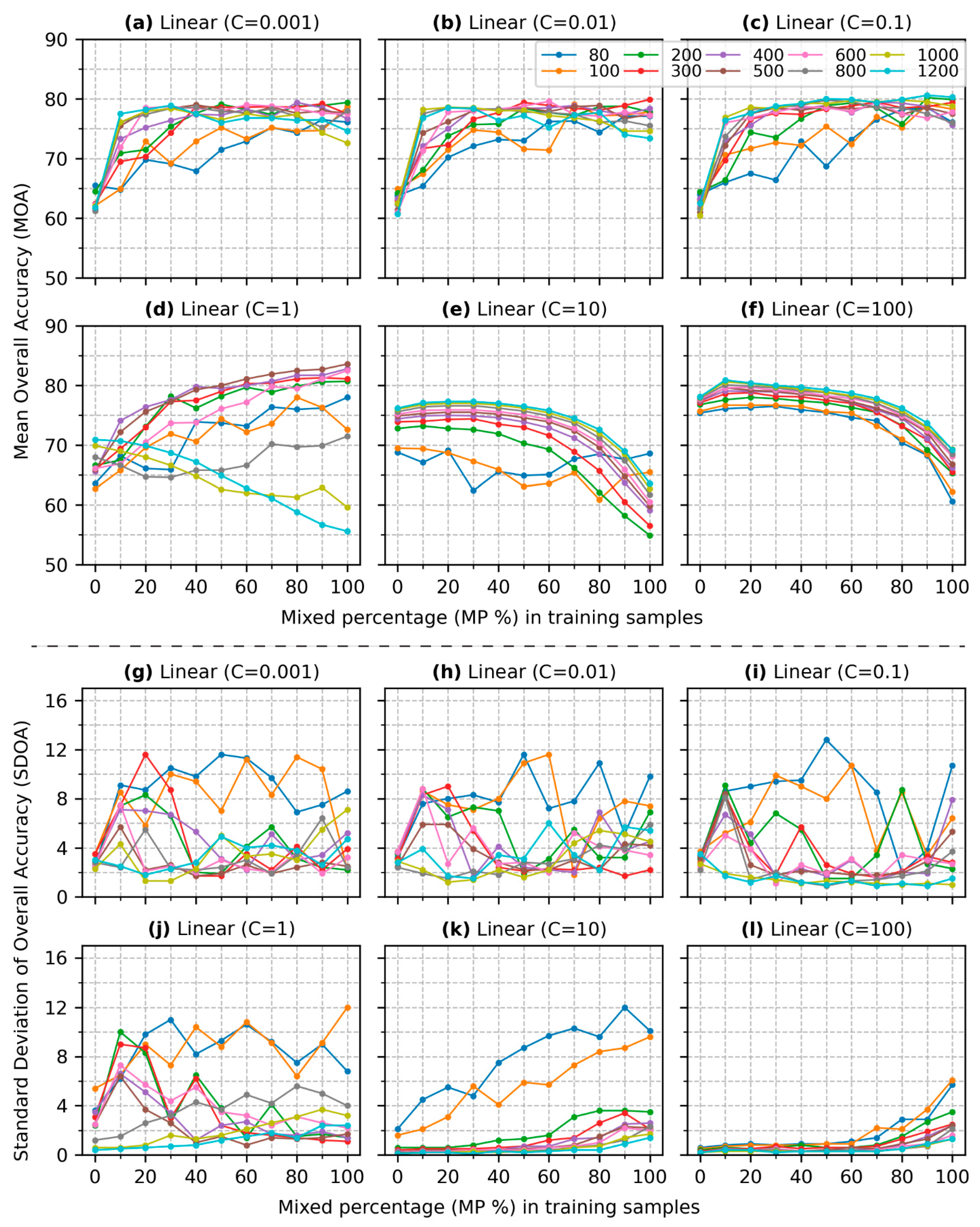
Figure 4a presents the results for a $C$ value of 0.001. When $T_n$ is 80, the MOA begins at 65.5% with no mixed pixels ($MP=0\%$) in the training data. As $MP$ increases from 10% to 100%, the MOA generally exhibits an upward trend, with slight declines observed at $MP$ levels of 10% and 40%. The MOA peaks at 76.1% when the training data consist entirely of mixed pixels ($MP=100\%$). The SDOA (Figure 4g) shows a marked increase from 2.4 to 11.6 as $MP$ rises from 0 to 50%. However, as MP continues to increase to 100%, the SDOA decreases slightly to 8.6. The patterns observed for $T_n=100$ in both MOA and SDOA are consistent with those for $T_n=80$.

(2)

For $T_n$ ranging from 200 to 1200 (Figure 4a), the MOA curves demonstrate a similar upward trend, with larger $T_n$ values leading to higher MOA outcomes. When $MP$ is below 40%, the growth rate of MOA varies with each additional 10% of mixed pixels incorporated into to the training. Notably, the inclusion of 10% mixed pixels results in the most significant increase in MOA, with a maximum improvement of 15.7% observed when $T_n$ = 1200. When $MP$ is over 40%, the MOA lines tend to stabilize, indicating a plateau in accuracy gains. The highest MOA is achieved at 79.4% when $MP$ is 80% and $T_n$ is 400. The SDOA generally reduces as $T_n$ increases from 200 to 1200 (Figure 4g). For instance, when $MP$ is 20, the SDOA value declines from 11.6 to 1.8 as $T_n$ increases from 200 to 1200. In addition, SDOA curves for $T_n$ ranging from 200 to 800 initially rise and then significantly drop when $MP$ approaches 50%.

(3)

The findings for $C$ values of 0.01 and 0.1 (Figure 4b,c) closely resemble those for $C=0.001$ (Figure 4a). Similarly, the SDOA patterns found in Figure 4h,i align with those observed in Figure 4g.

(4)

However, the outcomes in Figure 4d, where $C$ is 1, differ considerably. When $MP$ is 0%, most MOA values in Figure 4d are above 65%, which is higher than the results in Figure 4a. As $MP$ grows, the MOA rises when $T_n$ is below 800. The MOA reaches up to 83.6% when $T_n=500$ and $MP=100$. As the $T_n$ reaches 1000 or higher, incorporating more mixed pixels in the training data leads to lower MOA values.

(5)

The results in Figure 4e, where $C=10$, contrast sharply with those in the previous subfigures. Compared to Figure 4d, the MOA values of $MP,$ being 0% in Figure 4e, are concentrated around 75% except for $T_n=80$ and 100. As $MP$ increases, the MOA values decrease consistently. The SDOA values remain below 4% except for when the $T_n=80$ and 100, which shows a growing trend as $MP$ inclines.

(6)

The findings in Figure 4f are similar to those in Figure 4e. The difference is that MOA values are all above 75% when $MP$ is 0% and decrease as the $MP$ becomes higher. The SDOA values in Figure 4l are generally lower than those in Figure 4k except for $T_n=80$ and 100, which shows a slight increase when $MP$ exceeds 80%.

Figure 4. Overall accuracy (OA) of SVM classification using a linear kernel across various training sizes and mixed percentages. Subfigures (a–f) illustrate the MOA for different regularization parameters while subfigures (g–l) display the SDOA.

Figure 4. Overall accuracy (OA) of SVM classification using a linear kernel across various training sizes and mixed percentages. Subfigures (a–f) illustrate the MOA for different regularization parameters while subfigures (g–l) display the SDOA.

Figure 5. Overall accuracy (OA) of SVM classification using a polynomial kernel (degree = 2) across various training sizes and mixed percentages. Subfigures (a–f) illustrate the MOA for different regularization parameters while subfigures (g–l) display the SDOA.

Figure 5. Overall accuracy (OA) of SVM classification using a polynomial kernel (degree = 2) across various training sizes and mixed percentages. Subfigures (a–f) illustrate the MOA for different regularization parameters while subfigures (g–l) display the SDOA.

Figure 6. Overall accuracy (OA) of SVM classification using a polynomial kernel (degree = 3) across various training sizes and mixed percentages. Subfigures (a–f) illustrate the MOA for different regularization parameters while subfigures (g–l) display the SDOA.

Figure 6. Overall accuracy (OA) of SVM classification using a polynomial kernel (degree = 3) across various training sizes and mixed percentages. Subfigures (a–f) illustrate the MOA for different regularization parameters while subfigures (g–l) display the SDOA.

Figure 7. Overall accuracy (OA) of SVM classification using an RBF kernel across various training sizes and mixed percentages. Subfigures (a–f) illustrate the MOA for different regularization parameters while subfigures (g–l) display the SDOA.

Figure 7. Overall accuracy (OA) of SVM classification using an RBF kernel across various training sizes and mixed percentages. Subfigures (a–f) illustrate the MOA for different regularization parameters while subfigures (g–l) display the SDOA.

Figure 8. Overall accuracy (OA) of SVM classification using a sigmoid kernel across various training sizes and mixed percentages. Subfigures (a–f) illustrate the MOA for different regularization parameters while subfigures (g–l) display the SDOA.

Figure 8. Overall accuracy (OA) of SVM classification using a sigmoid kernel across various training sizes and mixed percentages. Subfigures (a–f) illustrate the MOA for different regularization parameters while subfigures (g–l) display the SDOA.

Figure 5 and Figure 6 present the results of the SVM classification using a polynomial kernel with a degree of 2 and 3, respectively. Compared to the results using a linear kernel in Figure 4, the key findings from these figures are summarized as follows:

(1)

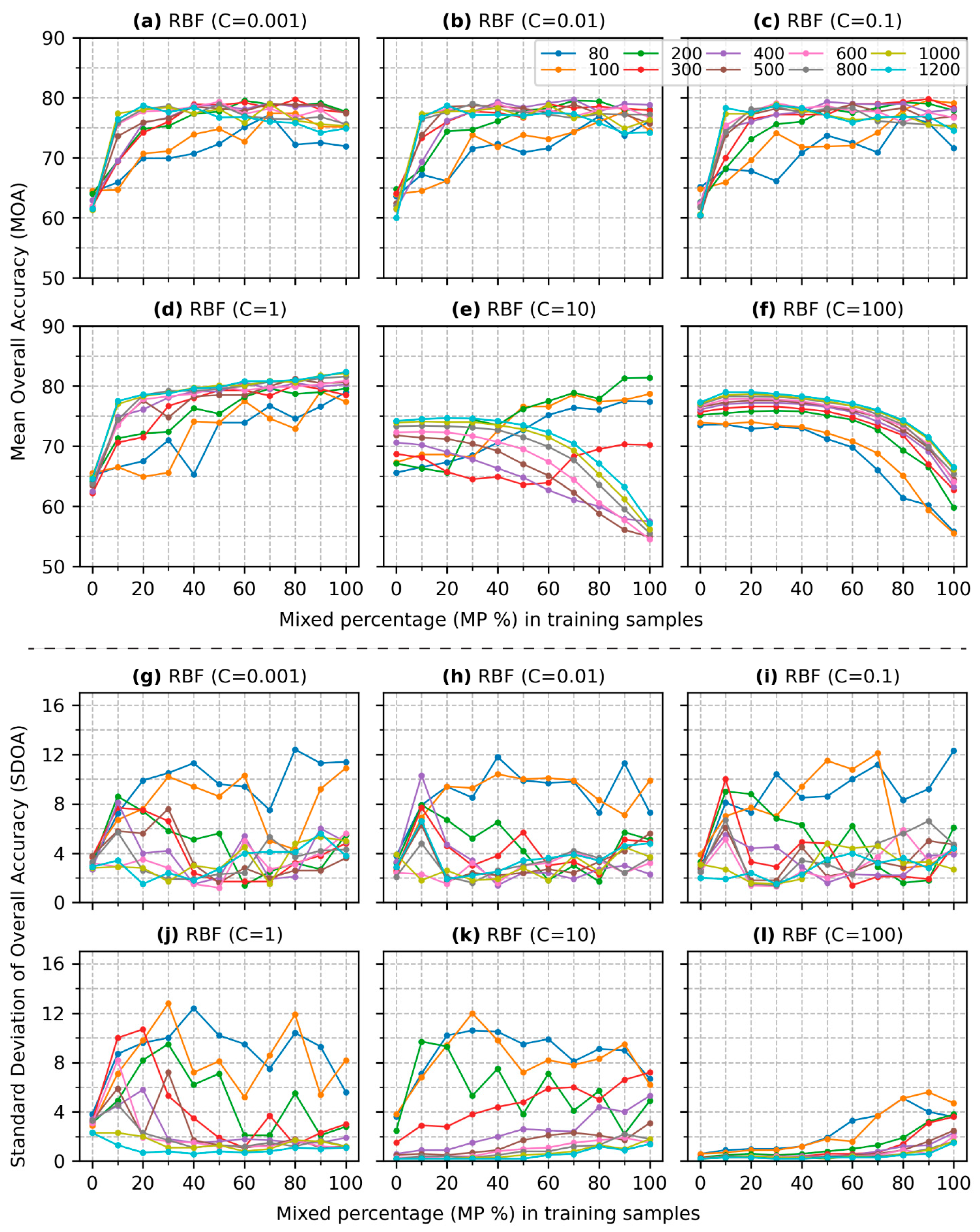
Most MOA values in Figure 5a, derived from pure samples ($MP=0\%$), are under 60%, which is lower the results obtained with a linear kernel in Figure 4a. However, when 10% of mixed pixels are included in the training data, the MOA values increase significantly, except when $T_n=100$. The increase reaches up to 28.3% when $T_n=1000$. As $MP$ increases, the MOA values continue to rise. Similar to Figure 4a, when $MP$ is beyond 40%, the MOA curves tend to stabilize, with the highest accuracy reaching 82.2% when $T_n=1000$ and $MP=100\%$.

(2)

The patterns observed in Figure 5b–e are similar to those in Figure 5a. However, when $C$ becomes 100 (Figure 5f), the MOA decreases with the inclusion of higher $MP$ for $T_n=$ 800, 1000, and 1200. The pattern and trend of SDOA values in Figure 5g–l are similar, with SDOA values generally decreasing as the training size increases.

(3)

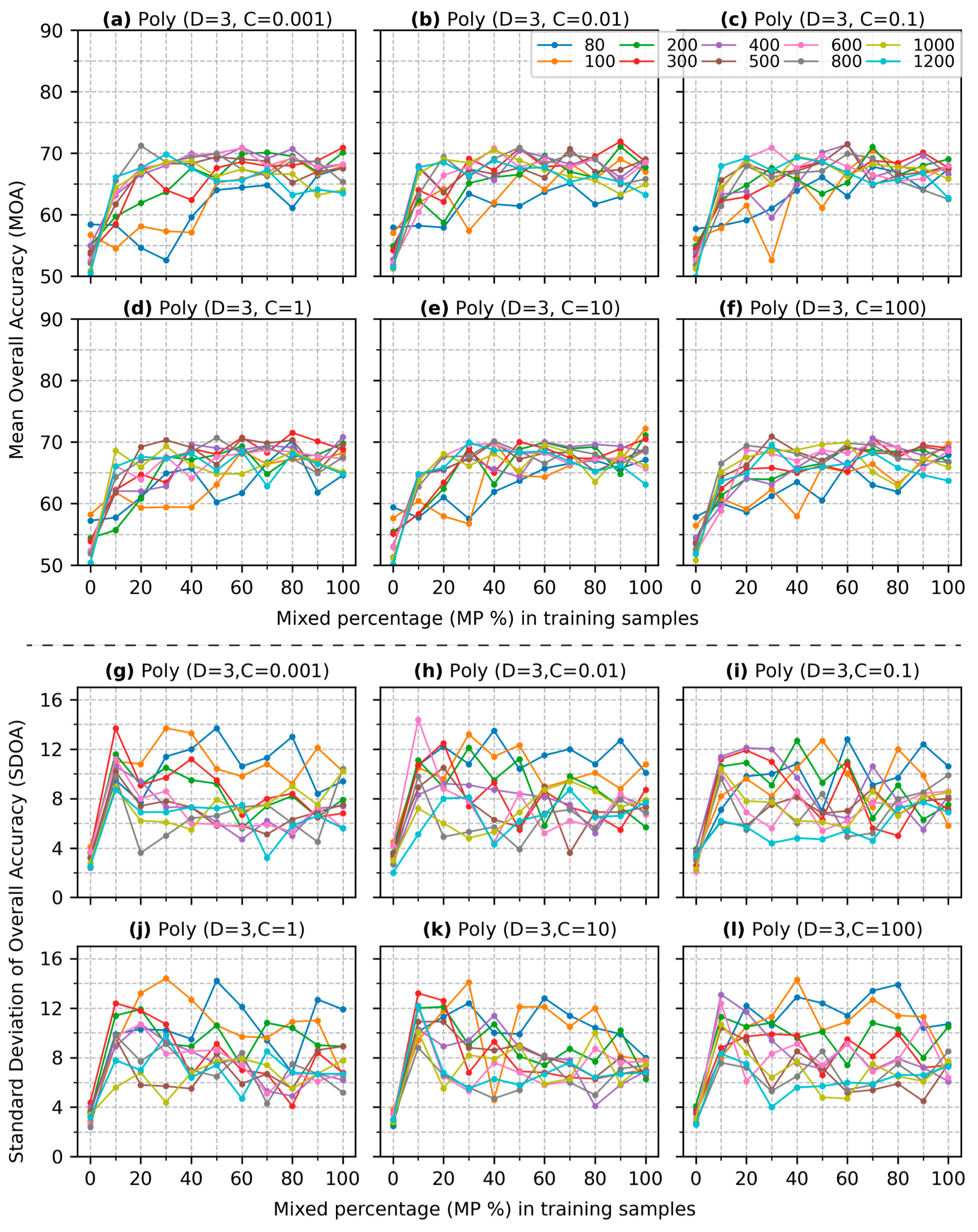
When the degree of the polynomial kernel grows from 2 to 3 (comparing Figure 6 to Figure 5), the patterns of accuracy improvement remain similar, except for that of Figure 6f. All MOA values in Figure 6 are under 60% when $MP$ is 0, and the highest MOA achieves 71.5% when mixed samples are included in the training, compared to a peak MOA of 81.5% in Figure 5. The pattern of a higher $MP$ leading to a higher MOA is consistent across all $C$ values.

(4)

The SDOA values in Figure 6g are higher than those in Figure 5g. The results in Figure 6h,i are close to those in Figure 6g.

Figure 7 provides the results of SVM classification using an RBF kernel. The results in Figure 7 show minor differences compared to those found in Figure 4 except for Figure 7d, which differs more notably from Figure 4d. Unlike Figure 4d, the MOA in Figure 7d goes up with the addition of $MP$.

The findings in Figure 8 are similar to those in Figure 7 except for Figure 8e, where the lines for $T_n=400$ and 500 show an upward trend in contrast to the downward trend observed in Figure 7e.

Figure 9 presents the results of t-tests (represented by dots in each subfigure) for cases where the MOA of a group containing a percentage of mixed pixels (denoted as ${MOA}_{MP\ne 0}$) is not significantly different from the MOA of another group without mixed pixels (${MOA}_{MP=0}$), with all other parameters—$T_n,KF,C$ and $D$—held constant. The figure only shows the non-significant test results and specifically displays results for C $=0.001, 0.01,$ and $0.1$, as higher C values either produce similar outcomes or show a clear downward trend in MOA, as demonstrated in the preceding figures.

In addition, the figure only includes the results for $T_n\le 300$, since all tests yield significant results at larger training sizes. For $T_n=80$, most results across kernels are not statistically significant when $MP$ is 50% or lower. When using a polynomial kernel of degree 3, the groups for ($C=0.001, MP=80\%)$, ($C=0.01, MP=80\%$), and ($C=0.01, MP=90\%$) are also not significant.

When $T_n$ is 100, most non-significant results occur when $MP$ is below 40% except for the case of ($MP=50\%, C=0.1$) with a polynomial kernel of degree 3. When $T_n=200$, all results using the RBF, sigmoid, and polynomial of degree 3 are significant, except for ($C=0.1, MP=10\%)$ with a linear kernel and ($C=0.001, MP=20\%)$ and ($C=0.01, MP=20\%$) with a polynomial kernel of degree 2. When $T_n=300$, the only non-significant result occurs at ($C=0.001, MP=10\%)$ using a polynomial kernel of degree 3.

4. Discussion

While several kernels were tested, the intention was not to determine which kernel performs best, given that the spectral image and reference data were simulated. Instead, our focus was on comparing the efficacy of mixed pixels within a kernel type relative to a baseline where no mixed pixels were included for each training size. The following key questions guided the discussion of our research findings: (1) Does the percentage of mixed pixels in training samples always enhance the accuracy for a given SVM kernel? (2) If not, under what conditions does the mixed percentage begin or cease to affect classification accuracy? (3) Does the mixed percentage influence the training size required for SVM? Specifically, is there an optimal training dataset configuration with a relatively smaller training size but an appropriate mixed percentage that yields higher accuracy? (4) Does regularization have an impact on the findings above?

The results of this study reveal that the inclusion of mixed pixels does not always enhance SVM performance (e) and (f) in Figure 4, Figure 7 and Figure 8. This result is particularly evident when $C$ is greater than 1, where the MOA decreases with a higher $MP$ for all kernels except for the polynomial kernel of degree 3 (Figure 4, Figure 7 and Figure 8). In other words, the SVM performance derived from a training dataset containing mixed pixels cannot compete with the performance of a dataset consisting solely of pure pixels. In SVM classification, a large $C$ value (>1) creates a narrow margin that tends to correctly classify most and sometimes all of the training samples (also known as overfitting) [15,17]. In this case, it increases the importance of mixed pixels used as support vectors. Therefore, a few mixed samples near the hyperplane can determine the hyperplane (i.e., decision boundary). The more mixed samples are included, the greater the likelihood that the hyperplane overfits certain “extreme” mixed samples, which leads to an SVM classifier that loses its ability to generalize to new data. In contrast, when using pure pixels only, a $C$ value greater than 1 can result in a wider margin, as pure pixels are more likely to cluster around the class centroid in the feature space. While the higher $C$ value does not eliminate the risk of overfitting, overfitting on pure pixels still tends to produce a wider margin compared to overfitting on mixed pixels. This result explains why the inclusion of mixed pixels can weaken SVM classification performance when using a $C$ value greater than 1. This study also found that when $C$ is below 1, the MOA increases, with a higher $MP$ for all kernels and training sizes (a), (b), and (c) of Figure 4, Figure 5, Figure 6, Figure 7 and Figure 8 except for the specific cases presented in Figure 9, which will be discussed later. However, as $C$ reaches 1, this trend does not hold for the linear kernel (Figure 4d). Specifically, MOA decreases as $MP$ increases when $T_n$ is above 600 but increases as $MP$ increases when $T_n$ is less than or equal to 600 (Figure 4d). This pattern, where MOA decreases as $MP$ increases at relatively high $T_n$ but increases as $MP$ increases at low $T_n$ is also observed for polynomial kernel (D = 2) when C = 100 and for both RBF and sigmoid kernels when C = 10 (Figure 5f, Figure 7e and Figure 8e). This indicates that when C reaches a certain high value for a specific kernel, a larger training size $T_n$ with a higher $MP$ may lead to reduced performance. A potential explanation is that while a high C value often leads to overfitting on the training data, with smaller training sizes, each data individual point—including mixed pixels—becomes more influential in shaping the model’s decision boundaries. In this case, the mixed samples add valuable complexity and variability to the limited training dataset. However, with larger training sizes, the same $MP$ introduces more mixed pixels, causing SVM to overfit more on the mixed samples that blur class boundaries. As a result, the model’s performance degrades because it becomes less effective at handling the overlapping class information inherent in mixed pixels. These above findings suggest that strategies for incorporating mixed pixels to improve SVM classification performance should involve using a C value lower than 1 to avoid overfitting. Based on this analysis, the subsequent discussion focuses on $C$ values lower than 1.

The findings of this study demonstrate that varying percentages of mixed pixels in the training have different impacts on the improvement of the SVM classification performance. The MOA shows the most improvement when 10% of the training dataset consists of mixed pixels. As the $MP$ increases, the improvement plateaus when $MP$ approaches 40%, with minor gains observed beyond this point (a, b, and c in Figure 4, Figure 5, Figure 6, Figure 7 and Figure 8). However, this study also finds that the SDOA values are relatively higher when $T_n\le 300$ and $MP\le 50\%$ for most kernels except polynomial with a degree of 3 (g, h, and i in Figure 4, Figure 5, Figure 6, Figure 7 and Figure 8). The high standard deviation indicates that the inclusion of mixed pixels is unlikely to improve the SVM accuracy when $T_n\le 100$ and $MP\le 50\%$ and when $200\le T_n\le 300$ and $MP\le 20\%$, which is further supported by the statistical test results in Figure 9. This result signals that a small training size ($\le$100) with a low $MP$ does not enhance SVM performance. A possible interpretation is that the number of mixed samples in these cases is so small that a lower value of $C$ (<1) creates a larger margin, leading to most or even all mixed samples being treated as misclassifications during training. Consequently, there are few or even no mixed samples available for building the hyperplane. Based on these findings, a reliable strategy to improve SVM classification performance is to use a small training dataset (${80\le T}_n\le 100$) with a higher percentage of mixed pixels ($MP\ge 50\%$) except when using a polynomial kernel of degree 3. Another effective strategy is to employ a relatively larger training dataset (${200\le T}_n\le 300$) with $MP>20\%$ or to utilize a training dataset with a size over 300. Furthermore, translating these minimum requirements of training size and $MP$ into the absolute number of mixed samples suggests a rule of thumb: There should be at least 50 mixed pixels for each class in the training dataset to ensure robust performance.

SVM is well regarded for its ability to achieve comparable accuracy even with smaller training datasets [35,39,46]. This capability is evident in our study, as demonstrated by the concentrations of MOA of (a), (b), and (c) in Figure 4, Figure 5, Figure 6, Figure 7 and Figure 8, with lower a SDOA of (g), (h), and (i) in Figure 4, Figure 5, Figure 6, Figure 7 and Figure 8 when the training data consist solely of pure pixels. However, a small training dataset (${80\le T}_n\le 100$) with a low percentage ($MP\le 50\%$) of mixed pixels introduces greater variability in SVM performance, as reflected in the higher SDOA. This variability suggests that while SVM can perform well with smaller training datasets, the inclusion of mixed pixels provides a minimum threshold for both training size and $MP$ (${200\le T}_n\le 300$ and $MP>20\%$ or $T_n>300$) to ensure more consistent and reliable classification outcomes. Importantly, meeting these minimum requirements does not imply that a larger training size or a higher percentage of mixed pixels will always yield better performance. For instance, a training size of $T_n=300$ with $MP=40\%$ can achieve a classification accuracy comparable to that of any larger training size or higher mixed pixel percentage. This finding underscores that beyond a certain point, increasing the training size or mixed pixel percentage does not provide substantial benefits and highlights the need for optimizing these parameters to balance performance and computational efficiency in SVM classification for remote sensing applications.

The existence of mixed pixels in training data is inevitable, particularly when using satellite imagery with coarser spatial resolutions, such as Landsat and MODIS (moderate-resolution imaging spectroradiometer) imagery [47]. Although this study found benefits in including mixed pixels for training SVM, care is required, as under certain conditions for selected regularization parameters, training sizes, and mixed pixel percentages, these mixed pixels will introduce noise into the classification in the form of mislabeled samples due to manual misinterpretation during data collection. Mixed pixels typically occur at the edges of different land cover classes where their spectral profiles may resemble more than one class. For instance, a mixed pixel containing 50% forest, 45% grass, and 5% barren land could have a spectral signature that resembles either forest or grass, leading to potential misinterpretation by the data collector. Previous research has shown that the overall accuracy of SVM could decrease by up to 8% if mislabeled cases constitute 20% of the training data [48]. Although mixed samples with some conditions found above could be used to improve the accuracy, future research should carefully weigh the advantages of incorporating mixed pixels to improve SVM performance against the risk of misinterpretation.

Several uncertainties exist in this study that could be improved in future research. First, this study utilized a linear model to simulate the spectral image and reference map for controlled experiments, which may not fully capture the complexities of real-world satellite imagery. Future studies could consider using more advanced models such as probabilistic or geometric–optical models or testing with actual satellite images [43]. The results in this study provide useful insights regarding the optimal training size, percentage of mixed pixels, and SVM kernels, serving as a foundation for future research directions. Second, the spectral profiles in this study were limited to the seven bands of Landsat 8 imagery. Future research could expand the analysis to datasets with a greater number of spectral bands, such as hyperspectral imagery, or to derived datasets like time-series Normalized Difference Vegetation Index (NDVI), both of which are increasingly used for LULC mapping [49]. Incorporating additional features could enhance classification accuracy and provide a more comprehensive understanding of mixed pixels. Third, this study focused on a single study site with a classification scheme of eight classes, even though the site covered an extensive area of 518,400 km². Different study sites with varied landscape characteristics or alternative classification schemes could significantly alter the mixed pixel composition of the image. Future research should consider multiple study sites with diverse landscape features to validate the robustness of the SVM classification approach across different environments. This would help in understanding how different landscapes and classification schemes affect the presence and impact of mixed pixels on SVM classification accuracy. Finally, this study did not systematically test all parameters associated with specific kernels, such as the gamma parameter for the polynomial kernel. This limitation was partially due to the intensive computation demands, as the classification process in this study took 187 days on a workstation equipped with an Intel-Core i9-12,900 K processor (16 cores), 64 GB of RAM, and a 2 TB solid-state drive. Nonetheless, the findings in this study provide a solid foundation for future research to further explore and expand upon. In summary, while this study provides important insights into the effects of mixed pixels on SVM classification accuracy, there are several areas for improvement and expansion. Addressing these uncertainties in future research will contribute to developing more accurate and reliable remote sensing classification methodologies.

5. Conclusions

Previous studies have shown that incorporating mixed pixels in training can achieve comparable or even higher accuracy in remote sensing classification using SVM. However, they did not investigate the effects of percentage of mixed pixels, training size, regularization, and kernel types. This study addressed these research gaps by systematically examining these factors to understand their impact on SVM classification accuracy. The use of simulated datasets enabled a controlled experiment, allowing for the sampling of large sets of training data with varying sizes and percentages of mixed pixels combined with various kernels and regularization parameters for SVM classification. The conclusions and suggestions of this study are summarized below:

(1)

The incorporation of mixed pixels in training does not always enhance SVM performance. When regularization parameter $(C)$ is greater than 1, the MOA decreases, with a higher $MP$ for all kernels except for the polynomial kernel of degree 3.

(2)

When the regularization parameter is lower than 1, a general of rule of thumb is to include at least 50 mixed pixels per class in the training dataset to ensure a robust improvement in classification.

(3)

Within these conditions, accuracy increases substantially, with a training size up to 300 and a mixed pixel percentage up to 40%. Beyond these thresholds, adding more mixed pixels or training samples leads to minor gains in accuracy. A training dataset with $T_n=300$ and $MP=40\%$ can achieve a classification accuracy comparable to that of any larger training size or higher mixed pixel percentage.

(4)

Optimizing the proportion of mixed pixels and carefully selecting regularization parameters are crucial for maximizing SVM performance in remote sensing applications.

(5)

Despite these findings, this study has several limitations, including the simulation of spectral images and reference data, the selection of spectral profiles, and the choice of study sites. The gamma parameter in the SVM model was held constant, which represents another factor that could be explored in future studies. Additionally, mixed pixels are more challenging to interpret than pure pixels, which may lead to mislabeling in the training process. Future research should carefully balance the benefits of incorporating mixed pixels to enhance SVM performance against the risk of misinterpretation.

References

- Bartholomé, E.; Belward, A.S. GLC2000: A new approach to global land cover mapping from Earth observation data. Int. J. Remote Sens. 2005, 26, 1959–1977. [Google Scholar]
- Chen, J.; Chen, J.; Liao, A.; Cao, X.; Chen, L.; Chen, X.; Mills, J. Global land cover mapping at 30 m resolution: A POK-based operational approach. ISPRS J. Photogramm. Remote Sens. 2015, 103, 7–27. [Google Scholar]
- Jin, S.; Homer, C.; Yang, L.; Danielson, P.; Dewitz, J.; Li, C.; Zhu, Z.; Xian, G.; Howard, D. Overall Methodology Design for the United States National Land Cover Database 2016 Products. Remote Sensing 2019, 11, 2971. [Google Scholar] [CrossRef]
- Mantyka-Pringle, C.S.; Visconti, P.; Di Marco, M.; Martin, T.G.; Rondinini, C.; Rhodes, J.R. Climate change modifies risk of global biodiversity loss due to land-cover change. Biol. Conserv. 2015, 187, 103–111. [Google Scholar]
- Padbhushan, R.; Kumar, U.; Sharma, S.; Rana, D.S.; Kumar, R.; Kohli, A.; Kumari, P.; Parmar, B.; Kaviraj, M.; Sinha, A.K.; et al. Impact of Land-Use Changes on Soil Properties and Carbon Pools in India: A Meta-analysis. Front. Environ. Sci. 2022, 9, 794866. [Google Scholar]
- Feddema, J.J.; Oleson, K.W.; Bonan, G.B.; Mearns, L.O.; Buja, L.E.; Meehl, G.A.; Washington, W.M. The importance of land-cover change in simulating future climates. Science 2005, 310, 1674–1678. [Google Scholar]
- Zhao, L.; Lee, X.; Smith, R.B.; Oleson, K. Strong contributions of local background climate to urban heat islands. Nature 2014, 511, 216–219. [Google Scholar]
- Congalton, R.G.; Gu, J.; Yadav, K.; Thenkabail, P.; Ozdogan, M. Global Land Cover Mapping: A Review and Uncertainty Analysis. Remote Sens. 2014, 6, 12070–12093. [Google Scholar] [CrossRef]
- Maxwell, A.E.; Warner, T.A.; Fang, F. Implementation of machine-learning classification in remote sensing: An applied review. Int. J. Remote Sens. 2018, 39, 2784–2817. [Google Scholar]
- Mountrakis, G.; Im, J.; Ogole, C. Support vector machines in remote sensing: A review. ISPRS J. Photogramm. Remote Sens. 2011, 66, 247–259. [Google Scholar]
- Congalton, R.G.; Green, K. Assessing the Accuracy of Remotely Sensed Data: Principles and Practices; CRC Press: Boca Raton, FL, USA, 2019. [Google Scholar]
- Shetty, S.; Gupta, P.K.; Belgiu, M.; Srivastav, S.K. Assessing the Effect of Training Sampling Design on the Performance of Machine Learning Classifiers for Land Cover Mapping Using Multi-Temporal Remote Sensing Data and Google Earth Engine. Remote Sens. 2021, 13, 1433. [Google Scholar] [CrossRef]
- Jin, H.; Stehman, S.V.; Mountrakis, G. Assessing the impact of training sample selection on accuracy of an urban classification: A case study in Denver, Colorado. Int. J. Remote Sens. 2014, 35, 2067–2081. [Google Scholar] [CrossRef]
- Maulik, U.; Chakraborty, D. Remote Sensing Image Classification: A survey of support-vector-machine-based advanced techniques. IEEE Geosci. Remote Sens. Mag. 2017, 5, 33–52. [Google Scholar] [CrossRef]
- Scholkopf, B.; Smola, A.J. Learning with Kernels: Support Vector Machines, Regularization, Optimization, and Beyond; MIT Press: Cambridge, MA, USA, 2018. [Google Scholar]
- Cervantes, J.; Garcia-Lamont, F.; Rodríguez-Mazahua, L.; Lopez, A. A comprehensive survey on support vector machine classification: Applications, challenges and trends. Neurocomputing 2020, 408, 189–215. [Google Scholar] [CrossRef]
- Patle, A.; Chouhan, D.S. SVM kernel functions for classification. In Proceedings of the 2013 International Conference on Advances in Technology and Engineering (ICATE), Mumbai, India, 23–25 January 2013. [Google Scholar]
- Wang, L. Support Vector Machines: Theory and Applications; Springer: Berlin/Heidelberg, Germany, 2005; Volume 177. [Google Scholar]
- Nalepa, J.; Kawulok, M. Selecting training sets for support vector machines: A review. Artif. Intell. Rev. 2019, 52, 857–900. [Google Scholar] [CrossRef]
- Sheykhmousa, M.; Mahdianpari, M.; Ghanbari, H.; Mohammadimanesh, F.; Ghamisi, P.; Homayouni, S. Support Vector Machine Versus Random Forest for Remote Sensing Image Classification: A Meta-Analysis and Systematic Review. IEEE J. Sel. Top. Appl. Earth Obs. Remote Sens. 2020, 13, 6308–6325. [Google Scholar] [CrossRef]
- Croci, M.; Impollonia, G.; Blandinières, H.; Colauzzi, M.; Amaducci, S. Impact of Training Set Size and Lead Time on Early Tomato Crop Mapping Accuracy. Remote Sensing 2022, 14, 4540. [Google Scholar] [CrossRef]
- Gao, Z.; Guo, D.; Ryu, D.; Western, A.W. Training sample selection for robust multi-year within-season crop classification using machine learning. Comput. Electron. Agric. 2023, 210, 107927. [Google Scholar] [CrossRef]
- Heydari, S.S.; Mountrakis, G. Effect of classifier selection, reference sample size, reference class distribution and scene heterogeneity in per-pixel classification accuracy using 26 Landsat sites. Remote Sens. Environ. 2018, 204, 648–658. [Google Scholar] [CrossRef]
- Chabalala, Y.; Adam, E.; Ali, K.A. Exploring the Effect of Balanced and Imbalanced Multi-Class Distribution Data and Sampling Techniques on Fruit-Tree Crop Classification Using Different Machine Learning Classifiers. Geomatics 2023, 3, 70–92. [Google Scholar] [CrossRef]
- Kurbakov, M.Y.; Sulimova, V.V. Fast SVM-based One-Class Classification in Large Training Sets. In Proceedings of the 2023 IX International Conference on Information Technology and Nanotechnology (ITNT), Samara, Russia, 17–21 April 2023; pp. 1–6. [Google Scholar]
- Zhang, J.; Liu, C. Fast instance selection method for SVM training based on fuzzy distance metric. Appl. Intell. 2023, 53, 18109–18124. [Google Scholar] [CrossRef]
- Zhao, M.; Cheng, Y.; Qin, X.; Yu, W.; Wang, P. Semi-Supervised Classification of PolSAR Images Based on Co-Training of CNN and SVM with Limited Labeled Samples. Sensors 2023, 23, 2109. [Google Scholar] [CrossRef] [PubMed]
- Douzas, G.; Bacao, F.; Fonseca, J.; Khudinyan, M. Imbalanced Learning in Land Cover Classification: Improving Minority Classes’ Prediction Accuracy Using the Geometric SMOTE Algorithm. Remote Sens. 2019, 11, 3040. [Google Scholar] [CrossRef]
- Paoletti, M.E.; Mogollon-Gutierrez, O.; Moreno-Álvarez, S.; Sancho, J.C.; Haut, J.M. A Comprehensive Survey of Imbalance Correction Techniques for Hyperspectral Data Classification. IEEE J. Sel. Top. Appl. Earth Obs. Remote Sens. 2023, 16, 5297–5314. [Google Scholar] [CrossRef]
- Chen, W.; Yang, K.; Yu, Z.; Shi, Y.; Chen, C.L.P. A survey on imbalanced learning: Latest research, applications and future directions. Artif. Intell. Rev. 2024, 57, 1–51. [Google Scholar] [CrossRef]
- Su, Y.; Li, X.; Yao, J.; Dong, C.; Wang, Y. A Spectral–Spatial Feature Rotation-Based Ensemble Method for Imbalanced Hyperspectral Image Classification. IEEE Trans. Geosci. Remote Sens. 2023, 61, 1–18. [Google Scholar] [CrossRef]
- Chowdhury, K.; Chaudhuri, D.; Pal, A.K. A faster SVM classification technique for remote sensing images using reduced training samples. J. Ambient. Intell. Humaniz. Comput. 2023, 14, 16807–16827. [Google Scholar] [CrossRef]
- Xu, B.; Wen, Z.; Yan, L.; Zhao, Z.; Yin, Z.; Liu, W.; He, B. Leveraging Data Density and Sparsity for Efficient SVM Training on GPUs. In Proceedings of the 2023 IEEE International Conference on Data Mining (ICDM), Shanghai, China, 1–4 December 2023; pp. 698–707. [Google Scholar]
- Tavara, S. Parallel Computing of Support Vector Machines: A Survey. ACM Comput. Surv. 2019, 51, 1–38. [Google Scholar] [CrossRef]
- Foody, G.M.; Mathur, A. The use of small training sets containing mixed pixels for accurate hard image classification: Training on mixed spectral responses for classification by a SVM. Remote Sens. Environ. 2006, 103, 179–189. [Google Scholar] [CrossRef]
- Yu, B.-H.; Chi, K.-H. Support vector machine classification using training sets of small mixed pixels: An appropriateness assessment of IKONOS imagery. Korean J. Remote Sens. 2008, 24, 507–515. [Google Scholar]
- Shao, Y.; Lunetta, R.S. Comparison of support vector machine, neural network, and CART algorithms for the land-cover classification using limited training data points. ISPRS J. Photogramm. Remote Sens. 2012, 70, 78–87. [Google Scholar] [CrossRef]
- Kavzoglu, T.; Reis, S. Performance Analysis of Maximum Likelihood and Artificial Neural Network Classifiers for Training Sets with Mixed Pixels. GIScience Remote Sens. 2013, 45, 330–342. [Google Scholar]
- Costa, H.; Foody, G.M.; Boyd, D.S. Using mixed objects in the training of object-based image classifications. Remote Sens. Environ. 2017, 190, 188–197. [Google Scholar] [CrossRef]
- Li, X.; Jia, X.; Wang, L.; Zhao, K. On Spectral Unmixing Resolution Using Extended Support Vector Machines. IEEE Trans. Geosci. Remote Sens. 2015, 53, 4985–4996. [Google Scholar]
- McGarigal, K.; Marks, B.J. FRAGSTATS: Spatial Pattern Analysis Program for Quantifying Landscape Structure; U.S. Department of Agriculture, Forest Service, Pacific Northwest Research Station: Portland, OR, USA, 1995. [Google Scholar]
- Small, C. High spatial resolution spectral mixture analysis of urban reflectance. Remote Sens. Environ. 2003, 88, 170–186. [Google Scholar] [CrossRef]
- Ichoku, C.; Karnieli, A. A review of mixture modeling techniques for sub-pixel land cover estimation. Remote Sens. Rev. 1996, 13, 161–186. [Google Scholar]
- Tharwat, A. Parameter investigation of support vector machine classifier with kernel functions. Knowl. Inf. Syst. 2019, 61, 1269–1302. [Google Scholar]
- Pedregosa, F.; Varoquaux, G.; Gramfort, A.; Michel, V.; Thirion, B.; Grisel, O.; Duchesnay, É. Scikit-learn: Machine learning in Python. J. Mach. Learn. Res. 2011, 12, 2825–2830. [Google Scholar]
- Foody, G.M.; Mathur, A. Toward intelligent training of supervised image classifications: Directing training data acquisition for SVM classification. Remote Sens. Environ. 2004, 93, 107–117. [Google Scholar]
- Justice, C.; Townshend, J.; Vermote, E.; Masuoka, E.; Wolfe, R.; Saleous, N.; Roy, D.; Morisette, J. An overview of MODIS Land data processing and product status. Remote Sens. Environ. 2002, 83, 3–15. [Google Scholar]
- Foody, G.M. The effect of mis-labeled training data on the accuracy of supervised image classification by SVM. In Proceedings of the 2015 IEEE International Geoscience and Remote Sensing Symposium (IGARSS), Milan, Italy, 13–18 July 2015. [Google Scholar]
- He, Y.; Lee, E.; Warner, T.A. A time series of annual land use and land cover maps of China from 1982 to 2013 generated using AVHRR GIMMS NDVI3g data. Remote Sens. Environ. 2017, 199, 201–217. [Google Scholar] [CrossRef]