
Assessing Heterogeneity of Surface Water Temperature Following Stream Restoration and a High-Intensity Fire from Thermal Imagery


Abstract
1. Introduction
2. Methods
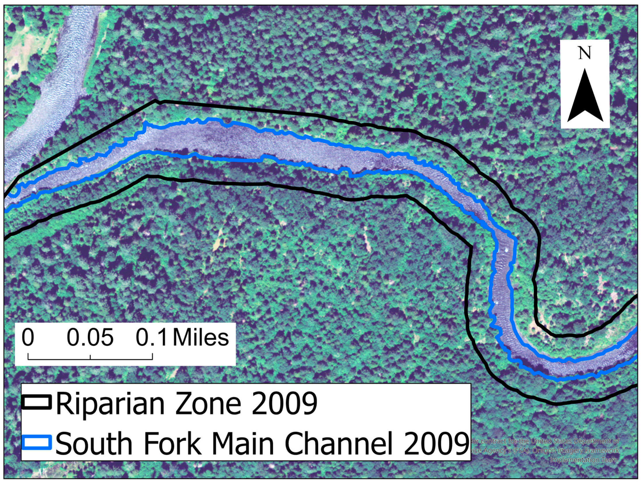
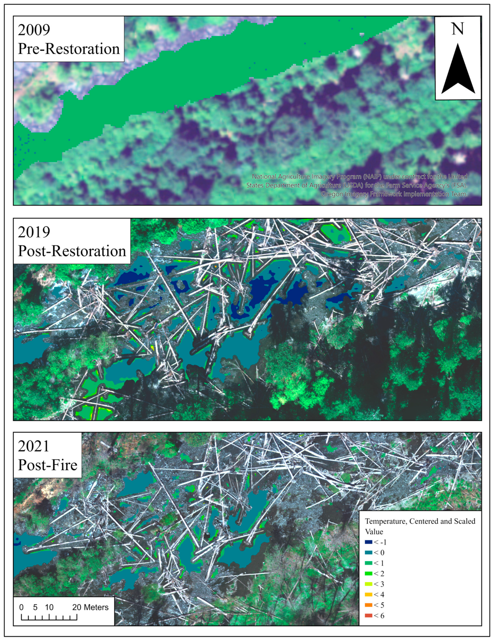
2.1. Study Area
2.2. Temperature Sensor and UAS Platform
2.3. Flight Campaigns
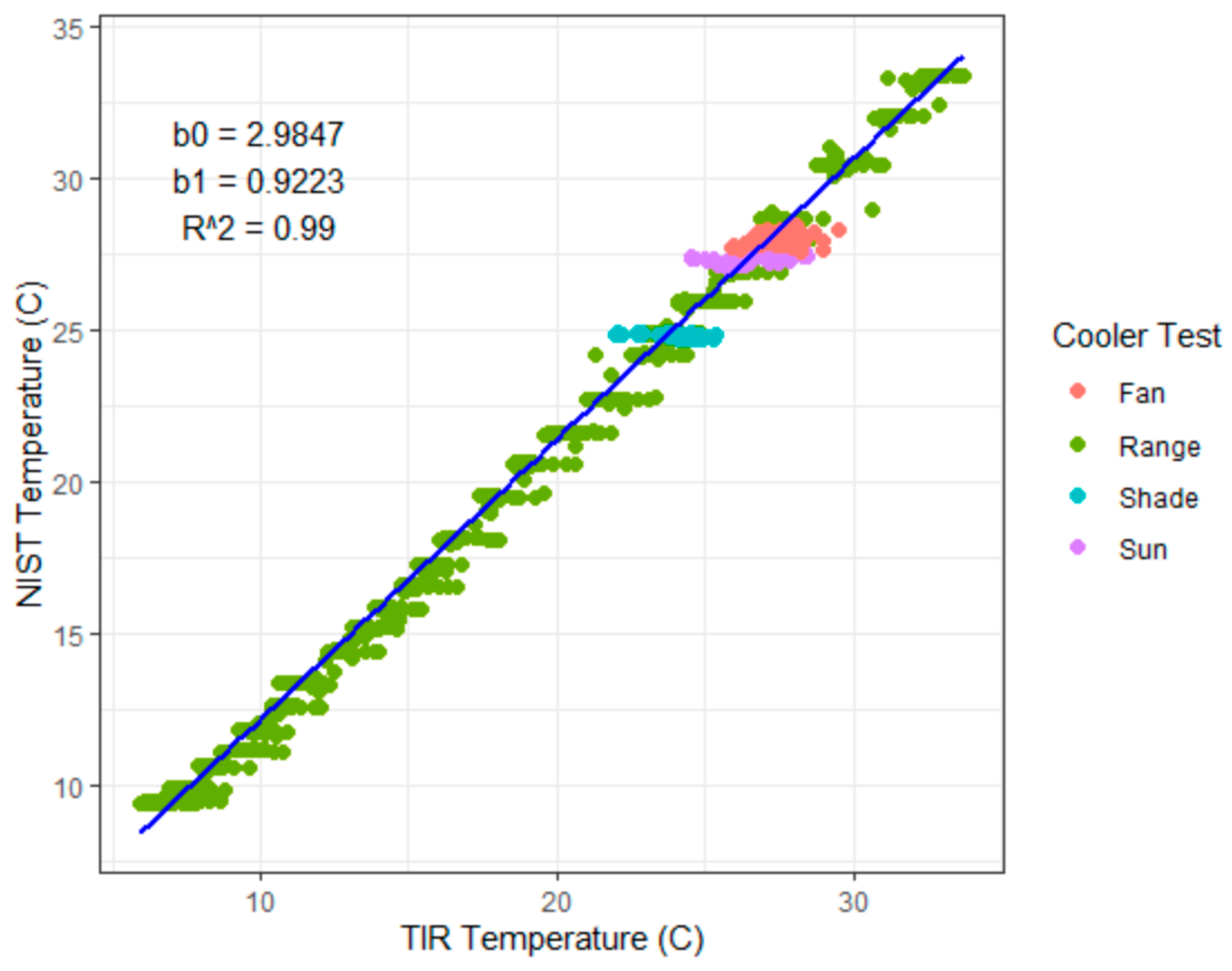
2.4. Surface Water Temperature Calibration
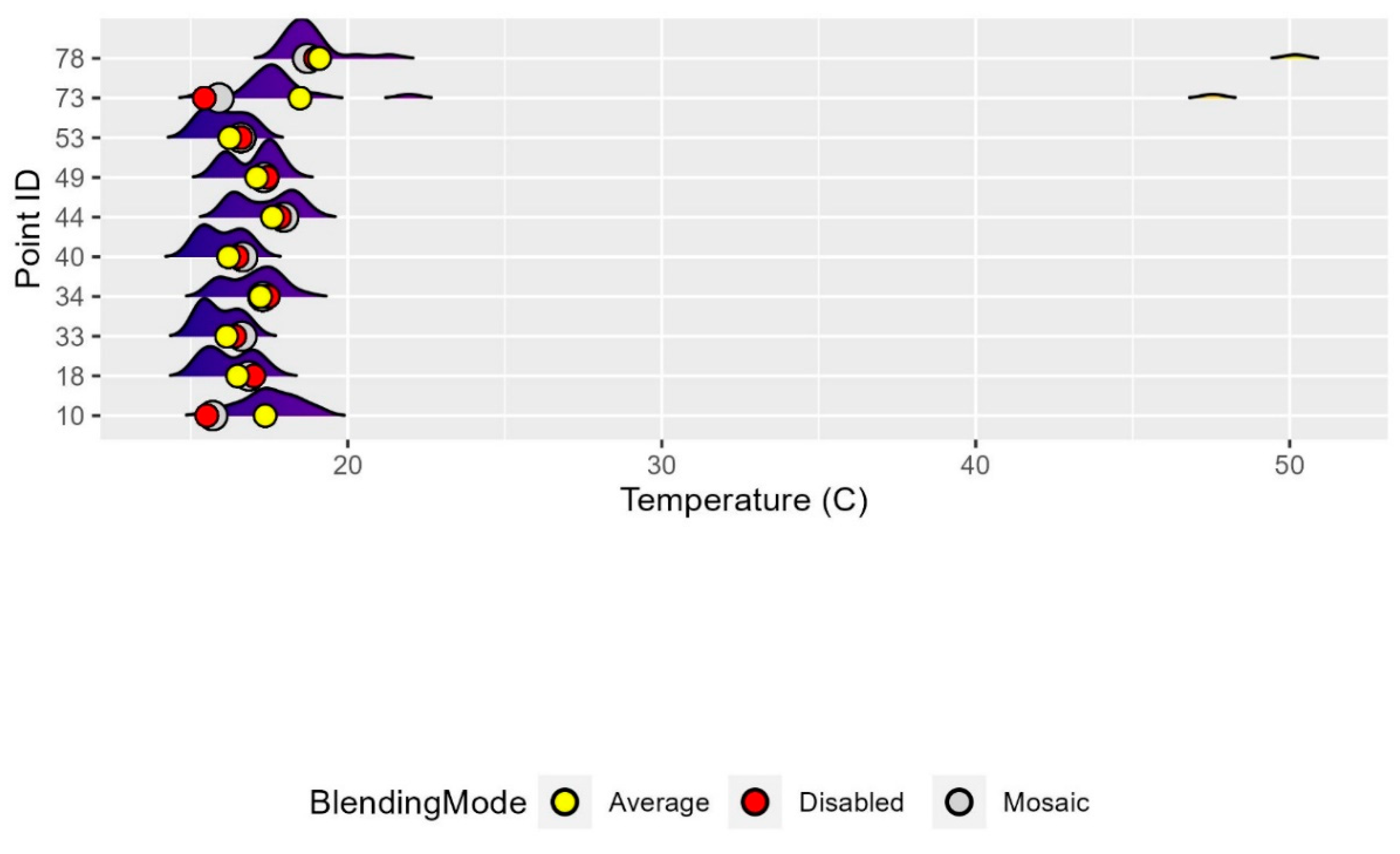
2.5. Thermal Mosaic Blending Mode Analysis
2.6. Classifying Visible Wetted Area
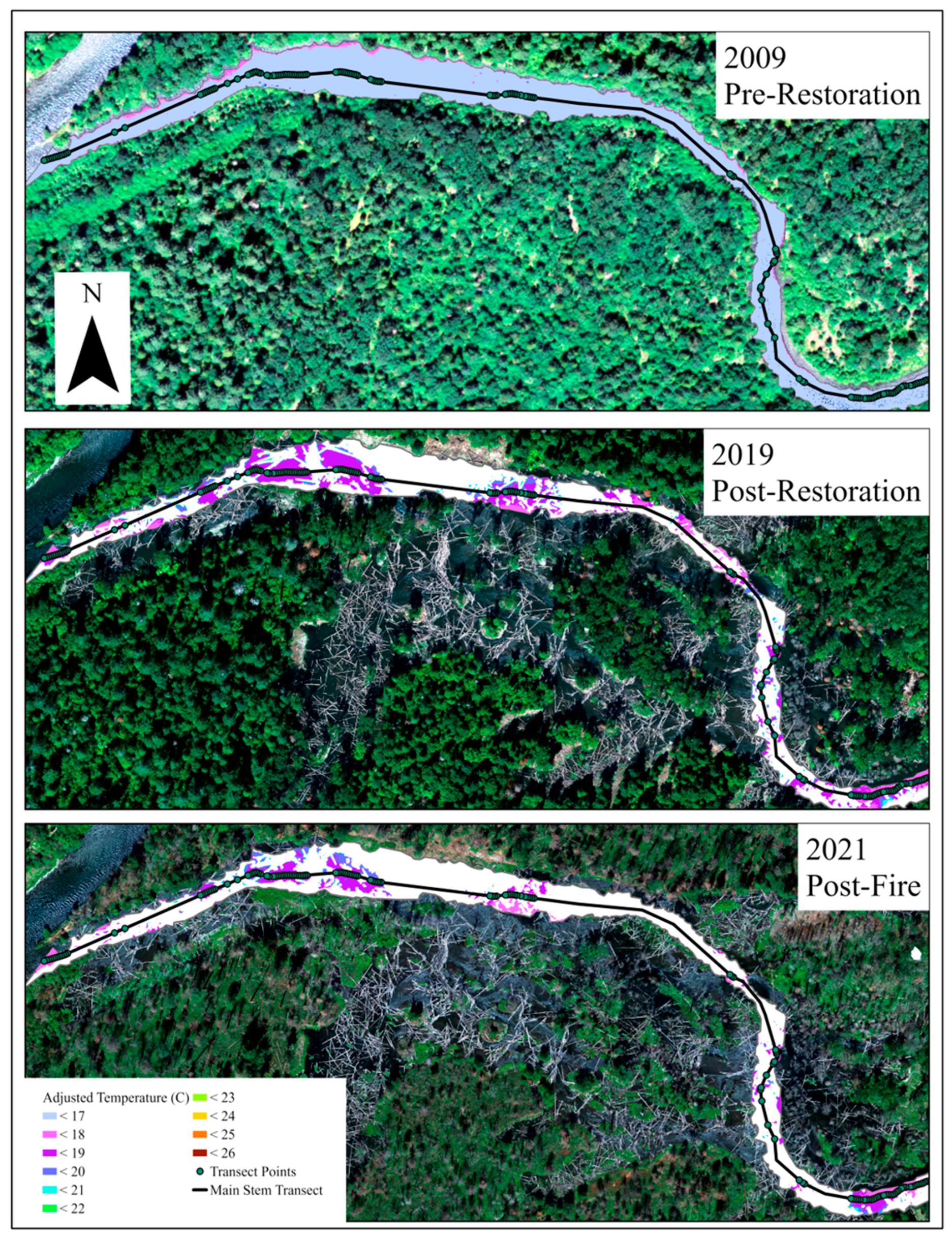
2.7. Spatiotemporal Analysis of Surface Water Temperature
2.8. Canopy Cover Analysis
2.9. Transect Analysis and Generalized Additive Model (GAM)
3. Results and Discussion
3.1. Cooler Tests and Sensor Calibration
3.2. Blending Mode Analysis
3.3. Visible Wetted Area
3.4. TIR Analysis: Global
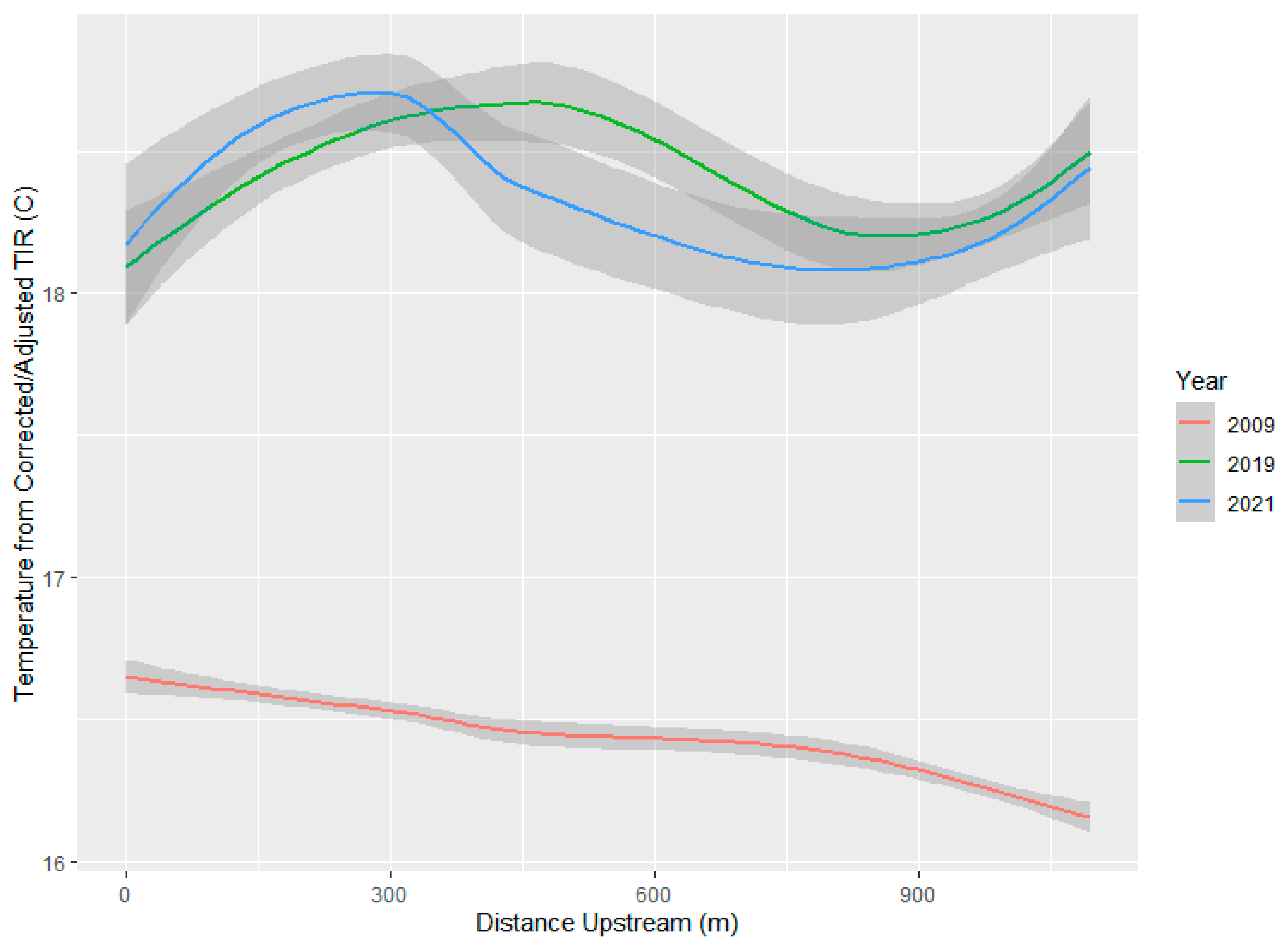
3.5. TIR Transect Analysis: Local
3.6. Generalized Additive Model for TIR Temperature
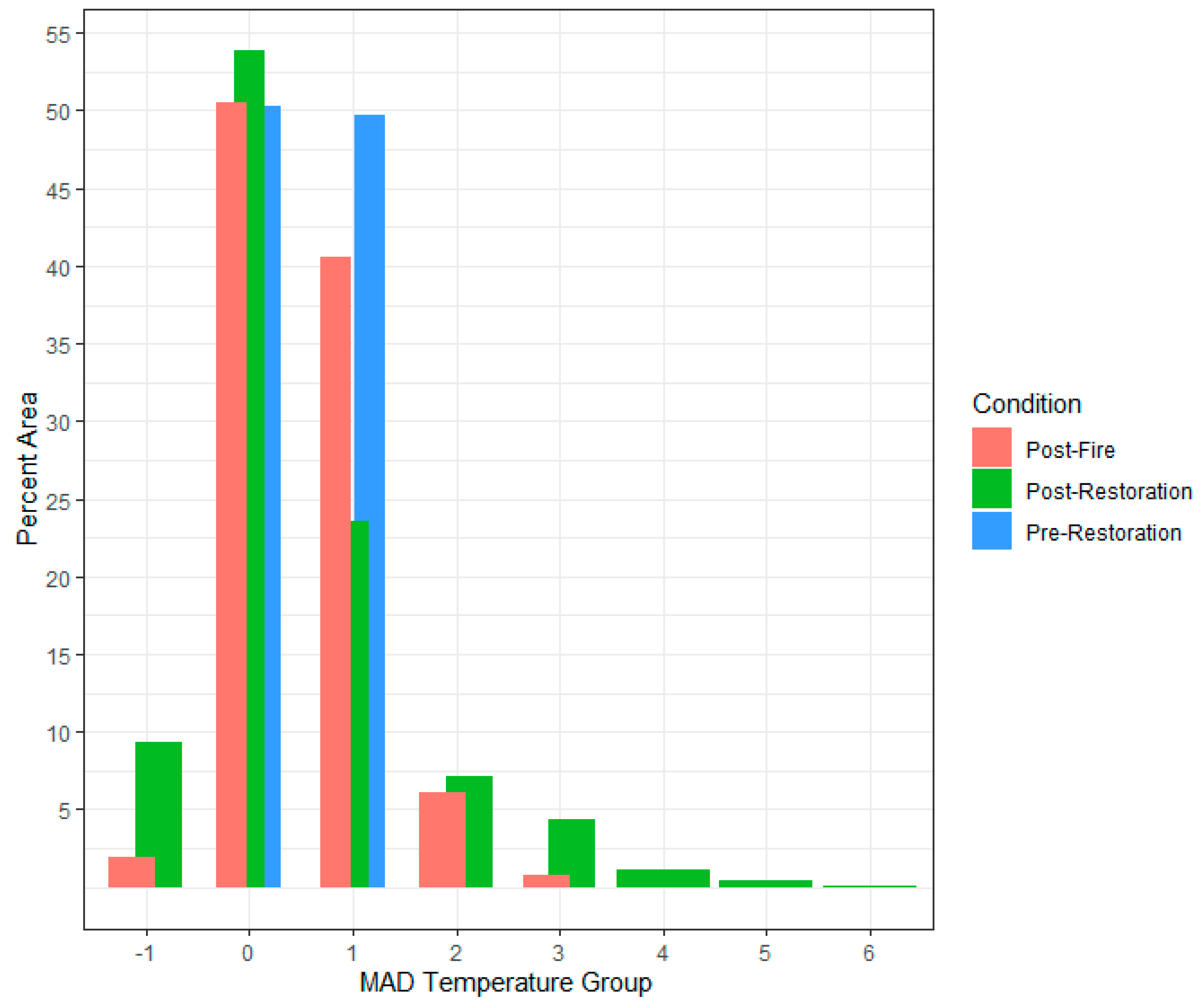
3.7. Thermal Contours and Habitat Availability
3.8. Ongoing Monitoring
4. Conclusions
Supplementary Materials
Author Contributions
Funding
Data Availability Statement
Acknowledgments
Conflicts of Interest
References
- Ward, J.V.; Stanford, J.A. Thermal Responses in the Evolutionary Ecology of Aquatic Insects. Annu. Rev. Entomol. 1982, 27, 97–117. [Google Scholar] [CrossRef]
- Holtby, L.B.; McMahon, T.E.; Scrivener, J.C. Stream Temperatures and Inter-Annual Variability in the Emigration Timing of Coho Salmon (Oncorhynchus kisutch) Smolts and fry and Chum Salmon (O. Keta) Fry from Carnation Creek, British Columbia. Can. J. Fish. Aquat. Sci. 1989, 46, 1396–1405. [Google Scholar] [CrossRef]
- Donato, M.M. A Statistical Model for Estimating Stream Temperatures in the Salmon and Clearwater River Basins, Central Idaho; US Geological Survey: Reston, VA, USA, 2002. [Google Scholar]
- McCullough, D. A Review and Synthesis of Effects of Alterations to the Water Temperature Regime on Freshwater Life Stages of Salmonids, with Special Reference to Chinook Salmon; 910-R-010; U.S. Environmental Protection Agency, Region 10: Seattle, WA, USA, 1999; p. 291. [Google Scholar]
- Houghton, J.T. Climate Change 2001: The Scientific Basis: Contribution of Working Group I to the Third Assessment Report of the Intergovernmental Panel on Climate Change; Cambridge University Press: Cambridge, UK, 2001. [Google Scholar]
- Wondzell, S.M.; Diabat, M.; Haggerty, R. What Matters Most: Are Future Stream Temperatures More Sensitive to Changing Air Temperatures, Discharge, or Riparian Vegetation? JAWRA J. Am. Water Resour. Assoc. 2019, 55, 116–132. [Google Scholar] [CrossRef]
- Wade, A.A.; Beechie, T.J.; Fleishman, E.; Mantua, N.J.; Wu, H.; Kimball, J.S.; Stoms, D.M.; Stanford, J.A. Steelhead vulnerability to climate change in the Pacific Northwest. J. Appl. Ecol. 2013, 50, 1093–1104. [Google Scholar] [CrossRef]
- Smith, D.D. Contributions of Riparian Vegetation and Stream Morphology to Headwater Stream Temperature Patterns in the Oregon Coast Range. Master’s Thesis, Oregon State University, Corvallis, OR, USA, 2004. [Google Scholar]
- Seixas, G.B.; Beechie, T.J.; Fogel, C.; Kiffney, P.M. Historical and Future Stream Temperature Change Predicted by a Lidar-Based Assessment of Riparian Condition and Channel Width. J. Am. Water Resour. Assoc. 2018, 54, 974–991. [Google Scholar] [CrossRef]
- Woltemade, C.J. Stream Temperature Spatial Variability Reflects Geomorphology, Hydrology, and Microclimate: Navarro River Watershed, California. Prof. Geogr. 2017, 69, 177–190. [Google Scholar] [CrossRef]
- Evans, E.C.; Petts, G.E. Hyporheic temperature patterns within riffles. Hydrol. Sci. J. 1997, 42, 199–213. [Google Scholar] [CrossRef]
- Wohl, E.; Lane, S.N.; Wilcox, A.C. The science and practice of river restoration. Water Resour. Res. 2015, 51, 5974–5997. [Google Scholar] [CrossRef]
- Powers, P.D.; Helstab, M.; Niezgoda, S.L. A process-based approach to restoring depositional river valleys to Stage 0, an anastomosing channel network. River Res. Appl. 2019, 35, 3–13. [Google Scholar] [CrossRef]
- Cluer, B.; Thorne, C. stream evolution model integrating habitat and ecosystem benefits. River Res. Appl. 2014, 30, 135–154. [Google Scholar] [CrossRef]
- Schumm, S.A.; Harvey, M.D.; Watson, C.C. Incised Channels: Morphology, Dynamics, and Control; Water Resources Publications: Littleton, CO, USA, 1984. [Google Scholar]
- Simon, A.; Hupp, C.R. Geomorphic and Vegetative Recovery Processes along Modified Tennessee Streams: An Interdisciplinary Approach to Disturbed Fluvial Systems. Int. Assoc. Hydrol. Sci. 1987, 167, 251–262. [Google Scholar]
- Poole, G.C.; Berman, C.H. An ecological perspective on in-stream temperature: Natural heat dynamics and mechanisms of human-caused thermal degradation. Environ. Manag. 2001, 27, 787. [Google Scholar] [CrossRef]
- Flitcroft, R.L.; Brignon, W.R.; Staab, B.; Bellmore, J.R.; Burnett, J.; Burns, P.; Cluer, B.; Giannico, G.; Helstab, J.M.; Jennings, J.; et al. Rehabilitating Valley Floors to a Stage 0 Condition: A Synthesis of Opening Outcomes. Front. Environ. Sci. 2022, 10, 892268. [Google Scholar] [CrossRef]
- Hinshaw, S.; Wohl, E.; Burnett, J.D.; Wondzell, S. Development of a geomorphic monitoring strategy for stage 0 restoration in the South Fork McKenzie River, Oregon, USA. Earth Surf. Process. Landf. 2022, 47, 1937–1951. [Google Scholar] [CrossRef]
- Fonstad, M.A.; Dietrich, J.T.; Courville, B.C.; Jensen, J.L.; Carbonneau, P.E. Topographic structure from motion: A new development in photogrammetric measurement. Earth Surf. Process. Landf. 2013, 38, 421–430. [Google Scholar] [CrossRef]
- Ireland-Otto, N.; Ciampitti, I.A.; Blanks, M.T.; Burton, R.O., Jr.; Balthazor, T. Costs of Using Unmanned Aircraft on Crop Farms. J. ASFMRA 2016, 2016, 130–148. [Google Scholar] [CrossRef]
- Torgersen, C.E.; Price, D.M.; Li, H.W.; McIntosh, B.A. Multiscale Thermal Refugia and Stream Habitat Associations of Chinook Salmon in Northeastern Oregon. Ecol. Appl. 1999, 9, 301–319. [Google Scholar] [CrossRef]
- Dugdale, S.J.; Bergeron, N.E.; St-Hilaire, A. Temporal variability of thermal refuges and water temperature patterns in an Atlantic salmon river. Remote Sens. Environ. 2013, 136, 358–373. [Google Scholar] [CrossRef]
- Dugdale, S.J. A practitioner’s guide to thermal infrared remote sensing of rivers and streams: Recent advances, precautions and considerations. Wiley Interdiscip. Rev. Water 2016, 3, 251–268. [Google Scholar] [CrossRef]
- Dugdale, S.J.; Kelleher, C.A.; Malcolm, I.A.; Caldwell, S.; Hannah, D.M. Assessing the potential of drone-based thermal infrared imagery for quantifying river temperature heterogeneity. Hydrol. Process. 2019, 33, 1152–1163. [Google Scholar] [CrossRef]
- Jensen, A.M.; Neilson, B.T.; McKee, M.; Chen, Y. Thermal remote sensing with an autonomous unmanned aerial remote sensing platform for surface stream temperatures. In Proceedings of the 2012 IEEE International Geoscience and Remote Sensing Symposium, Munich, Germany, 22–27 July 2012; pp. 5049–5052. [Google Scholar]
- Bartelt, G. Monitoring Phytoplankton Biomass and Surface Temperatures of Small Inland Lakes by Multispectral and Thermal UAS Imagery. Master’s Thesis, University of Minnesota, Minneapolis, MN, USA, 2021. [Google Scholar]
- Tunca, E.; Köksal, E.S.; Çetin Taner, S. Calibrating UAV thermal sensors using machine learning methods for improved accuracy in agricultural applications. Infrared Phys. Technol. 2023, 133, 104804. [Google Scholar] [CrossRef]
- Niwa, H. Comparison of the accuracy of two UAV-mounted uncooled thermal infrared sensors in predicting river water temperature. River Res. Appl. 2022, 38, 1660–1667. [Google Scholar] [CrossRef]
- Boyd, M.; Kasper, B. Analytical Methods for Dynamic Open Channel Heat and Mass Transfer: Methodology for the Heat Source Model Version 7.0; Watershed Sciences, Inc.: Portland, OR, USA, 2003. [Google Scholar]
- Woltemade, C.J.; Hawkins, T.W. Stream Temperature Impacts Because of Changes in Air Temperature, Land Cover and Stream Discharge: Navarro River Watershed, California, USA. River Res. Appl. 2016, 32, 2020–2031. [Google Scholar] [CrossRef]
- Franklin, J.F.; Dryness, C.T. Natural Vegetation of Oregon and Washington; U.S.D.A. Forest Service: Portland, OR, USA, 1973. [Google Scholar]
- Geist, D.R.; Dauble, D.D. Redd Site Selection and Spawning Habitat Use by Fall Chinook Salmon: The Importance of Geomorphic Features in Large Rivers. Environ. Manag. 1998, 22, 655–669. [Google Scholar] [CrossRef]
- McHugh, P.; Budy, P. Patterns of Spawning Habitat Selection and Suitability for Two Populations of Spring Chinook Salmon, with an Evaluation of Generic versus Site-Specific Suitability Criteria. Trans. Am. Fish. Soc. 2004, 133, 89–97. [Google Scholar] [CrossRef]
- Reiser, D.W.; White, R.G. Effects of Two Sediment Size-Classes on Survival of Steelhead and Chinook Salmon Eggs. N. Am. J. Fish. Manag. 1988, 8, 432–437. [Google Scholar] [CrossRef]
- McKenzie Watershed Council. Phase I Summary. Available online: https://www.mckenziewc.org/phase-1-2/ (accessed on 13 February 2024).
- MicaSense. MicaSense Altum and DLS 2 Integration Guide; MicaSense: Seattle, WA, USA, 2020. [Google Scholar]
- DJI. DJI Pilot—DJI Download Center—DJI. Available online: https://www.dji.com/downloads/djiapp/dji-pilot (accessed on 19 May 2020).
- Agisoft. Agisoft Metashape. Available online: https://www.agisoft.com/pdf/metashape-pro_2_1_en.pdf (accessed on 18 May 2020).
- Watershed Sciences. Airborne Thermal Infrared Remote Sensing McKenzie River Basin, Oregon; Watershed Sciences: Corvallis, OR, USA, 2009. [Google Scholar]
- U.S. Geological Survey. National Water Information System Data Available on the World Wide Web (Water Data for the Nation). Available online: https://nwis.waterdata.usgs.gov/nwis/uv?cb_00010=on&format=html&site_no=14159500&legacy=1&period=&begin_date=2021-07-15&end_date=2021-07-15 (accessed on 13 February 2024).
- Jensen, A.M.; McKee, M.; Chen, Y. Procedures for processing thermal images using low-cost microbolometer cameras for small unmanned aerial systems. In Proceedings of the 2014 IEEE Geoscience and Remote Sensing Symposium, Quebec City, QC, Canada, 13–18 July 2014; pp. 2629–2632. [Google Scholar]
- Abolt, C.; Caldwell, T.; Wolaver, B.; Pai, H. Unmanned aerial vehicle-based monitoring of groundwater inputs to surface waters using an economical thermal infrared camera. Opt. Eng. 2018, 57, 1. [Google Scholar] [CrossRef]
- RBR Global. RBRsolo3 T Datasheet. Available online: https://rbr-global.com/wp-content/uploads/2023/12/RBRsolo3-T-Datasheet-0005583revG.pdf (accessed on 1 December 2023).
- Ribeiro-Gomes, K.; Hernández-López, D.; Ortega, J.F.; Ballesteros, R.; Poblete, T.; Moreno, M.A. Uncooled Thermal Camera Calibration and Optimization of the Photogrammetry Process for UAV Applications in Agriculture. Sensors 2017, 17, 2173. [Google Scholar] [CrossRef]
- Malbeteau, Y.; Johansen, K.; Aragon, B.; Al-Mashhawari, S.K.; McCabe, M.F. Overcoming the Challenges of Thermal Infrared Orthomosaics Using a Swath-Based Approach to Correct for Dynamic Temperature and Wind Effects. Remote Sens. 2021, 13, 3255. [Google Scholar] [CrossRef]
- Acorsi, M.G.; Gimenez, L.M.; Martello, M. Assessing the Performance of a Low-Cost Thermal Camera in Proximal and Aerial Conditions. Remote Sens. 2020, 12, 3591. [Google Scholar] [CrossRef]
- Esri. ArcGIS Pro, 2.8.2; Esri Inc.: Redlands, CA, USA, 2021.
- McFeeters, S.K. The use of the Normalized Difference Water Index (NDWI) in the delineation of open water features. Int. J. Remote Sens. 1996, 17, 1425–1432. [Google Scholar] [CrossRef]
- McFeeters, S. Using the Normalized Difference Water Index (NDWI) within a Geographic Information System to Detect Swimming Pools for Mosquito Abatement: A Practical Approach. Remote Sens. 2013, 5, 3544–3561. [Google Scholar] [CrossRef]
- Rees, G. Physical Principles of Remote Sensing, 3rd ed.; Cambridge University Press: Cambridge, UK, 2013. [Google Scholar]
- Cherkauer, K.A.; Burges, S.J.; Handcock, R.N.; Kay, J.E.; Kampf, S.K.; Gillespie, A.R. Assessing Satllite-Based and Aircraft-Based thermal Infrared Remote Sensing for Monitoring Pacific Northwest River Temperature. JAWRA J. Am. Water Resour. Assoc. 2005, 41, 1149–1159. [Google Scholar] [CrossRef]
- Roussel, J.R.; Auty, D. Airborne LiDAR Data Manipulation and Visualization for Forestry Applications, R package version 3.1.1; r-lidar: Québec, QC, Canada, 2021.
- R Core Team. R: A Language and Environment for Statistical Computing, 4.1.2; R Core Team: Vienna, Austria, 2021.
- Zhang, W.; Qi, J.; Wan, P.; Wang, H.; Xie, D.; Wang, X.; Yan, G. An Easy-to-Use Airborne LiDAR Data Filtering Method Based on Cloth Simulation. Remote Sens. 2016, 8, 501. [Google Scholar] [CrossRef]
- Rouse, J.W., Jr.; Haas, R.H.; Schell, J.A.; Deering, D.W. Monitoring Vegetation Systems in the Great Plains with Erts. 1974, Volume 351, p. 309. Available online: https://api.semanticscholar.org/CorpusID:133358670 (accessed on 16 September 2020).
- Lillesand, T.M.; Kiefer, R.W.; Chipman, J.W. Remote Sensing and Image Interpretation, 7th ed.; Hoboken, N.J., Ed.; John Wiley & Sons, Inc.: Hoboken, NJ, USA, 2015. [Google Scholar]
- Hijmans, R.J. Raster: Geographic Data Analysis and Modeling; R package version 3.5-9. Available online: https://cran.r-project.org/web/packages/raster/index.html (accessed on 20 December 2021).
- Forest Accord Signatories. Oregon Private Forest Accord; Oregon Department of Forestry: Salem, OR, USA, 2022. [Google Scholar]
- Wood, S.N. Generalized Additive Models: An Introduction with R, 2nd ed.; Chapman and Hall/CRC: Boca Raton, FL, USA, 2017. [Google Scholar]
- Ebert, L.A.; Talib, A.; Zipper, S.C.; Desai, A.R.; Paw, U.K.T.; Chisholm, A.J.; Prater, J.; Nocco, M.A. How High to Fly? Mapping Evapotranspiration from Remotely Piloted Aircrafts at Different Elevations. Remote Sens. 2022, 14, 1660. [Google Scholar] [CrossRef]
- Minkina, W.; Klecha, D. Atmospheric transmission coefficient modelling in the infrared for thermovision measurements. J. Sens. Sens. Syst. 2016, 5, 17–23. [Google Scholar] [CrossRef]
- Barker, M.I.; Burnett, J.D.; Gutiérrez, F.M.; Wondzell, S.M.; Wing, M.G. Sampling-Based Approaches to Estimating Two-Dimensional Large Wood Area from UAS Imagery. J. Geogr. Inf. Syst. 2022, 14, 571–588. [Google Scholar] [CrossRef]
- Johnson, S.L.; Jones, J.A. Stream temperature responses to forest harvest and debris flows in western Cascades, Oregon. Can. J. Fish. Aquat. Sci. 2000, 57, 30–39. [Google Scholar] [CrossRef]
- D’Souza, L.E.; Reiter, M.; Six, L.J.; Bilby, R.E. Response of vegetation, shade and stream temperature to debris torrents in two western Oregon watersheds. For. Ecol. Manag. 2011, 261, 2157–2167. [Google Scholar] [CrossRef]
- Brown, G.W. Predicting Temperatures of Small Streams. Water Resour. Res. 1969, 5, 68–75. [Google Scholar] [CrossRef]
- Berman, C.H.; Quinn, T.P. Behavioural thermoregulation and homing by spring chinook salmon, Oncorhynchus tshawytscha (Walbaum), in the Yakima River. J. Fish Biol. 1991, 39, 301–312. [Google Scholar] [CrossRef]
- Armstrong, J.B.; Fullerton, A.H.; Jordan, C.E.; Ebersole, J.L.; Bellmore, J.R.; Arismendi, I.; Penaluna, B.; Reeves, G.H. The importance of warm habitat to the growth regime of cold-water fishes. Nat. Clim. Chang. 2021, 11, 354–361. [Google Scholar] [CrossRef]
- Isaak, D.J.; Young, M.K.; Nagel, D.E.; Horan, D.L.; Groce, M.C. The cold-water climate shield: Delineating refugia for preserving salmonid fishes through the 21st century. Glob. Change Biol. 2015, 21, 2540–2553. [Google Scholar] [CrossRef]
- Ruff, C.P.; Schindler, D.E.; Armstrong, J.B.; Bentley, K.T.; Brooks, G.T.; Holtgrieve, G.W.; McGlauflin, M.T.; Torgersen, C.E.; Seeb, J.E. Temperature-associated population diversity in salmon confers benefits to mobile consumers. Ecology 2011, 92, 2073–2084. [Google Scholar] [CrossRef]
- Ebersole, J.L.; Liss, W.J.; Frissell, C.A. Thermal heterogeneity, stream channel morphology, and salmonid abundance in northeastern Oregon streams. Can. J. Fish. Aquat. Sci. 2003, 60, 1266–1280. [Google Scholar] [CrossRef]


| Flight | Condition | Time UTC (−7 for PDT) | Thermal Sensor | Air Temp. (°C) | Ground Sampling Distance (cm) | Discharge (m3/s) | Water Temp at Release (°C) |
|---|---|---|---|---|---|---|---|
| 22 August 2009 | Pre-restoration | 19:00–20:00 | FLIR System SC6000 | 26.7 | 43 | 14.5 | 15.1 |
| 26 August 2019 | Post-restoration | 20:14–21:17 | Micasense Altum | 28.9 | 101 | 23.4 | 14–14.3 |
| 27 August 2019 | Post-restoration | 20:44–21:10 | Micasense Altum | 36.1 | 101 | 23.4 | 14.7 |
| 15 July 2021 | Post-restoration, post-fire | 19:40–21:12 | Micasense Altum | 27.2 | 101 | 11.0 | 15.3 |
| Treatment | Range (Uncorrected TIR, NIST) | Mean (Uncorrected TIR, NIST) | Mean (Corrected TIR) | Uncorrected Error Range | N | 10 rep 10-Fold CV RMSE, MAE (Uncorrected) | 10 rep 10-Fold CV RMSE, MAE (Corrected) |
|---|---|---|---|---|---|---|---|
| Shade | 22.0–25.3, 24.7–25.0 | 24.1, 24.8 | 25.2 | −2.9–0.6 | 60 | 1.08, 0.74 | 0.89, 0.80 |
| Sun | 24.5–28.5, 27.1–27.8 | 26.6, 27.4 | 27.6 | −2.9–1.1 | 62 | 1.17, 0.93 | 0.81, 0.64 |
| Fan | 25.9–29.5, 27.6–28.4 | 27.6, 28.0 | 28.4 | −1.9–1.3 | 65 | 0.85, 0.68 | 0.81, 0.66 |
| Range | 6.0–33.7, 9.5–33.4 | 16.9, 18.6 | 18.6 | −3.5–1.7 | 1741 | 1.84, 1.71 | 0.42, 0.31 |
| All Data | 5.97–33.68, 9.47–33.39 | 17.83, 19.43 | 19.4 | −3.5–1.7 | 1928 | 1.78, 1.62 | 0.48, 0.35 |
| Uncorrected Temperature Data (Celsius) | |||||
|---|---|---|---|---|---|
| Dataset | N Cells | Range | 1st, 99th Percentiles | Mean | Standard Deviation |
| 22 August 2009 | 74,632 | 16.9–23.4 | 17.0, 18.3 | 17.5 | 0.3 |
| 26 August 2019 | 6,673,200 | 12.0–38.4 | 15.2, 24.7 | 17.5 | 1.8 |
| 15 July 2021 | 2,396,912 | 16.0–34.0 | 16.6, 21.8 | 18.3 | 1.1 |
| Corrected and Gage-Adjusted Temperature Data filtered from 1st to 99th Percentiles (Celsius) | |||||
| Dataset | N Cells (NA ignored) | Range | 1st, 99th Percentiles | Mean | Standard Deviation |
| 22 August 2009 * | 72,483 | 16.2–17.3 | 16.2, 17.2 | 16.5 | 0.2 |
| 26 August 2019 | 6,538,900 | 17.0–25.7 | 17.2, 23.5 | 19.1 | 1.3 ** |
| 15 July 2021 | 2,348,018 | 17.1–21.9 | 17.3, 21.1 | 18.7 | 0.8 |
| Year | Min | Max | Mean | Median | MAD |
|---|---|---|---|---|---|
| 2009 | 16.15 | 16.95 | 16.43 | 16.45 | 0.297 |
| 2019 | 17.61 | 19.89 | 18.41 | 18.37 | 0.458 |
| 2021 | 17.31 | 20.82 | 18.41 | 18.25 | 0.677 |
| Parametric Coefficients | ||
|---|---|---|
| Variable | Est. Coefficient | p-Value |
| Intercept | 0 | N/A |
| Discharge (m3/s) | −0.4 | <0.001 |
| Percent Canopy Cover (0–1) | −2.2 | <0.001 |
| Air Temperature (°C) | 0.7 | <0.001 |
| Smooth Terms | ||
| Smooth term | Est. Degrees of Freedom (EDF) | p-value |
| Year (random effect penalty) | ~0.0 | <0.001 |
| Distance Upstream (m) | 1.0 | 0.005 |
| Location (Longitude, Latitude) | 2.0 | 0.008 |
| Tensor Product interaction (Location × Distance Upstream) | 6.8 | <0.001 |
| Total Area of Wetted Cells in Temperature Deviation Groups (m2) | ||||||||
|---|---|---|---|---|---|---|---|---|
| Year | −1 | 0 | 1 | 2 | 3 | 4 | 5 | 6 |
| 2009 | NA | 13,111 | 12,983 | NA | NA | NA | NA | NA |
| 2019 | 2273 | 13,175 | 5775 | 1744 | 1080 | 279 | 118 | 16 |
| 2021 | 240 | 6121 | 4913 | 743 | 91 | NA | NA | NA |
Disclaimer/Publisher’s Note: The statements, opinions and data contained in all publications are solely those of the individual author(s) and contributor(s) and not of MDPI and/or the editor(s). MDPI and/or the editor(s) disclaim responsibility for any injury to people or property resulting from any ideas, methods, instructions or products referred to in the content. |
© 2025 by the authors. Licensee MDPI, Basel, Switzerland. This article is an open access article distributed under the terms and conditions of the Creative Commons Attribution (CC BY) license (https://creativecommons.org/licenses/by/4.0/).
Share and Cite
Barker, M.I.; Burnett, J.D.; Arismendi, I.; Wing, M.G. Assessing Heterogeneity of Surface Water Temperature Following Stream Restoration and a High-Intensity Fire from Thermal Imagery. Remote Sens. 2025, 17, 1254. https://doi.org/10.3390/rs17071254
Barker MI, Burnett JD, Arismendi I, Wing MG. Assessing Heterogeneity of Surface Water Temperature Following Stream Restoration and a High-Intensity Fire from Thermal Imagery. Remote Sensing. 2025; 17(7):1254. https://doi.org/10.3390/rs17071254
Chicago/Turabian StyleBarker, Matthew I., Jonathan D. Burnett, Ivan Arismendi, and Michael G. Wing. 2025. "Assessing Heterogeneity of Surface Water Temperature Following Stream Restoration and a High-Intensity Fire from Thermal Imagery" Remote Sensing 17, no. 7: 1254. https://doi.org/10.3390/rs17071254
APA StyleBarker, M. I., Burnett, J. D., Arismendi, I., & Wing, M. G. (2025). Assessing Heterogeneity of Surface Water Temperature Following Stream Restoration and a High-Intensity Fire from Thermal Imagery. Remote Sensing, 17(7), 1254. https://doi.org/10.3390/rs17071254