
The Predictive Skill of a Remote Sensing-Based Machine Learning Model for Ice Wedge and Visible Ground Ice Identification in Western Arctic Canada


Abstract
1. Introduction
2. Methods
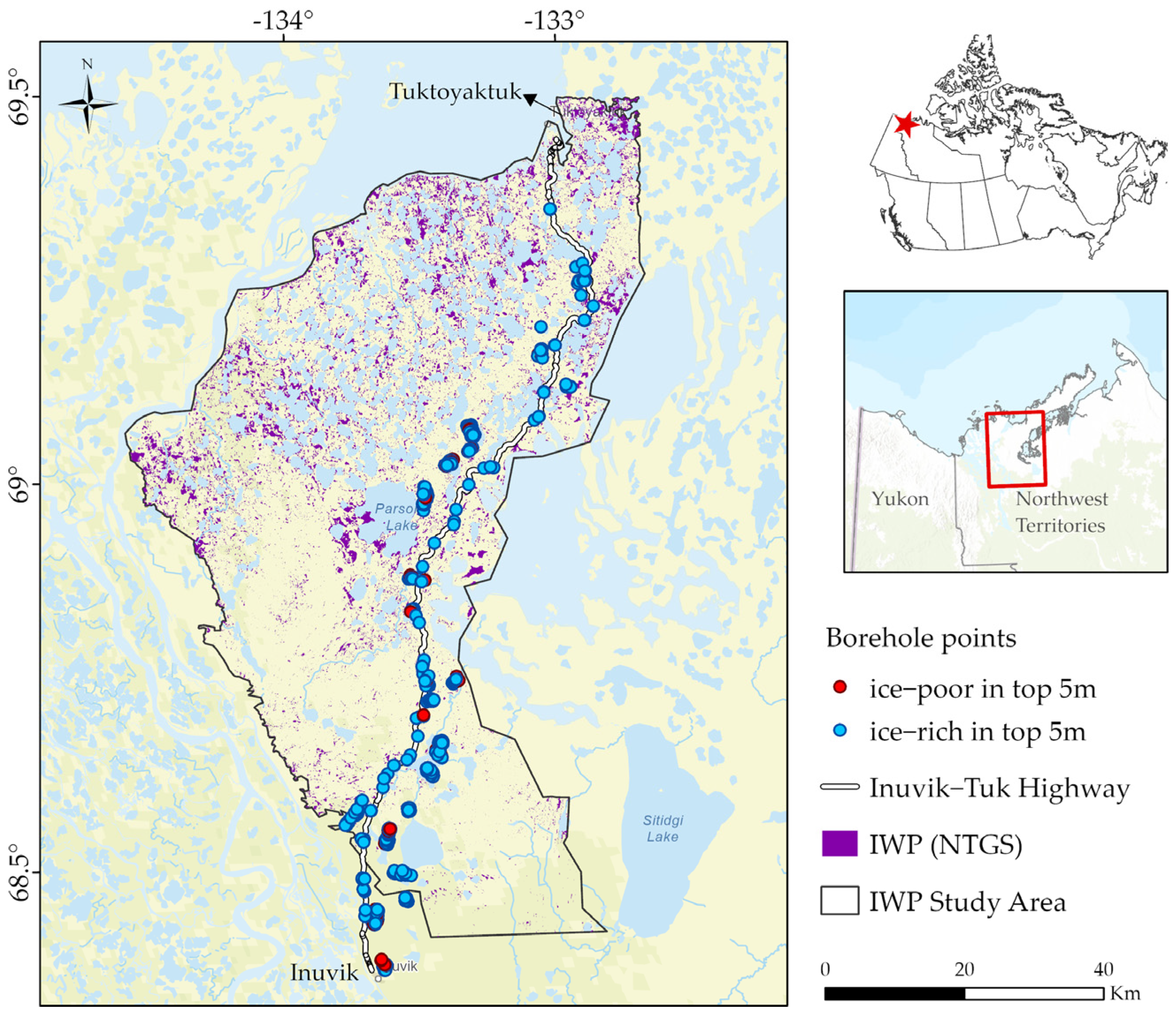
2.1. Study Area
2.2. Reference Data
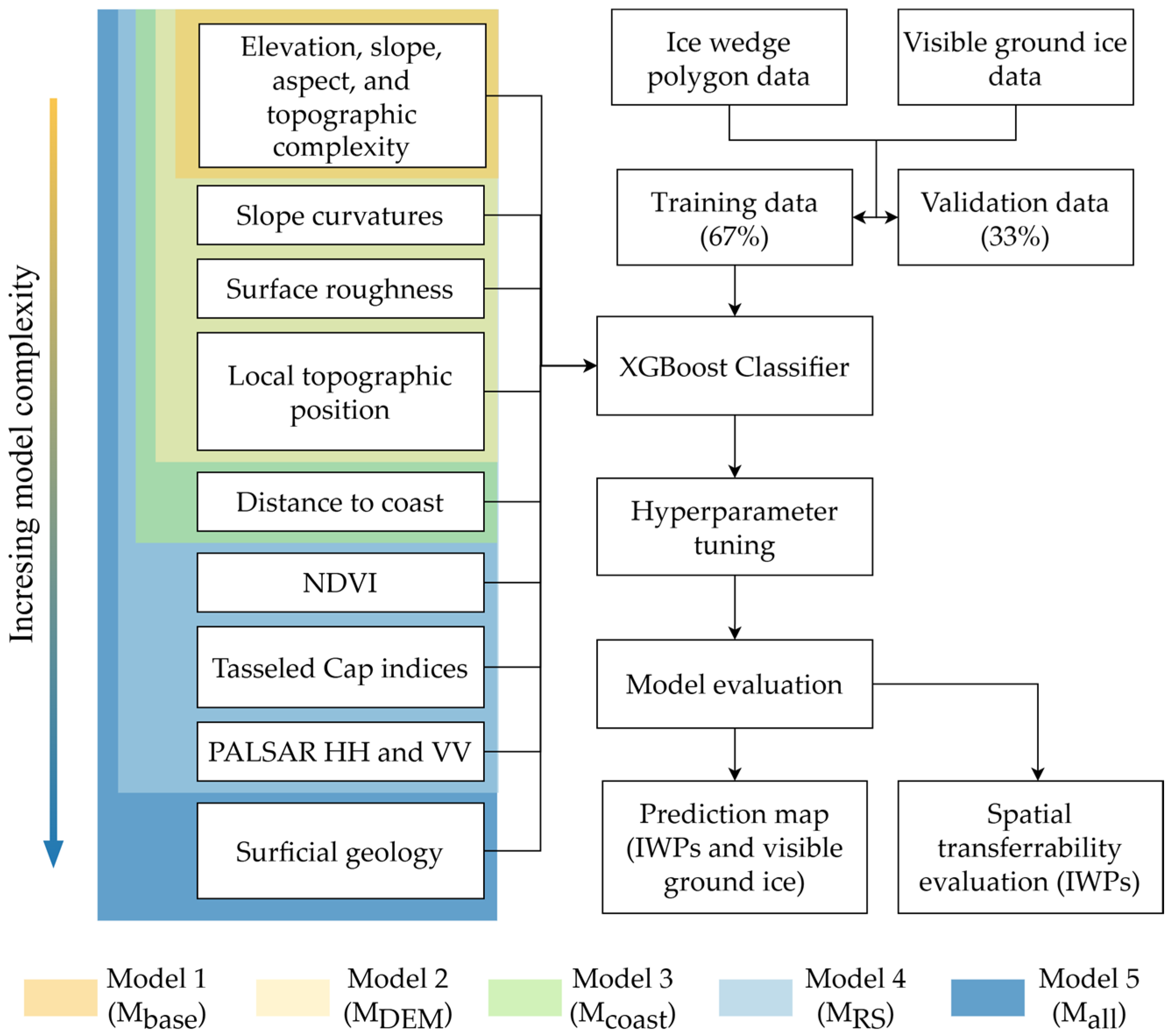
2.3. Predictor Variables
2.4. Training and Evaluation
2.4.1. Prediction Model
2.4.2. Model Training
2.4.3. Model Evaluation
3. Results
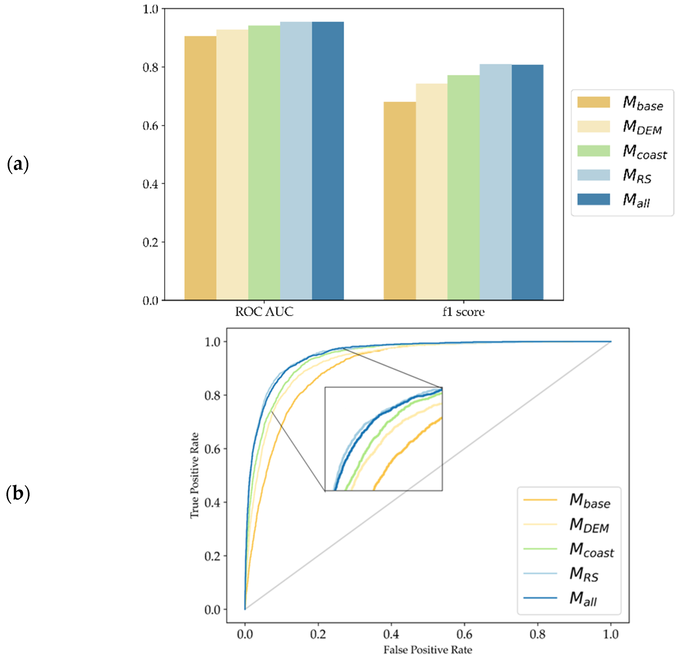
3.1. IWP Model Predictive Skill
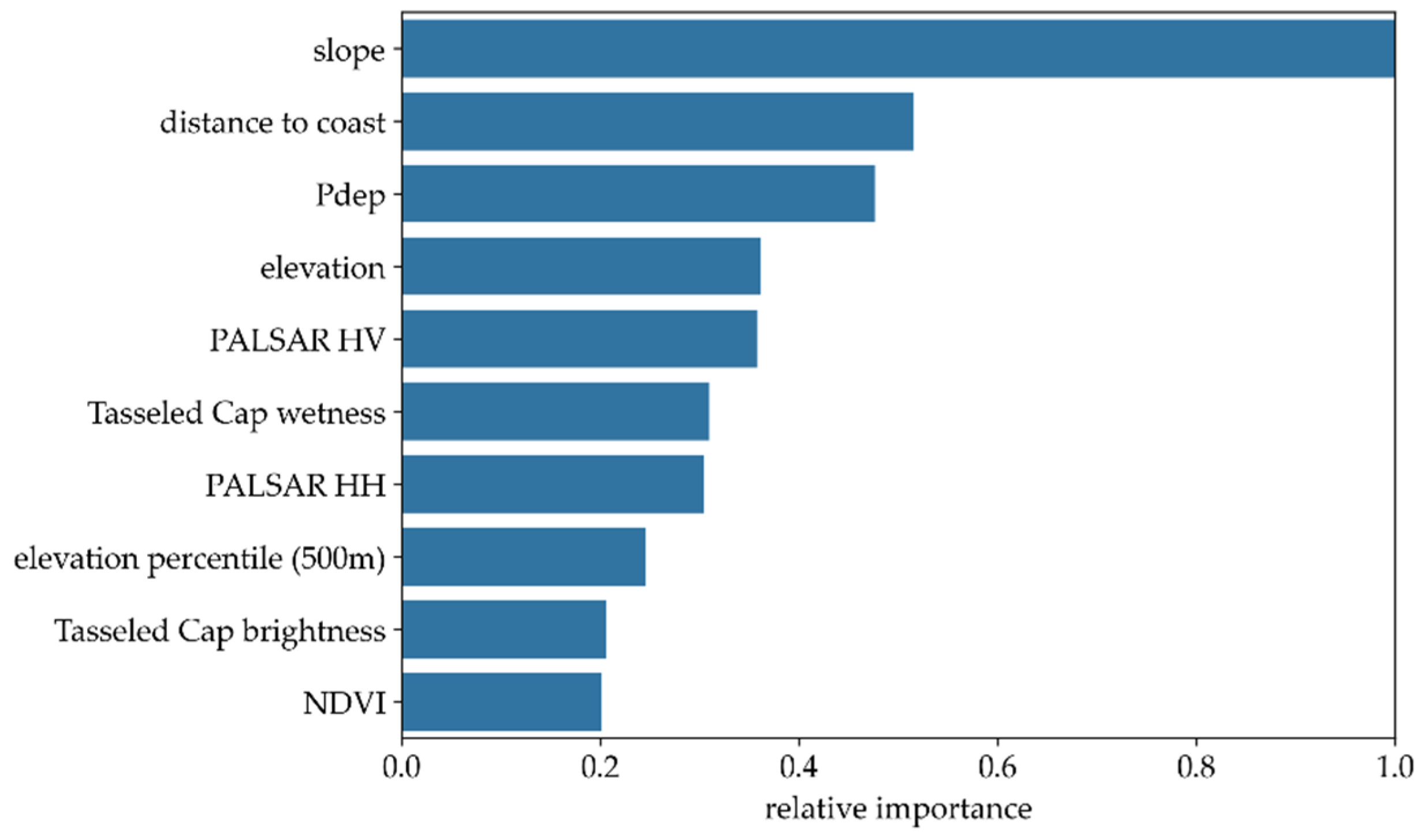
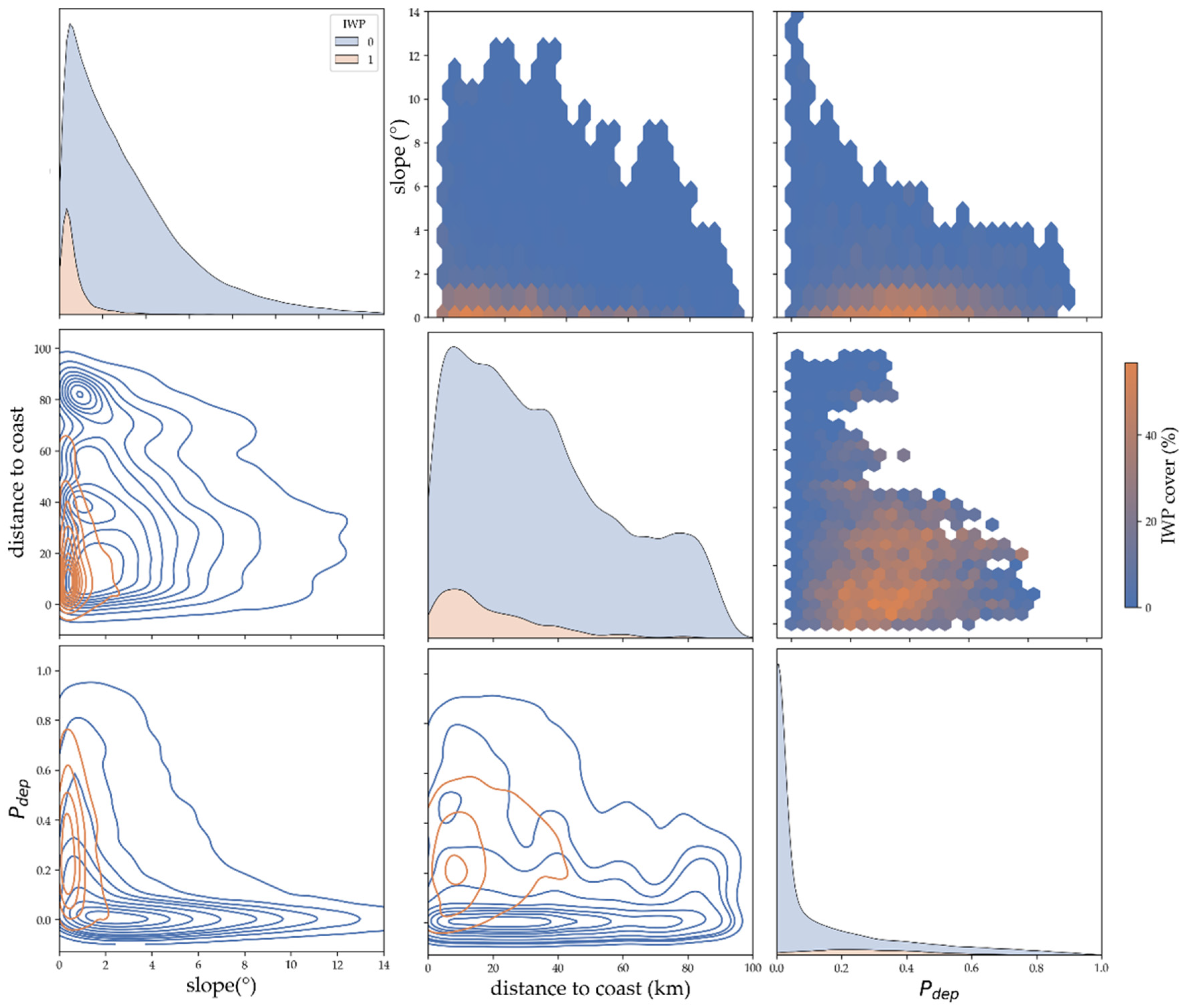
3.2. IWP Variable Importance
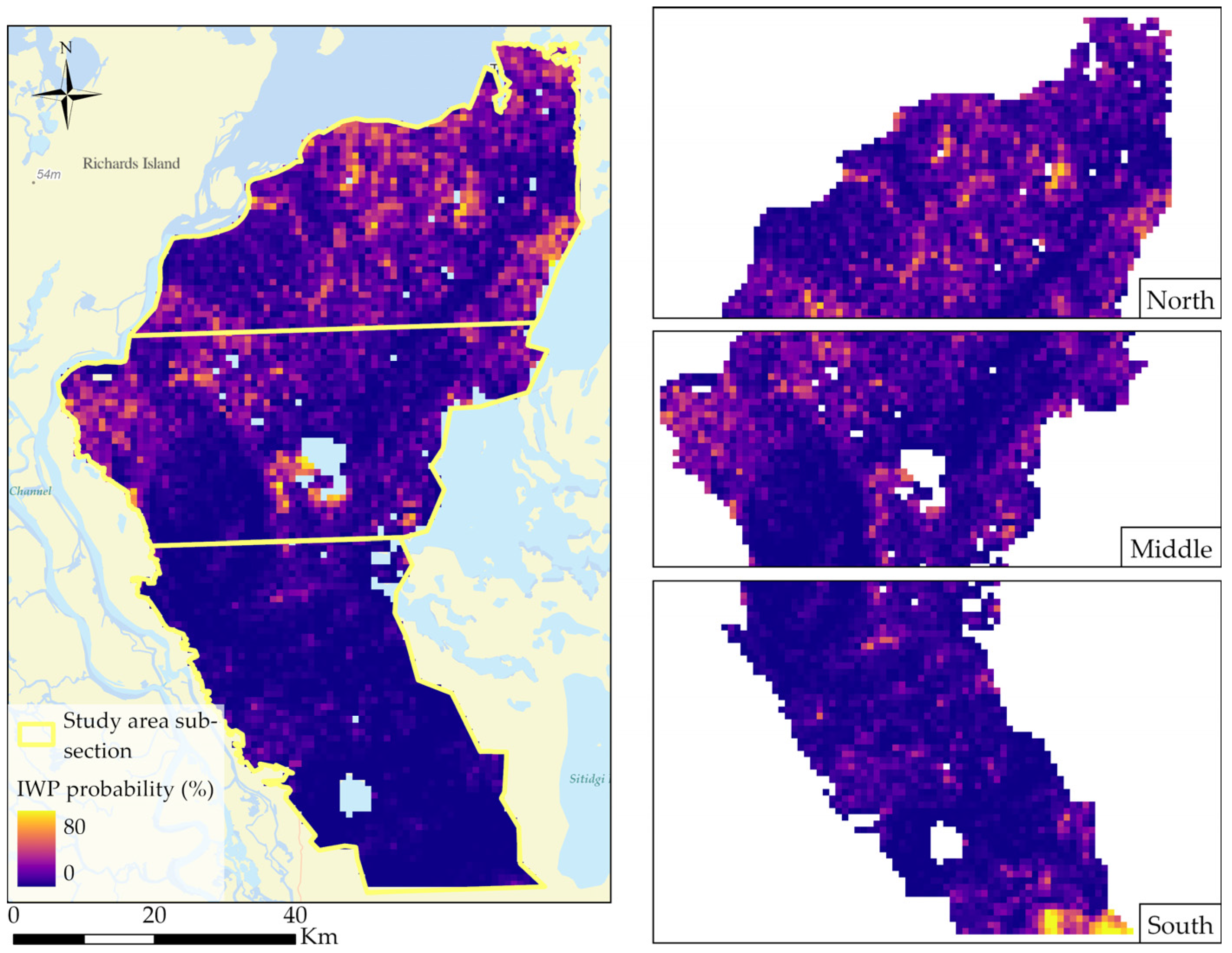
3.3. Map of Predicted IWP Probability
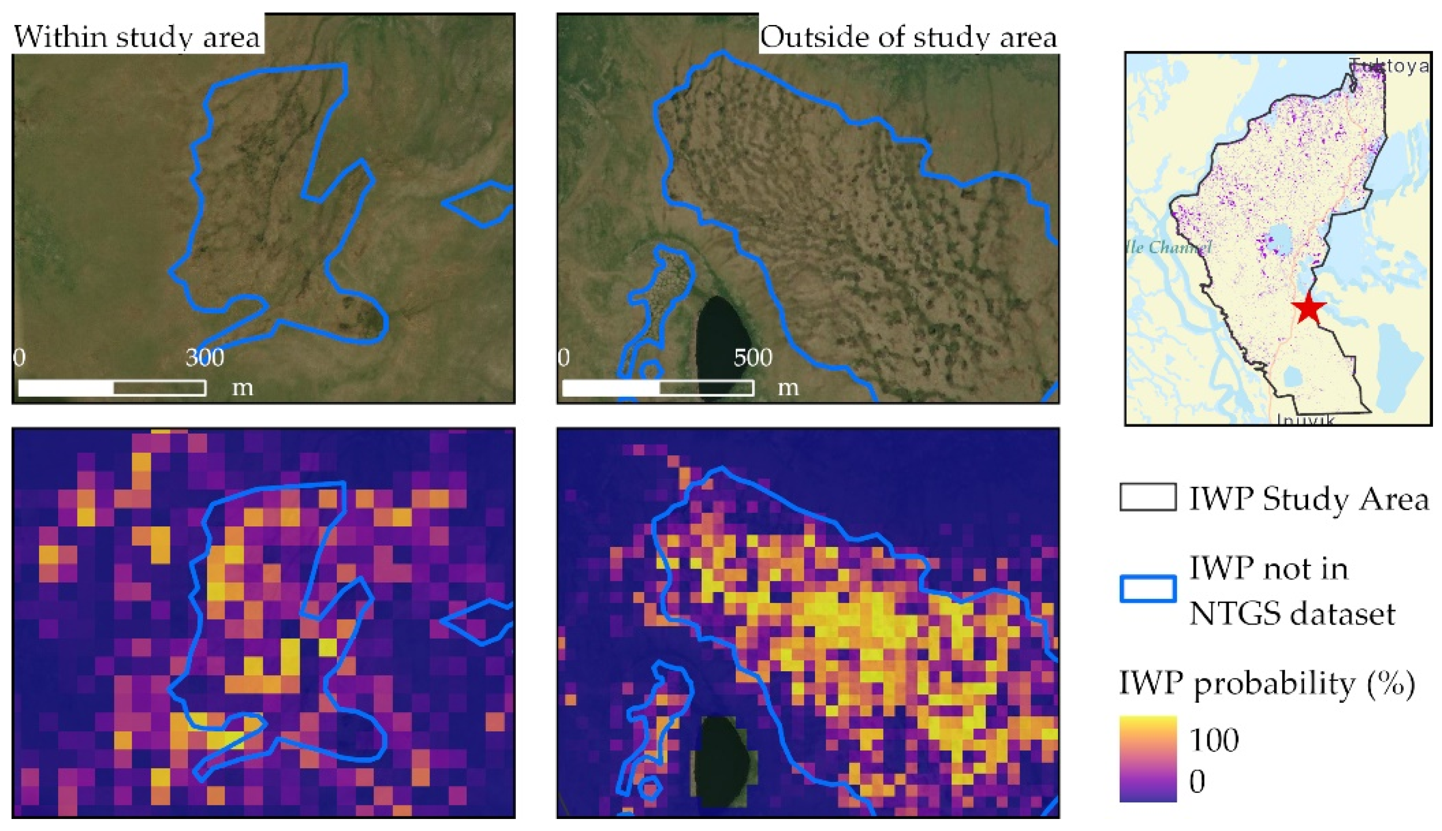
3.4. Spatial Transferability of IWP Model
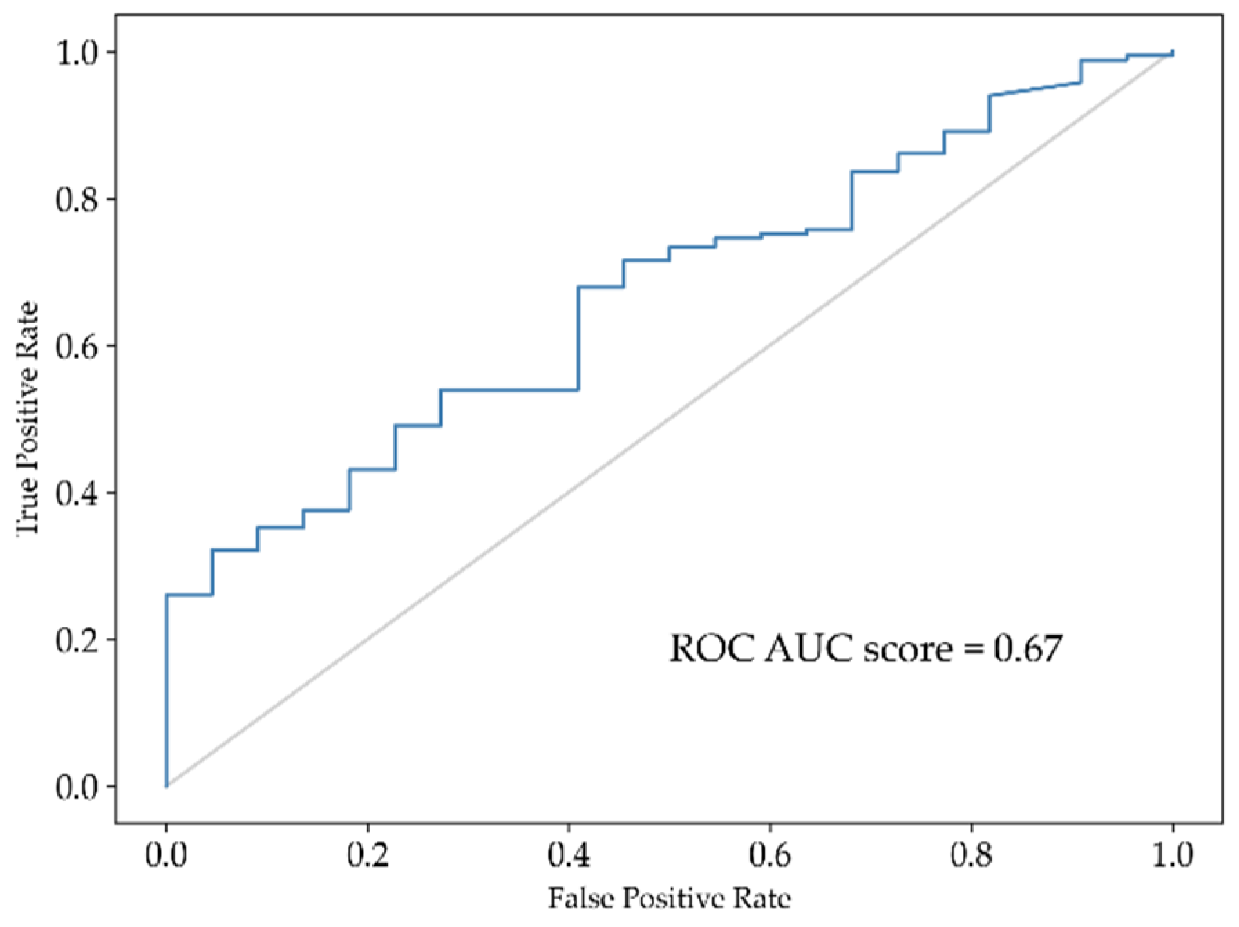
3.5. Visible Ground Ice Model
4. Discussion
4.1. Predictive Skill
4.2. Improving Ground Ice Maps and Process Understanding
5. Conclusions
- We found a high predictability of IWPs from topographic and remote sensing attributes with a ROC AUC and macro F1 score of 0.95 and 0.80 for MRS. The most important predictors were slope, distance to the coast, and probability of depression.
- The model accurately predicted regional and local trends in ice wedge occurrence, with a decrease in IWP probability moving away from the coast and a greater probability in poorly drained depressions. On local scales, the model accurately predicted IWPs in the southern uplands of the study area, also predicting elevated IWP probability locations with poorly visible troughs not contained in the training data. As the training and test data only refer to ice wedge polygons recognizable at the surface, the model predictions cannot be expected to consistently identify wedge ice where no surface troughs have formed, a key limitation for planning and adaptation.
- The spatial transferability of the IWP prediction model was relatively limited within the study area. Models trained on subsections of the study area showed underestimation of IWP when they were tested in the north and overestimation when tested in the south. These findings demonstrate the need for a sufficient number and spatial extent of training samples in heterogeneous regions.
- The prediction of visible ground ice in the upper 5 m did not perform well, with a ROC AUC of 0.67 and macro F1 of 0.53. The poor performance is likely related to the small and spatially skewed training data, as well as the weaker correlation between visible ice and local topography compared to wedge ice.
Supplementary Materials
Author Contributions
Funding
Data Availability Statement
Acknowledgments
Conflicts of Interest
Abbreviations
| IWP | Ice wedge polygon. |
| XGBoost | eXtreme Gradient Boosting. |
| ITH | Inuvik–Tuktoyuktak Highway. |
| DEM | Digital elevation model. |
| PALSAR | Phased Array L-band Synthetic Aperture Radar. |
| NDVI | Normalized Difference Vegetation Index. |
| ROC AUC | Area Under the Receiver Operating Characteristic curve. |
References
- French, H.; Shur, Y. The Principles of Cryostratigraphy. Earth-Sci. Rev. 2010, 101, 190–206. [Google Scholar] [CrossRef]
- Kanevskiy, M.; Shur, Y.; Jorgenson, M.T.; Ping, C.-L.; Michaelson, G.J.; Fortier, D.; Stephani, E.; Dillon, M.; Tumskoy, V. Ground Ice in the Upper Permafrost of the Beaufort Sea Coast of Alaska. Cold Reg. Sci. Technol. 2013, 85, 56–70. [Google Scholar] [CrossRef]
- Jorgenson, M.T.; Kanevskiy, M.; Shur, Y.; Moskalenko, N.; Brown, D.R.N.; Wickland, K.; Striegl, R.; Koch, J. Role of Ground Ice Dynamics and Ecological Feedbacks in Recent Ice Wedge Degradation and Stabilization. J. Geophys. Res. Earth Surf. 2015, 120, 2280–2297. [Google Scholar] [CrossRef]
- Morse, P.D.; Burn, C.R.; Kokelj, S.V. Near-Surface Ground-Ice Distribution, Kendall Island Bird Sanctuary, Western Arctic Coast, Canada. Permafr. Periglac. Process. 2009, 20, 155–171. [Google Scholar] [CrossRef]
- Lee, H.; Swenson, S.C.; Slater, A.G.; Lawrence, D.M. Effects of Excess Ground Ice on Projections of Permafrost in a Warming Climate. Environ. Res. Lett. 2014, 9, 124006. [Google Scholar] [CrossRef]
- Angelopoulos, M.C.; Pollard, W.H.; Couture, N.J. The Application of CCR and GPR to Characterize Ground Ice Conditions at Parsons Lake, Northwest Territories. Cold Reg. Sci. Technol. 2013, 85, 22–33. [Google Scholar] [CrossRef]
- Oldenborger, G.A.; LeBlanc, A.-M. Geophysical Characterization of Permafrost Terrain at Iqaluit International Airport, Nunavut. J. Appl. Geophys. 2015, 123, 36–49. [Google Scholar] [CrossRef]
- Castagner, A.; Brenning, A.; Gruber, S.; Kokelj, S. Vertical Distribution of Excess Ice in Icy Sediments and Its Statistical Estimation from Geotechnical Data (Tuktoyaktuk Coastlands and Anderson Plain, Northwest Territories). Arct. Sci. 2022, 9, 483–496. [Google Scholar] [CrossRef]
- Heginbottom, J.A. Permafrost Mapping: A Review. Prog. Phys. Geogr. Earth Environ. 2002, 26, 623–642. [Google Scholar] [CrossRef]
- Jorgenson, M.T.; Shur, Y.L.; Walker, H.J. Evolution of a Permafrost-Dominated Landscape on the Colville River Delta, Northern Alaska. In Proceedings of the PERMAFROST—Seventh International Conference Proceedings, Yellowknife, NT, Canada, 23–27 June 1998; pp. 523–529. [Google Scholar]
- Reger, R.D.; Solie, D.N. Reconnaissance Interpretation of Permafrost, Alaska Highway Corridor, Delta Junction to Dot Lake, Alaska; Alaska Division of Geological & Geophysical Surveys: Fairbanks, AK, USA, 2008; p. PIR 2008-3C. [Google Scholar]
- Zwieback, S.; Meyer, F.J. Top-of-Permafrost Ground Ice Indicated by Remotely Sensed Late-Season Subsidence. Cryosphere 2021, 15, 2041–2055. [Google Scholar] [CrossRef]
- Allard, M.; L’Hérault, E.; Aubé-Michaud, S.; Carbonneau, A.-S.; Mathon-Dufour, V.; St-Amour, A.B.; Gauthier, S. Facing the Challenge of Permafrost Thaw in Nunavik Communities: Innovative Integrated Methodology, Lessons Learnt, and Recommendations to Stakeholders. Arct. Sci. 2023, 9, 657–677. [Google Scholar] [CrossRef]
- Witharana, C.; Bhuiyan, M.A.E.; Liljedahl, A.K.; Kanevskiy, M.; Epstein, H.E.; Jones, B.M.; Daanen, R.; Griffin, C.G.; Kent, K.; Ward Jones, M.K. Understanding the Synergies of Deep Learning and Data Fusion of Multispectral and Panchromatic High Resolution Commercial Satellite Imagery for Automated Ice-Wedge Polygon Detection. ISPRS J. Photogramm. Remote Sens. 2020, 170, 174–191. [Google Scholar] [CrossRef]
- Obu, J.; Westermann, S.; Bartsch, A.; Berdnikov, N.; Christiansen, H.H.; Dashtseren, A.; Delaloye, R.; Elberling, B.; Etzelmüller, B.; Kholodov, A.; et al. Northern Hemisphere Permafrost Map Based on TTOP Modelling for 2000–2016 at 1 km2 Scale. Earth-Sci. Rev. 2019, 193, 299–316. [Google Scholar] [CrossRef]
- Zhang, C.; Douglas, T.A.; Anderson, J.E. Modeling and Mapping Permafrost Active Layer Thickness Using Field Measurements and Remote Sensing Techniques. Int. J. Appl. Earth Obs. Geoinf. 2021, 102, 102455. [Google Scholar] [CrossRef]
- Thaler, E.A.; Uhleman, S.; Rowland, J.C.; Schwenk, J.; Wang, C.; Dafflon, B.; Bennett, K.E. High-Resolution Maps of Near-Surface Permafrost for Three Watersheds on the Seward Peninsula, Alaska Derived From Machine Learning. Earth Space Sci. 2023, 10, e2023EA003015. [Google Scholar] [CrossRef]
- Pastick, N.J.; Jorgenson, M.T.; Wylie, B.K.; Nield, S.J.; Johnson, K.D.; Finley, A.O. Distribution of Near-Surface Permafrost in Alaska: Estimates of Present and Future Conditions. Remote Sens. Environ. 2015, 168, 301–315. [Google Scholar] [CrossRef]
- Zou, D.; Pang, Q.; Zhao, L.; Wang, L.; Hu, G.; Du, E.; Liu, G.; Liu, S.; Liu, Y. Estimation of Permafrost Ground Ice to 10 m Depth on the Qinghai-Tibet Plateau. Permafr. Periglac. 2024, 35, 423–434. [Google Scholar] [CrossRef]
- O’Neill, H.B.; Wolfe, S.A.; Duchesne, C. New Ground Ice Maps for Canada Using a Paleogeographic Modelling Approach. Cryosphere 2019, 13, 753–773. [Google Scholar] [CrossRef]
- Jorgenson, M.; Yoshikawa, K.; Kanevskiy, M.; Shur, Y.; Romanovsky, V.; Marchenko, S.; Jones, B. Permafrost Characteristics of Alaska. In Proceedings of the NICOP, Fairbanks, Alaska, 1 July 2008. [Google Scholar]
- Mardian, J.; Champagne, C.; Bonsal, B.; Berg, A. A Machine Learning Framework for Predicting and Understanding the Canadian Drought Monitor. Water Resour. Res. 2023, 59, e2022WR033847. [Google Scholar] [CrossRef]
- Li, Y.; Li, M.; Li, C.; Liu, Z. Forest Aboveground Biomass Estimation Using Landsat 8 and Sentinel-1A Data with Machine Learning Algorithms. Sci. Rep. 2020, 10, 9952. [Google Scholar] [CrossRef]
- Liu, W.; Li, R.; Wu, T.; Shi, X.; Wu, X.; Zhao, L.; Hu, G.; Yao, J.; Ma, J.; Wang, S.; et al. Preliminary Simulation of Spatial Distribution Patterns of Soil Thermal Conductivity in Permafrost of the Arctic. Int. J. Digit. Earth 2023, 16, 4512–4532. [Google Scholar] [CrossRef]
- Niazkar, M.; Menapace, A.; Brentan, B.; Piraei, R.; Jimenez, D.; Dhawan, P.; Righetti, M. Applications of XGBoost in Water Resources Engineering: A Systematic Literature Review (Dec 2018–May 2023). Environ. Model. Softw. 2024, 174, 105971. [Google Scholar] [CrossRef]
- Akosah, S.; Gratchev, I.; Kim, D.-H.; Ohn, S.-Y. Application of Artificial Intelligence and Remote Sensing for Landslide Detection and Prediction: Systematic Review. Remote Sens. 2024, 16, 2947. [Google Scholar] [CrossRef]
- Chen, T.; Guestrin, C. XGBoost: A Scalable Tree Boosting System. In Proceedings of the 22nd ACM SIGKDD International Conference on Knowledge Discovery and Data Mining, San Francisco, CA, USA, 13 August 2016; ACM: New York, NY, USA, 2016; pp. 785–794. [Google Scholar]
- Kokelj, S.V.; Lantz, T.C.; Wolfe, S.A.; Kanigan, J.C.; Morse, P.D.; Coutts, R.; Molina-Giraldo, N.; Burn, C.R. Distribution and Activity of Ice Wedges across the Forest-Tundra Transition, Western Arctic Canada. J. Geophys. Res. Earth Surf. 2014, 119, 2032–2047. [Google Scholar] [CrossRef]
- Lantz, T.C.; Steedman, S.V.; Kokelj, S.V.; Segal, R.A. Inventory of Polygonal Terrain in the Tuktoyaktuk Coastlands, Northwest Territories; Northwest Territories Geological Survey: Yellowknife, NT, Canada, 2017; p. 10. [Google Scholar]
- Burn, C.R. Cryostratigraphy, Paleogeography, and Climate Change during the Early Holocene Warm Interval, Western Arctic Coast, Canada. Can. J. Earth Sci. 1997, 34, 912–925. [Google Scholar] [CrossRef]
- Murton, J.B.; Whiteman, C.A.; Waller, R.I.; Pollard, W.H.; Clark, I.D.; Dallimore, S.R. Basal Ice Facies and Supraglacial Melt-out till of the Laurentide Ice Sheet, Tuktoyaktuk Coastlands, Western Arctic Canada. Quat. Sci. Rev. 2005, 24, 681–708. [Google Scholar] [CrossRef]
- Kokelj, S.V.; Lantz, T.C.; Tunnicliffe, J.; Segal, R.; Lacelle, D. Climate-Driven Thaw of Permafrost Preserved Glacial Landscapes, Northwestern Canada. Geology 2017, 45, 371–374. [Google Scholar] [CrossRef]
- Kokelj, S.V.; Palmer, M.J.; Lantz, T.C.; Burn, C.R. Ground Temperatures and Permafrost Warming from Forest to Tundra, Tuktoyaktuk Coastlands and Anderson Plain, NWT, Canada. Permafr. Periglac. Process. 2017, 28, 543–551. [Google Scholar] [CrossRef]
- Environment and Climate Change Canada. Canadian Climate Normals. Available online: https://climate.weather.gc.ca/climate_normals/index_e.html (accessed on 8 February 2024).
- Castagner, A.; Kokelj, S.V.; Gruber, S. A Cryostratigraphic Synthesis of Inuvik to Tuktoyaktuk Highway Corridor Geotechnical Boreholes (2012–2017); Northwest Territories Geological Survey: Yellowknife, NT, Canada, 2022; p. 12. [Google Scholar]
- Burn, C.R.; Kokelj, S.V. The Environment and Permafrost of the Mackenzie Delta Area. Permafr. Periglac. Process. 2009, 20, 83–105. [Google Scholar] [CrossRef]
- Dyke, L.D.; Brooks, G.R. The Physical Environment of the Mackenzie Valley, Northwest Territories: A Base Line for the Assessment of Environmental Change; Natural Resources Canada: Ottawa, ON, Canada, 2000; p. 208. [Google Scholar]
- Aylsworth, J.M.; Burgess, M.M.; Desrochers, D.T.; Duk-Rodkin, A.; Robertson, T.; Traynor, J.A. Surficial geology, subsurface materials, and thaw sensitivity of sediments. In The Physical Environment of the Mackenzie Valley, Northwest Territories: A Base Line for the Assessment of Environmental Change, Geological Survey of Canada; Dyke, L.D., Brooks, G.R., Eds.; Natural Resources Canada: Ottawa, ON, Canada, 2000; Volume 547, pp. 41–48. [Google Scholar] [CrossRef]
- Steedman, A.E.; Lantz, T.C.; Kokelj, S.V. Spatio-Temporal Variation in High-Centre Polygons and Ice-Wedge Melt Ponds, Tuktoyaktuk Coastlands, Northwest Territories: Variation in High-Centre Polygons and Ice-Wedge Melt Ponds, NWT. Permafr. Periglac. Process. 2016, 28, 66–78. [Google Scholar] [CrossRef]
- Pollard, W.H.; French, H.M. A First Approximation of the Volume of Ground Ice, Richards Island, Pleistocene Mackenzie Delta, Northwest Territories, Canada. Can. Geotech. J. 1980, 17, 509–516. [Google Scholar] [CrossRef]
- De Guzman, E.M.B.; Alfaro, M.C.; Doré, G.; Arenson, L.U.; Piamsalee, A. Performance of Highway Embankments in the Arctic Constructed under Winter Conditions. Can. Geotech. J. 2021, 58, 722–736. [Google Scholar] [CrossRef]
- Lindsay, J.B.; Cockburn, J.M.H.; Russell, H.A.J. An Integral Image Approach to Performing Multi-Scale Topographic Position Analysis. Geomorphology 2015, 245, 51–61. [Google Scholar] [CrossRef]
- Newman, D.R.; Lindsay, J.B.; Cockburn, J.M.H. Evaluating Metrics of Local Topographic Position for Multiscale Geomorphometric Analysis. Geomorphology 2018, 312, 40–50. [Google Scholar] [CrossRef]
- Clare, S.; Creed, I.F. Tracking Wetland Loss to Improve Evidence-Based Wetland Policy Learning and Decision Making. Wetl. Ecol. Manag. 2014, 22, 235–245. [Google Scholar] [CrossRef]
- Hodgson, M.E.; Galle, G.L. A Cartographic Modeling Approach for Surface Orientation-Related Applications. Photogramm. Eng. Remote Sens. 1999, 65, 85–95. [Google Scholar]
- Grohmann, C.H.; Smith, M.J.; Riccomini, C. Multiscale Analysis of Topographic Surface Roughness in the Midland Valley, Scotland. IEEE Trans. Geosci. Remote Sens. 2011, 49, 1200–1213. [Google Scholar] [CrossRef]
- Ko, M.; Kang, H.; Kim, J.U.; Lee, Y.; Hwang, J.-E. How to Measure Quality of Affordable 3D Printing: Cultivating Quantitative Index in the User Community. In HCI International 2016—Posters’ Extended Abstracts; Stephanidis, C., Ed.; Communications in Computer and Information Science; Springer International Publishing: Cham, Switzerland, 2016; Volume 617, pp. 116–121. ISBN 978-3-319-40547-6. [Google Scholar]
- Florinsky, I.V. An Illustrated Introduction to General Geomorphometry. Prog. Phys.Geogr. Earth Environ. 2017, 41, 723–752. [Google Scholar] [CrossRef]
- Lindsay, J.B. WbW documentation—Whitebox Workflows for Python v1.3 User Manual. Available online: https://www.whiteboxgeo.com/manual/wbw-user-manual/book/tool_help.html (accessed on 9 February 2024).
- Lindsay, J.B.; Creed, I.F. Sensitivity of Digital Landscapes to Artifact Depressions in Remotely-Sensed DEMs. Photogramm. Eng. Remote Sens. 2005, 71, 1029–1036. [Google Scholar] [CrossRef]
- Wolter, J.; Lantuit, H.; Fritz, M.; Macias-Fauria, M.; Myers-Smith, I.; Herzschuh, U. Vegetation Composition and Shrub Extent on the Yukon Coast, Canada, Are Strongly Linked to Ice-Wedge Polygon Degradation. Polar Res. 2016, 35, 27489. [Google Scholar] [CrossRef]
- Wang, P.; de Jager, J.; Nauta, A.; van Huissteden, J.; Trofim, M.C.; Limpens, J. Exploring Near-Surface Ground Ice Distribution in Patterned-Ground Tundra: Correlations with Topography, Soil and Vegetation. Plant Soil 2019, 444, 251–265. [Google Scholar] [CrossRef]
- Chang, Q.; Zwieback, S.; DeVries, B.; Berg, A. Application of L-Band SAR for Mapping Tundra Shrub Biomass, Leaf Area Index, and Rainfall Interception. Remote Sens. Environ. 2022, 268, 112747. [Google Scholar] [CrossRef]
- Zwieback, S.; Berg, A.A. Fine-Scale SAR Soil Moisture Estimation in the Subarctic Tundra. IEEE Trans. Geosci. Remote Sens. 2019, 57, 4898–4912. [Google Scholar] [CrossRef]
- Evans, T.L.; Costa, M.; Telmer, K.; Silva, T.S.F. Using ALOS/PALSAR and RADARSAT-2 to Map Land Cover and Seasonal Inundation in the Brazilian Pantanal. IEEE J. Sel. Top. Appl. Earth Obs. Remote Sens. 2010, 3, 560–575. [Google Scholar] [CrossRef]
- Côté, M.M.; Duchesne, C.; Wright, J.F.; Ednie, M. Digital Compilation of the Surficial Sediments of the Mackenzie Valley Corridor, Yukon Coastal Plain, and the Tuktoyaktuk Peninsula; Geological Survey of Canada: Ottawa, ON, Canada, 2013; p. 7289. [Google Scholar]
- Rudy, A.C.A.; Lamoureux, S.F.; Treitz, P.; van Ewijk, K.Y. Transferability of Regional Permafrost Disturbance Susceptibility Modelling Using Generalized Linear and Generalized Additive Models. Geomorphology 2016, 264, 95–108. [Google Scholar] [CrossRef]
- Lindsay, J.B.; Newman, D.R.; Francioni, A. Scale-Optimized Surface Roughness for Topographic Analysis. Geosciences 2019, 9, 322. [Google Scholar] [CrossRef]
- Ließ, M.; Glaser, B.; Huwe, B. Uncertainty in the Spatial Prediction of Soil Texture. Geoderma 2012, 170, 70–79. [Google Scholar] [CrossRef]
- Joseph, V.R. Optimal Ratio for Data Splitting. Stat. Anal. DataMin. ASA Data Sci. J. 2022, 15, 531–538. [Google Scholar] [CrossRef]
- Dobbin, K.K.; Simon, R.M. Optimally Splitting Cases for Training and Testing High Dimensional Classifiers. BMC Med. Genom. 2011, 4, 31. [Google Scholar] [CrossRef]
- Ferri, C.; Hernández-Orallo, J.; Modroiu, R. An Experimental Comparison of Performance Measures for Classification. Pattern Recognit. Lett. 2009, 30, 27–38. [Google Scholar] [CrossRef]
- Mackay, J.R. Periglacial Features Developed on the Exposed Lake Bottoms of Seven Lakes That Drained Rapidly after 1950, Tuktoyaktuk Peninsula Area, Western Arctic Coast, Canada. Permafr. Periglac. Process. 1999, 10, 39–63. [Google Scholar] [CrossRef]
- Fritz, M.; Wolter, J.; Rudaya, N.; Palagushkina, O.; Nazarova, L.; Obu, J.; Rethemeyer, J.; Lantuit, H.; Wetterich, S. Holocene Ice-Wedge Polygon Development in Northern Yukon Permafrost Peatlands (Canada). Quat. Sci. Rev. 2016, 147, 279–297. [Google Scholar] [CrossRef]
- Brooker, A.; Fraser, R.H.; Olthof, I.; Kokelj, S.V.; Lacelle, D. Mapping the Activity and Evolution of Retrogressive Thaw Slumps by Tasselled Cap Trend Analysis of a Landsat Satellite Image Stack. Permafr. Periglac. Process. 2014, 25, 243–256. [Google Scholar] [CrossRef]
- Jorgenson, M.T.; Marcot, B.G.; Swanson, D.K.; Jorgenson, J.C.; DeGange, A.R. Projected Changes in Diverse Ecosystems from Climate Warming and Biophysical Drivers in Northwest Alaska. Clim. Change 2015, 130, 131–144. [Google Scholar] [CrossRef]
- Kokelj, S.V.; Burn, C.R. Near-Surface Ground Ice in Sediments of the Mackenzie Delta, Northwest Territories, Canada. Permafr. Periglac. Process. 2005, 16, 291–303. [Google Scholar] [CrossRef]
- Abolt, C.J.; Young, M.H.; Atchley, A.L.; Wilson, C.J. Brief Communication: Rapid Machine-Learning-Based Extraction and Measurement of Ice Wedge Polygons in High-Resolution Digital Elevation Models. Cryosphere 2019, 13, 237–245. [Google Scholar] [CrossRef]


| Test Area | ROC AUC Score | ||
|---|---|---|---|
| Sub-Model | Full Model | ||
| Latitudinal split | North | 0.89 (Mnorth) | 0.93 |
| Middle | 0.93 (Mmiddle) | 0.94 | |
| South | 0.93 (Msouth) | 0.97 | |
| Longitudinal split | East | 0.93 (Meast) | 0.95 |
| Centre | 0.94 (Mcentre) | 0.95 | |
| West | 0.94 (Mwest) | 0.96 | |
| Predicted Class | |||
|---|---|---|---|
| Ice-Rich | Ice-Poor | ||
| True Class | Ice-rich | 125 | 40 |
| Ice-poor | 14 | 8 | |
Disclaimer/Publisher’s Note: The statements, opinions and data contained in all publications are solely those of the individual author(s) and contributor(s) and not of MDPI and/or the editor(s). MDPI and/or the editor(s) disclaim responsibility for any injury to people or property resulting from any ideas, methods, instructions or products referred to in the content. |
© 2025 by the authors. Licensee MDPI, Basel, Switzerland. This article is an open access article distributed under the terms and conditions of the Creative Commons Attribution (CC BY) license (https://creativecommons.org/licenses/by/4.0/).
Share and Cite
Chang, Q.; Zwieback, S.; Berg, A.A. The Predictive Skill of a Remote Sensing-Based Machine Learning Model for Ice Wedge and Visible Ground Ice Identification in Western Arctic Canada. Remote Sens. 2025, 17, 1245. https://doi.org/10.3390/rs17071245
Chang Q, Zwieback S, Berg AA. The Predictive Skill of a Remote Sensing-Based Machine Learning Model for Ice Wedge and Visible Ground Ice Identification in Western Arctic Canada. Remote Sensing. 2025; 17(7):1245. https://doi.org/10.3390/rs17071245
Chicago/Turabian StyleChang, Qianyu, Simon Zwieback, and Aaron A. Berg. 2025. "The Predictive Skill of a Remote Sensing-Based Machine Learning Model for Ice Wedge and Visible Ground Ice Identification in Western Arctic Canada" Remote Sensing 17, no. 7: 1245. https://doi.org/10.3390/rs17071245
APA StyleChang, Q., Zwieback, S., & Berg, A. A. (2025). The Predictive Skill of a Remote Sensing-Based Machine Learning Model for Ice Wedge and Visible Ground Ice Identification in Western Arctic Canada. Remote Sensing, 17(7), 1245. https://doi.org/10.3390/rs17071245