Bioclimatic Characterization of Jalisco (Mexico) Based on a High-Resolution Climate Database and Its Relationship with Potential Vegetation

Abstract

Bioclimatic classifications provide critical insights into the relationships between climatic variables and the geographic distribution of organisms. Advances in high-resolution climate data, geobotanical integration, and spatial analysis techniques have improved the delineation of bioclimatic units, enabling more precise characterization of terrestrial ecosystems. This study characterizes the bioclimatic conditions of Jalisco, Mexico, through the identification of bioclimatic units and variants using bioclimatic indices and parameters. High-resolution climate data (1980–2018) from the CHELSA database and GIS-based spatial analysis were employed to delineate bioclimatic patterns and their correlation with climatophyllous potential vegetation. The results identified one macrobioclimate and two bioclimates—Tropical pluviseasonal (56.62%) and Tropical xeric (43.38%)—as well as two bioclimatic variants, six thermotypes, and seven ombrotypes. Notably, 49.84% of the territory exhibits bioclimatic variants, and a total of 42 isobioclimates were associated with 14 types of climatophyllous potential vegetation. These findings provide a foundation for understanding vegetation dynamics and support territorial planning and land management. The integration of remote sensing and bioclimatic analysis enhances the identification of spatial heterogeneity in climate–vegetation relationships, facilitating applications in ecological modeling, drought assessment, and conservation planning. This study contributes to ongoing research on terrestrial ecosystem functioning, aligning with current advancements in remote sensing-based environmental analysis.

1. Introduction

Climate is a fundamental environmental factor in vegetation classification and is widely recognized as the primary regulator of global vegetation distribution [1,2,3,4,5,6,7,8,9,10]. While edaphic and geomorphological factors also influence vegetation patterns, their role is generally secondary [11]. However, this hierarchy can shift into regions with exceptional physiographic characteristics or azonal environments, such as valley bottoms or mountain ridges, where local conditions exert stronger control over vegetation dynamics. Understanding climate behavior, its spatial distribution, and evolution requires an analysis of key meteorological variables, including temperature, precipitation, wind, atmospheric pressure, and humidity. Observation-based meteorological datasets provide valuable insights into hydro-climatic system by diagnosing spatiotemporal variability and serving as a historical baseline for future climate projections [12]. Concurrently, high-resolution climate data play an essential role in environmental and ecological sciences [13], particularly in remote sensing applications and ecosystem modeling. These datasets enable the quantification of climatic conditions at different spatial and temporal scales, either independently or in combination [14]. Climatic parameters are often expressed through statistical measures such as mean and extreme values, as well as through the duration of key meteorological and ecophysiological phenomena, including photoperiods and plant activity periods. The integration of these parameters results in the development of complex climatic and bioclimatic indices, which are widely used for bioclimatic classification and ecological modeling [14,15].

The combination of climate indices and parameters with field data represents an invaluable tool for analyzing climate–vegetation relationships, facilitating the precise delineation of biogeographic boundaries within relatively homogeneous floristic regions [7,8,16]. This approach falls within the scope of bioclimatology, a geobotanical discipline that examines the interplay between climate and the spatial distribution of plant species and communities [7]. Unlike conventional climatology and meteorology, bioclimatology employs indices and parameters specifically designed to assess ecological responses to climate variability. These indices aim to establish links between recorded temperature and precipitation patterns and the geographic distribution of plants and phytocenosis [3,7,17].

Advancements in climate data quality, accessibility, and analytical methodologies have significantly enhanced our ability to characterize and classify ecosystems [7,9,17,18,19,20,21,22,23]. This study follows the principles of the Worldwide Bioclimatic Classification System proposed by Rivas-Martínez et al. [7], which emphasizes the relationship between climate parameters and vegetation distribution patterns, with a focus on the altitudinal zonation of bioclimatic and vegetation belts. Previous studies have demonstrated strong correlations between potential vegetation patterns in western North America and climatic variations [24] and have used vegetation as a bioindicator to delineate the boundaries of North Pacific zonobiomes [25,26,27,28]. The present study builds upon the findings of previous research on climate–vegetation relationships in western northwestern Mexico [20,29,30], and central-western Mexico [8,9,22,31,32,33,34]. The state of Jalisco located in western Mexico, provides an ideal setting for applying this bioclimatic methodology, due to its complex topography, which includes mountain ranges, valleys, ravines, and highlands. This geographic heterogeneity fosters a wide range of climatic conditions, high plant diversity, and significant vascular plant richness [35]. Furthermore, Jalisco is situated at the convergence of six biogeographic provinces [36], making it a prime location for testing global bioclimatic classification methodology. This methodology has proven effective at various spatial scales across multiple regions worldwide, including Europe, North America, South America, Africa, and Asia [7,18,19,37,38,39,40].

The novel contributions of this research are as follows:

-

The study establishes the relationship between climatophyllous potential vegetation distribution and bioclimatic units in the state of Jalisco. This was achieved by utilizing high-resolution CHELSA climatic data and considering potential vegetation as units corresponding to vegetation types that include climacic communities.

-

This investigation represents the primary research in Mexico to employ bioclimatic variants. These variants, which represent lower-ranking bioclimatic typological units within specific bioclimates, facilitate the identification of climatic peculiarities, particularly of an ombric and occasionally thermic nature.

-

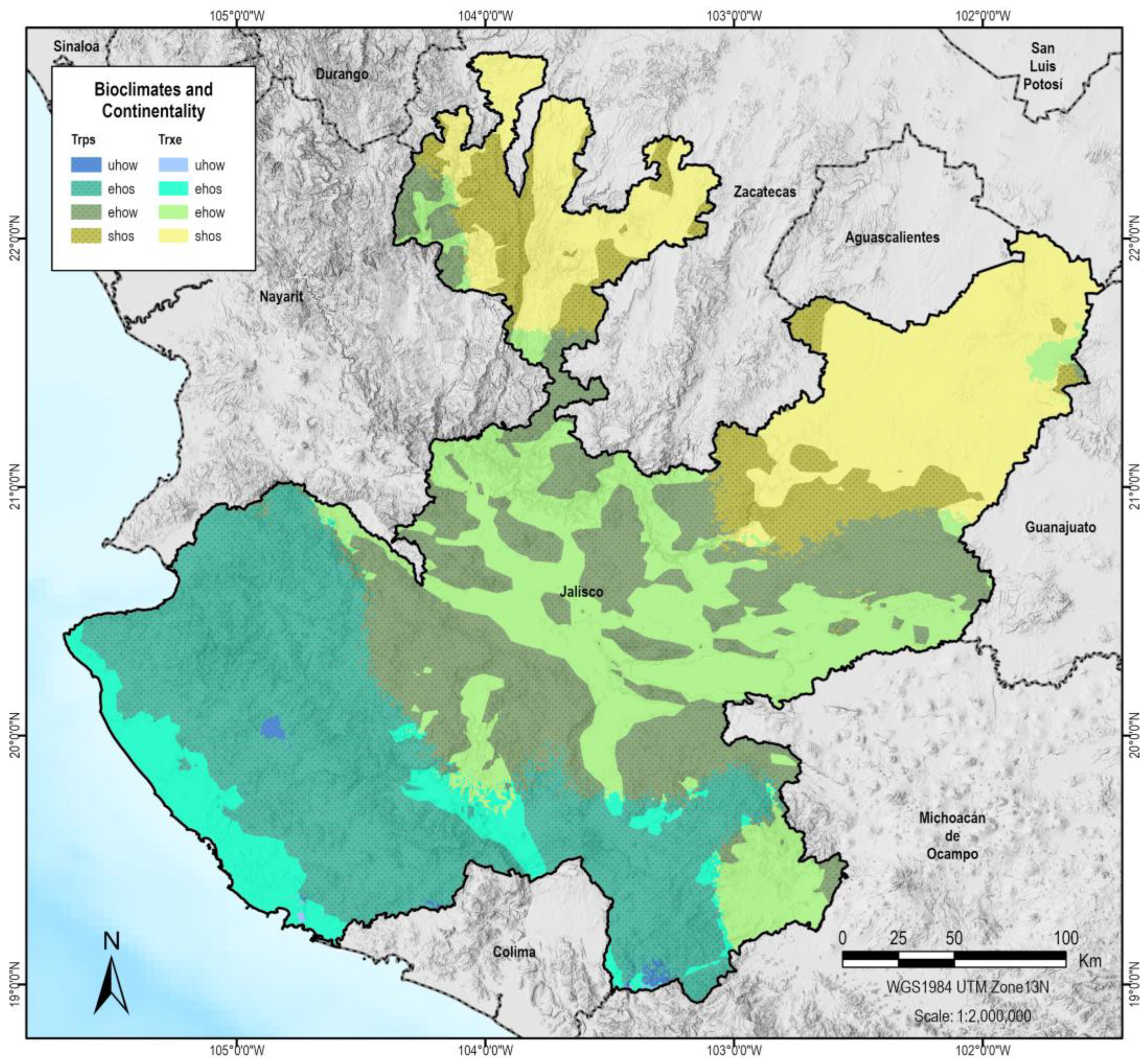
The study incorporates an analysis of continentality based on the continentality index, which expresses the average monthly thermal oscillation over the year in degrees Celsius. The degree of continentality is directly proportional to this amplitude, with its opposite being oceanity.

-

This research proposes a first approach of an alternative bioclimatic classification that enhances the understanding of the interrelationship between climate and the distribution of climatophyllous potential vegetation within the territory of Jalisco. This classification will be further developed in subsequent research.

2. Materials and Methods

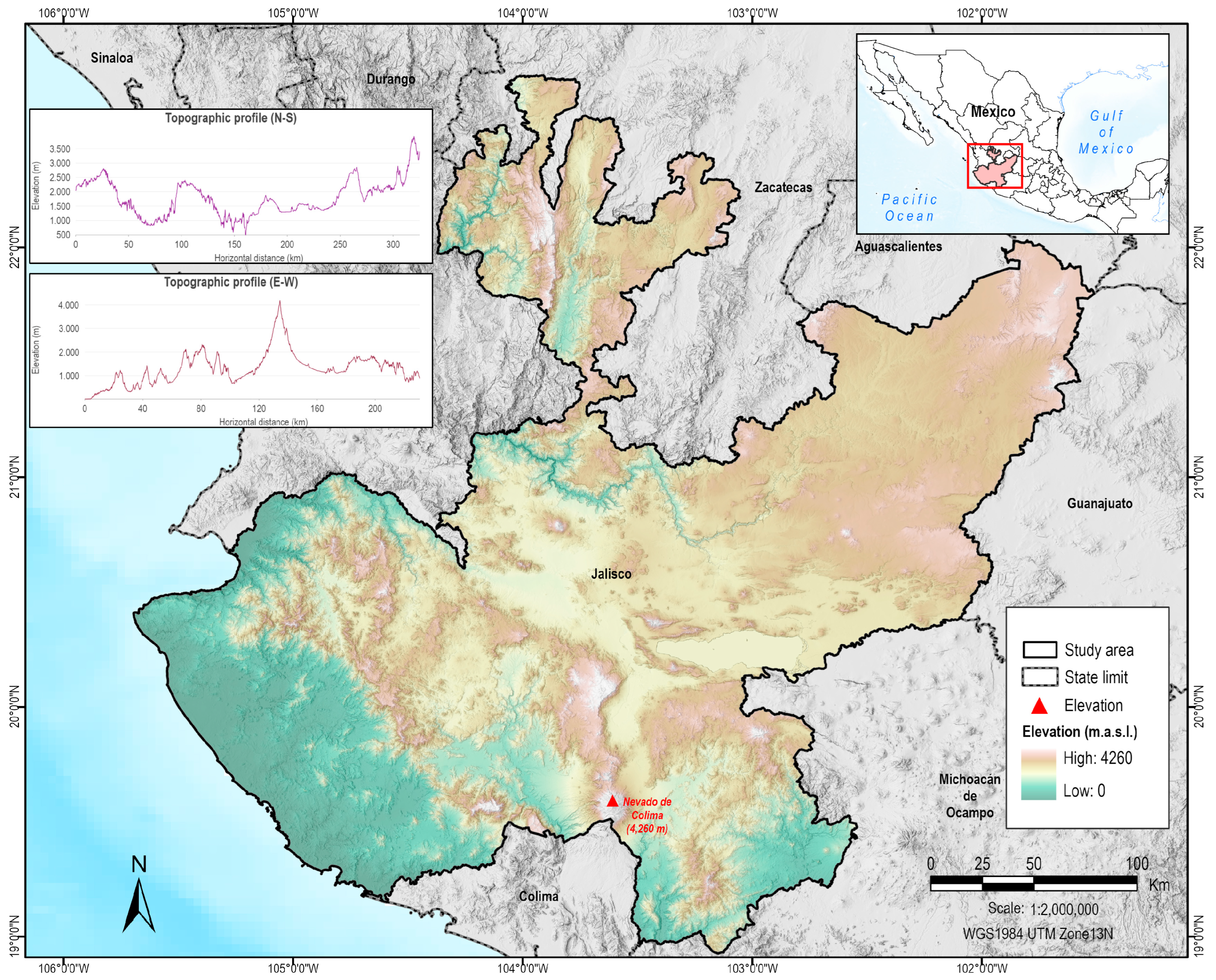
2.1. Study Area

The study area is located in the state of Jalisco, in the central-western region of Mexico (Figure 1). It spans extreme coordinates between 22°45′ and 18°55′ north latitude and 101°30′ and 105°41′ west longitude, covering approximately 78,590 km², which represents 4.0% of the national territory [41]. The elevation ranges from sea level to 4260 m asl at Nevado de Colima, the highest peak in the state. Jalisco is one of Mexico’s most geographically and ecologically representative regions due to its position at the convergence of six biogeographic provinces and its location within the Mexican Transition Zone. This transitional area integrates taxa of both Nearctic and Neotropical origins, resulting in high levels of topographic, climatic, bioclimatic, and phytocenotic diversity. The region’s complex geological history is marked by extensive volcanic activity, characterized by volcanic structures, lava flows, fractures, and normal faults. These features have shaped the landscape, forming extensive valleys and tectonic trenches, such as those associated with Lago de Chapala, the largest freshwater body in Mexico. Other significant water bodies in the state include Laguna de Atotonilco, Cajititlán, Sayula, San Marcos, and Zapotlán [42]. Geomorphologically, Jalisco exhibits a diverse range of landscapes, including the valleys of the Bolaños and Comatlán rivers, the Pajaritos and Alica volcanic mountain ranges, the Zacatecan mountain and valleys, and the acid block mountain range. Additional notable formations include the Colima Volcanic Complex, the Tapalpa block mountain region, and the Sierra del Tigre [43]. These features contribute to the region’s environmental complexity and its wide range of vegetation types. The dominant vegetation in Jalisco consists of coniferous forest, oak forest, and grasslands, largely influenced by the state’s temperate subhumid climate [44]. However, the region also supports diverse ecosystems such as subalpine scrublands, cloud forests (especially in ravines), and riparian vegetation. According to the INEGI [45,46], the state’s vegetation types include pine forests, juniper forests, oak forests, mountain cloud forests, subdeciduous forests, deciduous forests, thorny forests, crasicaule scrublands, and high mountain grasslands. Jalisco is also one of Mexico’s most floristically rich states, ranking fourth in the number of native plant species recorded. The state harbors 235 botanical families, 1541 genera, and 7155 species of vascular plants, of which 3353 are endemic to Mexico, and 182 are endemic to Jalisco [35]. The state exhibits a diverse range of climatic conditions, encompassing 29 distinct Köppen climatic variants [47]. The dry or semiarid climates BS₁ represent 13.78% of the state territory, while the warm humid Aw represents 21.77%, the semi-warm humid A(C)w 4.45%, the semi-warm humid (A)C(w) 41.67 %, the temperate humid Cw 18.33%, and the cold E 0.001%. From a bioclimatic perspective, Jalisco belongs to the Tropical macrobioclimate, which includes both Tropical pluviseasonal and Tropical xeric bioclimates [28,31].

Jalisco comprises six distinct biogeographic provinces: the Transmexican Volcanic Belt (TVB), the Sierra Madre del Sur (SMS), the Sierra Madre Occidental (SMO), the Pacific Lowlands (PL), the Chihuahuan Desert (CD), and the Balsas Basin (BB) [36]. The TVB province is in the central region of the country, at an altitude above 1800 m asl [48]. The geological history of this mountain system and its diverse biotic connections with other biogeographic provinces render it one of the most complex and heterogeneous provinces in the country [49]. The province exhibits a considerable degree of botanical diversity, with pine-oak forests representing the most prevalent vegetation type. However, tropical deciduous forests and xerophytic scrubland are also present [50,51]. In terms of the SMS, the province is characterized by elevations exceeding 1000 m asl and extends in a northwest-southeast direction parallel to the Pacific Ocean coastline. The region exhibits a remarkable climatic diversity. The predominant vegetation is that of temperate forests, particularly coniferous, pine-oak, and cloud forests [50,52,53]. The other province is the SMO, situated in the western region of the country, at elevations ranging from 200 to 3000 m asl. Most of its terrain is situated above 2000 m asl. It encompasses the longest and most continuous mountainous system within the country’s orographic systems. This system extends from the Pacific Ocean coast, situated to the south of the border with the United States, to the elevated regions of Nayarit and Jalisco, thus, connecting the Rocky Mountains with the TVB [53]. The predominant vegetation is pine and pine-oak forests [48,50,51,53]. The PL province is located along the Pacific coast of Mexico, occupying a narrow and uninterrupted strip of land. The elevation of the region is typically less than 400 m asl. The vegetation comprises seasonally dry tropical forests, humid tropical forests, and savannas [48,51,53]. This province is home to the highest concentration of seasonally dry tropical forests in the country [54]. Regarding the CD province, there exhibits a considerable range in altitude, spanning from 1000 to 2000 m asl. This province is situated within the Mexican Altiplano, which extends between the SMO and Sierra Madre Oriental. The province is characterized by the presence of numerous endorheic basins. The vegetation of this province comprises grass steppes belonging to the genera Bouteloua and Aristida, interspersed with xerophytic scrublands and forests in the plains and valleys [48,51,55]. The BB province is situated in central Mexico at an altitude below 2000 m asl. It corresponds to the Balsas River Basin, which is situated between TVB and the SMS. The vegetation comprises seasonally dry forests and grasslands [48,51,53].

2.2. Climate Database

Monthly average temperature and precipitation data for the state of Jalisco from 1980 to 2018 were obtained from the latest version (v2.1) of the CHELSA database (Climatologies at high resolution for the earth’s land surface areas) [56]. CHELSA provides high-resolution thermopluviometric data in raster format for any terrestrial region, with a spatial resolution of 30 arcseconds (0.88 km) [13]. The dataset was downscaled using temperature and precipitation estimates from the ERA-Interim climate reanalysis, ensuring a high-resolution representation of atmospheric conditions. ERA-Interim integrates model outputs with ground-based, radiosonde, and remote sensing observations through a data assimilation system, enhancing the accuracy of both free-atmosphere and surface fields [57]. The CHELSA temperature algorithm relies on statistical downscaling of atmospheric temperatures, while its precipitation algorithm incorporates orographic predictors such as wind fields, valley exposition, and boundary layer height, followed by a bias correction. To validate its results and bias correction steps, CHELSA applies statistical cross-validation, comparing outputs with other datasets of similar spatial and temporal resolution, as well as independent meteorological station data [13].

Additionally, a thorough and meticulous data validation process for our study area was rigorously implemented to provide a solid foundation for the investigation, with the aim of ensuring the reliability and validity of the data. This was achieved through the implementation of the Bland–Altman (B-A) method [58], which is based on quantifying the agreement between two quantitative measurements (observational data and high-resolution data) by examining the mean difference and constructing limits of agreement. The B-A method requires the calculation of the limits (d̅ − 2 sd, d̅ + 2 sd), where d̅ is the mean and sd is the standard deviation of the individual differences d = x − y. These limits are popularly known as Bland–Altman limits of agreement, although they are better understood as the limits of disagreement since they are based on differences. The value of d̅ is an estimate of the bias of one method over the other. Observations with differences outside the specified limits indicate discrepancies between the datasets at specific points. It is generally expected that the majority of data will fall within these limits, thus, providing a robust assessment of measurement agreement.

2.3. Bioclimatic Diagnosis

The bioclimatic characterization of the study area was conducted in accordance with the bioclimatic classification system proposed by Rivas-Martínez et al. [7]. The fundamental premise of this classification is the reciprocal and adjusted relationship between climate, vegetation, and geographical territories [59]. The macrobioclimate represents the highest level of typological organization within this bioclimatic system. It is an eclectic biophysical model, delimited by specific climatic and vegetational parameters, with a broad territorial jurisdiction and correlation with the predominant climatic types, biomes, and biogeographic regions on Earth. The subordinate unit of the macrobioclimate is the bioclimate, which serves as the fundamental unit of typological reference. Furthermore, variations in seasonal precipitation patterns (bioclimatic variants) and thermal or ombrothermal values (bioclimatic belts: thermotypes and ombrotypes) are observed within each bioclimate. The bioclimatic units are the distinct types of climatic conditions that occur in a latitudinal or altitudinal zonation. Each bioclimatic unit is characterized by specific plant formations and communities [7].

The following section describes the bioclimatic parameters and indices that have been employed for the delimitation and characterization of the bioclimatic units within the study area.

• Simple continentality index (Ic).

It is the numerical expression of the thermal amplitude of a given location, indicating the maximum range of average annual thermal oscillation. This index represents the discrepancy in temperature between the month with the highest average temperature of the year (Tmax) and the month with the lowest average temperature (Tmin).

Table 1. Types, subtypes, and levels of simple continentality (Ic) [7].

Types	Subtypes	Levels	Values (Ic)
Hyperoceanic	Ultrahyperoceanic	Ultrahyperoceanic strong	0.0–2.0
		Ultrahyperoceanic weak	2.0–4.0
	Euhyperoceanic	Euhyperoceanic strong	4.0–6.0
		Euhyperoceanic weak	6.0–8.0
	Subhyperoceanic	Subhyperoceanic strong	8.00–10.0
		Subhyperoceanic weak	10.0–11.0
Oceanic	Semihyperoceanic	Semihyperoceanic strong	11.0–12.0
		Semihyperoceanic weak	12.0–14.0
	Euoceanic	Euoceanic strong	14.0–15.0
		Euoceanic weak	15.0–17.0
	Semicontinental	Semicontinental weak	17.0–19.0
		Semicontinental strong	19.0–21.0
Continental	Subcontinental	Subcontinental weak	21.0–24.0
		Subcontinental strong	24.0–28.0
	Eucontinental	Eucontinental weak	28.0–37.0
		Eucontinental strong	37.0–46.0
	Hypercontinental	Hypercontinental weak	46.0–56.0
		Hypercontinental strong	56.0–66.0

illustrates the classification of continentality, as defined by the Ic, according to the types, subtypes, and levels of continentality. The mathematical formula for this index is as follows: Ic = Tmax − Tmin.

• Thermicity index (It).

This index is formulated using the average annual temperature (T), the average temperature of the maximums of the coldest monthly period (M), and the average temperature of the minimum of the coldest month (m). This index is also known as the cold index because it considers the intensity of the cold, which is a limiting factor for many plants and plant communities. This is a result of the fact that the winter period is the one that causes the greatest stress to the vegetation. The mathematical formula for this index is It = (T + M + m) * 10.

In extratropical territories, a modification of the It is made, recognizing the compensated thermicity index (Itc). This index considers the value of the It, due to the ‘excess’ of cold or warmth that occurs during the cold season in territories with a climate with a continental or highly hyperoceanic tendency. In this way, the continentality of these territories can be compared. In the case of an Ic falling between 8 and 18, the value of the Itc is equivalent to that of the It. Conversely, in the instance that the continentality index fails to reach or exceeds the values, the thermicity value must be compensated for by the addition or subtraction of a compensation value (Cἰ) (

Table 2. Calculation of compensation values (Cἰ) according to the value of the continentality index (Ic), to obtain the compensated thermicity index (Itc) [7].

Ic	fi	Ci	Max. Value
Ic ≤ 8	f0 = 10	Ci = C0; C0 = f0 (8 − Ic)	C0 = −80
18 < Ic ≤ 21	f1 = 5	Ci = C1; C1 = f1 (Ic − 18)	C1 = +15
21 < Ic ≤ 28	f2 = 15	Ci = C1 + C2; C1 = f1 (21 − 18) = 15; C2 = f2 (Ic − 21)	C2 = +105
28 < Ic ≤ 46	f3 = 25	Ci = C1 + C2 + C3; C1 = 15; C2 = f2 (28 − 21) = 105; C3 = f3 (Ic − 28)	C3 = +450
46 < Ic ≤ 65	f4 = 30	Ci = C1 + C2 + C3 + C4; C1 = 15; C2 = 105; C3 = f3 (46 − 28) = 450; C4 = f4 (Ic − 48)	C4 = +570

), as represented by the following formula: Itc = It ± Cἰ.

The Itc, or It, is employed to determine the thermotype, which represents the thermal component of the bioclimatic belt. The bioclimatic unit is determined based on the values of the It, if these are above the value of 120 and the Ic is less than 21. Otherwise, the values are determined through the positive temperature (Tp). A thermotypic altitudinal and latitudinal gradient is determined by the bioclimatic and vegetational characteristics. The determining values for the Tropical macrobioclimate are shown in

Table 3. Termoclimatic units of the Tropical macrobioclimate [59].

Thermotype	Abbr.	It, Itc	Tp: Ic ≥ 21, Itc < 120
Infratropical	itr	670–890	>2860
Thermotropical	ttr	490–670	>2300
Mesotropical	mtr	320–490	>1700
Supratropical	str	160–320	>1000
Orotropical	otr	< 160	500–1000
Cryorotropical	ctr	-	1–500
Gelid	gtr	-	0

.

• Annual ombrothermic index (Io).

This index demonstrates the correlation between positive precipitation (Pp) and positive temperature (Tp). Given that rainfall is always positive, this is not the case for temperatures. Consequently, those months in which average temperature values are below 0 °C are excluded from the calculation. In this situation, water resources are unavailable for vegetation. Therefore, it is the quotient between the sum of the average precipitation in millimeters of the months whose average temperature is greater than 0 °C and the sum of the average monthly temperature greater than 0 °C in tenths of a degree. Its mathematical formula is Io = (Pp/Tp) * 10.

The ombrotype represents the bioclimatic unit, delineated by the values of the Io, which defines the ombric component of the bioclimatic belt. In this instance, an altitudinal and latitudinal sequence is also evident within the bioclimatic units, characterized by ombrothermal values and the characteristics of the associated vegetation. The defining values of the identified ombrotypes for the Tropical macrobioclimate are presented in

Table 4. Ombroclimatic types of the Tropical macrobioclimate [59].

Ombroclimatic Type	Abbr.	Io
UItrahyperarid	uha	<0.2
Hyperarid	har	0.2–0.4
Arid	ari	0.4–1.0
Semiarid	sar	1.0–2.0
Dry	dry	2.0–3.6
Subhumid	shu	3.6–6.0
Humid	hum	6.0–12.0
Hyperhumid	hhu	12.0–24.0
Ultrahyperhumid	uhh	24.0–48.0
Extreme hyperhumid	ehh	>48.0

.

Furthermore, in the Tropical macrobioclimate, the ombrothermic index of the driest two months in the driest quarter of the year (Iod₂) is crucial for identifying the bioclimate, the fundamental unit of this bioclimatic classification system. The values of each bioclimate within the Tropical macrobioclimate are presented in

Table 5. Bioclimatic ranges and bioclimates of the Tropical macrobioclimate [7].

Bioclimate	Abbr.	Io	Iod2
Tropical pluvial	Trpl	≥3.6	>2.5
Tropical pluviseasonal	Trps	≥3.6	≤2.5
Tropical xeric	Trxe	1.0–3.6	-
Tropical desertic	Trde	0.2–1.0	-
Tropical hyperdesertic	Trhd	<0.2	-

.

The bioclimatic variants are units of typological bioclimatology that are recognized within specific bioclimates, and which make it possible to identify climatic peculiarities of an ombric and occasionally thermic nature. The bioclimatic variables are steppic, submediterranean, bixeric, antitropical, tropical drought, seropluvial, polar semiboreal, and semitropical hyperdesertic [7].

Table 6. Distribution of bioclimatic variables in the macriobioclimates of the Earth. Tr = Tropical, Me = Mediterranean, Te = Temperate, Bo = Boreal, Po = Polar, * means presence and—absence [7].

Bioclimate Variable	Tr	Me	Te	Bo	Po
Submediterranean	-	-	*	*	*
Steppic	-	*	*	*	*
Bixeric	*	-	-	-	-
Antitropical	*	-	-	-	-
Seropluvial	*	-	-	-	-
Tropical drought	*	-	-	-	-
Polar semiboreal	-	-	-	*	*
Semitropical hyperdesertic	*	*	-	-	-

shows the distribution of bioclimatic variables that are recognized in the macrobioclimates of the Earth.

In the context of the basic isobioclimate, the term refers to a model that is formed by combining principally three key elements: bioclimate, thermotype, and ombrotype. Each isobioclimate is characterized by a distinct bioclimate space, which can be delineated by the threshold values of the individual bioclimatic units that comprise it. Furthermore, to nuance the isobioclimates, the meroisobioclimate is recognized as a lower-ranking bioclimatic typological unit than the isobioclimate, which is delineated by the continentality values [7]. The bioclimatic models or spaces are useful for identifying similar territories and equivalent types of vegetation, as well as for creating highly precise bioclimatic maps. In this study, the isobioclimates were employed as the bioclimatic unit to establish a correlation between them and the climatophyllous potential vegetation types present in the study area.

2.4. Bioclimatic Cartography

The required calculations were performed using the thermopluviometric data in raster format obtained from the CHELSA v2.1 database [56], which enabled the determination of values of the specified bioclimatic indices and parameters. The CHELSA v2.1 dataset provides high-resolution (30 arc-seconds) interpolated climatic variables, incorporating statistical downscaling, machine learning, and orographic correction techniques. Given that this dataset already integrates advanced interpolation methods, no additional geostatistical techniques, such as kriging, were applied in this study. The results were represented as six maps illustrating bioclimates, continentality, bioclimatic variants, thermotypes, ombrotypes, and isobioclimates. This was achieved by utilizing the WGS 1984 geographic coordinate system and the UTM Zone 13N projection. The calculations were performed using map algebra in ArcGIS Pro v3.2.2 [60], specifically through the Raster Calculator tool. This tool allows for the creation and execution of map algebra expressions to generate raster outputs, leveraging the full range of Spatial Analyst functions, tools, and operators for geographic analysis. Subsequently, to refine spatial representation, edge smoothing and error correction techniques were applied, ensuring consistency and accuracy in the final outputs.

2.5. Diagnosis of Potential Vegetation and Its Correspondence with Bioclimatic Units

The interaction between flora, soil, and climate gives rise to patterns of plant communities, or biomes, within which different types of vegetation can be identified [53]. In Mexico, numerous contributions have been made to the characterization and classification of vegetation types. These include works by Miranda and Hernández-X [61], Rzedowski [50], Pennington and Sarukhán [62], González-Medrano [63], and Challenger and Soberón [64]. Based on the primary categories of vegetation outlined in these proposals, Villaseñor and Ortiz [65] synthesized five principal biomes for the country: seasonally dry tropical forest, humid mountain forest, temperate forest, humid tropical forest, and xerophilous scrublands. These biomes were subsequently organized into distinct vegetation types. However, in INEGI [46] they adapted the proposals of Miranda and Hernández-X [61], Flores-Mata et al. [66], and Rzedowski [50] to the cartographic criteria and represented them in the land use and vegetation layer series VII scale 1:250,000. The system is organized such that classes are grouped according to the characteristics of the different types of vegetation; this allows for the definition of large groups of vegetation with ecological and physiognomic affinity in the first order. Accordingly, this layer comprises 182 classes and includes a dictionary that elucidates the spectral attributes of each class, as well as the most prevalent genera and species found within each class [45,46].

Once the bioclimatic characterization of the study area was obtained and the corresponding cartography was prepared, the correspondence between the isobioclimates and potential vegetation was analyzed in accordance with the climatophyllous vegetation types that had been identified in the study area based on the information contained in INEGI [45,46]. The term ‘climatophyllous’ is used to describe plant communities that are linked to and determined by climate. These communities develop in habitats where mature or zonal soils receive only rainwater according to the ombrotype of the territory. In this context, the climatophyllous potential vegetation types proposed for the study area have been selected in accordance with the criteria established by Giménez and González [67], Giménez et al. [30], Macías-Rodríguez et al. [8,22], and Gopar-Merino et al. [9,23].

Subsequently, the spatial join tool in ArcGIS Pro v3.2.2 was employed [60]. The isobioclimate layer and the adjusted land use and vegetation layer were then superimposed, resulting in the generation of a new layer from which the isobioclimate information and its corresponding climatophyllous potential vegetation type were subsequently extracted. The resulting model data were expressed in shapefile format layers for subsequent analysis. Additionally, a comprehensive review of the data were conducted, and any inconsistencies in the classification of vegetation types in relation to the expected isobioclimate were accounted for to ensure accuracy and precision.

3. Results

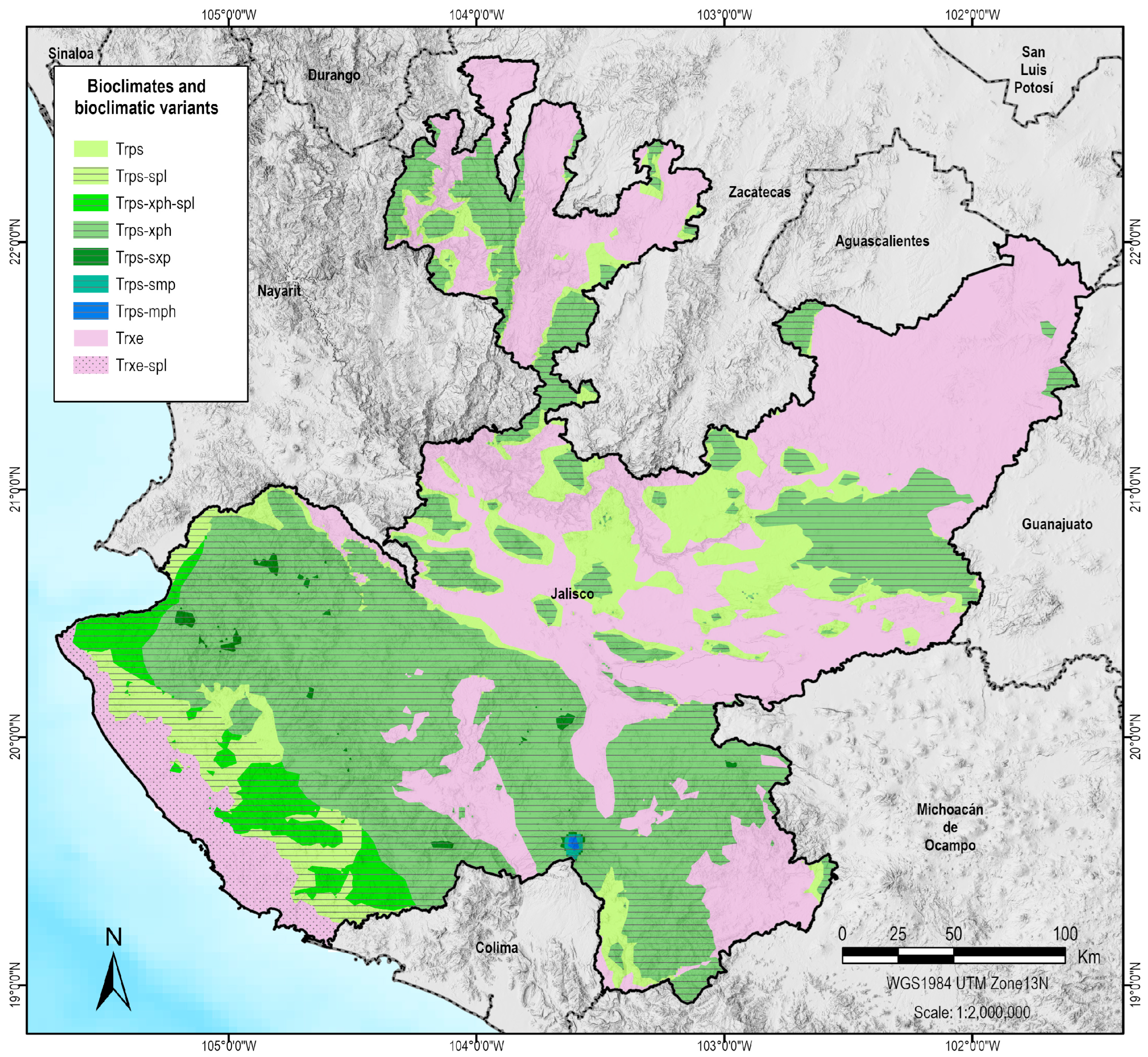
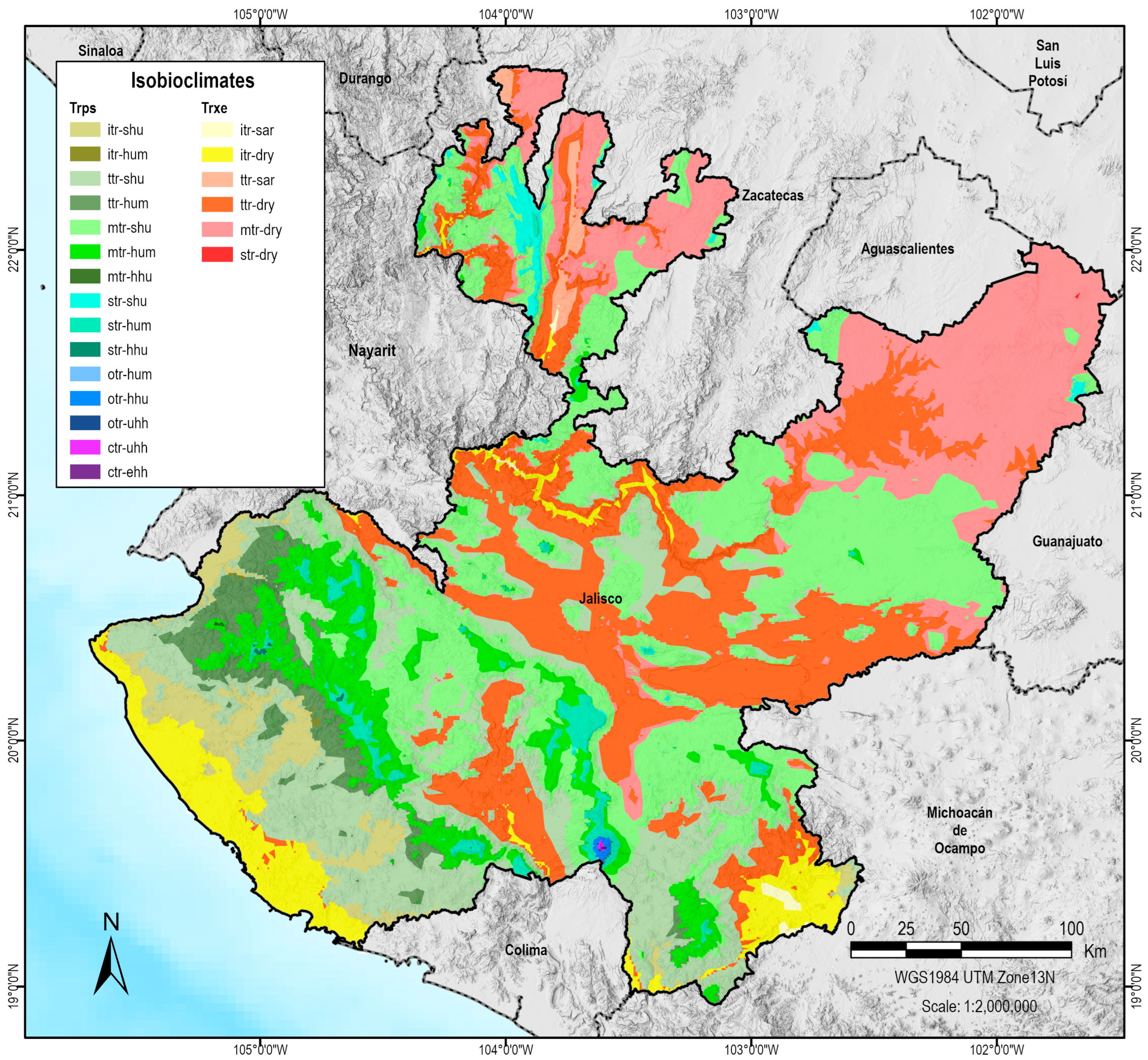
3.1. Bioclimatic Characterization

The bioclimatic diagnosis was conducted to identify the bioclimatic units present in the state of Jalisco. The territory is recognized as belonging to the tropical macrobioclimate. In addition to its geographical situation, the amount of annual rainfall, seasonal rainfall, and annual rhythm of rainfall determine the presence of two of the five global bioclimates: Tropical pluviseasonal (Trps) and Tropical xeric (Trxe). The Trps bioclimate is present in 56.62% of the area, while the Trxe bioclimate is in 43.38%. Figure 2 illustrates their spatial distribution in the study area.

The seasonal rhythm of rainfall and the daily and seasonal rhythms of temperature throughout the year play an integral role in the composition and distribution of plant communities. These factors hold as much or more importance as the amount of rainfall and the annual and monthly average temperature. Such variations in rainfall and temperature patterns serve as key determinants of both bioclimatic units and the bioclimatic variants. The region is distinguished by two distinct bioclimatic variants: seropluvial and tropical drought. It is noteworthy that 49.84% of the territory exhibits the presence of the bioclimatic variants. The seropluvial (spl) bioclimatic variant is characterized by a reduction in rainfall during the first months of the summer solstice, with precipitation levels being at least 1.3 times lower than the average rainfall recorded in the subsequent two months. This bioclimatic variant indicates monsoonal bioclimates, which in this study are identified in Trps and Trxe bioclimates. These are characterized by the arrival of rain in the late summer months due to the monzonic flow, which is generated by the thermal contrast between a continental mass of air and the Pacific Ocean. This phenomenon develops in a manner analogous to that of breezes. This can correspond to the transition zones between the Aw (warm sub-humid with summer rainfall) and the BSw (semi-dry or steppe with summer rainfall), according to the Köppen–Geiger classification system [68], as evidenced in Chamela-Cuixmala, where the early summer drought is compensated by subsequent rainfall. In contrast, the tropical drought is manifested exclusively in the Trps bioclimate, in territories with a subhumid to extreme hyperhumid ombrotype, wherein drought is defined as occurring in months with an ombrothermic index below 2.5. The monthly tropical drought value is calculated by subtracting 250 from the amount of the monthly ombrothermic index in tenths of a degree. The tropical drought ombrovariables are established in accordance with the tropical drought indices, which are defined as the sum of the monthly tropical drought values over the course of a year. There are seven tropical drought ombrovariables, but only four of them are expressed in the area, with values ranging from 1 to >1700 of the tropical drought indices. These are categorized as pluviseasonal mesophytic (mph), pluviseasonal submesophytic (smp), pluviseasonal subxerophytic (sxp), and pluviseasonal xerophytic (xph). Figure 3 provides a visual representation of the spatial distribution of these bioclimatic variants.

The index that is utilized to delineate the bioclimate is the simple continentality index or the annual thermic interval. The range or amplitude between these temperatures, expressed in degrees Celsius, has a significant impact on the distribution of vegetation and, consequently, on the boundaries of many bioclimates [69]. In this analysis, the most oceanic level of simple continentality identified for both bioclimates is specifically the ultrahyperoceanic weak (uhow: 0.28%), followed by the euhyperoceanic strong (ehos: 33.35%), euhyperoceanic weak (ehow: 41.24%), and the least oceanic, and the subhyperoceanic strong (shos: 25.11%). Figure 4 shows their spatial distribution in the study area.

The bioclimatic belts are each of the spaces and types of climatic conditions that occur in an altitudinal or latitudinal clinosequence. The delimitation of these belts is based on the thermoclimatic indices (It, Itc, Tp) and the annual ombrothermic index (Io). Each bioclimatic belt is distinguished by a particular composition of plant formations and communities [7]. Thermotypes are defined as bioclimatic units that are associated with a specific macrobioclimate. In the study area, the following thermoclimatic ranges were identified: infratropical (itr: 9.95%), thermotropical (ttr: 41.48%), mesotropical (mtr: 45.90%), supratropical (str: 2.58%), orotropical (otr: 0.08%), and cryorotropical (ctr: 0.01%). The spatial representation in the study area of these bioclimatic units is illustrated in Figure 5, which highlights the thermicity in the plain areas, the canyons, and the valley bottoms. As the positive temperature increases, the thermotypes are more thermic. This phenomenon has been observed in locations with lower elevations. In contrast, in mountainous regions, there is a decrease in positive temperature with increasing altitude. The itr thermotype is predominantly located along the Pacific coastline, though it is also found in the canyons of the Grande de Santiago River and the valley bottoms of the Balsas Basin. The most representative thermotypes in the area are thermotropical and mesotropical, which together represent almost 90% of the total. The ttr thermotype is found in valleys and some mountains between 200 and 2000 m asl, while the mtr thermotype is in higher mountains (1000–2800 m asl) and areas where there is less thermicity. The str thermotype is established at higher elevations (2000–2800 m asl) in more restricted areas. The otr thermotype is observed from an elevation of >2800 m asl, while the ctr thermotype is identified from an elevation of >3450 m asl. The two latest thermotypes are recognized at the highest elevations, as evidenced by their presence at the Nevado de Colima, which reaches an elevation of 4260 m asl. This mountain is the highest elevation in the territory analyzed.

The ombrotypes present in the territory comprise semiarid (sar: 0.89%), dry (dry: 42.49%), subhumid (shu: 44.58%), humid (hum: 11.92%), hyperhumid (hhu: 0.10%), ultrahyperhumid (uhh: 0.01%), and extreme hyperhumid (ehh: 0.001%). The sar ombrotype is represented in the small patches to the north, bordering the states of Zacatecas and Durango along the Atengo River and the canyons of the SMO province, as well as in the canyons of the Bolaños River and the Chico River in the north of the Jalisco state. However, this ombrotype is present in a limited area in the southern portion of the study region, specifically in the BB province, adjacent to the state of Michoacán, along the canyons of the Tepalcatepec River and in the northwest portion of the Presa Constitución of Apatzingán. The dry ombrotype is the second most widely distributed in the study area, developing in almost all coastal territories belonging to the PL province, as well as in the plateaus belonging to the provinces of SMO, CD, and part of the TVB, and the entire portion corresponding to the BB province. The shu ombrotype is the most representative in the territory. It is present in the mountain regions corresponding principally to the provinces of SMO, TVB, and SMS. Moreover, it also exists in the east of the state in the mountains of CD province. The hum and hhu ombrotypes are observed in limited areas situated in elevated locations, typically within canyons and their associated slopes. The most humid ombroclimatic types correspond to the uhh and ehh ombrotypes, with a maximum value of Io equal to 30.44 and 51.70, respectively. These are only localized in the Nevado de Colima. In contrast, the areas with the driest ombroclimatic type agree with the sar ombrotype, with a minimum value of Io equal to 1.78 in the north of the state of Jalisco, bordering the states of Durango and Zacatecas, and in some areas in the south of the state in the BB province. A map illustrating the distribution of each ombrotype is provided in Figure 6.

In order to identify the basic isobioclimates present in the study area, a combined analysis was conducted among two bioclimates, six thermotypes, and seven ombrotypes. The investigation has identified 21 basic isobioclimates (

Table A1. Basic isobioclimates identified in the state of Jalisco. Acronyms: Trps = Tropical pluviseasonal; Trxe = Tropical xeric; itr = infratropical; ttr = thermotropical; mtr = mesotropical; str = supratropical; otr = orotropical; ctr = cryorotropical; sar = semiarid; dry = dry; shu = subhumid; hum = humid; hhu = hyperhumid; uhh = ultrahyperhumid; ehh = extreme hyperhumid.

No.	Bioclimate	Thermotype	Ombrotype	Isobioclimate
1	Trps	ctr	ehh	Trps-ctr-ehh
2	Trps	ctr	uhh	Trps-ctr-uhh
3	Trps	otr	uhh	Trps-otr-uhh
4	Trps	otr	hhu	Trps-otr-hhu
5	Trps	otr	hum	Trps-otr-hum
6	Trps	str	hhu	Trps-str-hhu
7	Trps	str	hum	Trps-str-hum
8	Trps	str	shu	Trps-str-shu
9	Trps	mtr	hhu	Trps-mtr-hhu
10	Trps	mtr	hum	Trps-mtr-hum
11	Trps	mtr	shu	Trps-mtr-shu
12	Trps	ttr	hum	Trps-ttr-hum
13	Trps	ttr	shu	Trps-ttr-shu
14	Trps	itr	hum	Trps-itr-hum
15	Trps	itr	shu	Trps-itr-shu
16	Trxe	str	dry	Trxe-str-dry
17	Trxe	mtr	dry	Trxe-mtr-dry
18	Trxe	ttr	dry	Trxe-ttr-dry
19	Trxe	ttr	sar	Trxe-ttr-sar
20	Trxe	itr	dry	Trxe-itr-dry
21	Trxe	itr	sar	Trxe-itr-sar

), and their distribution in the territory can be observed in Figure 7. The most representative basic isobioclimates in the territory correspond to the Tropical pluviseasonal mesotropical subhumid (Trps-mtr-shu), Tropical xeric thermotropical dry (Trxe-ttr-dry), Tropical pluviseasonal thermotropical subhumid (Trps-ttr-shu), Tropical xeric mesotropical dry (Trxe-mtr-dry), Tropical pluviseasonal mesotropical humid (Trps-mtr-hum), Tropical xeric infratropical dry (Trxe-itr-dry), Tropical pluviseasonal infratropical subhumid (Trps-itr-shu), Tropical pluviseasonal thermotropical humid (Trps-ttr-hum), and Tropical pluviseasonal supratropical humid (Trps-str-hum). These nine isobioclimates collectively represent 98.19% of the study area, whereas the remaining twelve isobioclimates account for a minor proportion of just 1.81%.

However, in accordance with the bioclimatic system, these units were nuanced with the two identified bioclimatic variants present in the study area. This resulted in the identification of 42 distinct isobioclimates. In 32 of these isobioclimates, at least one bioclimatic variant was identified, while in 10, no such bioclimatic variant was present. A correlation was, thus, established between the distribution of climatophyllous potential vegetation, and the results are presented in Figure 8. To provide further nuance, the continentality values were included to delineate a lower-ranking bioclimatic typological unit than isobioclimate, resulting in the recognition of the meroisobioclimate. Furthermore, the thermotypic horizons, representing the upper or lower half of the thermic interval of the thermotype, and the ombric horizons, which indicate the threshold values based on the rainfall and rising evaporation as the temperature increases, were also considered. This encompasses 162 distinct meroisobioclimates within the study area. It should be noted that this level of detail is not represented on a map in this research due to the size and the complexity of these bioclimatic units, but the results are presented in the Appendix A as a table (

Table A2. Meroisobioclimates identified in the state of Jalisco. Acronyms: Trps = Tropical pluviseasonal; Trxe = Tropical xeric; uhow = ultrahyperoceanic weak; ehos = euhyperoceanic strong; ehow = euhyperoceanic weak; shos = subhyperoceanic strong; spl = seropluvial; xph = xerophytic; sxp = subxerophytic; smp = submesophytic; mph = mesophytic; low = lower; upp = upper; itr = infratropical; ttr = thermotropical; mtr = mesotropical; str = supratropical; otr = orotropical; ctr = cryorotropical; sar = semiarid; dry = dry; shu = subhumid; hum = humid; hhu = hyperhumid; uhh = ultrahyperhumid; ehh = extreme hyperhumid.

No.	Bioclimate	Continentality	Bioclimatic Variant	Thermotypic Horizon		Ombric Horizon		Meroisobioclimate
1	Trps	ehos	mph	low	ctr	ehh		Trps-ehos-mph-low-ctr-ehh
2	Trps	ehos	mph	low	ctr	upp	uhh	Trps-ehos-mph-low-ctr-upp-uhh
3	Trps	ehos	mph	low	ctr	low	uhh	Trps-ehos-mph-low-ctr-low-uhh
4	Trps	ehos	mph	upp	otr	low	uhh	Trps-ehos-mph-upp-otr-low-uhh
5	Trps	ehos	mph	upp	otr	upp	hhu	Trps-ehos-mph-upp-otr-upp-hhu
6	Trps	ehos	smp	upp	otr	upp	hhu	Trps-ehos-smp-upp-otr-upp-hhu
7	Trps	ehos	smp	upp	otr	low	hhu	Trps-ehos-smp-upp-otr-low-hhu
8	Trps	ehos	smp	low	otr	low	hhu	Trps-ehos-smp-low-otr-low-hhu
9	Trps	ehos	sxp	low	otr	low	hhu	Trps-ehos-sxp-low-otr-low-hhu
10	Trps	ehos	smp	low	otr	upp	hum	Trps-ehos-smp-low-otr-upp-hum
11	Trps	ehos	smp	upp	str	low	hhu	Trps-ehos-smp-upp-str-low-hhu
12	Trps	ehos	sxp	upp	str	low	hhu	Trps-ehos-sxp-upp-str-low-hhu
13	Trps	ehos	smp	upp	str	upp	hum	Trps-ehos-smp-upp-str-upp-hum
14	Trps	ehos	sxp	upp	str	upp	hum	Trps-ehos-sxp-upp-str-upp-hum
15	Trps	ehos	xph	upp	str	upp	hum	Trps-ehos-xph-upp-str-upp-hum
16	Trps	ehos	sxp	upp	str	low	hum	Trps-ehos-sxp-upp-str-low-hum
17	Trps	ehos	xph	upp	str	low	hum	Trps-ehos-xph-upp-str-low-hum
18	Trps	ehow	sxp	upp	str	low	hum	Trps-ehow-sxp-upp-str-low-hum
19	Trps	ehow	xph	upp	str	low	hum	Trps-ehow-xph-upp-str-low-hum
20	Trps	shos	xph	upp	str	low	hum	Trps-shos-xph-upp-str-low-hum
21	Trps	ehos	sxp	low	str	low	hhu	Trps-ehos-sxp-low-str-low-hhu
22	Trps	ehos	xph	low	str	low	hhu	Trps-ehos-xph-low-str-low-hhu
23	Trps	ehos	sxp	low	str	upp	hum	Trps-ehos-sxp-low-str-upp-hum
24	Trps	ehos	xph	low	str	upp	hum	Trps-ehos-xph-low-str-upp-hum
25	Trps	ehos	sxp	low	str	low	hum	Trps-ehos-sxp-low-str-low-hum
26	Trps	ehos	xph	low	str	low	hum	Trps-ehos-xph-low-str-low-hum
27	Trps	ehow	sxp	low	str	low	hum	Trps-ehow-sxp-low-str-low-hum
28	Trps	ehow	xph	low	str	low	hum	Trps-ehow-xph-low-str-low-hum
29	Trps	shos	xph	low	str	low	hum	Trps-shos-xph-low-str-low-hum
30	Trps	ehow	xph	low	str	upp	shu	Trps-ehow-xph-low-str-upp-shu
31	Trps	shos	xph	low	str	upp	shu	Trps-shos-xph-low-str-upp-shu
32	Trps	shos	absence	low	str	low	shu	Trps-shos-low-str-low-shu
33	Trps	shos	xph	low	str	low	shu	Trps-shos-xph-low-str-low-shu
34	Trps	ehos	sxp	upp	mtr	low	hhu	Trps-ehos-sxp-upp-mtr-low-hhu
35	Trps	ehos	sxp	upp	mtr	upp	hum	Trps-ehos-sxp-upp-mtr-upp-hum
36	Trps	ehos	xph	upp	mtr	upp	hum	Trps-ehos-xph-upp-mtr-upp-hum
37	Trps	ehos	xph	upp	mtr	low	hum	Trps-ehos-xph-upp-mtr-low-hum
38	Trps	ehow	xph	upp	mtr	low	hum	Trps-ehow-xph-upp-mtr-low-hum
39	Trps	shos	xph	upp	mtr	low	hum	Trps-shos-xph-upp-mtr-low-hum
40	Trps	ehos	xph	upp	mtr	upp	shu	Trps-ehos-xph-upp-mtr-upp-shu
41	Trps	ehow	xph	upp	mtr	upp	shu	Trps-ehow-xph-upp-mtr-upp-shu
42	Trps	shos	xph	upp	mtr	upp	shu	Trps-shos-xph-upp-mtr-upp-shu
43	Trps	ehos	xph	upp	mtr	low	shu	Trps-ehos-xph-upp-mtr-low-shu
44	Trps	ehow	absence	upp	mtr	low	shu	Trps-ehow-upp-mtr-low-shu
45	Trps	ehow	xph	upp	mtr	low	shu	Trps-ehow-xph-upp-mtr-low-shu
46	Trps	shos	absence	upp	mtr	low	shu	Trps-shos-upp-mtr-low-shu
47	Trps	shos	xph	upp	mtr	low	shu	Trps-shos-xph-upp-mtr-low-shu
48	Trps	ehos	sxp	low	mtr	low	hhu	Trps-ehos-sxp-low-mtr-low-hhu
49	Trps	ehos	sxp	low	mtr	upp	hum	Trps-ehos-sxp-low-mtr-upp-hum
50	Trps	ehos	xph	low	mtr	upp	hum	Trps-ehos-xph-low-mtr-upp-hum
51	Trps	uhow	xph	low	mtr	low	hum	Trps-uhow-xph-low-mtr-low-hum
52	Trps	ehos	xph	low	mtr	low	hum	Trps-ehos-xph-low-mtr-low-hum
53	Trps	ehow	xph-spl	low	mtr	low	hum	Trps-ehow-xph-spl-low-mtr-low-hum
54	Trps	ehow	xph	low	mtr	low	hum	Trps-ehow-xph-low-mtr-low-hum
55	Trps	uhow	xph	low	mtr	upp	shu	Trps-uhow-xph-low-mtr-upp-shu
56	Trps	ehos	xph	low	mtr	upp	shu	Trps-ehos-xph-low-mtr-upp-shu
57	Trps	ehow	xph-spl	low	mtr	upp	shu	Trps-ehow-xph-spl-low-mtr-upp-shu
58	Trps	ehow	absence	low	mtr	upp	shu	Trps-ehow-low-mtr-upp-shu
59	Trps	ehow	xph	low	mtr	upp	shu	Trps-ehow-xph-low-mtr-upp-shu
60	Trps	shos	xph	low	mtr	upp	shu	Trps-shos-xph-low-mtr-upp-shu
61	Trps	ehos	xph	low	mtr	low	shu	Trps-ehos-xph-low-mtr-low-shu
62	Trps	ehow	absence	low	mtr	low	shu	Trps-ehow-low-mtr-low-shu
63	Trps	ehow	xph	low	mtr	low	shu	Trps-ehow-xph-low-mtr-low-shu
64	Trps	shos	absence	low	mtr	low	shu	Trps-shos-low-mtr-low-shu
65	Trps	shos	xph	low	mtr	low	shu	Trps-shos-xph-low-mtr-low-shu
66	Trps	ehos	sxp	upp	ttr	upp	hum	Trps-ehos-sxp-upp-ttr-upp-hum
67	Trps	ehos	xph	upp	ttr	upp	hum	Trps-ehos-xph-upp-ttr-upp-hum
68	Trps	ehos	xph	upp	ttr	low	hum	Trps-ehos-xph-upp-ttr-low-hum
69	Trps	ehow	xph-spl	upp	ttr	low	hum	Trps-ehow-xph-spl-upp-ttr-low-hum
70	Trps	ehow	xph	upp	ttr	low	hum	Trps-ehow-xph-upp-ttr-low-hum
71	Trps	uhow	xph	upp	ttr	upp	shu	Trps-uhow-xph-upp-ttr-upp-shu
72	Trps	ehos	absence	upp	ttr	upp	shu	Trps-ehos-upp-ttr-upp-shu
73	Trps	ehos	xph	upp	ttr	upp	shu	Trps-ehos-xph-upp-ttr-upp-shu
74	Trps	ehow	xph-spl	upp	ttr	upp	shu	Trps-ehow-xph-spl-upp-ttr-upp-shu
75	Trps	ehow	absence	upp	ttr	upp	shu	Trps-ehow-upp-ttr-upp-shu
76	Trps	ehow	xph	upp	ttr	upp	shu	Trps-ehow-xph-upp-ttr-upp-shu
77	Trps	uhow	absence	upp	ttr	low	shu	Trps-uhow-upp-ttr-low-shu
78	Trps	uhow	xph	upp	ttr	low	shu	Trps-uhow-xph-upp-ttr-low-shu
79	Trps	ehos	absence	upp	ttr	low	shu	Trps-ehos-upp-ttr-low-shu
80	Trps	ehos	xph	upp	ttr	low	shu	Trps-ehos-xph-upp-ttr-low-shu
81	Trps	ehow	xph-spl	upp	ttr	low	shu	Trps-ehow-xph-spl-upp-ttr-low-shu
82	Trps	ehow	absence	upp	ttr	low	shu	Trps-ehow-upp-ttr-low-shu
83	Trps	ehow	xph	upp	ttr	low	shu	Trps-ehow-xph-upp-ttr-low-shu
84	Trps	shos	absence	upp	ttr	low	shu	Trps-shos-upp-ttr-low-shu
85	Trps	shos	xph	upp	ttr	low	shu	Trps-shos-xph-upp-ttr-low-shu
86	Trps	ehos	xph	low	ttr	low	hum	Trps-ehos-xph-low-ttr-low-hum
87	Trps	ehow	xph-spl	low	ttr	low	hum	Trps-ehow-xph-spl-low-ttr-low-hum
88	Trps	ehow	xph	low	ttr	low	hum	Trps-ehow-xph-low-ttr-low-hum
89	Trps	uhow	xph	low	ttr	upp	shu	Trps-uhow-xph-low-ttr-upp-shu
90	Trps	ehos	absence	low	ttr	upp	shu	Trps-ehos-low-ttr-upp-shu
91	Trps	ehos	spl	low	ttr	upp	shu	Trps-ehos-spl-low-ttr-upp-shu
92	Trps	ehos	xph	low	ttr	upp	shu	Trps-ehos-xph-low-ttr-upp-shu
93	Trps	ehow	xph-spl	low	ttr	upp	shu	Trps-ehow-xph-spl-low-ttr-upp-shu
94	Trps	ehow	xph	low	ttr	upp	shu	Trps-ehow-xph-low-ttr-upp-shu
95	Trps	uhow	absence	low	ttr	low	shu	Trps-uhow-low-ttr-low-shu
96	Trps	uhow	spl	low	ttr	low	shu	Trps-uhow-spl-low-ttr-low-shu
97	Trps	uhow	xph	low	ttr	low	shu	Trps-uhow-xph-low-ttr-low-shu
98	Trps	ehos	xph-spl	low	ttr	low	shu	Trps-ehos-xph-spl-low-ttr-low-shu
99	Trps	ehos	absence	low	ttr	low	shu	Trps-ehos-low-ttr-low-shu
100	Trps	ehos	spl	low	ttr	low	shu	Trps-ehos-spl-low-ttr-low-shu
101	Trps	ehos	xph	low	ttr	low	shu	Trps-ehos-xph-low-ttr-low-shu
102	Trps	ehow	xph-spl	low	ttr	low	shu	Trps-ehow-xph-spl-low-ttr-low-shu
103	Trps	ehow	absence	low	ttr	low	shu	Trps-ehow-low-ttr-low-shu
104	Trps	ehow	xph	low	ttr	low	shu	Trps-ehow-xph-low-ttr-low-shu
105	Trps	ehos	xph	upp	itr	low	hum	Trps-ehos-xph-upp-itr-low-hum
106	Trps	uhow	absence	upp	itr	upp	shu	Trps-uhow-upp-itr-upp-shu
107	Trps	uhow	xph	upp	itr	upp	shu	Trps-uhow-xph-upp-itr-upp-shu
108	Trps	ehos	absence	upp	itr	upp	shu	Trps-ehos-upp-itr-upp-shu
109	Trps	ehos	spl	upp	itr	upp	shu	Trps-ehos-spl-upp-itr-upp-shu
110	Trps	ehos	xph	upp	itr	upp	shu	Trps-ehos-xph-upp-itr-upp-shu
111	Trps	ehow	xph-spl	upp	itr	upp	shu	Trps-ehow-xph-spl-upp-itr-upp-shu
112	Trps	ehow	xph	upp	itr	upp	shu	Trps-ehow-xph-upp-itr-upp-shu
113	Trps	uhow	absence	upp	itr	low	shu	Trps-uhow-upp-itr-low-shu
114	Trps	uhow	spl	upp	itr	low	shu	Trps-uhow-spl-upp-itr-low-shu
115	Trps	uhow	xph	upp	itr	low	shu	Trps-uhow-xph-upp-itr-low-shu
116	Trps	ehos	absence	upp	itr	low	shu	Trps-ehos-upp-itr-low-shu
117	Trps	ehos	spl	upp	itr	low	shu	Trps-ehos-spl-upp-itr-low-shu
118	Trps	ehos	xph	upp	itr	low	shu	Trps-ehos-xph-upp-itr-low-shu
119	Trps	ehow	xph-spl	upp	itr	low	shu	Trps-ehow-xph-spl-upp-itr-low-shu
120	Trps	ehow	absence	upp	itr	low	shu	Trps-ehow-upp-itr-low-shu
121	Trps	ehow	xph	upp	itr	low	shu	Trps-ehow-xph-upp-itr-low-shu
122	Trxe	shos	absence	low	str	upp	dry	Trxe-shos-low-str-upp-dry
123	Trxe	ehow	absence	upp	mtr	upp	dry	Trxe-ehow-upp-mtr-upp-dry
124	Trxe	shos	absence	upp	mtr	upp	dry	Trxe-shos-upp-mtr-upp-dry
125	Trxe	ehow	absence	upp	mtr	low	dry	Trxe-ehow-upp-mtr-low-dry
126	Trxe	shos	absence	upp	mtr	low	dry	Trxe-shos-upp-mtr-low-dry
127	Trxe	ehos	absence	low	mtr	upp	dry	Trxe-ehos-low-mtr-upp-dry
128	Trxe	ehow	absence	low	mtr	upp	dry	Trxe-ehow-low-mtr-upp-dry
129	Trxe	shos	absence	low	mtr	upp	dry	Trxe-shos-low-mtr-upp-dry
130	Trxe	ehow	absence	low	mtr	low	dry	Trxe-ehow-low-mtr-low-dry
131	Trxe	shos	absence	low	mtr	low	dry	Trxe-shos-low-mtr-low-dry
132	Trxe	ehos	absence	upp	ttr	upp	dry	Trxe-ehos-upp-ttr-upp-dry
133	Trxe	ehow	absence	upp	ttr	upp	dry	Trxe-ehow-upp-ttr-upp-dry
134	Trxe	shos	absence	upp	ttr	upp	dry	Trxe-shos-upp-ttr-upp-dry
135	Trxe	ehow	absence	upp	ttr	low	dry	Trxe-ehow-upp-ttr-low-dry
136	Trxe	shos	absence	upp	ttr	low	dry	Trxe-shos-upp-ttr-low-dry
137	Trxe	shos	absence	upp	ttr	upp	sar	Trxe-shos-upp-ttr-upp-sar
138	Trxe	uhow	absence	low	ttr	upp	dry	Trxe-uhow-low-ttr-upp-dry
139	Trxe	uhow	spl	low	ttr	upp	dry	Trxe-uhow-spl-low-ttr-upp-dry
140	Trxe	ehos	absence	low	ttr	upp	dry	Trxe-ehos-low-ttr-upp-dry
141	Trxe	ehos	spl	low	ttr	upp	dry	Trxe-ehos-spl-low-ttr-upp-dry
142	Trxe	ehow	absence	low	ttr	upp	dry	Trxe-ehow-low-ttr-upp-dry
143	Trxe	shos	absence	low	ttr	upp	dry	Trxe-shos-low-ttr-upp-dry
144	Trxe	ehos	absence	low	ttr	low	dry	Trxe-ehos-low-ttr-low-dry
145	Trxe	ehow	absence	low	ttr	low	dry	Trxe-ehow-low-ttr-low-dry
146	Trxe	shos	absence	low	ttr	low	dry	Trxe-shos-low-ttr-low-dry
147	Trxe	shos	absence	low	ttr	upp	sar	Trxe-shos-low-ttr-upp-sar
148	Trxe	shos	absence	low	ttr	low	sar	Trxe-shos-low-ttr-low-sar
149	Trxe	uhow	absence	upp	itr	upp	dry	Trxe-uhow-upp-itr-upp-dry
150	Trxe	uhow	spl	upp	itr	upp	dry	Trxe-uhow-spl-upp-itr-upp-dry
151	Trxe	ehos	absence	upp	itr	upp	dry	Trxe-ehos-upp-itr-upp-dry
152	Trxe	ehos	spl	upp	itr	upp	dry	Trxe-ehos-spl-upp-itr-upp-dry
153	Trxe	ehow	absence	upp	itr	upp	dry	Trxe-ehow-upp-itr-upp-dry
154	Trxe	ehos	absence	upp	itr	low	dry	Trxe-ehos-upp-itr-low-dry
155	Trxe	ehos	spl	upp	itr	low	dry	Trxe-ehos-spl-upp-itr-low-dry
156	Trxe	ehow	absence	upp	itr	low	dry	Trxe-ehow-upp-itr-low-dry
157	Trxe	shos	absence	upp	itr	low	dry	Trxe-shos-upp-itr-low-dry
158	Trxe	ehow	absence	upp	itr	upp	sar	Trxe-ehow-upp-itr-upp-sar
159	Trxe	shos	absence	upp	itr	upp	sar	Trxe-shos-upp-itr-upp-sar
160	Trxe	ehow	absence	low	itr	upp	dry	Trxe-ehow-low-itr-upp-dry
161	Trxe	ehow	absence	low	itr	low	dry	Trxe-ehow-low-itr-low-dry
162	Trxe	ehow	absence	low	itr	upp	sar	Trxe-ehow-low-itr-upp-sar

) for reference.

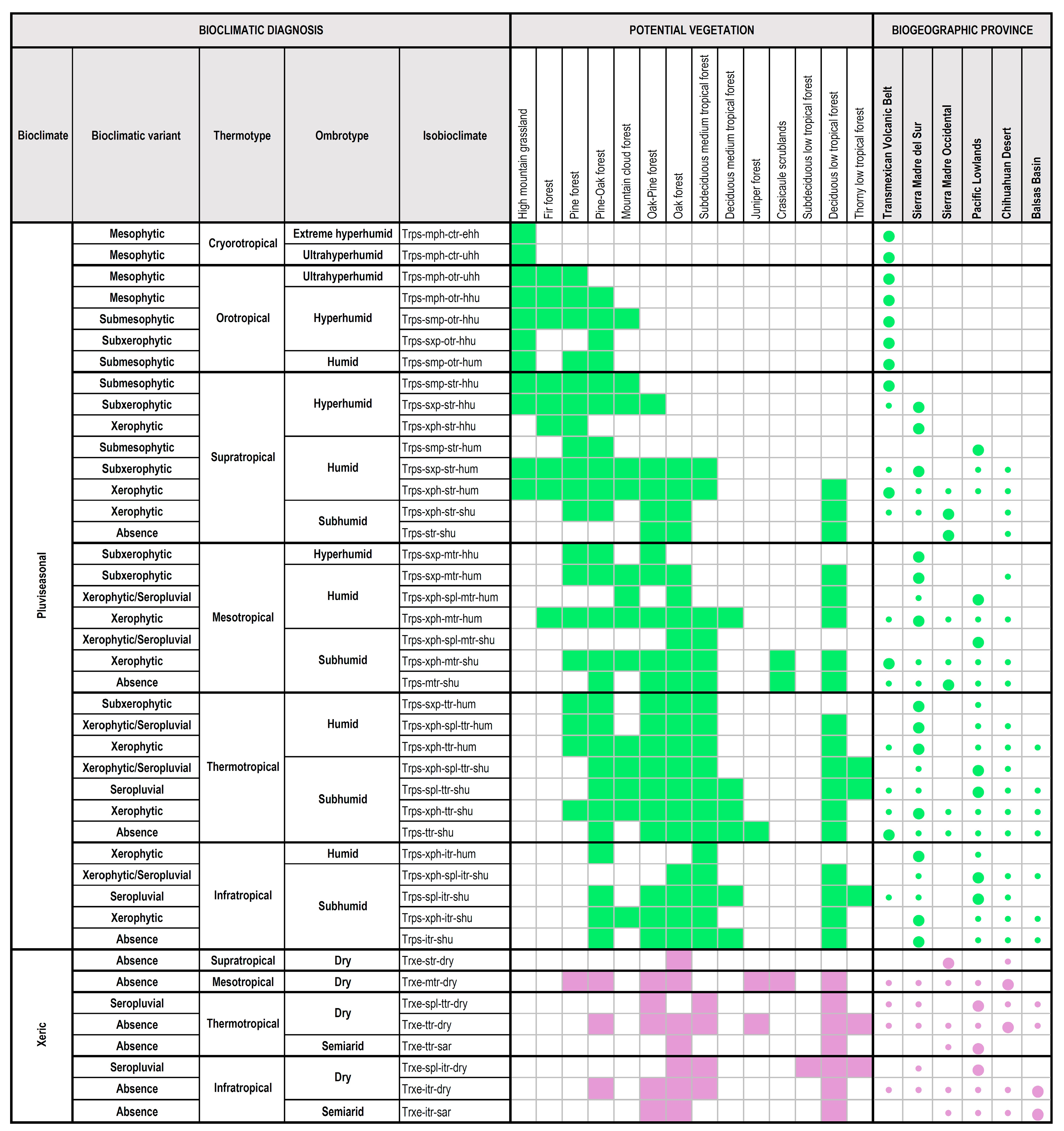
3.2. Correlation Between the Isobioclimates and the Climatophyllous Potential Vegetation

After obtaining the bioclimatic characterization of the study area and creating the corresponding cartography, an analysis was performed to establish the correspondence between isobioclimates and the potential vegetation. This examination focused on the units considered significant indicators for identifying climatophyllous vegetation in INEGI [46]. Consequently, a distinct type of climatophyllous potential vegetation was assigned to each isobioclimate. The distribution of the Trps isobioclimates is associated with territories where the Io is greater than 3.6 and the Iod₂ is less than or equal to 2.5. On the other hand, the Trxe isobioclimates are linked to territories where the Io ranges from 1.0 to 3.6. Figure 8 provides a visual representation of how the identified types of climatophyllous potential vegetation in the study area correspond to the isobioclimatic regions delineated in the study.

The isobioclimates mainly associated with the TVB province include the Trps-mph-ctr-ehh, Trps-mph-ctr-uhh, Trps-mph-otr-uhh, Trps-mph-otr-hhu, Trps-smp-otr-hhu, Trps-sxp-otr-hhu, Trps-smp-otr-hum, Trps-smp-str-hhu, Trps-xph-str-hum, Trps-xph-mtr-shu, and Trps-ttr-shu. The findings indicate that these 11 isobioclimates are primarily linked to high mountain grassland, fir forest, pine forest, pine–oak forest, and mountain cloud forest. Furthermore, correlations were also observed with oak–pine forest, oak forest, subdeciduous medium tropical forest, crasicaule scrubland, and deciduous low tropical forest.

The isobioclimates primarily related to the SMS province encompass the Trps-sxp-str-hhu, Trps-xph-str-hhu, Trps-sxp-str-hum, Trps-sxp-mtr-hhu, Trps-sxp-mtr-hum, Trps-xph-mtr-hum, Trps-sxp-ttr-hum, Trps-xph-spl-ttr-hum, Trps-xph-ttr-hum, Trps-xph-ttr-shu, Trps-xph-itr-hum, Trps-xph-itr-shum, and Trps-itr-shu. The findings reveal that these 13 isobioclimates are predominantly linked to pine forest, pine-oak forest, mountain cloud forest, oak-pine forest, oak forest, subdeciduous medium tropical forest, and deciduous low tropical forest. Additionally, fir forests, and subdeciduous low tropical forests have also been associated with these isobioclimates.

The SMO province is found to be primarily correlated with the Trps-xph-str-shu, Trps-str-shu, Trps-mtr-shu, and Trxe-str-dry. The results indicated a correlation between the four isobioclimates and pine–oak forest, oak–pine forest, and oak forest. However, other climatophyllous potential vegetation types were identified that establish relationships between these isobioclimates, such as the pine forest, crasicaule scrubland, and deciduous low tropical forest.

The PL province is primarily linked to the Trps-smp-str-hum, Trps-xph-spl-mtr-hum, Trps-xph-spl-mtr-shu, Trps-xph-spl-ttr-shu, Trps-spl-ttr-shu, Trps-xph-spl-itr-shu, Trps-spl-itr-shu, Trxe-spl-ttr-dry, Trxe-ttr-sar, and Trxe-spl-itr-dry. Nevertheless, the findings revealed these ten isobioclimates form connections with the oak forest, subdeciduous medium tropical forest, deciduous low tropical forest, and thorny low tropical forest. Furthermore, correlations were observed among various other types of potential vegetation, including the mountain cloud forest, pine forest, pine-oak forest, oak-pine forest, deciduous medium tropical forest, and subdeciduous low tropical forest.

A further province situated in the area corresponds with the CD, which is mainly associated with the Trxe-mtr-dry and Trxe-ttr-dry. In terms of the outcomes obtained, it was found that these two isobioclimates are primarily correlated with the pine–oak forest, oak–pine forest, oak forest, juniper forest, and deciduous low tropical forest. Nevertheless, additional relationships were recognized between the subdeciduous medium tropical forest, crasicaule scrublands, and thorny low tropical forest.

In the case of the BB province, the isobioclimates that are predominantly associated are the Trxe-itr-dry, and Trxe-itr-sar. The results indicated that there are correlations between the two isobioclimates and the pine–oak forest, oak–pine forest, oak forest, subdeciduous medium tropical forest, and deciduous low tropical forest. Figure 9 provides a visual representation of the previously mentioned relationships between the types of potential vegetation and the isobioclimates, as well as their distribution according to the biogeographic provinces.

It is noteworthy that all these relationships have been established based on the information indicated here. However, further investigation is necessary to elucidate the nuances of these relationships, particularly regarding the floristic component, which plays an instrumental role in differentiating exceptional situations and adjusting the reciprocity between potential vegetation and isobioclimates. Figure 9 presents a visual representation of the correlation between climatophyllous potential vegetation and isobioclimates, with the most distribution observed in the state of Jalisco.

4. Discussion

This study is based on the findings of previous research conducted in proximate territories with wide altitudinal gradients. This includes studies by Giménez and Escamilla [32], Barber and Crespo [70], Macías-Rodríguez [28], Giménez and González [67], Peinado et al. [29], Giménez et al. [30], Macías-Rodríguez et al. [8,22], Medina-García et al. [33,34], Ochoa-Ramos [31], and Gopar-Merino et al. [9]. These studies have been based on the bioclimatic methodology, which was employed to identify the relationship between the bioclimatic units and the distribution of climatophyllous potential vegetation. However, most studies conducted in Mexico have employed a phytosociological and vegetational approach, which provides detailed information on the botanical aspect but offers few insights into the bioclimatological characteristics. The present study aims to address this gap by integrating high-resolution climate data, spatial modeling techniques, and geostatistical analyses to establish the foundation for a preliminary bioclimatic characterization of Jalisco. The integration of Geographic Information System (GIS) tools with raster-based spatial analysis ensures a more precise delineation of bioclimatic units. This methodological refinement facilitates a comprehensive bioclimatic diagnosis and enhances the applicability of these classifications in vegetation studies, land management, and ecological assessments under changing climatic conditions.

In comparison to previous bioclimatic studies in Mexico, including those by Giménez et al. [30], Macías-Rodríguez et al. [8], and Gopar-Merino et al. [9], which utilized climate data from weather stations, the present study has obtained the climate data from the global database CHELSA v2.1 with a grid of less than 1 km (0.88 km) [13,56]. The findings of this study corroborate those of some of the previously cited investigations and those of Rivas-Martínez et al. [7], which documented that the study area is situated within the Tropical macrobioclimate. The area includes zonobiomes II (tropical vegetation with summer rainfall) and X (alpine mountain vegetation) [3,28].

Two distinct bioclimates are identified within the area, the Trps (Io ≥ 3.6 and Iod₂ < 2.5) and the Trxe (1.0 < Io ≤ 3.6). This is consistent with the results obtained in previous studies [8,30,31]. The results of the bioclimatic diagnosis revealed the existence of six thermotypes and seven ombrotypes within the study area. These ranged from itr to ctr and from the sar to ehh, respectively. These bioclimatic belts correspond to elevations ranging from sea level to the highest peaks (Nevado de Colima), which is consistent with the findings of Giménez de Azcárate and Escamilla [32], Giménez de Azcárate et al. [71], Almeida-Leñero et al. [72], Giménez de Azcárate and Ramírez [73], Almeida et al. [74], and Macías-Rodríguez et al. [8]. However, none of these works have taken into consideration the bioclimatic variants and levels of continentality. In our study, it was, thus, possible to identify the spl bioclimatic variant in both bioclimates, while the tropical drought bioclimatic variant was exclusive to the Trps bioclimate. In such cases, fluctuations or rhythms in precipitation play a crucial role in the composition and distribution of plant communities. Moreover, the simple continentality index was considered, and their levels recognized in the study area were observed from the southwest to the east of the state, extending from the ultrahyperoceanic weak level on the Pacific coast to the subhyperoceanic strong level in the southern regions of the CD province. The present study represents a novel approach to the consideration of this index in Mexico, with the objective of identifying its levels and classifying the bioclimates. This constitutes a significant contribution to the field, given the crucial influence this index has on the distribution of vegetation. The findings may facilitate the establishment of a correlation between the bioclimates and the grouping of certain types of vegetation.

The heterogeneous nature of the territory and the convergence of several biogeographic provinces in this area have resulted in the identification of a total of 42 distinct isobioclimates. A comparison of these results with those obtained by Macías-Rodríguez et al. [22], in which 19 different isobioclimates for the SMO province were recognized, indicates that the study area is smaller than that SMO province. Additionally, the province has a greater latitudinal range, resulting in the observation of one bioclimate that is not represented in our study, the Tropical desert bioclimate with the thermotropical arid belt. The Trxe bioclimate exhibits a supratropical semiarid belt that is not evident in our study area. This is probably due to the extent and geographical location of the SMO province, particularly in relation to its latitudinal range. The semiarid and arid ombrotypes are primarily associated with the CD province, which is situated from the north to the center of the country. However, our study recognizes the itr-sar belt, which is not evident in the mentioned study; this discrepancy may be attributed to the definition of the climate database utilized. The Trps bioclimate was identified based on the bioclimatic diagnosis, which revealed the presence of otr-hum, otr-hhu, otr-uhh, ctr-uhh, and ctr-ehh belts. These were observed at the highest elevation in the study area, in the Nevado de Colima (4260 m asl). It is worthy of note that a study conducted by Medina García et al. [34], in the Tancítaro massif, located in the state of Michoacán (Mexico) at an elevation of 3840 m asl, reveled the existence of the str and otr thermotypes, and hum and hhu ombrotypes. On the other hand, these findings are consistent with those reported in previous studies, including those by Giménez et al. [30] and Macías-Rodríguez et al. [22]. These studies observed that the limited number of meteorological stations and the marginal positions of these bioclimatic belts made their interpretation challenging. Therefore, our results significantly contribute to the indication that the CHELSA v2.1 database [56], provides greater precision in recognizing these bioclimatic belts.

The relationship between climate and vegetation has been the main focus of many studies using different methodological approaches. In this study, the Worldwide Bioclimatic Classification System by Rivas-Martínez et al. [7] was utilized to analyze the spatial distribution of potential vegetation in Jalisco, Mexico. The main bioclimatic units and their associations with climatophyllous vegetation types were identified. These biophysical models have demonstrated a high level of reciprocity in the relationship between climate and vegetation, which is making possible the creation of bioclimatic and biogeographical maps of the world that are significantly more precise. The current results confirm previous investigation, for example, a study conducted by Giménez et al. [30] at the SMO province, which showed strong correlations between bioclimatic conditions and potential vegetation distribution. This was demonstrated by an analysis of the bioclimatic diagnosis of the weather stations and the flora and vegetation data from the region. The analysis demonstrated a significant correlation between the Trps-mtr-shu isobioclimate and mixed pine and oak forests, as well as the Trxe-ttr-dry isobioclimate and tropical deciduous forests. These two isobioclimates are the most representative in our study area. In terms of methodology, one consideration is the integration of different spatial resolutions in our dataset. The INEGI land use and vegetation layer (1:250,000) [46] provides essential information on vegetation structure and physiognomy but differs in scale from the CHELSA climate data (0.88 km resolution) [56]. This may limit the precision of the correlation between vegetation types and bioclimatic units. However, the use of high-resolution climate data improves the ability to capture microclimatic variability, which is crucial for defining bioclimatic borders. Future studies could refine these correlations by incorporating fine-scale vegetation data or remote sensing techniques to enhance the accuracy of vegetation–climate relationships. Moreover, the correlation between a specific isobioclimate and one or more types of potential vegetation is presented, along with the results obtained in the present study. These findings are also consistent with the results of a recent investigation conducted by Gopar-Merino et al. [9] in the Laguna de Sayula sub-basin. The study demonstrated the reciprocity relationships between isobioclimates and potential vegetation along an altitudinal gradient. The cited investigation addressed floristic indicators. It is, thus, assumed that the floristic indicators will correspond with the already described isobioclimates, thereby demonstrating the efficacy of the methodology proposed by Rivas-Martínez et al. [7]. This methodology highlights one of its fundamental principles, the reciprocity between bioclimates, vegetation series, and biogeographic territories [75].

5. Conclusions

The integrated knowledge of the distribution of potential vegetation and the bioclimatic diagnosis will facilitate the clarification of the relationship between the bioclimatic belts and their corresponding vegetation belts. The present research is open to further geobotanical, ecological, and bioclimatic research, particularly with a focus on floristic and vegetational characteristics, which facilitates the identification of climacic domains within potential vegetation types. In this sense, the detail of the results obtained will allow for the adjustment of the link between the units found here and the changes in the structure, physiognomy, and composition of the potential vegetation in future investigations. Moreover, the variations in the climatic gradient of the territory, reflected in the different parameters of bioclimatic approximation applied, will be of great value in the identification of such changes, as well as in the incorporation of other variables of geographic and geomorphological character that will help to nuance and adjust the general model of bioclimatic reciprocity presented here. The value of studies such as this resides in their utility as a foundation for accurately correlating vegetation studies with a focus on management and territorial planning in light of changes due to global warming and other environmental issues of relevance. This study provides essential insights for territorial planning by identifying the bioclimatic conditions that influence the distribution of potential vegetation types. Understanding these relationships is fundamental to developing effective land management strategies, conservation planning, and ecological restoration initiatives. The results can help to delineate areas of high conservation value, improve land use regulations, and guide reforestation or planting programs based on bioclimatic suitability. In light of the increasing pressures of climate change, the bioclimatic classification proposed in this study offers a predictive framework to evaluate its potential impact on vegetation dynamics. This framework facilitates the development of proactive adaptation and mitigation measures, ensuring that conservation and management efforts are aligned with future climatic scenarios. The significance of this approach resides in its ability to integrate vegetation studies with territorial planning, providing a scientific foundation for sustainable environmental management. By enhancing our comprehension of climate–vegetation interactions, this research promotes the formulation of policies and initiatives centered on the restoration and conservation of natural ecosystems. Subsequent studies should extend this bioclimatic framework by incorporating functional trait analyses and ecological dynamics, thereby further enhancing its relevance in geobotanical and ecological research.

References

1. Box, E. Macroclimate and Plant Forms: An Introduction to Predictive Modelling in Phytogeography; Springer: Dordrecht, The Netherlands, 1981; ISBN 978-94-009-8682-4. [Google Scholar]
2. Troll, C. Seasonal Climates of the Earth. In Weltkarten zur Klimakunde/World Maps of Climatology; Springer: Berlin/Heidelberg, Germany, 1965; pp. 19–25. ISBN 978-3-662-13419-1. [Google Scholar]
3. Walter, H. Vegetation of the Earth and Ecological Systems of the Geo-Biosphere; Heidelberg Science Library; Springer: Berlin/Heidelberg, Germany, 1985; ISBN 978-3-540-13748-1. [Google Scholar]
4. Woodward, F.I. Climate and Plant Distribution; Cambridge University Press: Cambridge, UK, 1987; ISBN 978-052-1282147. [Google Scholar]
5. Navarro, G.; Maldonado, M. Geografía Ecológica de Bolivia. Vegetación y Ambientes Acuáticos; Centro de Ecología Simón I: Cochabamba, Bolivia, 2002; ISBN 99905-0-2250. [Google Scholar]
6. Larcher, W. Physiological Plant Ecology; Springer: Berlin/Heidelberg, Germany, 2003; ISBN 3-540-43516-6. [Google Scholar]
7. Rivas-Martínez, S.; Rivas Sáenz, S.; Penas, Á. Worldwide Bioclimatic Classification System. Glob. Geobot. 2011, 1, 1–634. [Google Scholar]
8. Macías-Rodríguez, M.Á.; Peinado Lorca, M.; Giménez de Azcárate, J.; Aguirre Martínez, J.L.; Delgadillo Rodríguez, J. Clasificación Bioclimática de La Vertiente Del Pacífico Mexicano y Su Relación Con La Vegetación Potencial. Acta Bot. Mex. 2014, 109, 133–165. [Google Scholar] [CrossRef]
9. Gopar-Merino, L.F.; Macías-Rodríguez, M.Á.; Giménez de Azcárate, J. Bioclimatology, Floristic Indicators and Potential Vegetation of the Sayula Sub-Basin, Jalisco, México. Bot. Sci. 2022, 100, 877–898. [Google Scholar] [CrossRef]
10. Walter, H. Zonas de Vegetación y Clima. Breve Exposición Desde El Punto de Vista Causal y Global; Omega: Barcelona, España, 1997; ISBN 9788428203104. [Google Scholar]
11. Breckle, S.W. Walter’s Vegetation of the Earth; Springer: Berlin/Heidelberg, Germany, 2002; ISBN 978-3-540-43315-6. [Google Scholar]
12. Livneh, B.; Bohn, T.J.; Pierce, D.W.; Munoz-Arriola, F.; Nijssen, B.; Vose, R.; Cayan, D.R.; Brekke, L. A Spatially Comprehensive, Hydrometeorological Data Set for Mexico, the U.S., and Southern Canada 1950–2013. Sci. Data 2015, 2, 150042. [Google Scholar] [CrossRef]
13. Karger, D.N.; Conrad, O.; Böhner, J.; Kawohl, T.; Kreft, H.; Soria-Auza, R.W.; Zimmermann, N.E.; Linder, H.P.; Kessler, M. Climatologies at High Resolution for the Earth’s Land Surface Areas. Sci. Data 2017, 4, 170122. [Google Scholar] [CrossRef]
14. Hernández Cerda, M.E.; Ordoñez Díaz, M.D.J.; Giménez de Azcárate, J. Comparative Analysis of Two Bioclimatic Classification Systems in Mexico. Investig. Geográficas 2018, 95, 1–14. [Google Scholar] [CrossRef]
15. Cuadrat, J.M.; Pita, M.F. Climatología; Ediciones Cátedra, Geografía: Madrid, España, 2006; ISBN 9788437615318. [Google Scholar]
16. Tuhkanen, S. Climatic Parameters and Indices in Plant Geography; Acta Phytogeographica Suecica: Uppsala, Sweden, 1980; Volume 67, ISBN 91-7210-067-2. [Google Scholar]
17. Müller, M.J. Selected Climatic Data for a Global Set of Standard Stations for Vegetation Science; Tasks for vegetation science; Springer: Dordrecht, The Netherlands, 1982; Volume 5, ISBN 978-94-009-8042-6. [Google Scholar]
18. Sayre, R.; Yanosky, A.; Muchoney, D. Mapping Global Ecosystems; The GEOSS Global Earth Observation System of Systems Approach, in Group on Earth Observations Secretariat. Available online: https://www.earthobservations.org/index.php (accessed on 7 February 2023).
19. Cress, J.J.; Sayre, R.; Comer, P.; Warner, H. Terrestrial Ecosystems—Isobioclimates of the Conterminous United States; U.S. Geological Survey Scientific: Reston, VA, USA, 2009; Investigations Map 3084, Scale 1:5,000,000, 1 Sheet 2009. [Google Scholar]
20. Peinado, M.; Macías-Rodríguez, M.Á.; Aguirre, J.L.; Delgadillo Rodríguez, J. Bioclimate-Vegetation Interrelations in Northwestern Mexico. Southwest Nat. 2010, 55, 311–322. [Google Scholar] [CrossRef]
21. Gopar-Merino, L.F.; Velázquez, A. Landscape Components as Predictors of Vegetation Coverage: The Study Cases of the State of Michoacán, México. Investig. Geográficas 2016, 90, 75–88. [Google Scholar] [CrossRef]
22. Macías-Rodríguez, M.Á.; Giménez de Azcárate-Cornide, J.; Gopar-Merino, L.F. Bioclimatic Systematization of Sierra Madre Occidental (Mexico) and It’s Relationship with Vegetation Belts. Polibotanica 2017, 43, 125–163. [Google Scholar] [CrossRef]
23. Gopar-Merino, L.F.; Velázquez, A.; Giménez de Azcárate, J. Bioclimatic Mapping as a New Method to Assess Effects of Climatic Change. Ecosphere 2015, 6, 1–12. [Google Scholar] [CrossRef]
24. Peinado, M.; Aguirre, J.L.; Delgadillo, J. Phytosociological, Bioclimatic and Biogeographical Classification of Woody Climax Communities of Western North America. J. Veg. Sci. 1997, 8, 505–528. [Google Scholar] [CrossRef]
25. Peinado, M.; Bartolome, C.; Delgadillo, J.; Aguado, I. Pisos de Vegetación de La Sierra de San Pedro Mártir, Baja California, México. Acta Bot. Mex. 1994, 29, 1–30. [Google Scholar] [CrossRef]
26. Peinado, M.; Alcaraz, F.; Aguirre, J.L.; Martínez-Parras, J. Vegetation Formations and Associations of the Zonobiomes along the North American Pacific Coast: From Northern California to Alaska. Plant Ecol. 1997, 129, 29–47. [Google Scholar] [CrossRef]
27. Peinado, M.; Aguirre, J.L.; Delgadillo, J.; Macías, M.Á. Zonobiomes, Zonoecotones and Azonal Vegetation along the Pacific Coast of North America. Plant Ecol. 2007, 191, 221–252. [Google Scholar] [CrossRef]
28. Macías-Rodríguez, M.Á. Estudio de Las Relaciones Entre Zonobiomas, Bioclimas y Vegetación En La Costa Del Pacífico Norteamericano. Ph.D. Thesis, Universidad de Alcalá, Madrid, Spain, 2009. [Google Scholar]
29. Peinado, M.; Macías, M.Á.; Ocaña-Peinado, F.M.; Aguirre, J.L.; Delgadillo, J. Bioclimates and Vegetation along the Pacific Basin of Northwestern Mexico. Plant Ecol. 2011, 212, 263–281. [Google Scholar] [CrossRef]
30. Giménez de Azcárate, J.; Macías Rodríguez, M.Á.; Gopar Merino, F. Bioclimatic Belts of Sierra Madre Occidental (Mexico): A Preliminary Approach. Int. J. Geobot. Res. 2013, 3, 19–35. [Google Scholar] [CrossRef]
31. Ochoa-Ramos, N.Y. Clasificación Bioclimática Del Occidente de México y Su Relación Con La Vegetación Potencial; Universidad de Guadalajara: Jalisco, México, 2020. [Google Scholar]
32. Giménez de Azcárate, J.; Escamilla, M. Las Comunidades Edafoxerófilas (Enebrales y Zacatonales) En Las Montañas Del Centro de México. Phytocoenologia 1999, 29, 449–468. [Google Scholar]
33. Medina-García, C.; Velázquez, A.; Giménez de Azcárate, J.; Macías-Rodríguez, M.Á.; Larrazábal, A.; Gopar-Merino, L.F.; López-Barrera, F.; Pérez-Vega, A. Phytosociology of a Seasonally Dry Tropical Forest in the State of Michoacán, Mexico. Bot. Sci. 2020, 98, 441–467. [Google Scholar] [CrossRef]
34. Medina García, C.; Gimenez de Azcarate, J.; Velázquez Montes, A. Las Comunidades Vegetales Del Bosque de Coníferas Altimontano En El Macizo Del Tancítaro (Michoacán, México). Acta Bot. Mex. 2020. [Google Scholar] [CrossRef]
35. Villaseñor, J.L. Checklist of the Native Vascular Plants of Mexico. Rev. Mex. Biodivers 2016, 87, 559–902. [Google Scholar] [CrossRef]
36. Morrone, J.J.; Escalante, T.; Rodríguez-Tapia, G. Mexican Biogeographic Provinces: Map and Shapefiles. Zootaxa 2017, 4277, 277–279. [Google Scholar] [CrossRef] [PubMed]
37. Sayre, R.; Brow, J.; Josse, C.; Sotomayor, L.; Touval, J. Terrestrial Ecosystems of South America. In North America Land Cover Summit; Association of American Geographers: Washington, DC, USA, 2008; pp. 131–152. [Google Scholar]
38. Sayre, R.; Comer, P.; Warner, H.; Cress, J. A New Map of Standardized Terrestrial Ecosystems of the Conterminous United States: Professional Paper 1768; U.S. Geological Survey: Washington, DC, USA, 2009; p. 17. ISBN 978-1-4113-2432-9. [Google Scholar]
39. Sayre, R.G.; Comer, P.; Hak, J.; Josse, C.; Bow, J.; Warner, H.; Larwanou, M.; Kelbessa, E.; Bekele, T.; Kehl, H. A New Map of Standardized Terrestrial Ecosystems of Africa; Association of American Geographers: Washington, DC, USA, 2013; p. 24. ISBN 978-0-89291-275-9. [Google Scholar]
40. Amigo, J.; Ramírez, C. A Bioclimatic Classification of Chile: Woodland Communities in the Temperate Zone. Plant Ecol. 1998, 136, 9–26. [Google Scholar]
41. INEGI Carta Del Marco Geoestadístico. Escala 1:4,000,000 2020. Available online: https://www.inegi.org.mx/app/mapas/ (accessed on 7 February 2023).
42. INEGI Carta Hidrográfica. Escala 1:250,000 2006. Available online: https://www.inegi.org.mx/app/mapas/ (accessed on 7 February 2023).
43. Valdivia-Ornelas, L.; Castillo-Aja, M.R. Las Regiones Geomorfológicas Del Estado de Jalisco. Rev. Geocalli 2001, 2, 17–108. [Google Scholar]
44. Espinosa Organista, D.; Ocegueda Cruz, S. El Conocimiento Biogeográfico de Las Especies y Su Regionalización Natural. Cap. Nat. México 2008, 1, 33–65. [Google Scholar]
45. Guía Para La Interpretación de Cartografía: Uso de Suelo y Vegetación; Escala 1:250,000, Serie VI; INEGI: Aguascalientes, México, 2017.
46. Conjunto de Datos Vectoriales de Uso de Suelo y Vegetación; Escala 1:250,000, Serie VII, Conjunto Nacional; INEGI: Aguascalientes, México, 2021.
47. Ruiz-Corral, J.A.; Contreras Rodriguez, S.H.; García Romero, G.E.; Villavicencio García, R. Climates of Jalisco According to the Köppen-García System with Adjustment for Potential Vegetation. Rev. Mex. Cienc. Agrícolas 2021, 12, 805–821. [Google Scholar]
48. Morrone, J.J. Neotropical Biogeography; CRC Press: Boca Raton, FL, USA, 2017; ISBN 9781315390666. [Google Scholar]
49. Gámez, N.; Escalante, T.; Rodríguez, G.; Linaje, M.; Morrone, J.J. Caracterización Biogeográfica de La Faja Volcánica Transmexicana y Análisis de Los Patrones de Distribución de Su Mastofauna. Rev. Mex. Biodivers 2012, 83, 258–272. [Google Scholar] [CrossRef]
50. Rzedowski, J. Vegetación de México; Limusa: Ciudad de México, Mexico, 1978; ISBN 968-1800028. [Google Scholar]
51. Dinerstein, E.; Olson, D.M.; Graham, D.J.; Webster, A.L.; Primm, S.A.; Bookbinder, M.P.; Ledec, G. Una Evaluación Del Estado de Conservación de Las Ecorregiones Terrestres de América Latina y El Caribe; World Bank: Washington, DC, USA, 1995; ISBN 0-8213-3296-1. [Google Scholar]
52. Luna-Vega, I.; Espinosa, D.; Contreras-Medina, R. Biodiversidad de La Sierra Madre Del Sur: Una Síntesis Preliminar; UNAM: Ciudad de México, Mexico, 2016; ISBN 978-6070279065. [Google Scholar]
53. Morrone, J.J. Biogeographic Regionalization and Biotic Evolution of Mexico: Biodiversity’s Crossroads of the New World. Rev. Mex. Biodivers 2019, 90, 1–68. [Google Scholar] [CrossRef]
54. Linares-Palomino, R.; Oliveira-Filho, A.T.; Pennington, R.T. Neotropical Seasonally Dry Forests: Diversity, Endemism, and Biogeography of Woody Plants. In Seasonally Dry Tropical Forests; Island Press/Center for Resource Economics: Washington, DC, USA, 2011; pp. 3–21. [Google Scholar]
55. Cabrera, A.L.; Willink, S.E. Biogeografía de América Latina; OEA: Washington, DC, USA, 1973; Volume 13. [Google Scholar]
56. Karger, D.N.; Conrad, O.; Böhner, J.; Kawohl, T.; Kreft, H.; Soria-Auza, R.W.; Zimmermann, N.E.; Linder, H.P.; Kessler, M. Climatologies at High Resolution for the Earth’s Land Surface Areas. EnviDat 2021. [Google Scholar] [CrossRef]
57. Dee, D.P.; Uppala, S.M.; Simmons, A.J.; Berrisford, P.; Poli, P.; Kobayashi, S.; Andrae, U.; Balmaseda, M.A.; Balsamo, G.; Bauer, P.; et al. The ERA-Interim Reanalysis: Configuration and Performance of the Data Assimilation System. Q. J. R. Meteorol. Soc. 2011, 137, 553–597. [Google Scholar] [CrossRef]
58. Bland, J.M.; Altman, D.G. Measuring Agreement in Method Comparison Studies. Stat Methods Med. Res. 1999, 8, 135–160. [Google Scholar] [CrossRef]
59. Rivas-Martínez, S.; Lousã, M.; Costa, J.C.; Duarte, M.C. Geobotanical Survey of Cabo Verde Island (West Africa). Int. J. Geobot. Res. 2017, 7, 1–103. [Google Scholar]
60. Esri ArcGIS PRO; Esri: Redlands, CA, USA, 2023.
61. González, M.; Hernández Xolocotzi, E. Los Tipos de Vegetación de México y Su Clasificación. Bot. Sci. 1963, 28, 29–179. [Google Scholar] [CrossRef]
62. Pennington, T.D.; Sarukhán, J. Árboles Tropicales de México; Fondo de Cultura Económica: Ciudad de México, México, 1998; ISBN 970-32-1643-9. [Google Scholar]
63. González Medrano, F. Las Comunidades Vegetales de México; Segunda edición; INE-SEMARNAT: Ciudad de México, México, 2004; ISBN 968-817-611-7. [Google Scholar]
64. Challenger, A.; Soberón, J. Los Ecosistemas Terrestres, En Capital Natural de México. In Vol I: Conocimiento actual de la Biodiversidad; CONABIO, Ed.; CONABIO: Ciudad de México, México, 2008; pp. 87–108. [Google Scholar]
65. Villaseñor, J.L.; Ortiz, E. Biodiversidad de Las Plantas Con Flores (División Magnoliophyta) En México. Rev. Mex. Biodivers 2014, 85, 134–142. [Google Scholar] [CrossRef]
66. Flores Mata, G.; Jiménez, L.; Madrigal, S.; Takaki, T. Tipos de Vegetación de La República Mexicana; Secretaría de Recursos Hidráulicos: Ciudad de México, México, 1971. [Google Scholar]
67. Giménez de Azcárate, J.; González Costilla, O. Pisos de Vegetación de La Sierra de Catorce y Territorios Circundantes (San Luis Potosí, México). Acta Bot. Mex. 2011, 94, 91–123. [Google Scholar]
68. García, E. Modificaciones al Sistema de Clasificación Climática de Köppen; Instituto de Geografía/Universidad Nacional Autónoma de México: Ciudad de México, México, 1998; Volume 6, ISBN 970-32-1010-4. [Google Scholar]
69. Martinez, S.R.; Aguiar, C.; Aguilella, A.; Alonso, R.; Alvarez, M.; Amich, F.; Arnaiz, C.; Baccheta, G.; Barbero, M.; Barbour, M.G.; et al. Map of Series, Geoseries and Geopermaseries of Vegetation in Spain. Itinera Geobot. 2007, 17, 5–436. [Google Scholar]
70. Barber, A.; Tun, J.; Crespo, B. A New Approach on the Bioclimatology and Potential Vegetation of the Yucatan Peninsula (Mexico). Phytocoenologia 2001, 31, 1–31. [Google Scholar]
71. Giménez de Azcárate, J.; Ramírez, M.I.; Pinto, M. Las Comunidades Vegetales de La Sierra de Angangueo (Estados de Michoacán y México, México): Clasificación, Composición y Distribución. Lazaroa 2003, 24, 87–111. [Google Scholar]
72. Almeida-Leñero, L.; Giménez de Azcárate, J.; Cleef, A.; González Trápaga, A. Las Comunidades Vegetales Del Zacatonal Alpino de Los Volcanes Popocatépetl y Nevado de Toluca, Región Central de México. Phytocoenologia 2004, 34, 91–132. [Google Scholar] [CrossRef]
73. Giménez de Azcárate, J.; Ramírez, M.I. Análisis Fitosociológico de Los Bosques de Oyamel [Abies Religiosa (H.B.K.) Cham. & Schlecht.] de La Sierra de Angangueo, Región Central de México. Fitosociologia 2004, 41, 91–100. [Google Scholar]
74. Almeida, L.; Escamilla, M.; Giménez de Azcárate, J.; González, A.; Cleef, A. La Vegetación Alpina de Los Volcanes Popocatépetl, Iztacíhuatl y Nevado de Toluca. In Biodiversidad de la Faja Volcánica Transmexicana; FES Zaragoza-CONABIO: Ciudad de México, México, 2007; pp. 179–198. [Google Scholar]
75. del Río, S. El Cambio Climático y Su Influencia En La Vegetación de Castilla y León (España). Itinera Geobot. 2005, 16, 5–534. [Google Scholar]
Figure 1. Administrative delimitation, bordering states, and highest elevation of the study area.
Remotesensing 17 01232 g001
Figure 2. Spatial distribution of recognized bioclimates in the state of Jalisco.
Remotesensing 17 01232 g002
Figure 3. Spatial distribution of the bioclimates and bioclimatic variants identified in the state of Jalisco. Acronyms: Trps = Tropical pluviseasonal, Trxe = Tropical xeric, spl = seropluvial, xph = xerophytic, sxp = subxerophytic, smp = submesophytic, mph = mesophytic.
Remotesensing 17 01232 g003
Figure 4. Spatial distribution of the bioclimates and levels of simple continentality recognized in the state of Jalisco. Acronyms: Trps = Tropical pluviseasonal, Trxe = Tropical xeric, uhow = ultrahyperoceanic weak, ehos = euhyperoceanic strong, ehow = euhyperoceanic weak, shos = subhyperoceanic strong.
Remotesensing 17 01232 g004
Figure 5. Spatial distribution of recognized thermotypes in the state of Jalisco.
Remotesensing 17 01232 g005
Figure 6. Spatial distribution of recognized ombrotypes in the state of Jalisco.
Remotesensing 17 01232 g006
Figure 7. Spatial distribution of the basic isobioclimates recognized in the state of Jalisco. Acronyms: Trps = Tropical pluviseasonal, Trxe = Tropical xeric, itr = infratropical, ttr = thermotropical, mtr = mesotropical, str = supratropical, otr = orotropical, ctr = cryorotropical, sar = semiarid, dry = dry, shu = subhumid, hum = humid, hhu = hyperhumid, uhh = ultrahyperhumid, ehh = extreme hyperhumid.
Remotesensing 17 01232 g007
Figure 8. Correspondence between the potential vegetation and the isobioclimates in the state of Jalisco. ● = Biogeographic province in which the isobioclimate is most distributed, • = Other biogeographic provinces where the isobioclimate can be found, green color = Tropical pluviseasonal isobioclimates, purple color = Tropical xeric isobioclimates. Acronyms: Trps = Tropical pluviseasonal, Trxe = Tropical xeric, spl = seropluvial, xph = xerophytic, sxp = subxerophytic, smp = submesophytic, mph = mesophytic, itr = infratropical, ttr = thermotropical, mtr = mesotropical, str = supratropical, otr = orotropical, ctr = cryorotropical, sar = semiarid, dry = dry, shu = subhumid, hum = humid, hhu = hyperhumid, uhh = ultrahyperhumid, ehh = extreme hyperhumid.
Remotesensing 17 01232 g008
Figure 9. Correlation between climatophyllous potential vegetation and isobioclimates with the most distribution in the state of Jalisco. (a) Pine-Oak forest in the Sierra de Mazamitla, and its relationship with the Trps-mtr-shu isobioclimate. (b) Thorny tropical forest in Sayula, and its relationship with the Trxe-ttr-dry isobioclimate. (c) Subdeciduous tropical forest in Mismaloya, and its relationship with the Trps-ttr-shu isobioclimate. (d) Oak forest in Bolaños, and its relationship with the Trxe-mtr-dry isobioclimate. (e) Pine forest in the Nevado de Colima, and its relationship with the Trps-mtr-hum isobioclimate. (f) Deciduous low tropical forest in Bolaños, and its relationship with the Trxe-itr-dry isobioclimate. (g) Oak forest in Bosque La Primavera, and its relationship with the Trps-itr-shu isobioclimate. (h) Mountain cloud forest in Talpa de Allende, and its relationship with the Trps-ttr-hum isobioclimate.
Remotesensing 17 01232 g009