A Fast and Accurate Calculation Method of Water Vapor Transmission: Based on LSTM and Attention Mechanism Model

Abstract

Atmospheric water vapor plays a significant impact on the climate system, radiative transfer models, and optoelectronic engineering applications. Fast and accurate calculation of its optical depth and transmittance is a crucial step to studying the radiation characteristics of water vapor. Although the traditional physics-based, line-by-line radiative transfer model (LBLRTM) meets the accuracy requirements, it is too slow and computationally expensive for practical applications. In this study, to facilitate the accuracy and efficiency requirements of atmospheric water vapor optical depth and transmittance calculation, we propose a Stack LSTM-AT model that combines a double-layer Long Short-Term Memory (LSTM) network and a self-attention mechanism method, and different configurations of the hybrid model are extensively examined. The results show that, compared to the LBLRTM model, the Stack LSTM-AT model significantly improves computational efficiency while maintaining accuracy. Overall, the R-squared, mean absolute error (MAE), and root mean square error (RMSE) of optical depth is 0.9999945, 0.00568, and 0.02033, respectively, while the R-squared, MAE, and RMSE of atmospheric transmittance is 0.9999964, 5.5586 × 10⁻⁴, and 9.4 × 10⁻⁴, respectively. Moreover, the difference in optical depths and transmittance between the prediction results of the Stack LSTM-AT model and the calculation results of the LBLRTM are no greater than 0.3 and 0.008, respectively, across various pressures, temperatures, and water vapor amounts. The computation time for calculating the transmittance of a single spectrum (1–5000 cm⁻¹) is about 9.784 × 10⁻² s, with a spectrum resolution of 1 cm⁻¹, which is about 1000 times faster than that of LBLRTM. The proposed Stack LSTM-AT model could significantly enhance the efficiency and accuracy of atmospheric radiative transfer simulations, demonstrating its broad potential in real-time meteorological monitoring and atmospheric component inversion. This study may provide new insights and technical support for the study of radiative transfer, climate change, and atmospheric environmental monitoring.

1. Introduction

Water vapor is the most influential trace gas in the atmosphere, as it approximately doubles the warming caused by the carbon dioxide alone through positive climate feedbacks [1]. Water vapor changes the global radiation budget by absorbing solar shortwave radiation and terrestrial longwave radiation, having a significant impact on global temperature variations [2]. Additionally, it plays a crucial role in atmospheric climate models and radiative transfer models through cloud-radiative effects and latent heat release [3,4,5]. Therefore, accurately evaluating the radiation characteristics of water vapor is of great significance for further understanding the mechanism of atmospheric radiation transmission [6] and improving the accuracy and reliability of climate models, radiative transfer models, and remote sensing applications.

The Line-by-Line Radiative Transfer Model (LBLRTM) [7] is a highly precise radiative transfer model that accounts for the detailed spectral characteristics of molecular absorption, enabling accurate simulation of the absorption and scattering effects of various molecular species in the atmosphere. However, its computational process is complex and time-consuming [8], requiring substantial computational resources, which limits its practical applications. The LBLRTM is used more often as a benchmark to evaluate the accuracy of other methods [9,10]. To reduce the computational burden caused by excessive integrations in the LBLRTM, several rapid and efficient numerical methods have been developed for remote sensing, climate, and radiative transfer applications, including band models [11,12], statistical regression methods [13,14], spectral sampling strategies [15,16], etc. These models have been widely used in remote sensing, radiative transfer, and climate models. But overall, the computational burden is still heavy; for example, in climate models, radiation calculations can account for up to 50% of all calculations [17]. Even under the conditions of using supercomputers, radiation schemes in weather and climate models can only choose relatively coarse spatial and temporal resolutions to meet the requirements of computational efficiency, which may lead to inevitable deviations in the model when simulating specific weather phenomena or regional radiation conditions, thereby affecting the predictive ability and application effectiveness of the models. Moreover, these methods are complex and cumbersome, posing a high threshold for non-specialists. Therefore, it is crucial to simplify the algorithm for non-specialist researchers while ensuring accuracy and efficiency.

In recent years, with the development of computer technology, various deep learning methods have been widely applied in the study of the parameterization of atmospheric radiative transfer. For example, Alizamir et al. [18] combined wavelet transform with the LSTM (Long Short-Term Memory) model, which significantly improved the accuracy of daily solar radiation forecasting, providing a reliable methodological support for solar energy applications based on climate parameters. Lu et al. [19] developed an efficient and accurate hybrid model by combining radiative transfer models with machine learning models, estimating global solar radiation and quantifying related uncertainties, thus providing scientific support and practical value for large-scale solar radiation estimation. André et al. [20] employed the recurrent neural networks (RNNs) approach to investigate the radiation properties of non-homogeneous gas media. Stegmann et al. [16] proposed replacing the regression coefficients in traditional fast radiative transfer models with deep learning, achieving efficient atmospheric transmittance computation through neural network training, balancing computational speed and accuracy, and offering an innovative solution for operational applications. Chevallier et al. [21] developed the NeuroFlux model using neural networks by inferring parameters from line-by-line and band radiative transfer results based on the TIGR dataset, achieving high-accuracy longwave radiative budget estimation 22 times faster than band models and 106 times faster than line-by-line models. Krasnopolsk et al. [22] implemented their neural network emulation approach for full model radiation in the NCAR CAM, achieving 150 and 20 times speed improvements for longwave and shortwave radiation parameterizations, respectively, with decadal climate simulations yielding nearly identical results to the original model, thereby enabling efficient long-term climate and weather prediction. These studies demonstrate that the application of deep learning methods in the study of atmospheric radiative transfer is continuously expanding, not only improving computational efficiency but also significantly enhancing the accuracy and applicability of models. However, the current fast calculation methods for atmospheric radiative transfer based on deep learning mostly target the specific absorption bands of gases. The required bands may differ for different application scenarios, including remote sensing, military, communication, etc. Hence, it is necessary to construct a combined atmospheric radiative transfer model to adapt to different application requirements.

As a variant of the RNN [23], LSTM demonstrates significant potential in handling tasks involving complex structured data [24]. Researchers used LSTMs to achieve remarkable results in diverse domains, including image recognition [25], classification tasks [26], emotion recognition [27], and fault detection [28]. Additionally, in the field of atmospheric science, LSTM has been increasingly adopted to tackle complex problems. For example, Wang et al. [29] developed an irradiance forecasting method based on the multi-physical process of atmosphere optics and an LSTM-BP model. The results showed higher accuracy compared to the traditional time-series prediction methods under different time scales and weather conditions. Zhao et al. [30] proposed an LSTM-based ERA5 temperature model (LSTM-ERATM), and the results showed that LSTM-ERATM can effectively improve the accuracy of calculating atmospheric weighted mean temperature.

In addition, the attention mechanism enables dynamic weight allocation by focusing on the most relevant parts of the input sequence for the current task, thereby significantly improving the model’s computational speed and accuracy [31]. Compared to the traditional LSTM architecture that processes sequence data recursively through fixed time [32], the introduction of the self-attention mechanism achieves dynamic feature weighting across time steps [33], enhancing the model’s learning efficiency and global feature extraction capability. Consequently, in tasks such as classification [34] or prediction [35], LSTM models integrated with attention mechanisms exhibit superior performance [36,37].

In this study, we propose a novel and efficient water vapor transmittance calculation model, termed the Stack LSTM-AT model, designed to achieve high accuracy and rapid computation of water vapor atmospheric transmittance. The model holds significant potential for applications in diverse fields, including remote sensing, atmospheric radiative transfer, optoelectronic engineering, etc. The main structure of this study is organized as follows: Section 2 introduces the Stack LSTM-AT model and the numerical methods; Section 3 presents the representative results; and Section 4 concludes the study with a summary of our studies and their implications.

2. Materials and Methods

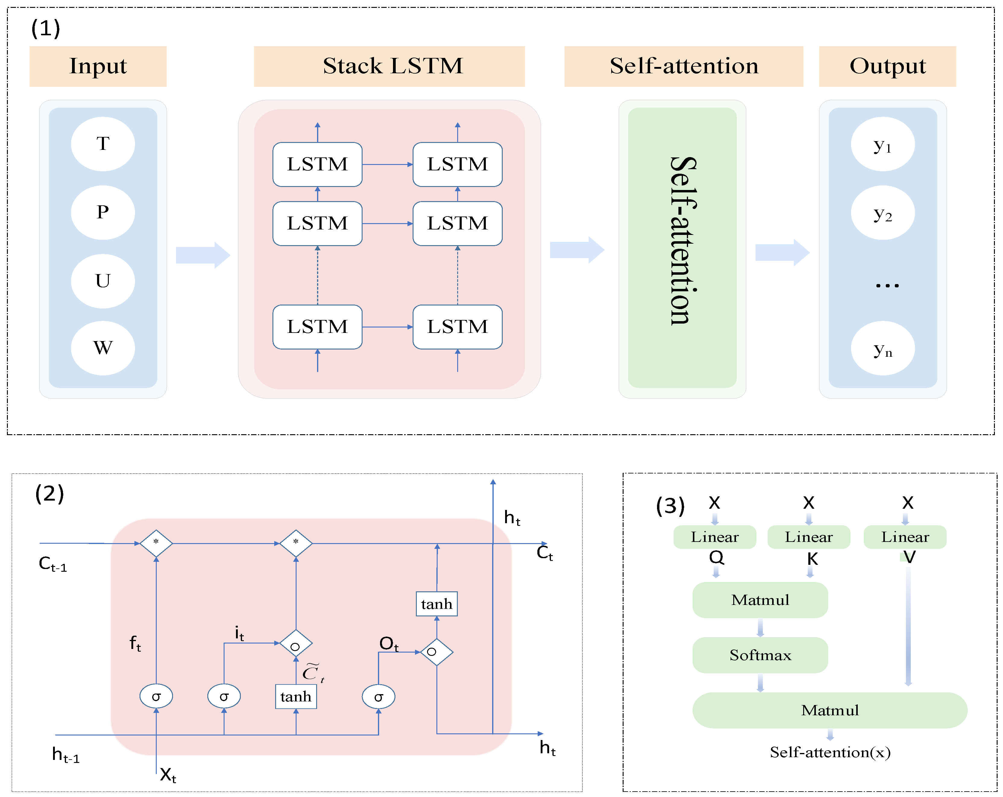
2.1. Stack LSTM-AT Model

The Stack LSTM-AT model proposed in this study is a neural network model that combines a double-layer LSTM structure with a self-attention mechanism, and its overall architecture is shown in Figure 1. LSTM is highly effective in capturing the trend of the relationship within the optical depth, while the self-attention mechanism can enhance the accuracy and stability of the prediction results by focusing the model on the key absorption regions and the interactions between different wavenumbers. In this subsection, the basic structure of the proposed model is explained separately to demonstrate the research value of the model.

2.1.1. Input and Output Module

In this study, the monochromatic optical depths are computed with the LBLRTM using the HITRAN2020 molecular database [38]. The HITRAN2020 database contains detailed molecular absorption information, which is crucial for the study of atmospheric radiation transfer and optical properties. In practical applications, extremely high spectral resolution is not necessary, and a wavenumber interval of 1 cm⁻¹ is generally sufficient. To improve computational efficiency and reduce data volume, we average the high-resolution transmittance data to match the 1 cm⁻¹ wavenumber interval. This approach effectively smooths high-frequency fluctuations while ensuring the results remain within an acceptable error range for practical use. Additionally, previous studies have demonstrated that a resolution of 1 cm⁻¹ is adequate for accurately representing atmospheric transmittance variations, with further details available in reference [39]:

$$\overline{T_v}\left(T,P,U\right)={\displaystyle \frac{{{\displaystyle \int }}_{v-\Delta v/2}^{v+\Delta v/2}exp\left[-k_v\left(T,P\right)U\right]dv}{{{\displaystyle \int }}_{v-\Delta v/2}^{v+\Delta v/2}dv}}$$

(1)

where, $\overline{T_v}$ represents the average transmittance, $k_v$ is the absorption coefficient, $T$ is the temperature, $P$ is the pressure, $U$ is the water vapor amount, and $\Delta v$ is the wavenumber interval width, which is set to 1 cm⁻¹ in this case. Figure 2 shows the comparison between the average optical depth and the original monochromatic optical depth for water vapor in the 3500 to 3520 cm⁻¹ wavenumber range at a pressure of 1200 hPa, a temperature of 200 K, and a water vapor amount of 415 atm-cm. It can be observed that the original monochromatic optical depth exhibits significant peaks and valleys near certain wavenumber points, while the calculated average optical depth follows a much smoother trend.

Since the optical depth of water vapor is related to wavenumber, temperature, pressure, and water vapor amount, this study takes these four parameters as the input features of the neural network model. The data are shown in

Table 1. Specific ranges of parameters.

Variant	Value
T/K	200:410:30
P/hPa	1200.0, 350.0, 100.0, 35.0
U/atm-cm	0.00005:415:0.00005*1.31(i−1)
Wavenumber/cm−1	1:5000:1

Note: X: Y: Z represents a range from X to Y, with intervals of Z. i is from 1 to 60.

. The temperature ranges from 200 K to 410 K with an interval of 30 K, and four pressure levels of 1200 hPa, 350 hPa, 100 hPa, and 35 hPa are considered. The water vapor amount values range from 0.00005 to 415 atm-cm, with 60 data points. The wavenumber range is from 1 to 5000, with an interval of 1 cm⁻¹.

The optical depth of water vapor used in this model spans a wide range of values from 100 to 10 × 10⁻¹¹, which may lead to uncontrollable instability during the training process. Therefore, to mitigate these issues and improve training efficiency, we introduce a MinMax Scaler to scale all feature values to the range [0, 1], ensuring that all features lie within the same numerical range. We divided the dataset into training and validation sets in the ratio of 8:2. In addition to this, a portion of the data was set aside as a test set, which did not participate in training.

2.1.2. Stack LSTM Module

To enhance the feature learning and representation capability, we employed a Stack LSTM module composed of two stacked LSTM layers. LSTM effectively controls the forgetting and remembering of information by introducing forget, input, and output gates, thus solving the difficulties faced by RNNs when processing long sequences [40]. The basic structure of this module is shown in Figure 1(2).

Firstly, the forget gate determines which information in the cell state should be retained or forgotten through Equation (2). Here, $\sigma$ is the sigmoid activation function, with an output range between [0, 1], representing the degree of forgetting. $x_t$ is the input vector at the current time step $t$. $h_{t-1}$ represents the short-term memory from the previous time step. $C_{t-1}$ represents the network’s long-term memory. $W$, $U$, and $b$ represent the weight matrix, recurrent weight matrix, and bias term, respectively. The subscript $f$ represents the forget gate, $i$ represents the input gate, $c$ represents the candidate memory, and $o$ represents the output gate.

$$f=\sigma \left(W_f{x}_t+U_f{h}_{t-1}+b_f\right)$$

(2)

Next, the input gate determines which information from the current input can be introduced, while the candidate cell state generates new information, as described in Equation (4).

$$i_t=\sigma \left(W_i{x}_t+U_i{h}_{t-1}+b_i\right)$$

(3)

$${\tilde{c}}_t=\mathit{tan}h(W_c{x}_t+U_c{h}_{t-1}+b_c)$$

(4)

Then, the cell state is updated through Equation (5), combining the forgotten old information with the new candidate information to form the memory representation for the current time step. Here, $\circ$ denotes element-wise multiplication.

$$c_t=f_t\circ c_{t-1}+i_t\circ {\tilde{c}}_t$$

(5)

Finally, the output gate determines which information can be used as the output for the current time step according to Equation (6), and the hidden state computed by Equation (6) represents the short-term memory for the current time step.

$$o_t=\sigma \left(W_o{x}_t+U_o{h}_{t-1}+b_o\right)$$

(6)

$$h_t=o_t\circ \mathit{tan}h(c_t)$$

(7)

This paper uses a Stack-LSTM layer composed of double-layer LSTM stacking. Compared to a single-layer LSTM, stacking LSTM layers through multiple layers of LSTM neural networks can effectively capture complex dependencies in the data. The first layer extracts low-level features from the raw data, while the second layer further abstracts these low-level features to form more complex high-level feature representations. This ability to extract sequential features layer by layer enhances the complexity and depth of feature representations.

2.1.3. Self-Attention Module

The attention mechanism can be considered a resource allocation strategy [41], allowing limited computational resources to focus on processing more important information when computational power is constrained [42]. Its internal structure is shown in the third part of Figure 1.

Self-attention is a special case of the attention mechanism, which allows the model to dynamically focus on different parts of the input sequence, effectively capturing relationships and contextual information between elements. The core of self-attention lies in calculating the similarity between elements in the input sequence and using this similarity to weight and combine the information. First, the input sequence is transformed into Query, Key, and Value using three sets of weight matrices, as represented by Equation (8).

$$Q=X{W}_Q,K=X{W}_K,V=X{W}_V$$

(8)

Here, $W_Q,W_K,W_V$ are the weight matrices, and $X$ is the output of the Stack-LSTM layer. Then, the relevance between the Query and Key is calculated using the dot product to obtain the attention score matrix, as shown in Equation (9). $\sqrt{d_k}$ is the scaling factor, used to prevent large values from affecting the training process.

$$S={\displaystyle \frac{Q{K}^T}{\sqrt{d_k}}}$$

(9)

$$A=Soft\max \left(S\right)$$

(10)

$$Z=AV$$

(11)

Then, the Softmax operation is applied to each row of the score matrix $S$, resulting in the attention weight matrix, as shown in Equation (10). Finally, the attention weight matrix is multiplied by the value matrix to compute the weighted output, as shown in Equation (11). $S$ is the output of the self-attention mechanism, where each position’s information is a weighted aggregation of the entire sequence.

2.2. Evaluation Criteria

The evaluation metrics for regression models are used to assess the accuracy and effectiveness of output value predictions given input data. In this study, we choose four evaluation metrics, R², MAE, and RMSE [43], to evaluate the stability and accuracy of the Stack LSTM-AT model and other models. Their calculation formulas are shown in Equations (12)–(14). The formulas are shown in Equations (12)–(14), where n is the number of samples, $y_i$ is the result of LBLRTM, ${\widehat{y}}_i$ is the result of the Stack LSTM-AT model, and $\overline{y}$ is the mean value of LBLRTM.

MAE (Mean Absolute Error) is a commonly used metric to measure the prediction accuracy of regression models. It assigns equal weight to each error and provides an intuitive reflection of the magnitude of prediction bias. The smaller the MAE, the better the model performance. Its calculation formula is as follows:

$$MAE={\displaystyle \frac{1}{n}}{\displaystyle \sum _{i=1}^n\left|y_i-{\widehat{y}}_i\right|}$$

(12)

RMSE (Root Mean Squared Error) is also a commonly used evaluation metric in regression models. Since RMSE involves taking the square root of the mean squared errors, it is more sensitive to large errors compared to MAE. Its calculation formula is:

$$RMSE=\sqrt{{\displaystyle \frac{1}{n}}{\displaystyle \sum _{i=1}^n{\left(y_i-{\widehat{y}}_i\right)}^2}}$$

(13)

R² score (R-squared) is used to measure how well the model fits the data. The closer the R² value is to 1, the better the model.

$$R^2=1-{\displaystyle \frac{{\displaystyle \sum {\left(y_i-{\widehat{y}}_i\right)}^2}}{{\displaystyle \sum {\left(y_i-\overline{y}\right)}^2}}}$$

(14)

3. Results and Analysis

In this section, the MAE, RMSE, and R² are used to verify the accuracy of different LSTM models. Additionally, we demonstrate the accuracy and stability of the Stack LSTM-AT model by comparing against the results of the LBLRTM model under different conditions.

3.1. Ablation Experiments for Stack LSTM-AT

Ablation experiments involve the targeted removal or modification of certain components of the complete network to assess their contribution to the overall performance. In this section, we conduct a series of ablation experiments to evaluate the impact of different modules on data prediction. Based on the model components, we will assess the following parts: Single LSTM, Stack LSTM, self-attention mechanism, Single LSTM with self-attention mechanism, and Stack LSTM with self-attention mechanism.

Table 2. Ablation results of Stack LSTM-AT.

Model	R2	MAE	RMSE
Single LSTM	0.99991	2.98 × 10−3	0.00421
Stack LSTM	0.99996	1.70 × 10−3	0.00289
Self-attention	0.99998	2.82 × 10−3	0.00338
LSTM-AT	0.99997	1.71 × 10−3	0.00241
Stack LSTM-AT	0.9999964	5.56 × 10−4	0.00094

presents the results of the ablation experiments for the five models, with the best performance for each metric highlighted in bold. Among them, the Single LSTM model has an R² of 0.99991, MAE = 2.98 × 10⁻³, and RMSE = 0.00421. These values are relatively large compared to the others, indicating that the Single LSTM model is not sufficient on its own for this task. Self-attention models work slightly better compared to LSTM models, which has an R² of 0.99998, MAE = 2.82 × 10⁻³, and RMSE = 0.00338. When an additional LSTM layer and self-attention layer are added to the Single LSTM model, the model’s accuracy improves significantly, with R² increasing to 0.99996 and 0.99997, and MAE and RMSE decreasing to 1.70 × 10⁻³, 0.00289, and 1.71 × 10⁻³, 0.00241, respectively. Based on the metrics shown in the table, the Stack LSTM-AT model proposed in this study performs the best, with an R² of 0.9999964, indicating an extremely good fit. Furthermore, the Stack LSTM-AT model demonstrates excellent performance metrics, achieving an MAE of 5.56 × 10⁻⁴ and an RMSE of 0.00094. These performance parameters mean that the Stack LSTM-AT model has the smallest errors, thus achieving the optimal predictive performance.

3.2. Comparison with LBLRTM

After a comprehensive comparison based on four evaluation metrics, the proposed Stack LSTM-AT model demonstrates the best performance. In this section, we focus on detailed study of the relationship between the prediction results of the Stack LSTM-AT model and the calculation results of LBLRTM.

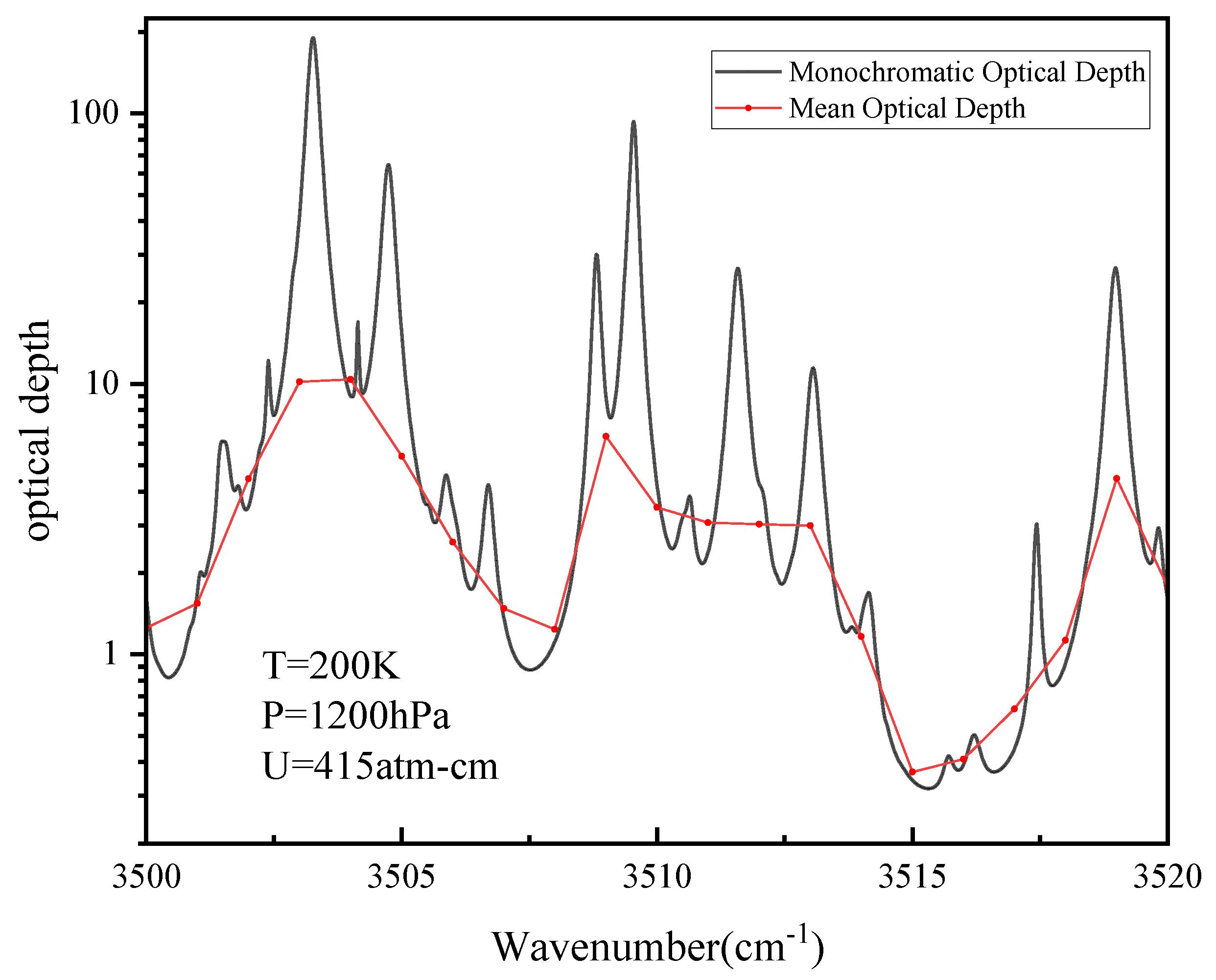
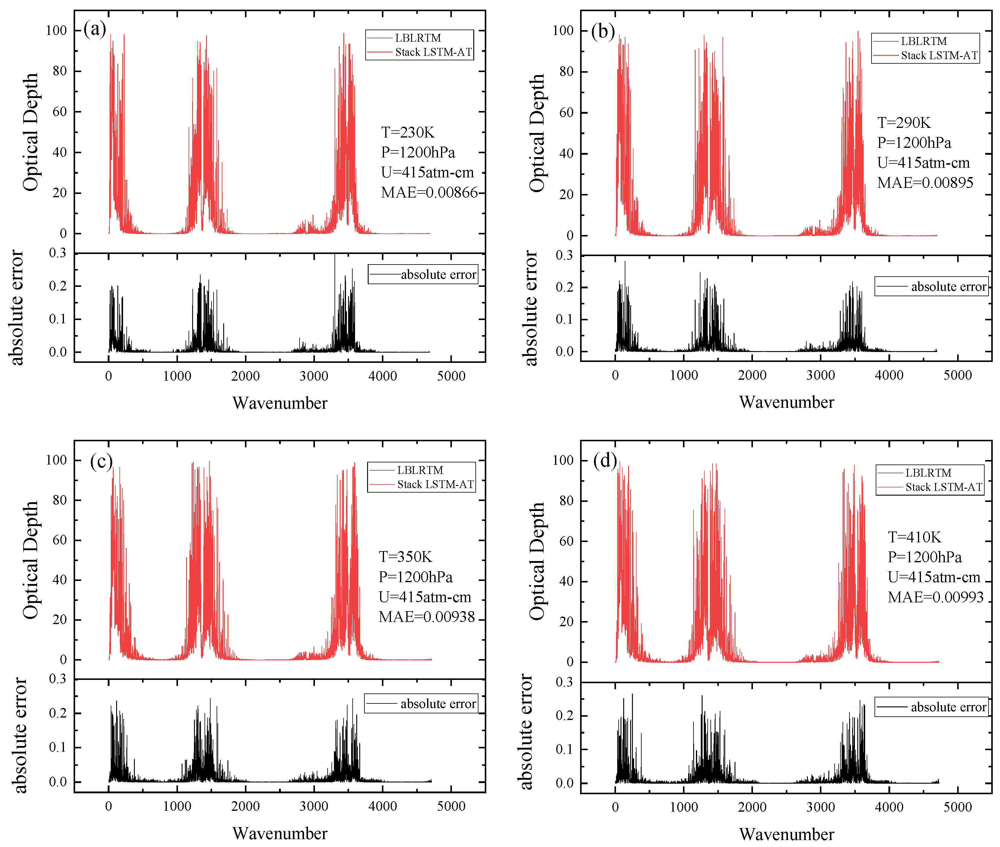
3.2.1. The Optical Depth

Figure 3a illustrates the total optical depth of water vapor under conditions where the pressure ranges from 35 to 1200 hPa, the temperature ranges from 200 to 410 K, the wavenumber ranges from 1 to 5000 cm⁻¹, and the water vapor amount is 415 atm-cm. The results show that the calculation results of LBLRTM and Stack LSTM-AT models show excellent consistency and achieve high fitting accuracy. The R² value of the fitting equation y = 0.99943x + 0.00328 is 0.9999945, indicating a strong correlation between the results of the LBLRTM and Stack LSTM-AT model. Meanwhile, the MAE and RMSE are 0.00568 and 0.02033, respectively. The minimal deviation of these error indicators further confirms the accuracy and reliability of the Stack LSTM-AT model proposed in this study. This highly consistent fitting relationship indicates that the Stack LSTM-AT model can effectively simulate the optical depth of water vapor. Figure 3b shows the scatter distribution of the absolute error in optical depth between the LBLRTM and Stack LSTM-AT model. It is evident that the absolute error is minimal in the low optical depth region; when the optical depth is less than 0.01, the absolute error remains below 0.0005. In the field of atmospheric radiative transfer and optical engineering, such an error is considered negligible. Overall, the absolute error tends to increase with the increase in optical depth, but the absolute error remains in a small range, where the maximum absolute error does not exceed 0.3. This demonstrates that the Stack LSTM-AT model can simulate the results of LBLRTM with high precision.

To test the overall accuracy and stability of the Stack LSTM-AT model, we compared the results of LBLRTM and Stack LSTM-AT under different temperatures, pressures, and water vapor amounts. Figure 4, Figure 5 and Figure 6 show the variation of optical depth with different pressures, temperatures, and water vapor amounts, respectively. We have selected multiple sets of cases with larger spans to further investigate the prediction performance. These cases involve four pressures of 35 hPa, 100 hPa, 350 hPa, and 1200 hPa, four temperatures of 230 K, 290 K, 350 K, and 410 K, and four water vapor amounts of 0.00005 atm-cm, 0.12585 atm-cm, 2.4537 atm-cm, and 415 atm-cm. The comparison of the calculation results between the LBLRTM and Stack LSTM-AT models is shown in the upper half, while the absolute error is shown in the bottom half.

Figure 4 shows the optical depth and absolute error of the LBLRTM and Stack LSTM-AT models under different pressure conditions. As illustrated in the upper part of Figure 4, three distinct absorption bands are observed within the interval of 1–5000 cm⁻¹, and the optical depth exhibits a clear trend of increasing with rising pressure overall. It is also evident that the results of the two models are in high agreement with the wavenumber, with only a slight deviation in the peak region of the strong absorption band, indicating that the proposed model can accurately simulate the optical depth at arbitrary pressure. The lower part of the figure shows the absolute errors of the two models. It is evident that the error is mainly concentrated in the three strong absorption bands. When P = 35 hPa, the maximum absolute error is no more than 0.26. With the increase in pressure, the absolute error increases slightly; when P = 1200 hPa, the maximum absolute error does not exceed 0.24. Overall, the MAE increases monotonically with increasing pressure; when P = 35 hPa, the MAE is only 0.00287, and when P = 1200 hPa, the MAE is 0.00831. It is worth noting that the results are carried out at a high-water-vapor amount of 415 atm-cm, and although local fluctuations are observed in the strong absorption spectra region, the absolute error consistently remains below 0.3, which has a negligible impact on the applications in the atmospheric radiative transfer and optical engineering. The results demonstrate that the Stack LSTM-AT model can maintain high accuracy in simulating the optical depth of water vapor over a wide pressure range.

Figure 5 shows the optical depth and absolute error of the LBLRTM and Stack LSTM-AT models under different temperature conditions. As shown in the upper part of the figures, the results of the two models are in high agreement with the wavenumber, indicating that the proposed model can accurately simulate the optical depth at arbitrary temperatures. The lower part of the figures shows the absolute errors of the two models; when T = 230 K, the maximum absolute error is no more than 0.3, and when T = 410 K, the maximum absolute error does not exceed 0.27. We must clarify that, in fact, the overall absolute errors increase slightly with the increase in temperature even though the maximum value has slightly decreased, as shown in the lower part of the figures. Overall, the distribution of absolute errors shows limited sensitivity to temperature, likely due to the pressure and water vapor amount being maintained at higher levels. In general, the MAE increases monotonically with increasing temperature. When T = 230 K, the MAE is as low as 0.00866, while when T = 410 K, it reaches 0.00993. This result validates the reliability and applicability of the Stack LSTM-AT model in a wide range of temperature conditions.

Figure 6 shows the optical depth and absolute error of the LBLRTM and Stack LSTM-AT models under different water vapor amount conditions. As shown in the upper part of the figures, the results of the two models are in high agreement with the wavenumber, indicating that the proposed model can accurately simulate the optical depth at arbitrary water vapor amount. The lower part of the figures shows the absolute errors of the two models. It is evident that the absolute error is mainly concentrated in the three strong absorption bands, with minor deviations observed in the peak region of the strong absorption band. Additionally, it is obvious that the absolute error increases with the increase in water vapor amount. When U = 0.00005 atm-cm, the maximum absolute error is no more than 4.72 × 10⁻⁵, while at U = 415 atm-cm, the maximum absolute error remains below 0.24. Overall, the MAE increases monotonically with increasing water vapor amount; when U = 0.00005 atm-cm, the MAE is 1.92246 × 10⁻⁷, and when U = 415 atm-cm, the MAE reaches 0.00831. Although the error increases slightly with a higher water vapor amount, it remains within reasonable limits. These results demonstrate that the Stack LSTM-AT model can maintain high accuracy in simulating the optical depth of water vapor over a large range of water vapor amounts.

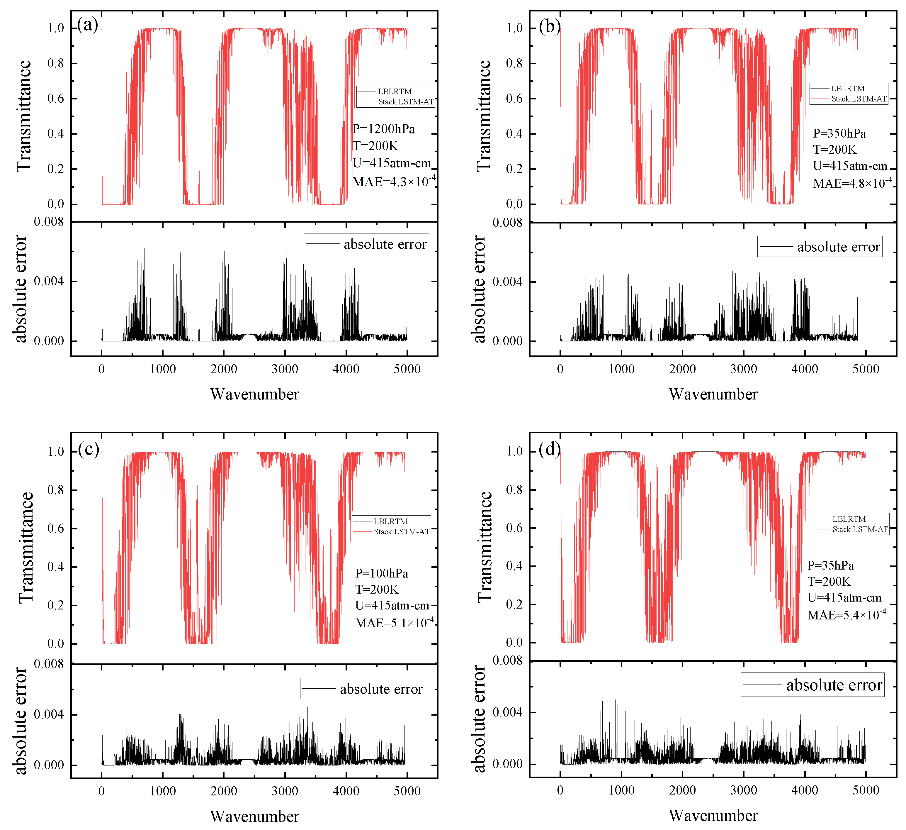
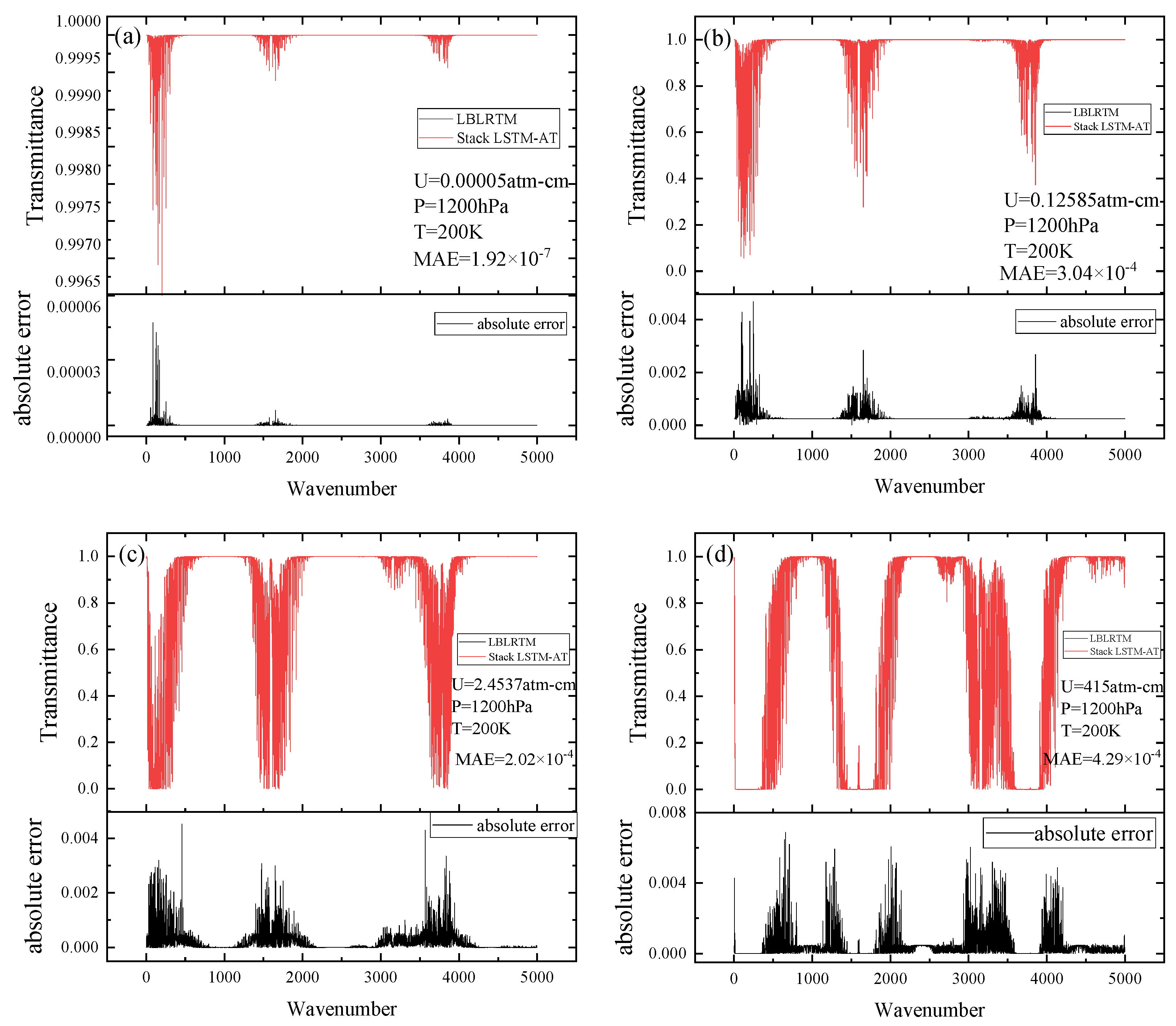
3.2.2. Atmospheric Transmittance

In this subsection, the accuracy of water vapor transmittance for the Stack LSTM-AT model is investigated under the same parameter conditions as Section 3.2.1, with comparisons made against the LBLRTM results. The overall performance, illustrated in Figure 7a, demonstrates close agreement between the two models, with no significant deviations or fluctuations; the corresponding R² value is 0.9999964, the MAE value is 5.56 × 10⁻⁴, and the RMSE value is 0.00094, respectively. Dai et al. [44] compared the MAE of the combined atmospheric radiative transfer (CART) model and MODerate resolution atmospheric TRANsmission (MODTRAN 4.0) with LBLRTM under different atmospheric conditions. The results showed that the MAE between CART and LBLRTM is 1.8 × 10⁻³, and the MAE between MODTRAN4.0 and LBLRTM is 0.0096. In comparison, the Stack LSTM-AT model achieves significantly higher accuracy. Figure 7b shows the scatter distribution of the absolute errors in atmospheric transmittance between the LBLRTM and Stack LSTM-AT model. It is evident that the absolute error increases with the increase in transmittance. In the low transmittance region, the absolute errors are smaller and more concentrated, while in the high transmittance region, the dispersion of the absolute errors increases slightly. Notably, despite these variations, all absolute errors maintain a consistently small order of magnitude across the entire transmittance region. This consistent performance, particularly the maintenance of errors within acceptable limits throughout different transmittance conditions, strongly indicates the model’s robust stability and reliability.

To further investigate the predictive performance of the Stack LSTM-AT model under complex environmental conditions, it is necessary to systematically evaluate the predictive accuracy of the Stack LSTM-AT model at different temperatures, pressures, and water vapor amounts. Figure 8, Figure 9 and Figure 10 analyzed the independent effects of various parameters on the prediction accuracy of the Stack LSTM-AT model while examining the stability of the Stack LSTM-AT model under extreme conditions by setting reasonable parameters.

Figure 8 shows the atmospheric transmittance and absolute error of the LBLRTM and Stack LSTM-AT model under different pressure conditions. As shown in the upper part of the figures, the results of the two models are in high agreement with the wavenumber, indicating that the proposed model can accurately simulate the atmospheric transmittance at arbitrary pressure. The lower part of the figures shows the absolute errors of the two models. It is evident that the error is mainly concentrated in the three strong absorption bands. When P = 35 hPa, the maximum absolute error is no more than 0.005, and at P = 1200 hPa, the maximum absolute error does not exceed 0.007. Overall, the MAE increases monotonically with decreasing pressure, while when P = 1200 hPa, the MAE is 4.3 × 10⁻⁴, and when P = 35 hPa, the MAE is 5.4 × 10⁻⁴. Cui et al. [45] developed a fast computational method based on the BPNN model. The MAE and R² between the BPNN model and LBLRTM are 6.08 × 10⁻⁴ and 0.9996, respectively. However, the maximum absolute error between the BPNN model and LBLRTM is about 0.07. Therefore, the Stack LSTM-AT model in this study demonstrates better accuracy and stability. These results demonstrate that the Stack LSTM-AT model can maintain high accuracy in simulating the atmospheric transmittance of water vapor over a large pressure range.

Figure 9 shows the atmospheric transmittance and absolute error of the LBLRTM and Stack LSTM-AT models under different temperature conditions. As shown in the upper part of the figures, the results of the two models are in high agreement with the wavenumber, indicating that the proposed model can accurately simulate the atmospheric transmittance at arbitrary temperature. The lower part of the figures shows the absolute errors of the two models; when T = 230 K, the maximum absolute error is no more than 0.0068, and when T = 410 K, the maximum absolute error does not exceed 0.007. Overall, when P = 1200 hPa, the MAE is 0.00831, and when P = 35 hPa, the MAE is only 0.00287. This result indicates that the Stack LSTM-AT model can maintain high accuracy in simulating the atmospheric transmittance of water vapor over a large temperature range.

Figure 10 shows the atmospheric transmittance and absolute error of the LBLRTM and Stack LSTM-AT models under different water vapor amount conditions. As shown in the upper part of the figures, the results of the two models are in high agreement with the wavenumber, indicating that the proposed model can accurately simulate the atmospheric transmittance at arbitrary water vapor amount. The lower part of the figures shows the absolute errors of the two models. It is obvious that the absolute error increases with the increase in water vapor amount. When U = 0.00005 atm-cm, the maximum absolute error is no more than 4.7 × 10⁻⁵, while at U = 415 atm-cm, the maximum absolute error remains below 0.00687. Overall, when U = 0.00005 atm-cm, the MAE is 1.92 × 10⁻⁷; with the increase in water vapor amount, the absolute errors increase slightly, and when U = 415 atm-cm, the MAE reaches 4.29 × 10⁻⁴, which is still within the acceptable range. Wei et al. [39] compared the absolute error of FFTM with LBLRTM, and the results showed that the maximum absolute error between CART and LBLRTM is 0.008, which is larger than our model. This result indicates that the Stack LSTM-AT model can maintain high accuracy in simulating the atmospheric transmittance over a large water vapor amount range.

3.2.3. Calculation Time

To evaluate the computational efficiency of several models, we conducted five independent experiments and averaged the computational times. The results are shown in

Table 3. Comparison of computing time among three models.

Model	Time (s)
Single LSTM	3.567 × 10−2
Stack LSTM	8.755 × 10−2
Self-attention	4.91 × 10−2
LSTM-AT	7.764 × 10−2
Stack LSTM-AT	9.784 × 10−2
LBLRTM	284.943

. The experimental environment was built on an Intel Core i5-13490F CPU, equipped with 8 GB of RAM, and run on the Windows 10 64-bit operating system.

The results show that the Stack LSTM-AT model computes a single spectrum (1–5000 cm⁻¹) in 9.784 × 10⁻² s. This computational speed is impressive, especially since it covers such a wide range of wavenumbers. Although our model is not as fast as the other models, its computational time is drastically reduced compared to the conventional LBLRTM model. This clearly shows that the model proposed in this paper significantly improves the computational efficiency, and the computational speed is increased by thousands of times [46]. This clearly demonstrates that the model proposed in this paper has achieved a substantial improvement in computational efficiency, with a speedup of several thousand times.

Importantly, our model balances accuracy and speed effectively. While training the model takes more time initially, once trained, it can perform calculations very quickly. This significantly saves computing resources and time in real-world applications. In conclusion, the Stack LSTM-AT model presented in this paper significantly enhances computational efficiency compared to traditional methods, providing a highly efficient and reliable solution for large-scale data computation.

4. Conclusions

Accurate and efficient calculation of water vapor atmospheric transmittance is of paramount importance in various scientific and engineering fields, including radiative transfer, remote sensing, and optoelectronic engineering applications. While existing computational methods have made significant progress, they remain constrained by various limitations, leaving substantial room for algorithmic improvements. In this study, we developed an advanced deep learning architecture, the Stack LSTM-AT Model, which integrates LSTM with a self-attention mechanism. The predicted results for optical depth and atmospheric transmittance are compared to the results of LBLRTM. The results show that the Stack LSTM-AT model achieves remarkable accuracy and robustness. The absolute errors were consistently below 0.3 in optical depth and 0.01 in transmittance throughout all experimental conditions. Overall, the MAE, RMSE, and R² of the optical depth reached about 0.00568, 0.02033, and 0.9999945, respectively, while the MAE, RMSE, and R² of the atmospheric transmittance reached about 5.5586 × 10⁻⁴, 0.00094, and 0.9999964, respectively. Additionally, in terms of efficiency, the computational time of the Stack LSTM-AT model is 9.784 × 10⁻² s. This is thousands of times more efficient compared to LBLRTM. The Stack LSTM-AT model shows high prediction accuracy while improving operational efficiency, which provides an efficient and high-precision solution for rapid estimation of the water vapor transmission rate and other radiation parameters.

It should be noted that although the Stack LSTM-AT model can quickly calculate atmospheric transmittance under most homogeneous atmospheric conditions, the actual atmospheric conditions are often very complex and non-homogeneous. Although traditional methods such as the Curtis-Godson (CG) approximation and the correlated k-distribution (CKD) can partially adapt to non-homogeneous atmospheric conditions, their applicability remains limited, and the prediction accuracy of the model is difficult to guarantee. Therefore, we aim to develop more advanced deep learning architectures to achieve higher accuracy in handling complex atmospheric environments, providing a more reliable solution for transmittance calculations in non-homogeneous paths. Hence, future research will focus on optimizing model architectures to further improve transmittance prediction accuracy and generalization capability. For example, the t-distributed Stochastic Neighbor Embedding (t-SNE) method may be employed to project complex inhomogeneous atmospheric parameters into low-dimensional spaces while preserving local data structures, thereby simplifying model architecture and reducing computational complexity. Additionally, Transformer’s robust long-range dependency modeling capability may be useful to effectively process layered atmospheric layered data with non-local interactions. Finally, we hope to integrate these optimized models into the self-developed CART. This integration will improve the software’s accuracy in predicting atmospheric transmittance and significantly increase its computational efficiency, making it a more powerful tool for researchers and practitioners in the field. The enhanced version of CART will be able to handle a wide range of atmospheric conditions from homogeneous to highly non-homogeneous paths while maintaining a user-friendly interface and seamless compatibility with existing atmospheric datasets.

It is hoped that this study can provide new insights and methods for development in the field of atmospheric radiative transfer and remote sensing applications and make meaningful contributions to related research areas.

References

1. Soden, B.J.; Held, I.M. An Assessment of Climate Feedbacks in Coupled Ocean–Atmosphere Models. J. Clim. 2006, 19, 3354–3360. [Google Scholar]
2. Chen, Y.; Han, Y.; Van Delst, P.; Weng, F. On Water Vapor Jacobian in Fast Radiative Transfer Model. J. Geophys. Res. Atmospheres 2010, 115. [Google Scholar]
3. Schneider, T.; O’Gorman, P.A.; Levine, X.J. Water Vapor and the Dynamics of Climate Changes. Rev. Geophys. 2010, 48. [Google Scholar]
4. Colman, R. A Comparison of Climate Feedbacks in General Circulation Models. Clim. Dyn. 2003, 20, 865–873. [Google Scholar]
5. Vaquero-Martínez, J.; Antón, M.; de Galisteo, J.P.O.; Román, R.; Cachorro, V.E. Water Vapor Radiative Effects on Short-Wave Radiation in Spain. Atmos. Res. 2018, 205, 18–25. [Google Scholar]
6. Clough, S.A.; Iacono, M.J.; Moncet, J. Line-by-Line Calculations of Atmospheric Fluxes and Cooling Rates: Application to Water Vapor. J. Geophys. Res. Atmos. 1992, 97, 15761–15785. [Google Scholar]
7. Clough, S.; Shephard, M.; Mlawer, E.; Delamere, J.; Iacono, M.; Cady-Pereira, K.; Boukabara, S.; Brown, P. Atmospheric Radiative Transfer Modeling: A Summary of the Aer Codes. J. Quant. Spectrosc. Radiat. Transf. 2005, 91, 233–244. [Google Scholar]
8. Li, W.; Zhang, F.; Shi, Y.-N.; Iwabuchi, H.; Zhu, M.; Li, J.; Han, W.; Letu, H.; Ishimoto, H. Efficient Radiative Transfer Model for Thermal Infrared Brightness Temperature Simulation in Cloudy Atmospheres. Opt. Express 2020, 28, 25730–25749. [Google Scholar]
9. Morcrette, J.-J.; Mozdzynski, G.; Leutbecher, M. A Reduced Radiation Grid for the Ecmwf Integrated Forecasting System. Mon. Weather Rev. 2008, 136, 4760–4772. [Google Scholar]
10. Manners, J.; Thelen, J.C.; Petch, J.; Hill, P.; Edwards, J.M. Two Fast Radiative Transfer Methods to Improve the Temporal Sampling of Clouds in Numerical Weather Prediction and Climate Models. Q. J. R. Meteorol. Soc. J. Atmos. Sci. Appl. Meteorol. Phys. Oceanogr. 2009, 135, 457–468. [Google Scholar]
11. Isaacs, R.G.; Vogelmann, A.M. Multispectral Sensor Data Simulation Modeling Based on the Multiple Scattering Lowtran Code. Remote Sens. Environ. 1988, 26, 75–99. [Google Scholar]
12. Berk, A.; Bernstein, L.S.; Anderson, G.P.; Acharya, P.; Robertson, D.; Chetwynd, J.; Adler-Golden, S. Modtran Cloud and Multiple Scattering Upgrades with Application to Aviris. Remote Sens. Environ. 1998, 65, 367–375. [Google Scholar]
13. Strow, L.L.; Hannon, S.E.; De-Souza Machado, S.; Motteler, H.E.; Tobin, D.C. Validation of the Atmospheric Infrared Sounder Radiative Transfer Algorithm. J. Geophys. Res. Atmos. 2006, 111. [Google Scholar]
14. Engelen, R.J.; Stephens, G.L. Infrared Radiative Transfer in the 9.6-Μm Band: Application to TIROS Operational Vertical Sounder Ozone Retrieval. J. Geophys. Res. Atmos. 1997, 102, 6929–6939. [Google Scholar] [CrossRef]
15. Buchwitz, M.; Rozanov, V.V.; Burrows, J.P. A Correlated-K Distribution Scheme for Overlapping Gases Suitable for Retrieval of Atmospheric Constituents from Moderate Resolution Radiance Measurements in the Visible/near-Infrared Spectral Region. J. Geophys. Res. Atmos. 2000, 105, 15247–15261. [Google Scholar]
16. Stegmann, P.G.; Johnson, B.; Moradi, I.; Karpowicz, B.; McCarty, W. A Deep Learning Approach to Fast Radiative Transfer. J. Quant. Spectrosc. Radiat. Transf. 2022, 280, 108088. [Google Scholar]
17. Cotronei, A.; Slawig, T. Single-Precision Arithmetic in ECHAM Radiation Reduces Runtime and Energy Consumption. Geosci. Model Dev. 2020, 13, 2783–2804. [Google Scholar]
18. Alizamir, M.; Shiri, J.; Fard, A.F.; Kim, S.; Gorgij, A.D.; Heddam, S.; Singh, V.P. Improving the Accuracy of Daily Solar Radiation Prediction by Climatic Data Using an Efficient Hybrid Deep Learning Model: Long Short-Term Memory (LSTM) Network Coupled with Wavelet Transform. Eng. Appl. Artif. Intell. 2023, 123, 106199. [Google Scholar] [CrossRef]
19. Lu, Y.; Wang, L.; Zhu, C.; Zou, L.; Zhang, M.; Feng, L.; Cao, Q. Predicting Surface Solar Radiation Using a Hybrid Radiative Transfer–Machine Learning Model. Renew. Sustain. Energy Rev. 2023, 173, 113105. [Google Scholar]
20. André, F.; Cornet, C.; Delage, C.; Dubuisson, P.; Galtier, M. On the Use of Recurrent Neural Networks for Fast and Accurate Non-Uniform Gas Radiation Modeling. J. Quant. Spectrosc. Radiat. Transf. 2022, 293, 108371. [Google Scholar] [CrossRef]
21. Chevallier, F.; Chéruy, F.; Scott, N.A.; Chédin, A. A Neural Network Approach for a Fast and Accurate Computation of a Longwave Radiative Budget. J. Appl. Meteorol. 1998, 37, 1385–1397. [Google Scholar] [CrossRef]
22. Krasnopolsky, V.M.; Fox-Rabinovitz, M.S.; Belochitski, A.A. Decadal Climate Simulations Using Accurate and Fast Neural Network Emulation of Full, Longwave and Shortwave, Radiation. Mon. Weather Rev. 2008, 136, 3683–3695. [Google Scholar]
23. Hochreiter, S.; Schmidhuber, J. Long Short-Term Memory. Neural Comput. 1997, 9, 1735–1780. [Google Scholar] [PubMed]
24. Greff, K.; Srivastava, R.K.; Koutník, J.; Steunebrink, B.R.; Schmidhuber, J. LSTM: A Search Space Odyssey. IEEE Trans. Neural Netw. Learn. Syst. 2017, 28, 2222–2232. [Google Scholar] [PubMed]
25. Demir, F. Deepcoronet: A Deep LSTM Approach for Automated Detection of COVID-19 Cases from Chest X-Ray Images. Appl. Soft Comput. 2021, 103, 107160. [Google Scholar] [PubMed]
26. Mamdouh, M.; Ezzat, M.; Hefny, H. Improving Flight Delays Prediction by Developing Attention-Based Bidirectional LSTM Network. Expert Syst. Appl. 2024, 238, 121747. [Google Scholar]
27. Huang, F.; Li, X.; Yuan, C.; Zhang, S.; Zhang, J.; Qiao, S. Attention-Emotion-Enhanced Convolutional LSTM for Sentiment Analysis. IEEE Trans. Neural Netw. Learn. Syst. 2022, 33, 4332–4345. [Google Scholar]
28. Chen, Y.; Rao, M.; Feng, K.; Zuo, M.J. Physics-Informed LSTM Hyperparameters Selection for Gearbox Fault Detection. Mech. Syst. Signal Process. 2022, 171, 108907. [Google Scholar] [CrossRef]
29. Wang, Z.; Zhang, Y.; Li, G.; Zhang, J.; Zhou, H.; Wu, J. A Novel Solar Irradiance Forecasting Method Based on Multi-Physical Process of Atmosphere Optics and LSTM-Bp Model. Renew. Energy 2024, 226, 120367. [Google Scholar]
30. Zhao, X.; Niu, Q.; Chi, Q.; Chen, J.; Liu, C. A New LSTM-Based Model to Determine the Atmospheric Weighted Mean Temperature in Gnss Pwv Retrieval. GPS Solut. 2024, 28, 74. [Google Scholar] [CrossRef]
31. Li, Y.; Zhu, Z.; Kong, D.; Han, H.; Zhao, Y. Ea-LSTM: Evolutionary Attention-Based LSTM for Time Series Prediction. Knowl. Based Syst. 2019, 181, 104785. [Google Scholar] [CrossRef]
32. Cai, S.; Gao, H.; Zhang, J.; Peng, M. A Self-Attention-LSTM Method for Dam Deformation Prediction Based on Ceemdan Optimization. Appl. Soft Comput. 2024, 159, 111615. [Google Scholar] [CrossRef]
33. Liu, L.; Xu, X. Self-Attention Mechanism at the Token Level: Gradient Analysis and Algorithm Optimization. Knowl.-Based Syst. 2023, 277, 110784. [Google Scholar]
34. Xie, Y.; Liang, R.; Liang, Z.; Huang, C.; Zou, C.; Schuller, B. Speech Emotion Classification Using Attention-Based LSTM. IEEE/ACM Trans. Audio Speech Lang. Process. 2019, 27, 1675–1685. [Google Scholar] [CrossRef]
35. Pan, S.; Yang, B.; Wang, S.; Guo, Z.; Wang, L.; Liu, J.; Wu, S. Oil Well Production Prediction Based on Cnn-LSTM Model with Self-Attention Mechanism. Energy 2023, 284, 128701. [Google Scholar]
36. Zang, H.; Xu, R.; Cheng, L.; Ding, T.; Liu, L.; Wei, Z.; Sun, G. Residential Load Forecasting Based on LSTM Fusing Self-Attention Mechanism with Pooling. Energy 2021, 229, 120682. [Google Scholar]
37. Xia, J.; Feng, Y.; Lu, C.; Fei, C.; Xue, X. LSTM-Based Multi-Layer Self-Attention Method for Remaining Useful Life Estimation of Mechanical Systems. Eng. Fail. Anal. 2021, 125, 105385. [Google Scholar]
38. Rothman, L.S. History of the Hitran Database. Nat. Rev. Phys. 2021, 3, 302–304. [Google Scholar] [CrossRef]
39. Wei, H.; Chen, X.; Rao, R.; Wang, Y.; Yang, P. A Moderate-Spectral-Resolution Transmittance Model Based on Fitting the Line-by-Line Calculation. Opt. Express 2007, 15, 8360–8370. [Google Scholar]
40. Turkoglu, M.O.; D’Aronco, S.; Wegner, J.D.; Schindler, K. Gating Revisited: Deep Multi-Layer RNNs That Can Be Trained. IEEE Trans. Pattern Anal. Mach. Intell. 2022, 44, 4081–4092. [Google Scholar]
41. Guo, P.; Wang, P. Qhan: Quantum-Inspired Hierarchical Attention Mechanism Network for Question Answering. Int. J. Artif. Intell. Tools 2023, 32, 2360009. [Google Scholar]
42. Niu, Z.; Zhong, G.; Yu, H. A Review on the Attention Mechanism of Deep Learning. Neurocomputing 2021, 452, 48–62. [Google Scholar] [CrossRef]
43. Gülmez, B. Stock Price Prediction with Optimized Deep LSTM Network with Artificial Rabbits Optimization Algorithm. Expert Syst. Appl. 2023, 227, 120346. [Google Scholar] [CrossRef]
44. Dai, C.; Wei, H.; Chen, X. Validation of the Precision of Atmospheric Molecular Absorption and Thermal Radiance Calculated by Combined Atmospheric Radiative Transfer(C 10 Art) Code. Infrared Laser Eng. 2013, 42, 174–180. [Google Scholar]
45. Cui, J.; Zhang, J.; Dong, C.; Liu, D.; Huang, X. An Ultrafast and High Accuracy Calculation Method for Gas Radiation Characteristics Using Artificial Neural Network. Infrared Phys. Technol. 2020, 108, 103347. [Google Scholar]
46. Zhou, J.; Dai, C.; Wu, P.; Wei, H. A Fast Computing Model for the Oxygen a-Band High-Spectral-Resolution Absorption Spectra Based on Artificial Neural Networks. Remote Sens. 2024, 16, 3616. [Google Scholar] [CrossRef]
Figure 1. Architecture of the proposed model. (1) The four main modules comprising Stack LSTM-AT. (2) LSTM network architecture. (3) Self-attention mechanism.
Remotesensing 17 01224 g001
Figure 2. The mean optical depth averaged with a spectral resolution of 1 cm−1 and the monochromatic optical depth for water vapor at T = 200 K, P = 1200 hPa, and U = 415 atm-cm.
Remotesensing 17 01224 g002
Figure 3. Comparison of optical depth between LBLRTM and Stack LSTM-AT. (a) Comparison of optical depth between LBLRTM and Stack LSTM-AT. (b) Absolute error of optical depth between LBLRTM and Stack LSTM-AT.
Remotesensing 17 01224 g003
Figure 4. The optical depth varies with pressure under the conditions of a temperature of 200 K and a water vapor amount of 415 atm-cm. (a) 1200 hPa. (b) 350 hPa. (c) 100 hPa. (d) 35 hPa.
Remotesensing 17 01224 g004
Figure 5. The optical depth varies with temperature under the conditions of a pressure of 1200 hPa and a water vapor amount of 415 atm-cm. (a) 200 K. (b) 290 K. (c) 350 K. (d) 410 K.
Remotesensing 17 01224 g005
Figure 6. The optical depth varies with water vapor amount under the conditions of a temperature of 200 K and a pressure of 1200 hPa. (a) 0.00005 atm-cm. (b) 0.12585 atm-cm. (c) 2.4537 atm-cm. (d) 415 atm-cm.
Remotesensing 17 01224 g006
Figure 7. Comparison of atmospheric transmittance between LBLRTM and Stack LSTM-AT. (a) Comparison of atmospheric transmittance between LBLRTM and Stack LSTM-AT. (b) Absolute error of atmospheric transmittance.
Remotesensing 17 01224 g007
Figure 8. The atmospheric transmittance varies with pressure under the conditions of a temperature of 200 K and a water vapor amount of 415 atm-cm. (a) 1200 hPa. (b) 350 hPa. (c) 100 hPa. (d) 35 hPa.
Remotesensing 17 01224 g008
Figure 9. The atmospheric transmittance varies with temperature under the conditions of a pressure of 1200 hPa and a water vapor amount of 415 atm-cm. (a) 200 K. (b) 290 K. (c) 350 K. (d) 410 K.
Remotesensing 17 01224 g009
Figure 10. The atmospheric transmittance varies with water vapor amount under the conditions of a temperature of 200 K and a pressure of 1200 hPa. (a) 0.00005 atm-cm. (b) 0.12585 atm-cm. (c) 2.4537 atm-cm. (d) 415 atm-cm.
Remotesensing 17 01224 g010