
Domain Adaptation and Fine-Tuning of a Deep Learning Segmentation Model of Small Agricultural Burn Area Detection Using High-Resolution Sentinel-2 Observations: A Case Study of Punjab, India


Abstract

1. Introduction
2. Related Work
3. Data and Method
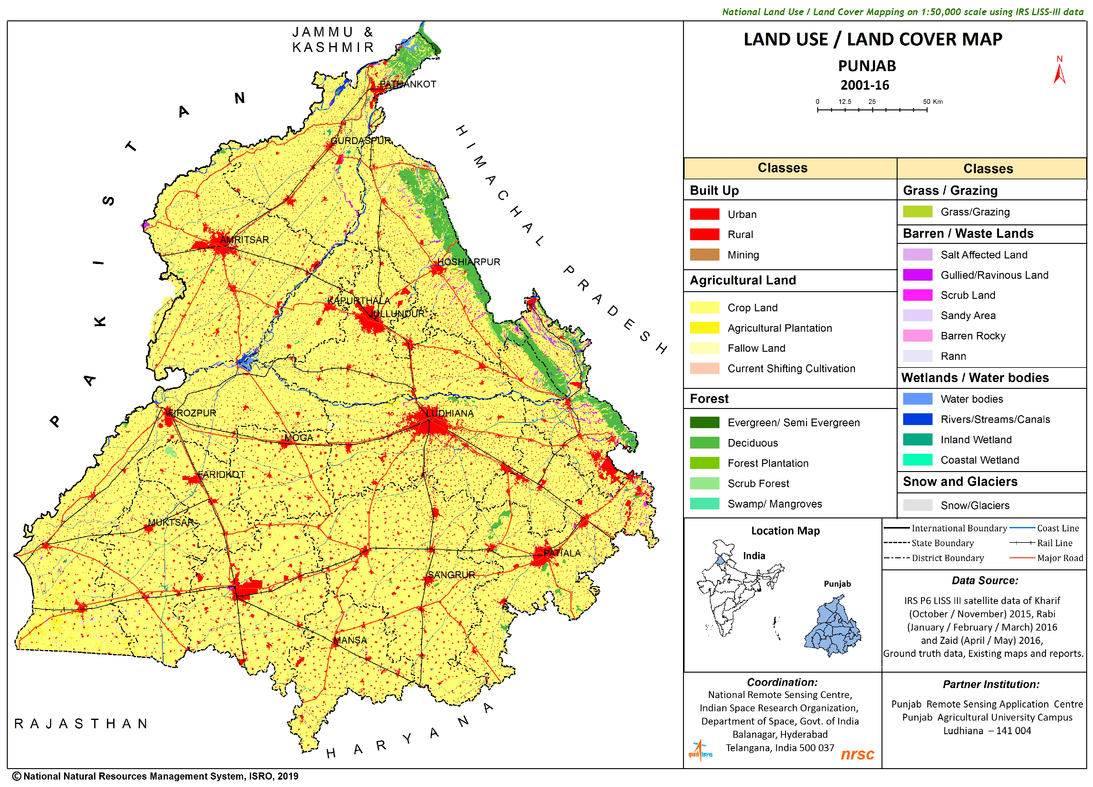
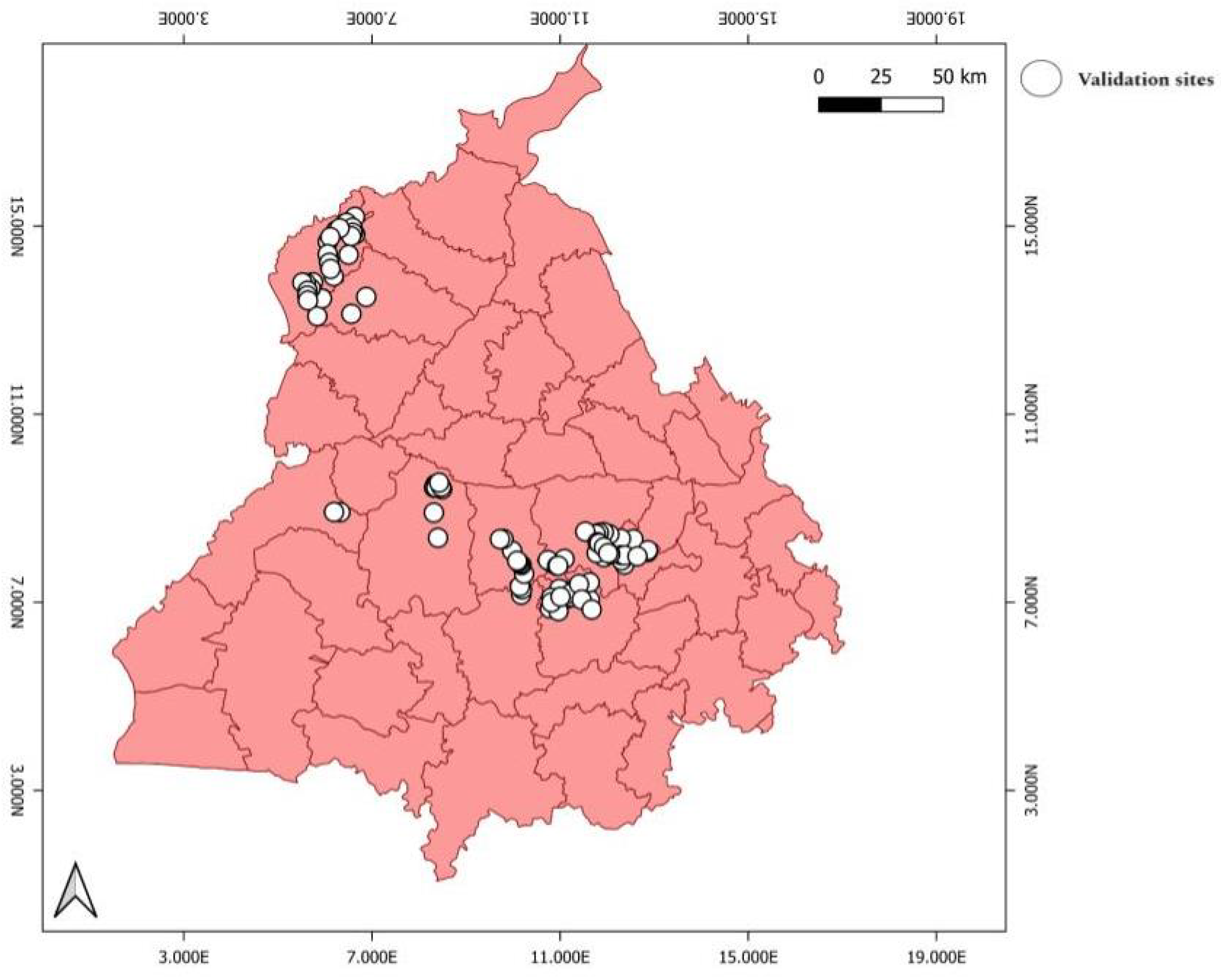
3.1. Study Area
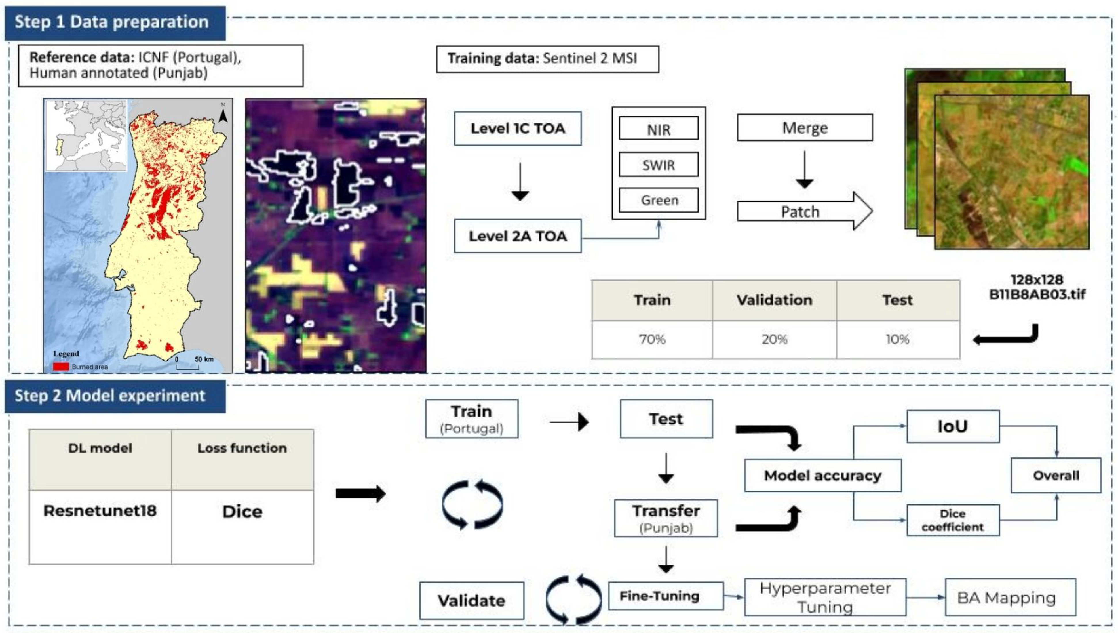
3.2. Data Acquisition and Atmospheric Correction
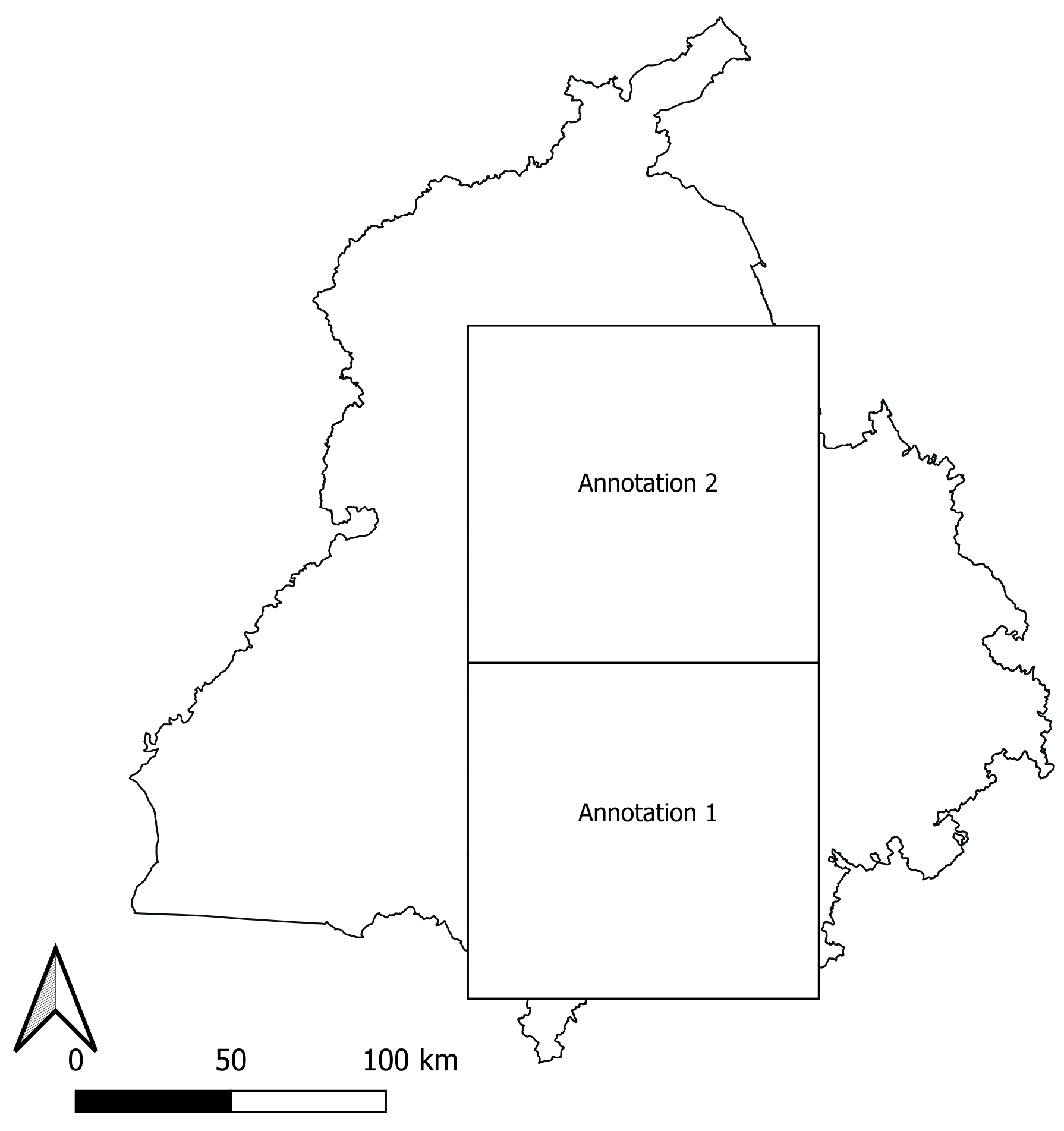
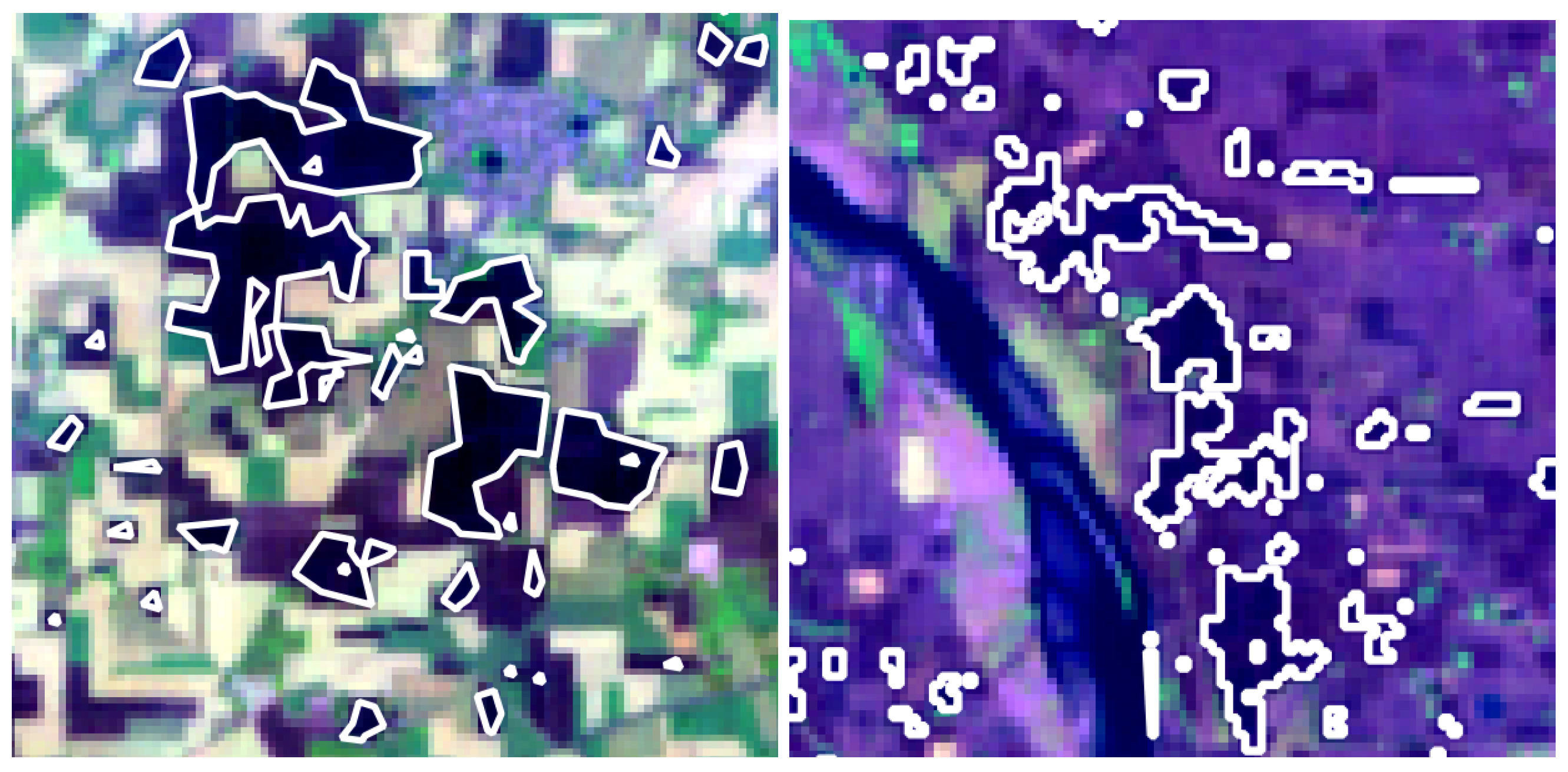
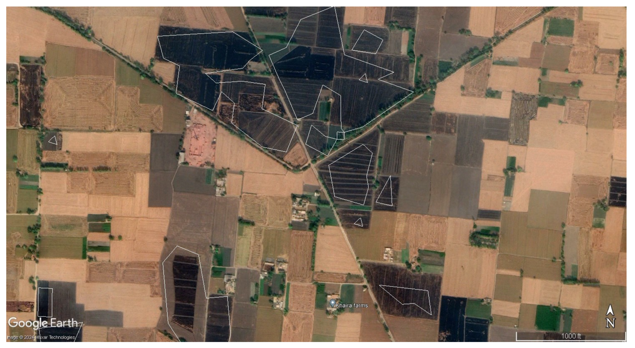
3.3. Preparation of Reference Data
3.4. Data Pipeline
3.5. Baseline Model
3.6. Model Framework
Hyperparameter Setting
3.7. Experiment Setup
3.7.1. Evaluation Metrics
4. Results
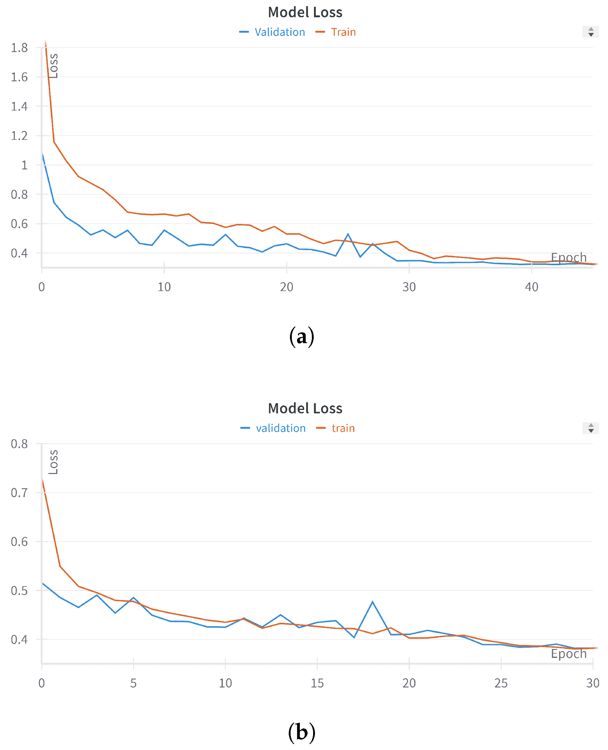
Model Performance
5. Discussion
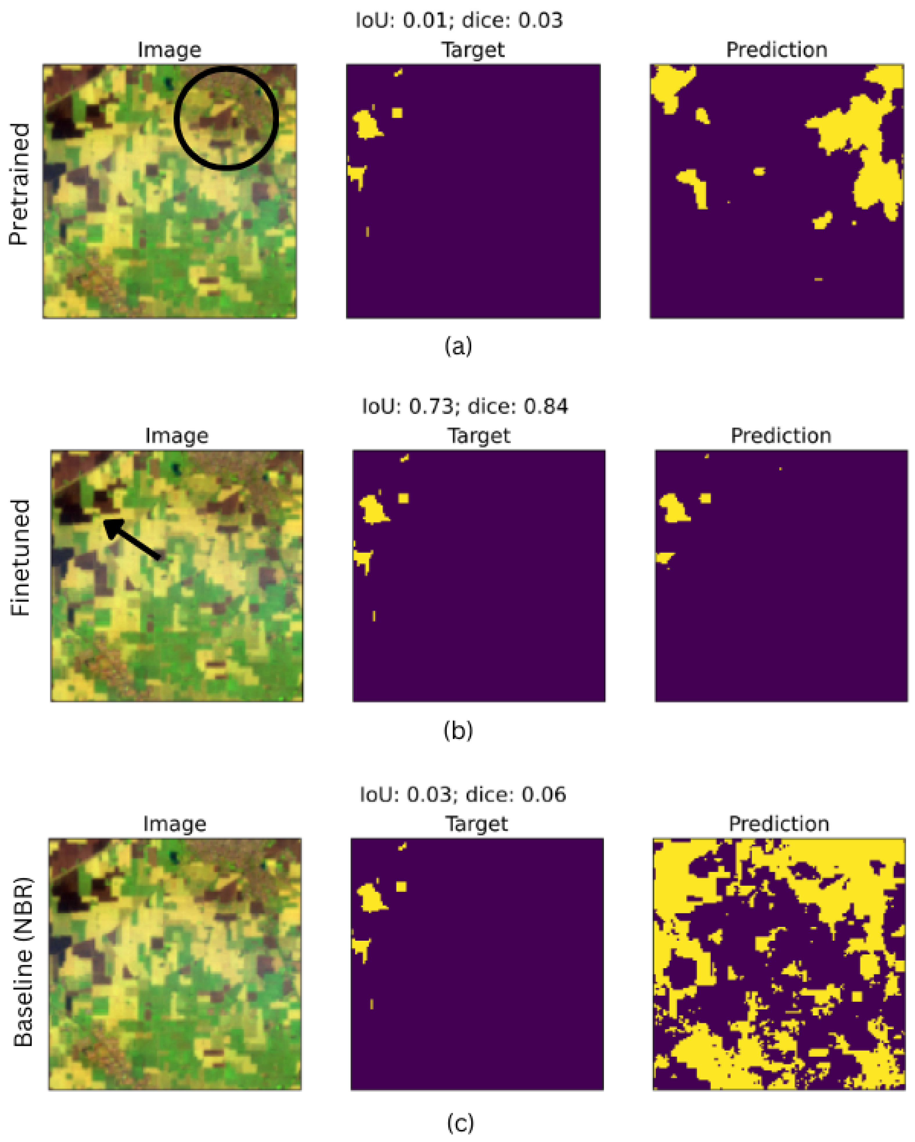
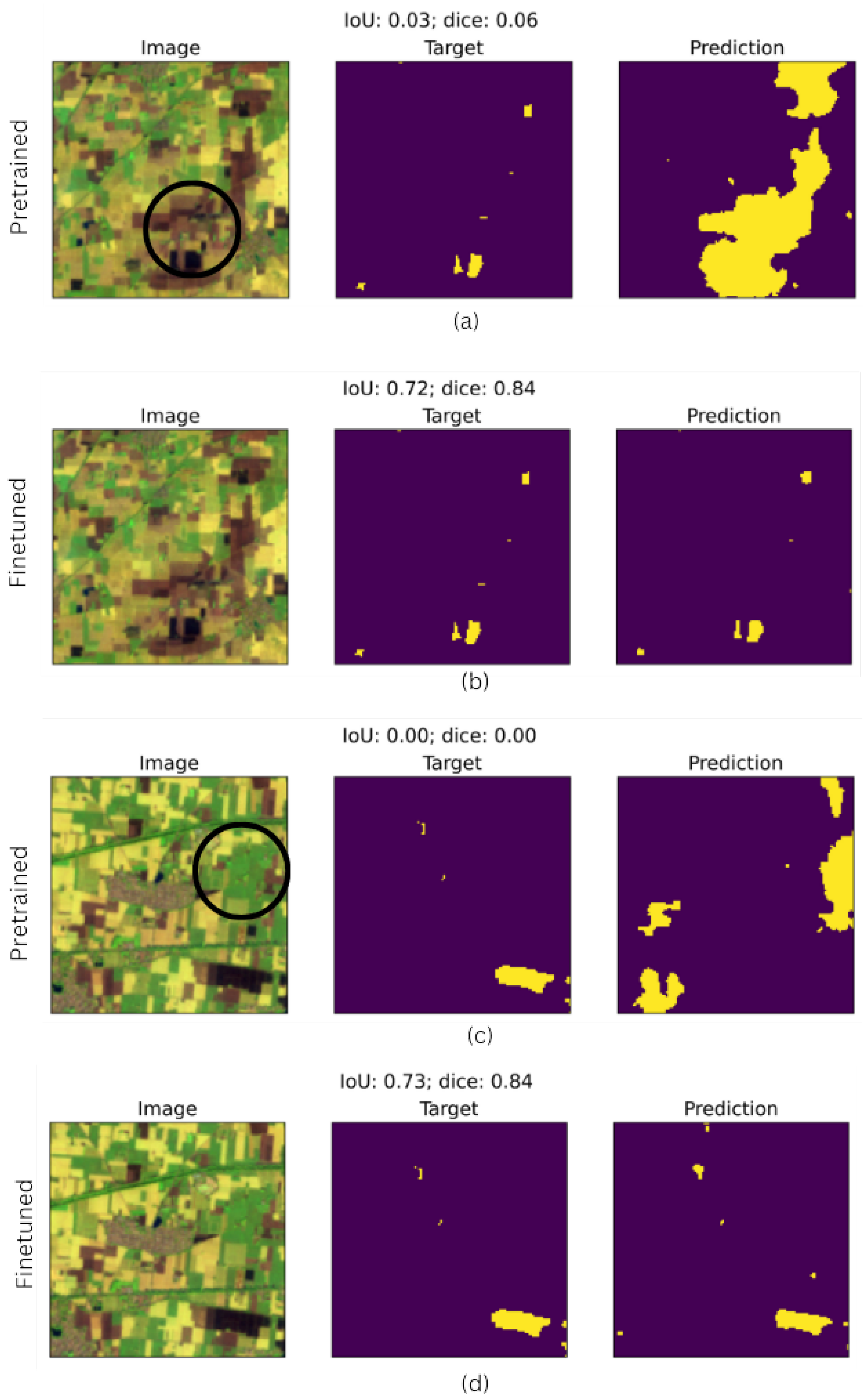
5.1. Pre-Tuned vs. Fine-Tuned Model Performanc
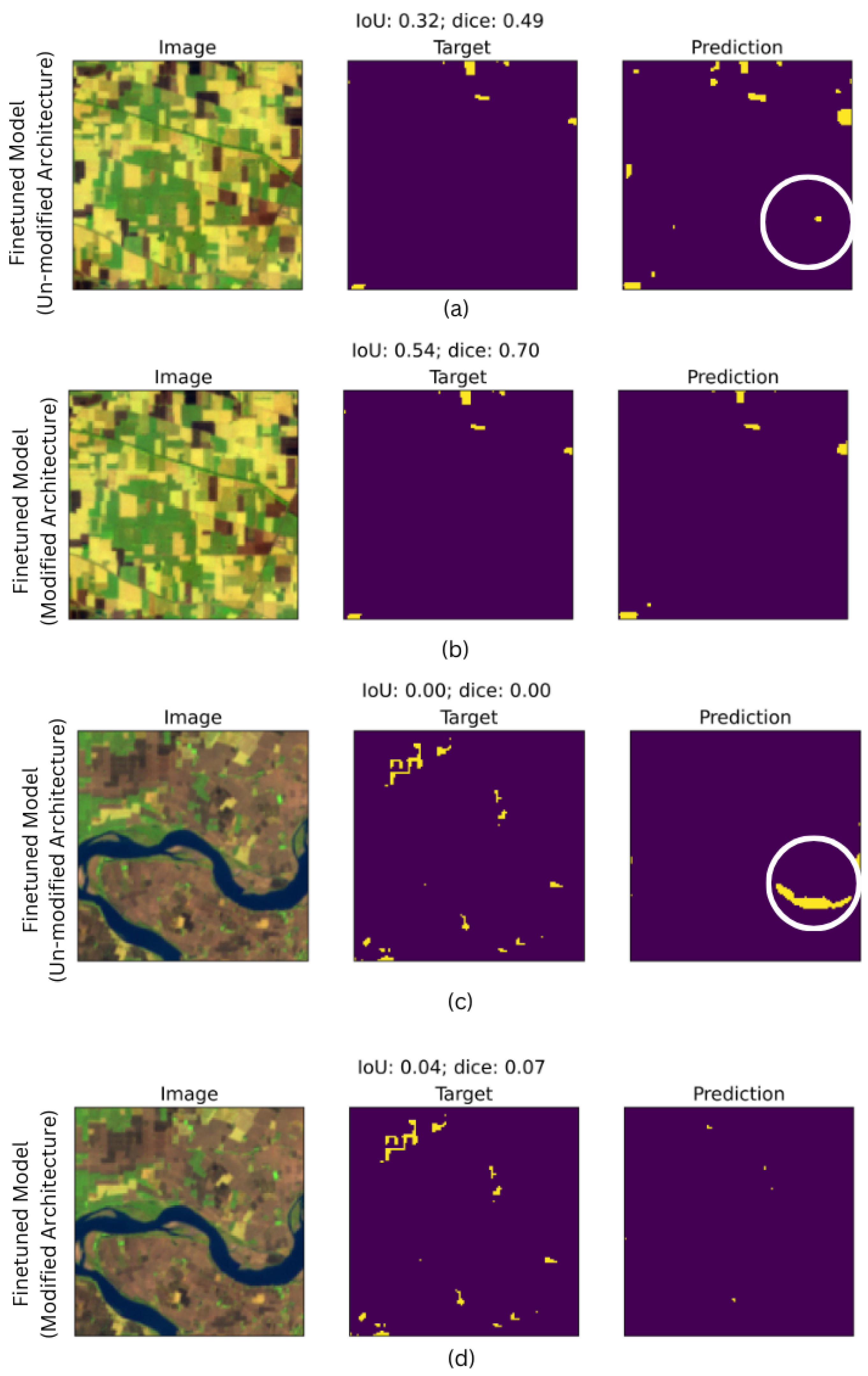
5.1.1. Impact of Architectural Modification and Annotation Data on Segmentation Task
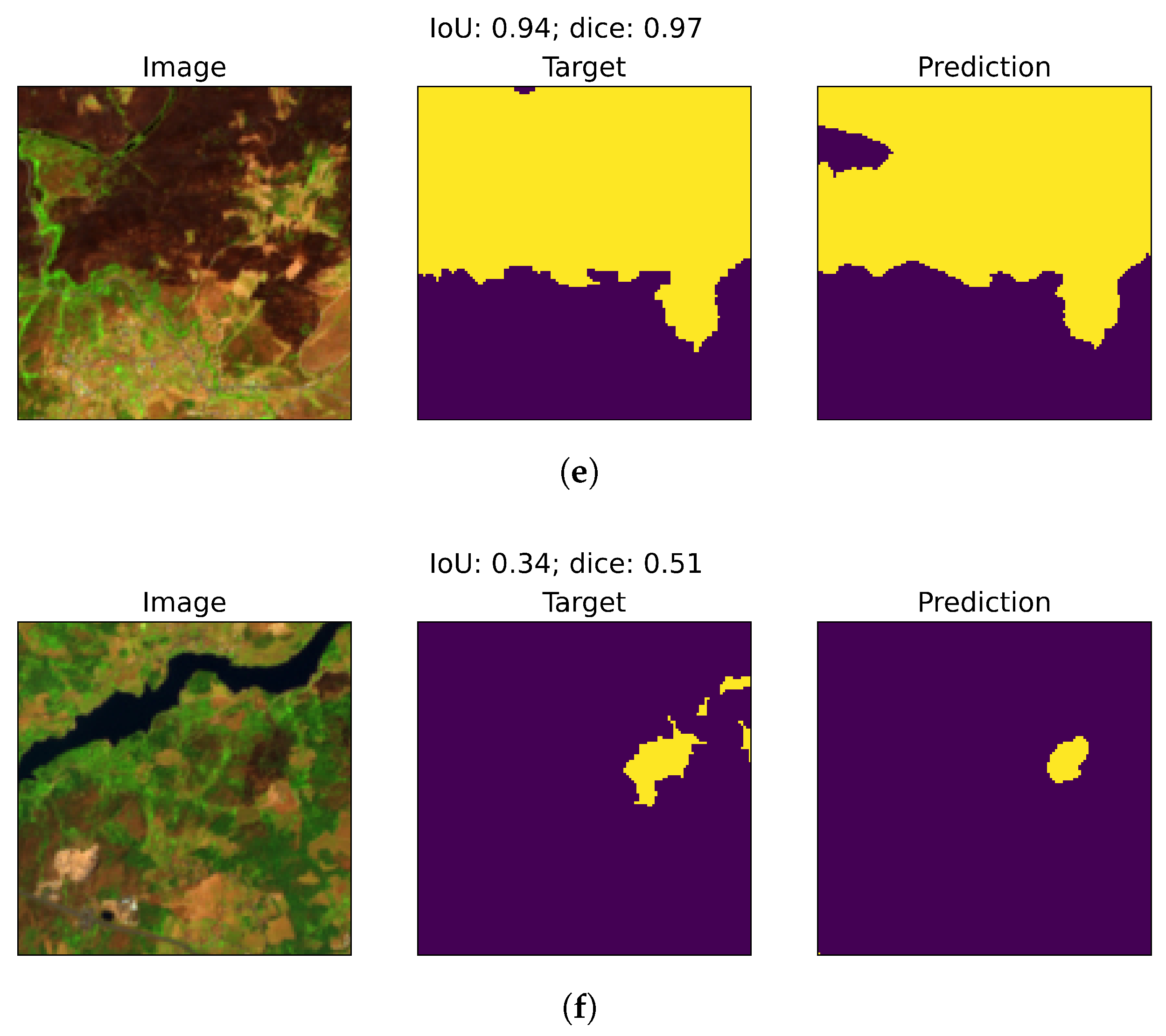
5.1.2. Model Sensitivity over Small Burn Area
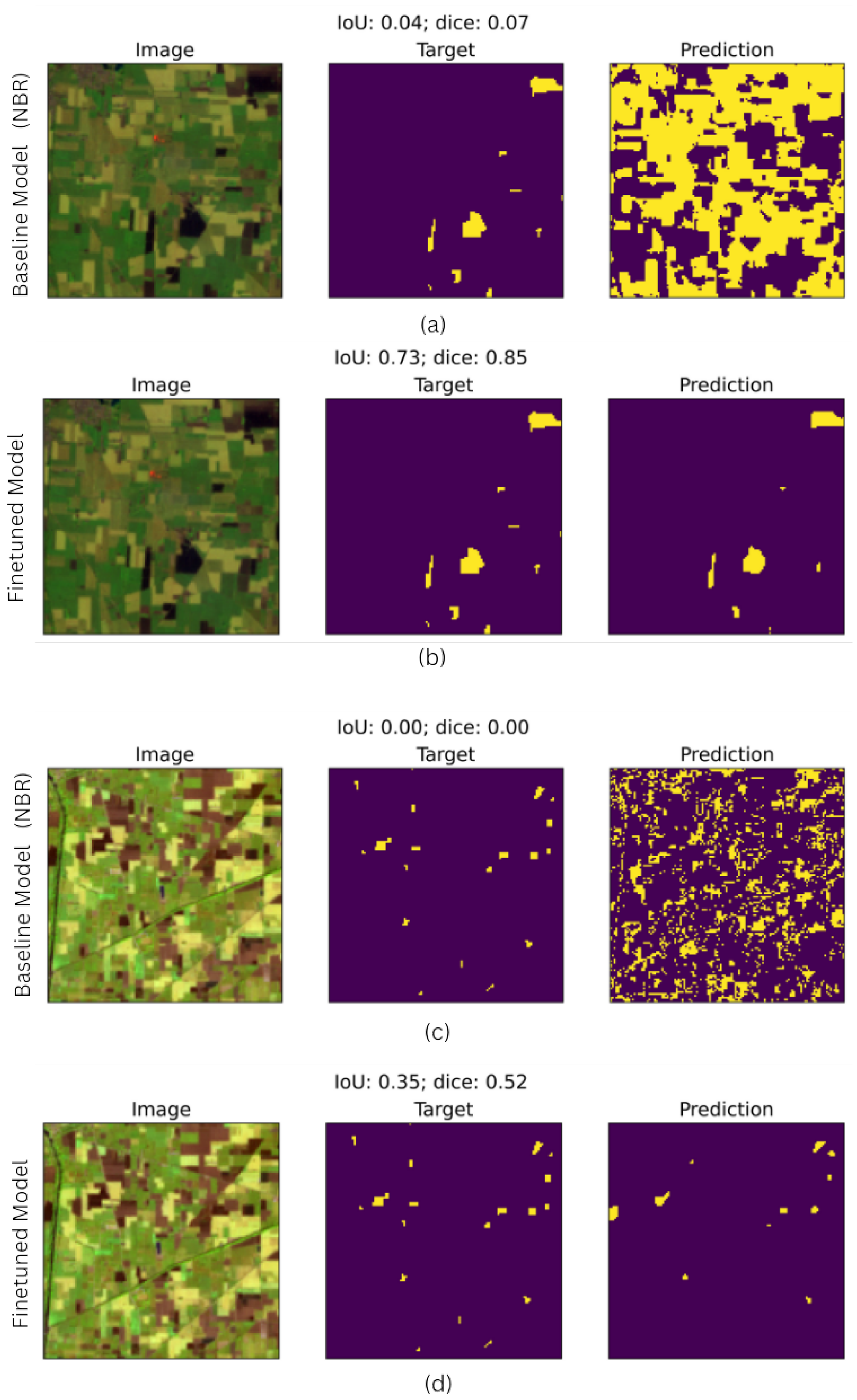
5.2. DL Model Prediction vs. Baseline Model (Normalized Burn Ratio Index Method)
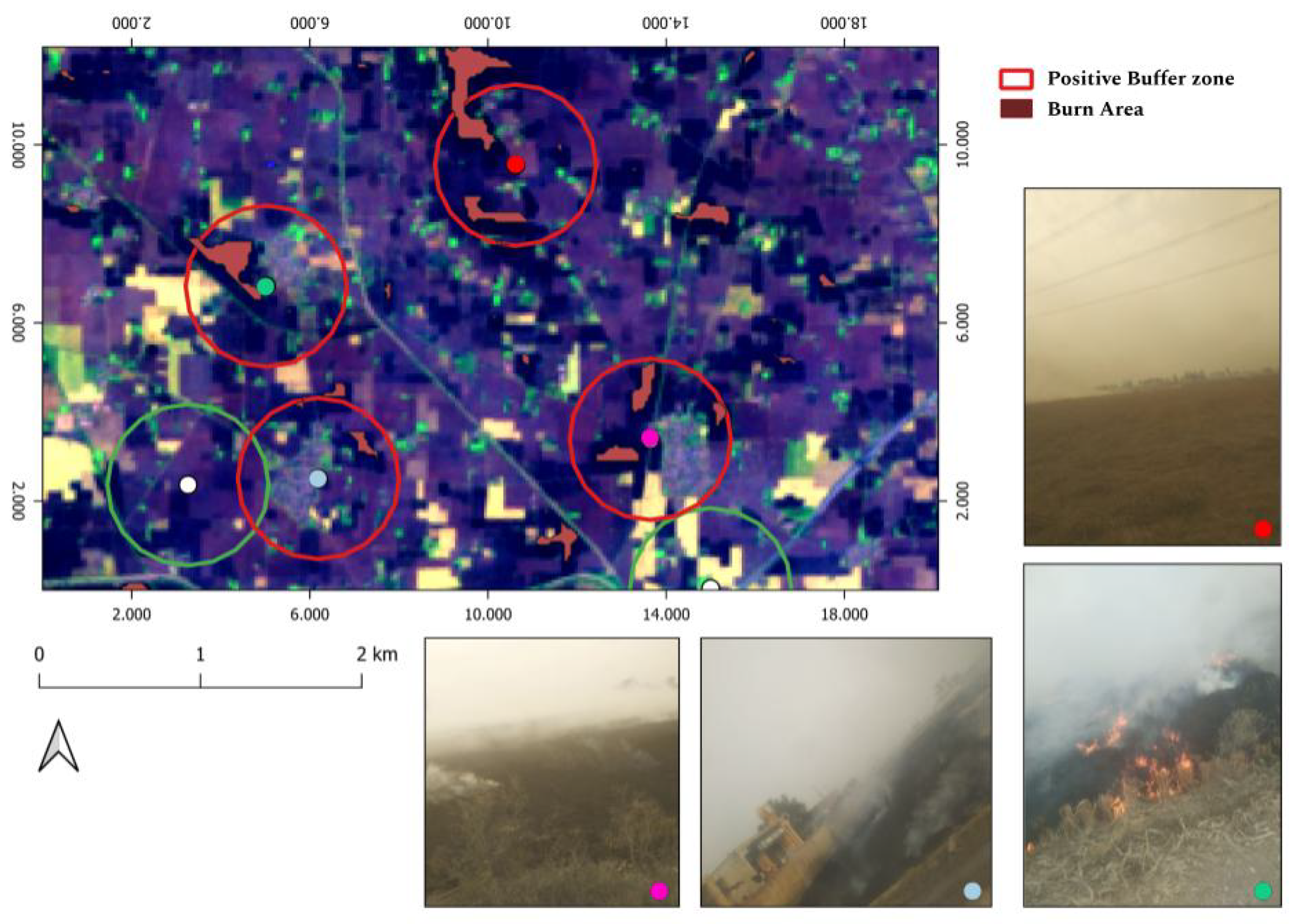
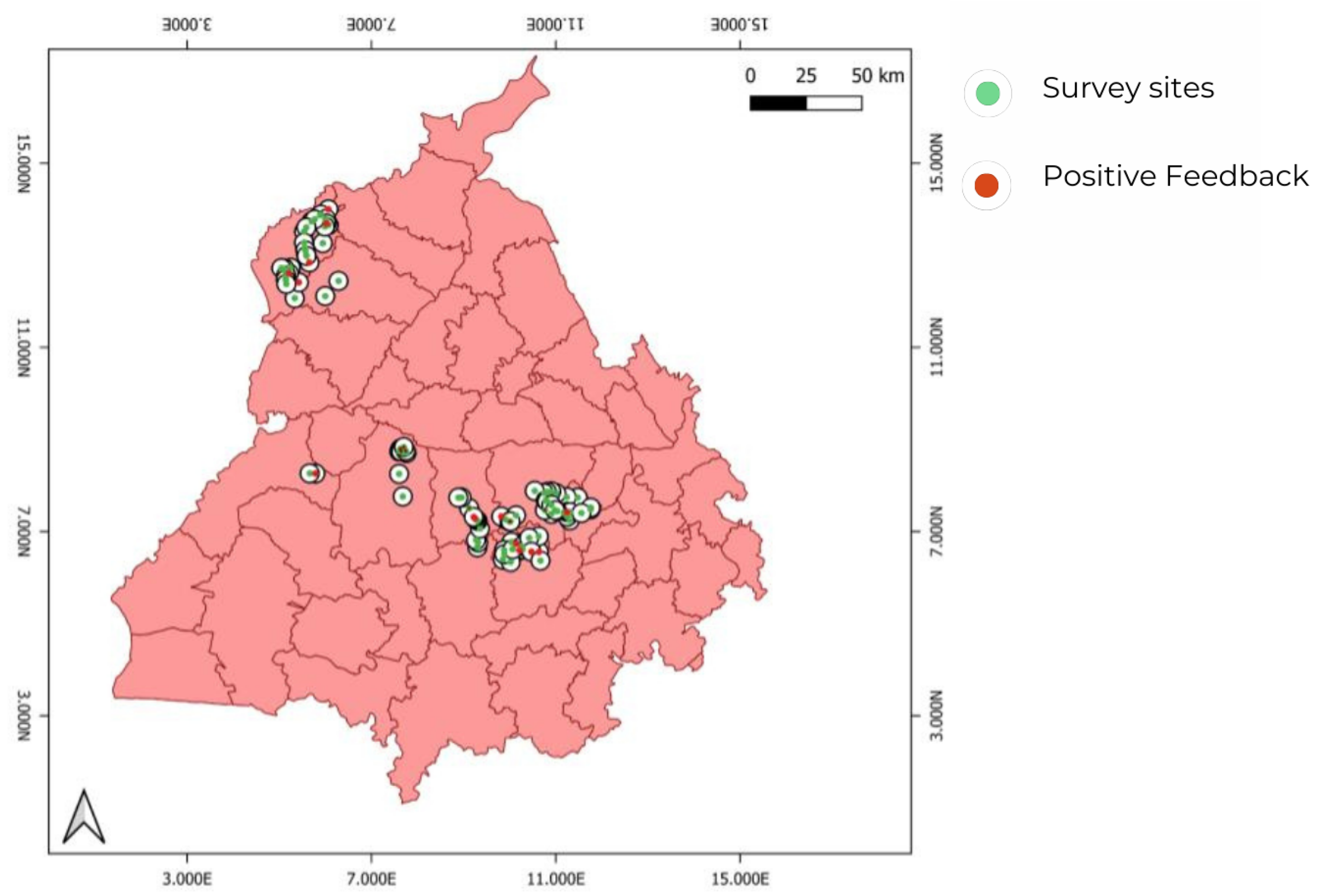
5.3. Site-Validation
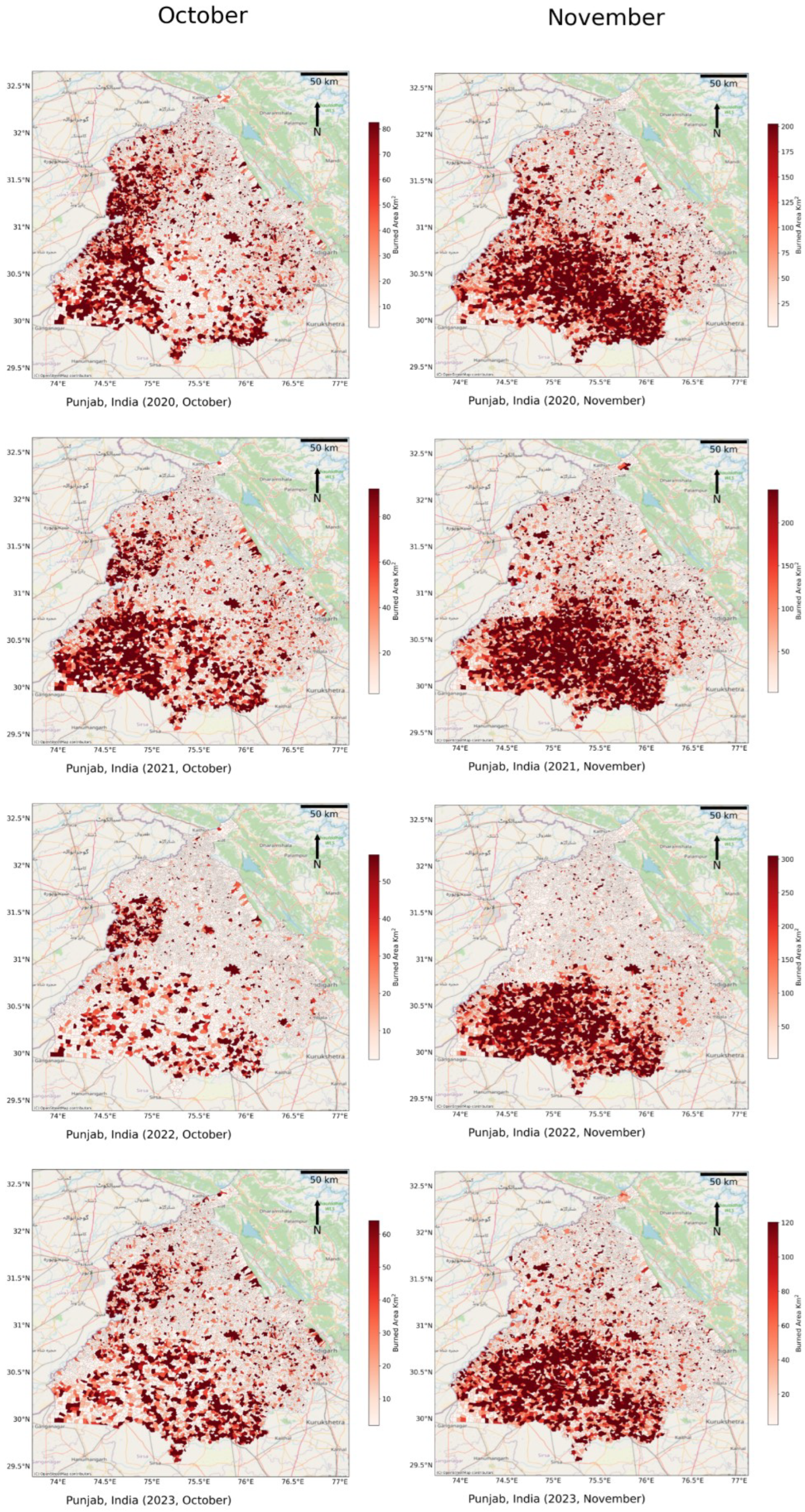
5.4. Spatiotemporal Distribution of Monthly Fire Activity for Post-Monsoon Burning Season (2020–2023))
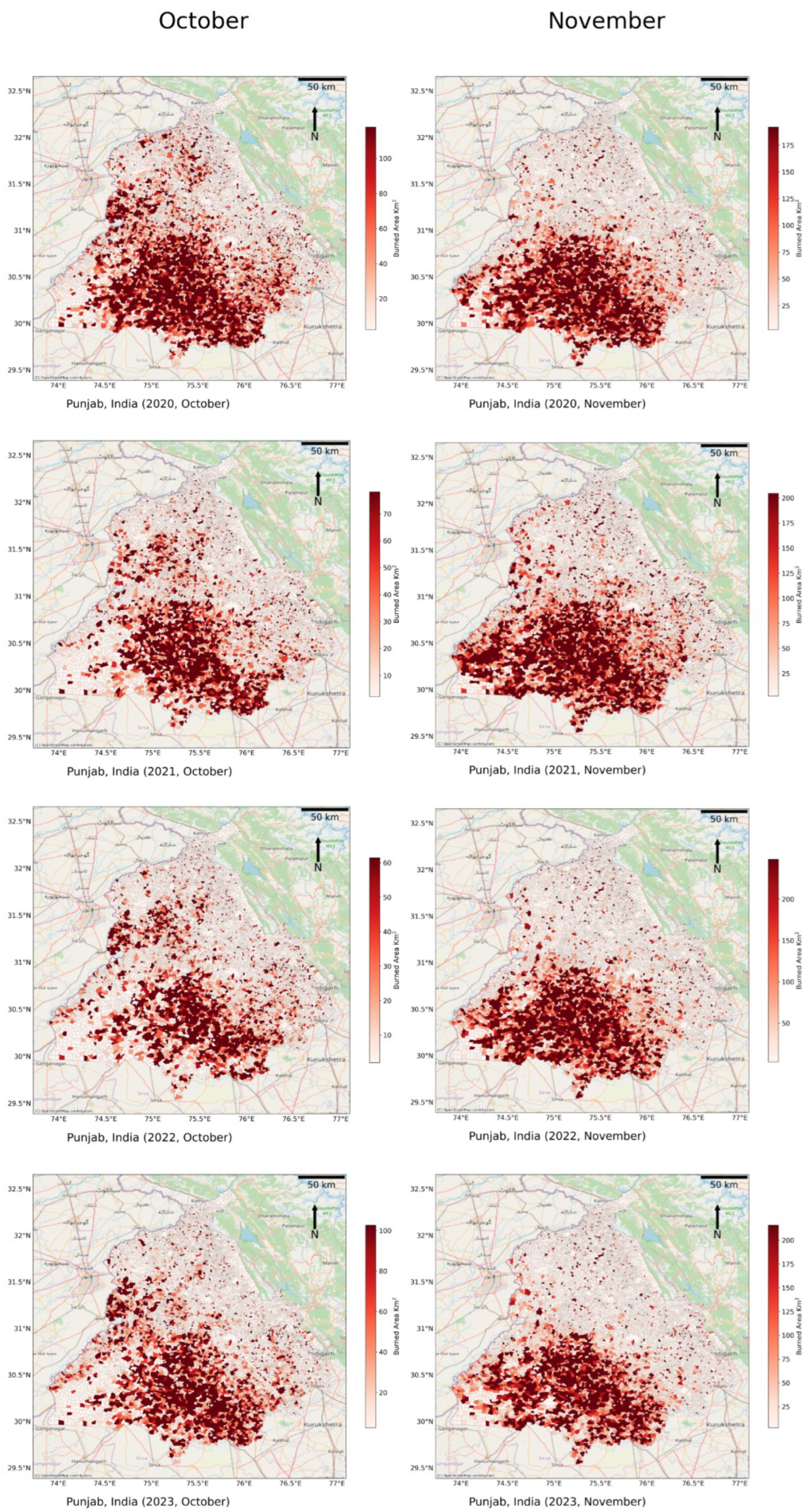
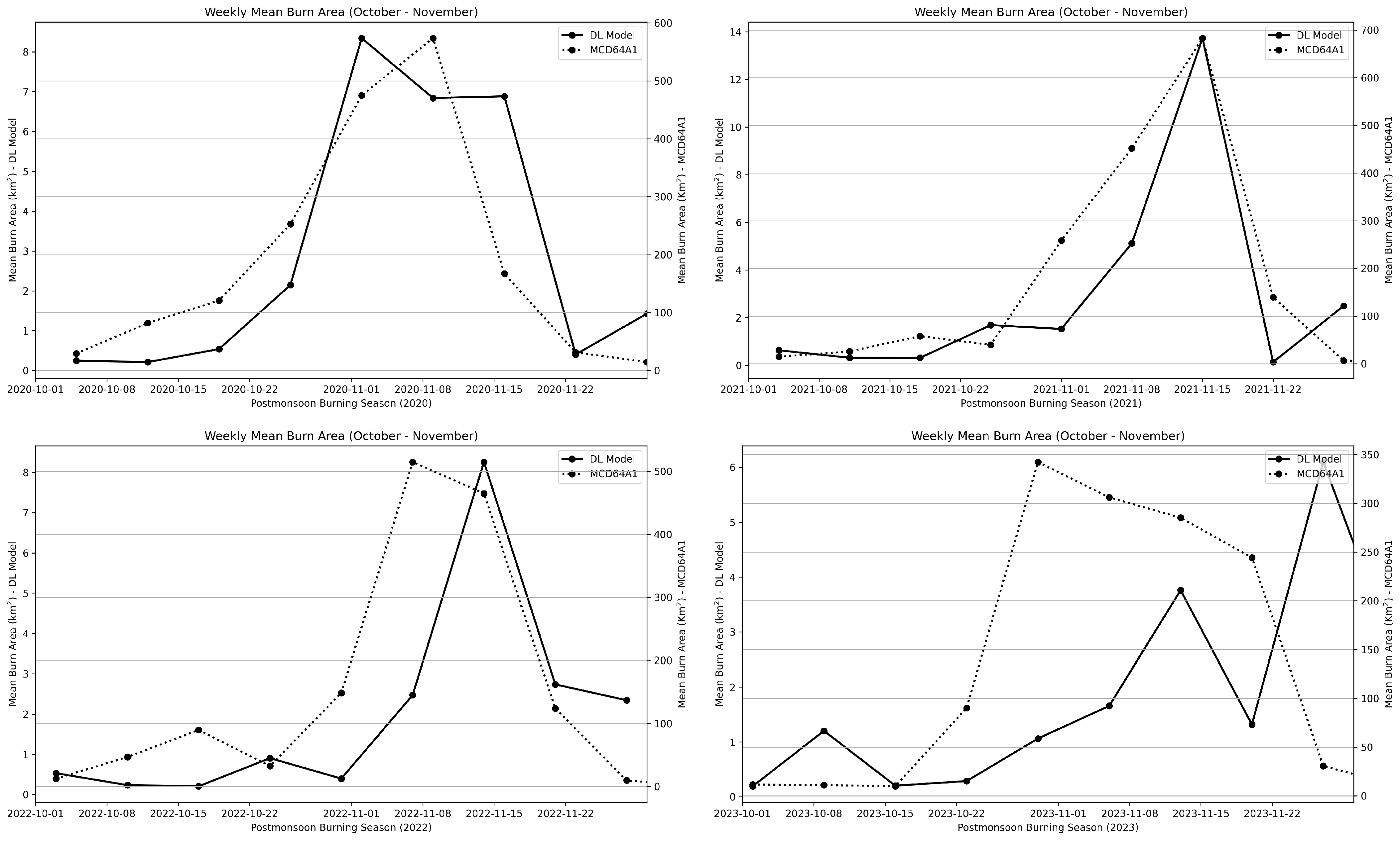
5.5. Comparison with MCD64A1 Burn Area Product
5.6. Limitations
6. Conclusions and Future Scope
Author Contributions
Funding
Data Availability Statement
Acknowledgments
Conflicts of Interest
Abbreviations
| DL | Deep Learning |
| CNN | Convolutional Neural Networks |
| NBR | Normalized Burn Ratio |
| MODIS | Moderate Resolution Imaging Spectroradiometer |
| VIIRS | Visible Infrared Imaging Radiometer Suite |
| NIR | Near Infrared |
| SWIR | Shortwave Infrared |
| ICNF | Institute for Nature Conservation and Forests |
| MSI | Multispectral Instrument |
| TOA | Top of Atmosphere |
| IoU | Intersection over Union |
| Annot-1 | Annotation 1 |
| Annot-2 | Annotation 2 |
| FDC | Fire Detection Counts |
Appendix A


Appendix B. Experimental Details

| Expt. | Descr. | Domain | GT-Data | lr | Batch Size | w | Encoder Layers | Epochs |
|---|---|---|---|---|---|---|---|---|
| A | raw model | Portugal (2016) | ICNF | 0.0003 | 32 | 0.0001 | unfrozen | 50 |
| B | Pretrained | Portugal (2017) | ICNF | 0.0003 | 32 | 0.0001 | unfrozen | 50 |
| C | Pretrained | Punjab (2020) | ICNF | 0.0003 | 32 | 0.0001 | unfrozen | 60 |
| D | TL-Pretrained | Punjab (2020) | Annot-1 | 3 | 32 | 0.0001 | unfrozen | 60 |
| E | TL-Pretrained | Punjab (2020) | Annot-1 | 0.0003 | 16 | 0.0001 | unfrozen | 50 |
| F | TL-Pretrained | Punjab (2020) | Annot-1 | 0.0003 | 8 | 0.0001 | unfrozen | 50 |
| G | TL-Pretrained | Punjab (2020) | Annot-2 | 0.0003 | 16 | 0.0001 | unfrozen | 45 |
| H | TL-Pretrained | Punjab (2020) | Annot-1 + Annot-2 | 0.0003 | 16 | 0.0001 | unfrozen | 60 |
| I | TL-Pretrained | Punjab (2020) | Annot-1 | 0.0003 | 16 | 0.001 | frozen | 25 + 5 * |
| J | TL-Pretrained | Punjab (2020) | Annot-1 | 0.0003 | 16 | 0.001 | frozen | 30 |
| K | TL-Pretrained | Punjab (2020) | Annot-2 | 0.0003 | 16 | 0.001 | frozen | 30 |
| L | TL-Pretrained | Punjab (2020) | Annot-1 | 0.0003 | 16 | 0.001 | frozen | 15 + 30 * |
| M | TL-Pretrained | Punjab (2020) | Annot-2 | 0.0003 | 16 | 0.001 | frozen | 15 + 25 * |
| Experiment | Domain | Type | Metric | Burned (%) | Non-Burned (%) |
|---|---|---|---|---|---|
| A | Portugal | Class | Precision | 81.6 | 96.7 |
| Recall | 80.9 | 96.9 | |||
| F1 | 81.2 | 96.8 | |||
| Overall | Accuracy (%) | 94.5 | |||
| Macro-F1 (%) | 89 | ||||
| IoU | 0.52 | ||||
| Dice | 0.60 | ||||
| B | Punjab | Class | Precision | 90.5 | 97.9 |
| Recall | 87.8 | 98.5 | |||
| F1 | 89.1 | 98.2 | |||
| Overall | Accuracy (%) | 96.9 | |||
| Macro-F1 (%) | 93.7 | ||||
| IoU | 0.54 | ||||
| Dice | 0.64 | ||||
| C | Punjab | Class | Precision | 95.1 | 99 |
| Recall | 94.9 | 99.1 | |||
| F1 | 94.8 | 99.0 | |||
| Overall | Accuracy (%) | 98.4 | |||
| Macro-F1 (%) | 95.0 | ||||
| IoU | 0.10 | ||||
| Dice | 0.13 | ||||
| D | Punjab | Class | Precision | 95 | 99 |
| Recall | 94 | 99 | |||
| F1 | 94 | 99 | |||
| Overall | Accuracy (%) | 98.3 | |||
| Macro-F1 (%) | 97 | ||||
| IoU | 0.44 | ||||
| Dice | 0.60 | ||||
| E | Punjab | Class | Precision | 95.1 | 99 |
| Recall | 94.5 | 99.1 | |||
| F1 | 94 | 99 | |||
| Overall | Accuracy (%) | 98.1 | |||
| Macro-F1 (%) | 97 | ||||
| IoU | 0.45 | ||||
| Dice | 0.60 | ||||
| F | Punjab | Class | Precision | 95 | 99 |
| Recall | 94 | 99 | |||
| F1 | 94 | 99 | |||
| Overall | Accuracy (%) | 99 | |||
| Macro-F1 (%) | 97.1 | ||||
| IoU | 0.46 | ||||
| Dice | 0.61 | ||||
| G | Punjab | Class | Precision | 95.4 | 99.1 |
| Recall | 95.3 | 99.1 | |||
| F1 | 95.3 | 99.08 | |||
| Overall | Accuracy (%) | 98.4 | |||
| Macro-F1 (%) | 97.2 | ||||
| IoU | 0.52 | ||||
| Dice | 0.64 | ||||
| H | Punjab | Class | Precision | 95.1 | 98.9 |
| Recall | 94.4 | 99 | |||
| F1 | 94.7 | 98.6 | |||
| Overall | Accuracy (%) | 98.7 | |||
| Macro-F1 (%) | 96.8 | ||||
| IoU | 0.42 | ||||
| Dice | 0.54 | ||||
| I | Punjab | Class | Precision | 95 | 99.1 |
| Recall | 95.2 | 99 | |||
| F1 | 95.1 | 99.1 | |||
| Overall | Accuracy (%) | 98.4 | |||
| Macro-F1 (%) | 97 | ||||
| IoU | 0.39 | ||||
| Dice | 0.54 | ||||
| J | Punjab | Class | Precision | 95.1 | 99 |
| Recall | 94.7 | 99.1 | |||
| F1 | 94.9 | 99 | |||
| Overall | Accuracy (%) | 98.3 | |||
| Macro-F1 (%) | 96.9 | ||||
| IoU | 0.43 | ||||
| Dice | 0.59 | ||||
| K | Punjab | Class | Precision | 96 | 99.2 |
| Recall | 95.7 | 99.2 | |||
| F1 | 95.9 | 99.2 | |||
| Overall | Accuracy (%) | 98.6 | |||
| Macro-F1 (%) | 97.5 | ||||
| IoU | 0.48 | ||||
| Dice | 0.58 | ||||
| L | Punjab | Class | Precision | 95.1 | 99 |
| Recall | 95 | 99.1 | |||
| F1 | 95 | 99 | |||
| Overall | Accuracy (%) | 98.4 | |||
| Macro-F1 (%) | 97 | ||||
| IoU | 0.43 | ||||
| Dice | 0.58 | ||||
| M | Punjab | Class | Precision | 96 | 98.2 |
| Recall | 95.8 | 99.2 | |||
| F1 | 95.9 | 99.2 | |||
| Overall | Accuracy (%) | 98.7 | |||
| Macro-F1 (%) | 97.6 | ||||
| IoU | 0.54 | ||||
| Dice | 0.64 | ||||
| Phase | Expt. | Domain | IoU (Val) | Dice (Val) | Model Accuracy IoU (Test) | Dice (Test) | Val_loss | Train_loss |
|---|---|---|---|---|---|---|---|---|
| I | A | Portugal | 0.62 | 0.72 | 0.50 | 0.59 | 0.34 | 0.33 |
| B | Portugal | 0.66 | 0.75 | 0.52 | 0.60 | 0.33 | 0.32 | |
| II | C | Punjab | 0.10 | 0.13 | ||||
| D | Punjab | 0.44 | 0.60 | 0.45 | 0.60 | 0.42 | 0.42 | |
| E | Punjab | 0.48 | 0.64 | 0.45 | 0.60 | 0.38 | 0.38 | |
| F | Punjab | 0.49 | 0.64 | 0.46 | 0.61 | 0.38 | 0.37 | |
| G | Punjab | 0.49 | 0.60 | 0.52 | 0.64 | 0.51 | 0.43 | |
| H | Punjab | 0.40 | 0.53 | 0.42 | 0.54 | 0.45 | 0.40 | |
| I | Punjab | 0.40 | 0.55 | 0.39 | 0.54 | 0.44 | 0.51 | |
| J | Punjab | 0.44 | 0.59 | 0.43 | 0.59 | 0.48 | 0.49 | |
| K | Punjab | 0.47 | 0.57 | 0.48 | 0.58 | 0.58 | 0.56 | |
| L | Punjab | 0.43 | 0.59 | 0.43 | 0.58 | 0.44 | 0.45 | |
| M | Punjab | 0.49 | 0.60 | 0.54 | 0.64 | 0.56 | 0.51 |
References
- Korontzi, S.; McCarty, J.; Loboda, T.; Kumar, S.; Justice, C. Global distribution of agricultural fires in croplands from 3 years of Moderate Resolution Imaging Spectroradiometer (MODIS) data. Glob. Biogeochem. Cycles 2006, 20, GB2021. [Google Scholar] [CrossRef]
- Cassou, E. Field Burning; Technical Report; World Bank: Washington, DC, USA, 2018. [Google Scholar] [CrossRef]
- Kumar, P.; Kumar, S.; Joshi, L. The Extent and Management of Crop Stubble. In Socioeconomic and Environmental Implications of Agricultural Residue Burning: A Case Study of Punjab, India; Springer: New Delhi, India, 2015; pp. 13–34. [Google Scholar] [CrossRef]
- Jethva, H.; Torres, O.; Field, R.D.; Lyapustin, A.; Gautam, R.; Kayetha, V. Connecting Crop Productivity, Residue Fires, and Air Quality over Northern India. Sci. Rep. 2019, 9, 16594. [Google Scholar] [CrossRef]
- Deshpande, M.V.; Kumar, N.; Pillai, D.; Krishna, V.V.; Jain, M. Greenhouse gas emissions from agricultural residue burning have increased by 75% since 2011 across India. Sci. Total. Environ. 2023, 904, 166944. [Google Scholar] [CrossRef]
- van der Werf, G.R.; Randerson, J.T.; Giglio, L.; Collatz, G.J.; Mu, M.; Kasibhatla, P.S.; Morton, D.C.; DeFries, R.S.; Jin, Y.; van Leeuwen, T.T. Global fire emissions and the contribution of deforestation, savanna, forest, agricultural, and peat fires (1997–2009). Atmos. Chem. Phys. 2010, 10, 11707–11735. [Google Scholar] [CrossRef]
- Singh, R.; Sinha, B.; Hakkim, H.; Sinha, V. Source apportionment of volatile organic compounds during paddy-residue burning season in north-west India reveals large pool of photochemically formed air toxics. Environ. Pollut. 2023, 338, 122656. [Google Scholar] [CrossRef] [PubMed]
- Dhaka, S.K.; Chetna; Kumar, V.; Panwar, V.; Dimri, A.; Singh, N.; Patra, P.K.; Matsumi, Y.; Takigawa, M.; Nakayama, T.; et al. PM2. 5 diminution and haze events over Delhi during the COVID-19 lockdown period: An interplay between the baseline pollution and meteorology. Sci. Rep. 2020, 10, 13442. [Google Scholar] [CrossRef] [PubMed]
- Hall, J.V.; Loboda, T.V. Quantifying the Potential for Low-Level Transport of Black Carbon Emissions from Cropland Burning in Russia to the Snow-Covered Arctic. Front. Earth Sci. 2017, 5, 109. [Google Scholar] [CrossRef]
- Andreae, M.O. Biomass Burning: Its History, Use, and Distribution and Its Impact on Environmental Quality and Global Climate. In Global Biomass Burning; The MIT Press: Cambridge, MA, USA, 1991; pp. 3–21. [Google Scholar] [CrossRef]
- Hall, J.V.; Loboda, T.V.; Giglio, L.; McCarty, G.W. A MODIS-based burned area assessment for Russian croplands: Mapping requirements and challenges. Remote Sens. Environ. 2016, 184, 506–521. [Google Scholar] [CrossRef]
- Seiler, W.; Crutzen, P.J. Estimates of gross and net fluxes of carbon between the biosphere and the atmosphere from biomass burning. Clim. Chang. 1980, 2, 207–247. [Google Scholar] [CrossRef]
- Van Der Werf, G.R.; Randerson, J.T.; Giglio, L.; Gobron, N.; Dolman, A. Climate controls on the variability of fires in the tropics and subtropics. Glob. Biogeochem. Cycles 2008, 22. [Google Scholar] [CrossRef]
- Ramo, R.; Roteta, E.; Bistinas, I.; Van Wees, D.; Bastarrika, A.; Chuvieco, E.; Van der Werf, G.R. African burned area and fire carbon emissions are strongly impacted by small fires undetected by coarse resolution satellite data. Proc. Natl. Acad. Sci. USA 2021, 118, e2011160118. [Google Scholar] [CrossRef] [PubMed]
- Andela, N.; Morton, D.C.; Giglio, L.; Paugam, R.; Chen, Y.; Hantson, S.; Van Der Werf, G.R.; Randerson, J.T. The Global Fire Atlas of individual fire size, duration, speed and direction. Earth Syst. Sci. Data 2019, 11, 529–552. [Google Scholar] [CrossRef]
- Konovalov, I.; Beekmann, M.; Kuznetsova, I.N.; Yurova, A.; Zvyagintsev, A. Atmospheric impacts of the 2010 Russian wildfires: Integrating modelling and measurements of an extreme air pollution episode in the Moscow region. Atmos. Chem. Phys. 2011, 11, 10031–10056. [Google Scholar] [CrossRef]
- Archibald, S.; Lehmann, C.E.; Gómez-Dans, J.L.; Bradstock, R.A. Defining pyromes and global syndromes of fire regimes. Proc. Natl. Acad. Sci. USA 2013, 110, 6442–6447. [Google Scholar] [CrossRef] [PubMed]
- Chuvieco, E.; Mouillot, F.; van der Werf, G.R.; San Miguel, J.; Tanase, M.; Koutsias, N.; García, M.; Yebra, M.; Padilla, M.; Gitas, I.; et al. Historical background and current developments for mapping burned area from satellite Earth observation. Remote Sens. Environ. 2019, 225, 45–64. [Google Scholar] [CrossRef]
- GCOS. The global observing system for climate: Implementation needs. World Meteorol. Organ. 2016, 200, 316. [Google Scholar]
- Giglio, L.; Boschetti, L.; Roy, D.P.; Humber, M.L.; Justice, C.O. The Collection 6 MODIS burned area mapping algorithm and product. Remote Sens. Environ. 2018, 217, 72–85. [Google Scholar] [CrossRef]
- Roteta, E.; Bastarrika, A.; Padilla, M.; Storm, T.; Chuvieco, E. Development of a Sentinel-2 burned area algorithm: Generation of a small fire database for sub-Saharan Africa. Remote Sens. Environ. 2019, 222, 1–17. [Google Scholar] [CrossRef]
- Roy, D.P.; Boschetti, L. Southern Africa validation of the MODIS, L3JRC, and GlobCarbon burned-area products. IEEE Trans. Geosci. Remote Sens. 2009, 47, 1032–1044. [Google Scholar] [CrossRef]
- Roy, D.; Boschetti, L.; Justice, C.; Ju, J. The collection 5 MODIS burned area product—Global evaluation by comparison with the MODIS active fire product. Remote Sens. Environ. 2008, 112, 3690–3707. [Google Scholar] [CrossRef]
- Giglio, L.; Loboda, T.; Roy, D.P.; Quayle, B.; Justice, C.O. An active-fire based burned area mapping algorithm for the MODIS sensor. Remote Sens. Environ. 2009, 113, 408–420. [Google Scholar] [CrossRef]
- Giglio, L.; Kendall, J.D.; Mack, R. A multi-year active fire dataset for the tropics derived from the TRMM VIRS. Int. J. Remote Sens. 2003, 24, 4505–4525. [Google Scholar] [CrossRef]
- McCarty, J.L.; Korontzi, S.; Justice, C.O.; Loboda, T. The spatial and temporal distribution of crop residue burning in the contiguous United States. Sci. Total. Environ. 2009, 407, 5701–5712. [Google Scholar] [CrossRef]
- Ouattara, B.; Thiel, M.; Sponholz, B.; Paeth, H.; Yebra, M.; Mouillot, F.; Kacic, P.; Hackman, K. Enhancing burned area monitoring with VIIRS dataset: A case study in Sub-Saharan Africa. Sci. Remote Sens. 2024, 10, 100165. [Google Scholar] [CrossRef]
- Giglio, L.; Boschetti, L.; Roy, D.; Hoffmann, A.A.; Humber, M.; Hall, J.V. Collection 6 Modis Burned Area Product User’s Guide Version 1.0; NASA EOSDIS Land Processes DAAC: Sioux Falls, SD, USA, 2016; pp. 11–27. [Google Scholar]
- Wieland, M.; Li, Y.; Martinis, S. Multi-sensor cloud and cloud shadow segmentation with a convolutional neural network. Remote Sens. Environ. 2019, 230, 111203. [Google Scholar] [CrossRef]
- Xie, Y.; Liu, S.; Chen, H.; Cao, S.; Zhang, H.; Feng, D.; Wan, Q.; Zhu, J.; Zhu, Q. Localization, balance and affinity: A stronger multifaceted collaborative salient object detector in remote sensing images. IEEE Trans. Geosci. Remote Sens. 2024, 63, 4700117. [Google Scholar] [CrossRef]
- Minaee, S.; Boykov, Y.; Porikli, F.; Plaza, A.; Kehtarnavaz, N.; Terzopoulos, D. Image segmentation using deep learning: A survey. IEEE Trans. Pattern Anal. Mach. Intell. 2021, 44, 3523–3542. [Google Scholar] [CrossRef] [PubMed]
- Al-Rawi, K.R.; Casanova, J.L.; Calle, A. Burned area mapping system and fire detection system, based on neural networks and NOAA-AVHRR imagery. Int. J. Remote Sens. 2001, 22, 2015–2032. [Google Scholar] [CrossRef]
- Brivio, P.A.; Maggi, M.; Binaghi, E.; Gallo, I. Mapping burned surfaces in Sub-Saharan Africa based on multi-temporal neural classification. Int. J. Remote Sens. 2003, 24, 4003–4016. [Google Scholar] [CrossRef]
- Huppertz, R.; Nakalembe, C.; Kerner, H.; Lachyan, R.; Rischard, M. Using transfer learning to study burned area dynamics: A case study of refugee settlements in West Nile, Northern Uganda, 2021. arXiv 2021, arXiv:2107.14372. [Google Scholar]
- Wieland, M.; Martinis, S.; Kiefl, R.; Gstaiger, V. Semantic segmentation of water bodies in very high-resolution satellite and aerial images. Remote Sens. Environ. 2023, 287, 113452. [Google Scholar] [CrossRef]
- Maggiori, E.; Tarabalka, Y.; Charpiat, G.; Alliez, P. Convolutional Neural Networks for Large-Scale Remote-Sensing Image Classification. IEEE Trans. Geosci. Remote Sens. 2017, 55, 645–657. [Google Scholar] [CrossRef]
- Rustowicz, R.; Cheong, R.; Wang, L.; Ermon, S.; Burke, M.; Lobell, D. Semantic Segmentation of Crop Type in Africa: A Novel Dataset and Analysis of Deep Learning Methods. In Proceedings of the CVPR Workshops, Long Beach, CA, USA, 16–20 June 2019. [Google Scholar]
- Chetna, N.; Devi, M. Forecasting of Pre-harvest Wheat Yield using Discriminant Function Analysis of Meteorological Parameters of Kurukshetra District of Haryana. J. Agric. Res. Technol. 2022, 47, 67–72. [Google Scholar] [CrossRef]
- Pinto, M.M.; Trigo, R.M.; Trigo, I.F.; DaCamara, C.C. A Practical Method for High-Resolution Burned Area Monitoring Using Sentinel-2 and VIIRS. Remote Sens. 2021, 13, 1608. [Google Scholar] [CrossRef]
- Knopp, L.; Wieland, M.; Rättich, M.; Martinis, S. A Deep Learning Approach for Burned Area Segmentation with Sentinel-2 Data. Remote Sens. 2020, 12, 2422. [Google Scholar] [CrossRef]
- Kumar, R.; Barth, M.; Pfister, G.; Nair, V.; Ghude, S.D.; Ojha, N. What controls the seasonal cycle of black carbon aerosols in India? J. Geophys. Res. Atmos. 2015, 120, 7788–7812. [Google Scholar] [CrossRef]
- National Remote Sensing Centre (NRSC), ISRO. Land Use Land Cover Digital Database. Natural Resources Census Project, 2024. Available online: https://bhuvan-app1.nrsc.gov.in/2dresources/thematic/LULC503/MAP/PB.jpg (accessed on 25 February 2025).
- Kaskaoutis, D.; Kumar, S.; Sharma, D.; Singh, R.P.; Kharol, S.; Sharma, M.; Singh, A.; Singh, S.; Singh, A.; Singh, D. Effects of crop residue burning on aerosol properties, plume characteristics, and long-range transport over northern India. J. Geophys. Res. Atmos. 2014, 119, 5424–5444. [Google Scholar] [CrossRef]
- Ravindra, K.; Singh, T.; Mor, S. Emissions of air pollutants from primary crop residue burning in India and their mitigation strategies for cleaner emissions. J. Clean. Prod. 2019, 208, 261–273. [Google Scholar] [CrossRef]
- Wang, J.; Christopher, S.A.; Nair, U.S.; Reid, J.S.; Prins, E.M.; Szykman, J.; Hand, J.L. Mesoscale modeling of Central American smoke transport to the United States: 1. “Top-down” assessment of emission strength and diurnal variation impacts. J. Geophys. Res. Atmos. 2006, 111. [Google Scholar] [CrossRef]
- Sharma, A.R.; Kharol, S.K.; Badarinath, K.V.S.; Singh, D. Impact of agriculture crop residue burning on atmospheric aerosol loading – a study over Punjab State, India. Ann. Geophys. 2010, 28, 367–379. [Google Scholar] [CrossRef]
- Ronneberger, O.; Fischer, P.; Brox, T. U-Net: Convolutional Networks for Biomedical Image Segmentation. In Proceedings of the Medical Image Computing and Computer-Assisted Intervention—MICCAI 2015; Navab, N., Hornegger, J., Wells, W.M., Frangi, A.F., Eds.; Springer International Publishing: Cham, Switzerland, 2015; pp. 234–241. [Google Scholar] [CrossRef]
- Main-Knorn, M.; Pflug, B.; Louis, J.; Debaecker, V.; Müller-Wilm, U.; Gascon, F. Sen2Cor for Sentinel-2. In Proceedings of the Image and Signal Processing for Remote Sensing XXIII; Bruzzone, L., Ed.; International Society for Optics and Photonics, SPIE: Bellingham, WA, USA, 2017; Volume 10427, p. 1042704. [Google Scholar] [CrossRef]
- Sentinel-2 ESA’s Optical High-Resolution Mission for GMES Operational Services (ESA SP-1322/2 March 2012). Available online: https://sentinel.esa.int/documents/247904/349490/S2_SP-1322_2.pdf (accessed on 4 August 2024).
- Turco, M.; Jerez, S.; Augusto, S.; Tarín-Carrasco, P.; Ratola, N.; Jiménez-Guerrero, P.; Trigo, R.M. Climate drivers of the 2017 devastating fires in Portugal. Sci. Rep. 2019, 9, 13886. [Google Scholar] [CrossRef] [PubMed]
- Menezes, L.S.; Russo, A.; Libonati, R.; Trigo, R.M.; Pereira, J.M.; Benali, A.; Ramos, A.M.; Gouveia, C.M.; Morales Rodriguez, C.A.; Deus, R. Lightning-induced fire regime in Portugal based on satellite-derived and in situ data. Agric. For. Meteorol. 2024, 355, 110108. [Google Scholar] [CrossRef]
- Copernicus Data Space Ecosystem-API-OData. Available online: https://documentation.dataspace.copernicus.eu/APIs/OData.html (accessed on 2 August 2024).
- Institute of Conservation of Nature and Forest. Available online: https://sig.icnf.pt/portal/home/item.html?id=983c4e6c4d5b4666b258a3ad5f3ea5af#overview (accessed on 2 August 2024).
- Vadrevu, K.; Lasko, K. Intercomparison of MODIS AQUA and VIIRS I-Band Fires and Emissions in an Agricultural Landscape—Implications for Air Pollution Research. Remote Sens. 2018, 10, 978. [Google Scholar] [CrossRef] [PubMed]
- Liu, T.; Marlier, M.E.; Karambelas, A.; Jain, M.; Singh, S.; Singh, M.K.; Gautam, R.; DeFries, R.S. Missing emissions from post-monsoon agricultural fires in northwestern India: Regional limitations of MODIS burned area and active fire products. Environ. Res. Commun. 2019, 1, 011007. [Google Scholar] [CrossRef]
- Key, C.; Benson, N. Measuring and remote sensing of burn severity. In Proceedings of the Joint Fire Science Conference and Workshop; Proceedings: ‘Crossing the Millennium: Integrating Spatial Technologies and Ecological Principles for a New Age in Fire Management’, Boise, ID, USA, 15–17 June 1999. [Google Scholar]
- Keeley, J. Fire intensity, fire severity and burn severity: A brief review and suggested usage. Int. J. Wildland Fire 2009, 18, 116–126. [Google Scholar] [CrossRef]
- He, K.; Zhang, X.; Ren, S.; Sun, J. Deep Residual Learning for Image Recognition. In Proceedings of the 2016 IEEE Conference on Computer Vision and Pattern Recognition (CVPR), Las Vegas, NV, USA, 27–30 June 2016; pp. 770–778. [Google Scholar] [CrossRef]
- Kugelman, J.; Allman, J.; Read, S.A.; Vincent, S.J.; Tong, J.; Kalloniatis, M.; Chen, F.K.; Collins, M.J.; Alonso-Caneiro, D. A comparison of deep learning U-Net architectures for posterior segment OCT retinal layer segmentation. Sci. Rep. 2022, 12, 14888. [Google Scholar] [CrossRef]
- viso.ai. U-Net: A Comprehensive Guide to Its Architecture and Applications. 2024. Available online: https://viso.ai/deep-learning/u-net-a-comprehensive-guide-to-its-architecture-and-applications/ (accessed on 19 February 2025).
- Zhao, H.; Shi, J.; Qi, X.; Wang, X.; Jia, J. Pyramid Scene Parsing Network. In Proceedings of the 2017 IEEE Conference on Computer Vision and Pattern Recognition (CVPR), Honolulu, HI, USA, 21–26 July 2017; pp. 6230–6239. [Google Scholar] [CrossRef]
- He, F.; Liu, T.; Tao, D. Control Batch Size and Learning Rate to Generalize Well: Theoretical and Empirical Evidence. Adv. Neural Inf. Process. Syst. 2019, 32. Available online: https://proceedings.neurips.cc/paper_files/paper/2019/file/dc6a70712a252123c40d2adba6a11d84-Paper.pdf (accessed on 25 February 2025).
- Li, H.; Parikh, N.A.; He, L. A novel transfer learning approach to enhance deep neural network classification of brain functional connectomes. Front. Neurosci. 2018, 12, 491. [Google Scholar] [CrossRef]
- Kingma, D.P.; Ba, J. Adam: A Method for Stochastic Optimization. In Proceedings of the 3rd International Conference on Learning Representations, ICLR 2015, San Diego, CA, USA, 7–9 May 2015. [Google Scholar] [CrossRef]
- Ruby, U.; Yendapalli, V. Binary cross entropy with deep learning technique for image classification. Int. J. Adv. Trends Comput. Sci. Eng. 2020, 9, 5393. [Google Scholar] [CrossRef]
- Wisteria/BDEC-01 Supercomputer System. Available online: https://www.cc.u-tokyo.ac.jp/en/supercomputer/wisteria/service/ (accessed on 3 August 2024).
- Pereira, P.; Silveira, M. Cross-Modal Transfer Learning Methods for Alzheimer’s Disease Diagnosis. In Proceedings of the 2022 44th Annual International Conference of the IEEE Engineering in Medicine & Biology Society (EMBC), Glasgow, UK, 11–15 July 2022; IEEE: Piscataway, NJ, USA, 2022; pp. 3789–3792. [Google Scholar] [CrossRef]
- Garcia-Garcia, A.; Orts-Escolano, S.; Oprea, S.; Villena-Martinez, V.; Garcia-Rodriguez, J. A Review on Deep Learning Techniques Applied to Semantic Segmentation. arXiv 2017, arXiv:1704.06857. [Google Scholar]
- Zou, K.H.; Warfield, S.K.; Bharatha, A.; Tempany, C.M.; Kaus, M.R.; Haker, S.J.; Wells, W.M.; Jolesz, F.A.; Kikinis, R. Statistical validation of image segmentation quality based on a spatial overlap index1: Scientific reports. Acad. Radiol. 2004, 11, 178–189. [Google Scholar] [CrossRef] [PubMed]
- Szpakowski, D.M.; Jensen, J.L.R. A Review of the Applications of Remote Sensing in Fire Ecology. Remote Sens. 2019, 11, 2638. [Google Scholar] [CrossRef]
- Gamper, J.; Koohbanani, N.A.; Benes, K.; Graham, S.; Jahanifar, M.; Khurram, S.A.; Azam, A.; Hewitt, K.; Rajpoot, N. PanNuke Dataset Extension, Insights and Baselines. arXiv 2020, arXiv:2003.10778. [Google Scholar]
- Chicco, D.; Jurman, G. The advantages of the Matthews correlation coefficient (MCC) over F1 score and accuracy in binary classification evaluation. BMC Genom. 2020, 21, 1–13. [Google Scholar] [CrossRef]
- Yosinski, J.; Clune, J.; Bengio, Y.; Lipson, H. How transferable are features in deep neural networks? Adv. Neural Inf. Process. Syst. 2014, 27. [Google Scholar] [CrossRef]
- Howard, J.; Ruder, S. Universal language model fine-tuning for text classification. arXiv 2018, arXiv:1801.06146. [Google Scholar]
- Tajbakhsh, N.; Shin, J.Y.; Gurudu, S.R.; Hurst, R.T.; Kendall, C.B.; Gotway, M.B.; Liang, J. Convolutional neural networks for medical image analysis: Full training or fine tuning? IEEE Trans. Med. Imaging 2016, 35, 1299–1312. [Google Scholar] [CrossRef] [PubMed]
- Zhang, Z.; Wu, C.; Coleman, S.; Kerr, D. DENSE-INception U-net for medical image segmentation. Comput. Methods Programs Biomed. 2020, 192, 105395. [Google Scholar] [CrossRef]
- Farhadi, H.; Ebadi, H.; Kiani, A. Badi: A Novel Burned Area Detection Index for Sentinel-2 Imagery Using Google Earth Engine Platform. ISPRS Ann. Photogramm. Remote Sens. Spat. Inf. Sci. 2023, X-4/W1-2022, 179–186. [Google Scholar] [CrossRef]
- Singh, G.; Kant, Y.; Dadhwal, V. Remote sensing of crop residue burning in Punjab (India): A study on burned area estimation using multi-sensor approach. Geocarto Int. 2009, 24, 273–292. [Google Scholar] [CrossRef]
- Pinto, M.M.; Libonati, R.; Trigo, R.M.; Trigo, I.F.; DaCamara, C.C. A deep learning approach for mapping and dating burned areas using temporal sequences of satellite images. ISPRS J. Photogramm. Remote Sens. 2020, 160, 260–274. [Google Scholar] [CrossRef]
- Daily Updates from Intensive Observation Campaign 2023 Autumn. Available online: https://aakash-rihn.org/en/campaign2023/ (accessed on 4 August 2024).
- Mangaraj1, P.; Matsumi, Y.; Nakayama, T.; Biswal, A.; Yamaji, K.; Araki, H.; Yasutomi, N.; Takigawa, M.; Patra, P.K.; Hayashida, S.; et al. Weak coupling of observed surface PM2.5 in Delhi-NCR with rice crop residue burning in Punjab and Haryana. NPJ Clim. Atmos. Sci. 2025, 8, 18. [Google Scholar] [CrossRef]
- Ministry of Environment, Forest and Climate Change. Paddy Harvesting Season 2023 Comes to an End Witnessing Significant Decrease in Stubble Burning with Efforts Made Towards Management of Paddy Straw for the Current Season. 2023. Available online: https://pib.gov.in/PressReleaseIframePage.aspx?PRID=1981276 (accessed on 25 February 2025).
- Wiedinmyer, C.; Kimura, Y.; McDonald-Buller, E.C.; Emmons, L.K.; Buchholz, R.R.; Tang, W.; Seto, K.; Joseph, M.B.; Barsanti, K.C.; Carlton, A.G.; et al. The Fire Inventory from NCAR version 2.5: An updated global fire emissions model for climate and chemistry applications. Geosci. Model Dev. 2023, 16, 3873–3891. [Google Scholar] [CrossRef]
- Campagnolo, M.; Libonati, R.; Rodrigues, J.; Pereira, J. A comprehensive characterization of MODIS daily burned area mapping accuracy across fire sizes in tropical savannas. Remote Sens. Environ. 2021, 252, 112115. [Google Scholar] [CrossRef]
- Pan, S.J.; Yang, Q. A survey on transfer learning. IEEE Trans. Knowl. Data Eng. 2009, 22, 1345–1359. [Google Scholar] [CrossRef]
| Band | Description | Bandwidth (nm) | Central Wavelength (nm) | Spatial Resolution (m) |
|---|---|---|---|---|
| 1 | Aerosol | 20 | 443 | 60 |
| 2 | Blue | 65 | 490 | 10 |
| 3 | Green | 35 | 560 | 10 |
| 4 | Red | 30 | 665 | 10 |
| 5 | Vegetation edge | 15 | 705 | 20 |
| 6 | Vegetation edge | 15 | 740 | 20 |
| 7 | Vegetation edge | 20 | 783 | 20 |
| 8a | NIR | 115 | 842 | 10 |
| 8b | Narrow NIR | 20 | 865 | 20 |
| 9 | Water vapor | 20 | 945 | 60 |
| 10 | Circus | 30 | 1380 | 60 |
| 11 | SWIR1 | 90 | 1610 | 20 |
| 12 | SWIR2 | 180 | 2190 | 20 |
| Model | Domain | Type | Metric | Burned (%) | Non-Burned (%) |
|---|---|---|---|---|---|
| DL-Model | Portugal | class | Precision | 81.6 | 96.7 |
| Recall | 80.9 | 96.9 | |||
| F1 | 81.2 | 96.8 | |||
| overall | Accuracy (%) | 94.5 | |||
| Macro-F1 (%) | 89 | ||||
| IoU | 0.52 | ||||
| Dice | 0.60 | ||||
| DL-Model | Punjab | class | Precision | 96 | 98.2 |
| Recall | 95.8 | 99.2 | |||
| F1 | 95.9 | 99.2 | |||
| overall | Accuracy (%) | 98.7 | |||
| Macro-F1 (%) | 97.6 | ||||
| IoU | 0.54 | ||||
| Dice | 0.64 | ||||
| Baseline (NBR) | Punjab | class | Precision | 90.8 | 90.1 |
| Recall | 49.1 | 98.9 | |||
| F1 | 63.5 | 94.3 | |||
| overall | Accuracy (%) | 91 | |||
| Macro-F1 (%) | 78 | ||||
| IoU | 0.03 | ||||
| Dice | 0.05 | ||||
Disclaimer/Publisher’s Note: The statements, opinions and data contained in all publications are solely those of the individual author(s) and contributor(s) and not of MDPI and/or the editor(s). MDPI and/or the editor(s) disclaim responsibility for any injury to people or property resulting from any ideas, methods, instructions or products referred to in the content. |
© 2025 by the authors. Licensee MDPI, Basel, Switzerland. This article is an open access article distributed under the terms and conditions of the Creative Commons Attribution (CC BY) license (https://creativecommons.org/licenses/by/4.0/).
Share and Cite
Anand, A.; Imasu, R.; Dhaka, S.K.; Patra, P.K. Domain Adaptation and Fine-Tuning of a Deep Learning Segmentation Model of Small Agricultural Burn Area Detection Using High-Resolution Sentinel-2 Observations: A Case Study of Punjab, India. Remote Sens. 2025, 17, 974. https://doi.org/10.3390/rs17060974
Anand A, Imasu R, Dhaka SK, Patra PK. Domain Adaptation and Fine-Tuning of a Deep Learning Segmentation Model of Small Agricultural Burn Area Detection Using High-Resolution Sentinel-2 Observations: A Case Study of Punjab, India. Remote Sensing. 2025; 17(6):974. https://doi.org/10.3390/rs17060974
Chicago/Turabian StyleAnand, Anamika, Ryoichi Imasu, Surendra K. Dhaka, and Prabir K. Patra. 2025. "Domain Adaptation and Fine-Tuning of a Deep Learning Segmentation Model of Small Agricultural Burn Area Detection Using High-Resolution Sentinel-2 Observations: A Case Study of Punjab, India" Remote Sensing 17, no. 6: 974. https://doi.org/10.3390/rs17060974
APA StyleAnand, A., Imasu, R., Dhaka, S. K., & Patra, P. K. (2025). Domain Adaptation and Fine-Tuning of a Deep Learning Segmentation Model of Small Agricultural Burn Area Detection Using High-Resolution Sentinel-2 Observations: A Case Study of Punjab, India. Remote Sensing, 17(6), 974. https://doi.org/10.3390/rs17060974