Abstract
Winter mixed-phase precipitation (P) impacts transportation, electric power grids, and homes. Forecasting winter precipitation such as freezing precipitation (ZP), freezing rain (ZR), freezing drizzle (ZL), ice pellets (IPs), and the snow (S) and rain (R) boundary remains challenging due to the complex cloud microphysical and dynamical processes involved, which are difficult to predict with the current numerical weather prediction (NWP) models. Understanding these processes based on observations is crucial for improving NWP models. To aid this effort, Environment and Climate Change Canada deployed specialized instruments such as the Vaisala FD71P and OTT PARSIVEL disdrometers, which measure P type (PT), particle size distributions, and fall velocity (V). The liquid water content (LWC) and mean mass-weighted diameter () were derived based on the PARSIVEL data during ZP events. Additionally, a Micro Rain Radar (MRR) and an OTT Pluvio2 P gauge were used as part of the Winter Precipitation Type Research Multi-Scale Experiment (WINTRE-MIX) field campaign at Sorel, Quebec. The dataset included manual measurements of the snow water equivalent (SWE), PT, and radiosonde profiles. The analysis revealed that the FD71P and PARSIVEL instruments generally agreed in detecting P and snow events. However, FD71P tended to overestimate ZR and underestimate IPs, while PARSIVEL showed superior detection of R, ZR, and S. Conversely, the FD71P performed better in identifying ZL. These discrepancies may stem from uncertainties in the velocity–diameter (V-D) relationship used to diagnose ZR and IPs. Observations from the MRR, radiosondes, and surface data linked ZR and IP events to melting layers (MLs). IP events were associated with colder surface temperatures (Ts) compared to ZP events. Most ZR and ZL occurrences were characterized by light P with low LWC and specific intensity and thresholds. Additionally, snow events were more common at warmer T compared to liquid P under low surface relative humidity conditions. The Pluvio2 gauge significantly underestimated snowfall compared to the optical probes and manual measurements. However, snowfall estimates derived from PARSIVEL data, adjusted for snow density to account for riming effects, closely matched measurements from the FD71P and manual observations.
1. Introduction
Winter precipitation significantly disrupts daily life by affecting transportation, power grid stability, and home safety. Its impact varies depending on the phase, duration, and intensity, with global consequences, especially in high-latitude regions such as Canada, the United States, China, Russia, and Scandinavia [1,2,3]. Freezing rain (ZR) and freezing drizzle (ZL) are particularly hazardous forms of precipitation. A striking example is the severe winter storm from January 5–9, 1998, which brought freezing precipitation to northern New York, New England, Quebec, and Ontario, causing widespread disruption. The storm caused widespread damage to homes and the power infrastructure, left millions without electricity, disrupted transportation, and resulted in billions of dollars in economic losses. Tragically, it also caused several fatalities, including three in Ontario [4,5,6,7]. The author [8] previously identified the Great Lakes region near Ottawa and Newfoundland near St. John’s as areas with a high frequency of freezing precipitation events. Climatological studies have also highlighted significant occurrences along the St. Lawrence-Ottawa River Valleys and in the Maritime Provinces [1,9]. In its solid form, precipitation can severely disrupt air and ground transportation by reducing visibility, complicating road conditions, and making aircraft landing and takeoff operations more challenging [10].
Freezing precipitation (ZP) such as ZR and ZL occurs when supercooled drops freeze upon contacting the Earth’s surface at cold temperatures (T < 0 °C). Currently, two cloud microphysical mechanisms are believed to lead to the formation of supercooled drops as follows: normally referred to as classical and non-classical mechanisms [1]. The classical mechanism involves a melting layer (ML) aloft, associated with a temperature inversion, and a cold layer below that keeps the drops super-cooled until they reach the ground and freeze. In contrast, the non-classical mechanism does not require a ML. Instead, supercooled drops form through collision and coalescence processes, often resulting in ZL [11,12,13,14]. The formation of ice pellets (IP) requires a melting layer (warm layer) aloft and a refreezing cold layer near the surface. Studies have shown that the incomplete melting of snowflakes in the warm layer is the main factor in the production of ice pellets, with the strength and depth of the cold layer being secondary factors [15,16].
Forecasting precipitation types remains one of the most challenging problems in meteorology [17,18,19] especially for non-classical ZP. Predicting supercooled and mixed-phase clouds is particularly complex, as it requires a detailed understanding of cloud microphysical and dynamical processes and their interactions with atmospheric aerosols and radiation. Even the most sophisticated numerical weather prediction (NWP) models are prone to significant errors due to small biases in temperature profiles (e.g., [20]). Some models have also shown that errors in predicting the precipitation phase are largely influenced by surface temperature biases [21]. Most nowcasting and forecasting algorithms for diagnosing freezing precipitation are based on classical freezing mechanisms, which require the presence of melting layers aloft and subfreezing temperatures at the surface [22,23].
Measuring precipitation and identifying the associated phase and type of falling particles are crucial for the development and validation of NWP models, as well as for improving remote sensing data retrieval algorithms. Aircraft and surface-based studies indicate that nonclassical ZP typically occurs at colder surface temperatures (−10 °C < T < 0 °C) as compared to the classical range (−6 °C < T < 0 °C) [24]. The author [1] analyzed hourly data to derive the frequency distributions of ZR, ZL, and IPs as a function of temperature (−18 °C < T < 4 °C) and found that ZP, including IPs, mostly occurs near freezing temperatures. Studies of wintertime mixed-phase precipitation, including the liquid-phase fraction and icing potential, have been conducted in the continental cold climate of Cold Lake, Alberta, Canada [25,26]. These studies indicate that present weather sensors, such as the Visala PWD22, can effectively characterize precipitation compared to traditional gauges like the Pluvio2, especially during snow events [25]. Using PARSIVEL disdrometer data, [27] characterized the fall velocities (V) of IPs and liquid-phase precipitation particles, finding that IP particles typically fall at slightly lower speeds than raindrops, consistent with other studies [28].
While there have been some sporadic studies on mixed-phase precipitation using hourly METAR data to identify precipitation types, there is a limited number of studies using high-resolution data that combine surface and aloft datasets. To gain better insights into mixed-phase precipitation, a major campaign known as the Winter Precipitation Type Research Multi-Scale Experiment (WINTRE-MIX) was conducted [29]. This involved surface-based measurements at several sites in Quebec, Canada, and the US, chosen for their climatological conditions conducive to understanding freezing precipitation [4,5,6,7,8,29].
This paper focuses on several key objectives as follows: (a) characterizing the microphysical processes of mixed-phase precipitation to enhance our understanding of the formation mechanisms of ZP and IPs using integrated datasets from MRR, surface measurements, and radiosonde data, with a focus on observed temperature (T), relative humidity (RH), fall velocity (V), and size relationships; (b) gaining insights into the distributions of liquid-, solid-, and mixed-phase precipitation by contrasting precipitation measurements under various meteorological conditions such as T and RH; (c) evaluating the performance of the FD12P and PARSIVEL probes in detecting precipitation types, compared to manual reports where available; and (d) evaluating the performance of measurements from the FD71P, PARSIVEL, and Pluvio 2 gauges equipped with a single Alter shield, alongside manual measurements for snow. The structure of the paper is as follows: Section 2 details the materials and methodologies, Section 3 presents the results, and Section 4 summarizes the findings.
2. Materials and Methods
Study Area and Data
This study utilizes surface-based datasets collected at the Sorel site in southeastern Quebec, Canada (13 m ASL; 46.04°N, 73.11°W). The site is located near the Saint Lawrence River, which surrounds the area from the west to the northeast, including St. Pierre Lake (Figure 1). The region has a humid continental climate. Sorel was chosen for the WINTRE-MIX project due to its favorable meteorological conditions for producing diverse types of precipitation, including ZR, ZL, and snow [29]. A detailed discussion of the meteorological conditions during the WINTRE-MIX project is provided in Section 3.1.
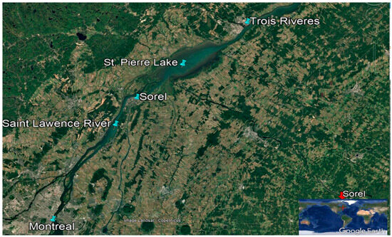
Figure 1.
ECCC observation site at Sorel, Quebec, Canada located at 46.04°N, 73.11°W. The map is derived from Google Earth.
The meteorological instruments were deployed in an open park area, as depicted in Figure 2, which shows views towards the east (Figure 2a) and south (Figure 2b). Towards the east (Figure 2a), there are nearby houses extending southeastwards (not shown in the picture), potentially influencing local sheltering effects. Conversely, the western and southwestern directions (Figure 2b) are relatively open, with scattered trees further away. The instruments are enclosed within an octagonal fence to minimize the wind-induced loss of falling snow. Data for this study were collected using several instruments as follows: the Biral/Metek 24 GHz (K-band) MRR [30] the Vaisala FD71P present weather sensor [31], the OTT PARSIVEL disdrometer, and a single Alter-shielded (SAS) OTT Pluvio2 gauge version 200 with 1500 mm capacity. The SAS OTT Pluvio2 gauge measures P accumulation at 1 min intervals [32]. For winter measurements, the orifice of the Pluvio2 was heated and anti-freeze was also added to melt snow in the collector, but oil was not added to prevent evaporation and this may have impacted the measurements. We have used the proprietary OTT processor firmware (version 1.31) processed data. The Vaisala FD71P sensor provides measurements of the P, PT, and visibility averaged at 1 min intervals, with output recorded every 5 s. It also includes temperature and humidity sensors for RH and T measurements based on the Vaisala HMP155 sensor. The OTT PARSIVEL disdrometer [32,33,34]; measures P, PT, V, and particle size distributions, N(D)s, of precipitation at a 1 min resolution. Detailed descriptions of the FD71P sensor are given in Appendix A. The derivation of N(D) (counts in each size bins), N(D) (), the mean weighted diameter (, the liquid water content (LWC), and the modification of PARSIVEL data for deriving solid-phase precipitation () by including the riming effect in the snowflake density size relationship [35,36,37,38] are also provided in Appendix A. Further details about the Pluvio2, WXT520, and MRR instruments can be found elsewhere [25,30,32]. Vaisala WXT520 measures temperature (T), relative humidity (RH), and wind speed (. In this paper, we only used the data. The MRR provides the vertical profiles of V, LWC, and radar reflectivity () [30]. There have also been occasional radiosonde-based profiling measurements at the same location (46.03°N, 73.11°W). Table 1 summarizes the accuracy, range, and resolution of instrument measurements based on manufacturer specifications. Additionally, intermittent manual snowfall measurements were collected using a snowtube, as part of research conducted by Université du Québec à Montréal (UQAM) [39]. These datasets were used to validate the snowfall measurements from the instruments. Human observations of precipitation type (PT) were also recorded manually every 10 min throughout the project, serving as validation data for instrument-derived PTs. Precipitation comparisons were based on 10 min average datasets, focusing only on dates with recorded precipitation events (see Figure 3).
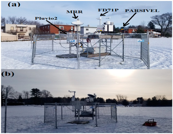
Figure 2.
ECCC instrumentation platform at the Sorel site. Views towards the east (a) and south (b).

Table 1.
Descriptions of the instruments and related relevant information.
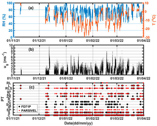
Figure 3.
Observation of T and RH (a), wind speed (WXT520) (b), and precipitation type (PT) based on the FD71P and PARSIVEL (c). In panel (c), the symbols represent no precipitation (C), snow (S), snow pellets (SPs), ice pellets (IPs), snow grains (SGs), ice crystals (ICs), rain (R), freezing rain (ZR), freezing drizzle (ZL), PT is not identified (un), and R+L+S (RLS).
3. Results
3.1. Meteorological Conditions of the Site During the WINTRE-MIX Project
One-minute averaged T, RH, and 2 m height , observed during precipitation events within the measurement period (November 2021–March 2022) at the Sorel site, are given in Figure 3. Temperature varied substantially from −30 °C to 10 °C, with a mean and standard deviation (SD) of −7.7 °C and 12.1 °C, respectively (Figure 3a). The RH varied from 40% to 100% with a mean value of 74% and a SD of 15%, respectively. The wind speed inside the fence, however, did not vary much, only occasionally reaching 10 m s−1, which can be considered mostly calm (Figure 3b). The mean and SD values were 1.42 m s−1 and 1.32 m s−1 respectively. The PT reported based on the FD71P and PARSIVEL shows a variety of precipitation types including ZR, ZL, IP, ice crystals (ICs), snow grains (SGs), snow pellets (SPs), snow (S), rain (R), drizzle (L), R+L+S (RLS), and R+L (RL), where un and C represent the unknown type and non-precipitation condition, respectively (Figure 3c). Note here that the FD71P does not report SPs and the PARSIVEL does not report SGs, ICs, and IPs. Based on visual inspection, the probes were in agreement in detecting C, S, ZR, L, and R events. It is also possible that PARSIVEL may report IPs as SPs. This will be discussed in more detail in Section 3.2.
3.2. PT Manual and Instrument Comparisons
As discussed earlier, there were limited manual observations of PT for a total of 11 days of data, collected every 10 min during precipitation events. Human observations were reported as primary and secondary, according to the occurrence of the most frequent and the least frequent PTs, respectively. In this analysis, only the primary PTs are included for the validation of PT reports based on the instruments.
Figure 4 shows the frequency distribution of PTs for the selected dates that precipitation occurred based on FD71P, PARSIVEL, and manual measurements. The percentage of the PTs detected during these measurement period are given in Table 2. According to these results, both instruments agreed with the manual observation, detecting no precipitation cases (C) (~15%) as compared to the manual detection of 14%, which is slightly lower. This may be attributed to the higher sensitivity of the instruments as compared to the human observer. The manual detection of S (46%) represents a larger fraction of PT events, and it is slightly underestimated by the instruments, FD71P (42.3%) and PARSIVEL (43%). The next significant PT that was manually reported was IPs (12.6%), but this was significantly underdetected by FD71P (2%). PARSIVEL does not report IPs (NA). The next significant PTs manually reported were R (9%), ZR (6%), L (6.3%), and ZL (4%), and when compared to the instruments, FD71P overestimated R (13%) and ZR (18%), underestimated L (1.3%), but agreed very well in detecting ZL (4%). The PARSIVEL probe is somewhat close to the manual observation, as compared to the FD71P probe detecting R (7%), ZR (12%), and L (3.3%), but it detected lower ZL (2%) and higher ZR as compared to the manual observation. There were no significant manual reports for ICs (0%) and SGs (0.7%), which is mostly in agreement with the instruments. Although the datasets were limited, the results suggest that the two instruments were capable of detecting C and S events with reasonable accuracy. The FD71P appears to overestimate ZR and underestimate IPs. Comparing the manual observation taken every 10 min and the interpolated nearest of the manual observation time against the higher resolution data collected every minute by the instruments, some uncertainties were observed, since the instrument-based PT under some conditions fluctuates rapidly within a 10 min interval. More rigorous testing of these instruments using much larger datasets is required to better understand the differences reflected in this study. The other reason could be linked to the instrument algorithm used to diagnose PT, and the possible reasons related to this will be investigated in more detail in Section 3.5.
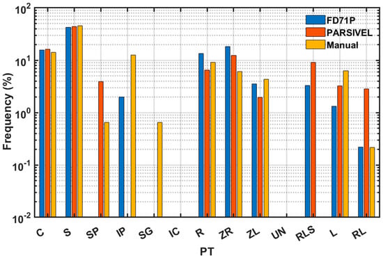
Figure 4.
Frequency distributions of PT reported based on FD71 and PARSIVEL compared to the manual-based observations. The symbols represent no precipitation (C), snow (S), snow pellets (SPs), ice pellets (IPs), snow grains (SGs), ice crystals (ICs), rain (R), freezing rain (ZR), freezing drizzle (ZL), PT is not identified (UN), and R+L+S (RLS).
Table 2.
Frequency distributions of PT based on manual observation and the FD71P and PARSIVEL probes (Figure 4).
3.3. Case Study of Mixed Precipitation on 6 March 20022
Figure 5 shows the time series on 6 March 2022 of PT based on human observation and that reported by the instruments (FD71P and PARSIVEL) (Figure 5a), RH and T (Figure 5b), the number-weighted mean particle velocity (), the diameter () calculated using the PARSIVEL Disdrometer (Figure 5c), and particle spectra (n(D) (Figure 5d). Human observations were made every 10 min and the instruments report PT every min. The human observer reported both the dominant or primary (Man-Prim) PTs and those that are minor or secondary (Man-sec) PTs. Both instruments have reported snow between 4 UTC and 6 UTC (Figure 5a). During this time, the observed T and RH were near −5 and 90%, and they were characterized by relatively enhanced precipitation intensity. The calculated varied from 1mm to 2 mm, and the values of varied from 1 to 1.5 . The maximum diameter of the particle spectra was close to 10 mm, but the majority of the precipitation particles were less than 2 mm in size (Figure 5d), indicating the existence of mostly relatively smaller ice particles, as diagnosed by both the manual observations and present weather sensors (Figure 5c). After 06:00 UTC, the surface temperature started to warm up slightly, and although the remained approximately near 1 mm, the exhibited fluctuations from 1 to about 3 between 6 UTC and 9 UTC under light precipitation, indicating a mixture of particles. The human observation mainly indicated snow with some secondary SPs and SGs near 8 UTC. The PARSIVEL probe also reported mainly snow with some minor SP, which is consistent with human observation, but it occasionally reported ZR and ZL, which are not supported by human observation. In this period, FD71P reported mainly snow, which is consistent with the human observation, with an occasional IP, where the manual observation indicated SP, suggesting that FD71P may have misclassified SPs as IPs. Also, note that between 8 UTC and 9 UTC, the human observer reported mainly IPs with some minor secondary PTs of SPs when FD71P reported mainly snow and some ZR, ZL, and RLS. The human observers did not report RLS, but according to human observation, there was mainly IP, with some secondary SP particles, but FD71P reported these as ZR and snow, which is not consistent with human observation. Between 9 UTC and 11 UTC and between 13 UTC and 16 UTC, both the human observer and the instruments reported ZR, as the surface temperature increased from −3 °C to −1 °C and the RH was close to 90%.
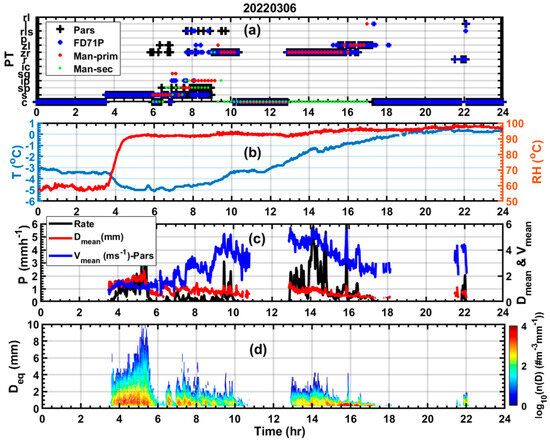
Figure 5.
Time series of human- and instrument-based PT (a); RH and T (b); precipitation intensity (Rate) based on FD71P (P), the mean particle () size and fall velocity () (c); and precipitation particle spectra based on the PARSIVEL disdrometer (d).
Figure 6 shows the time series of the vertical profiles of LWC (Figure 6a), the radar reflectivity factor (Figure 6b), fall velocity (Figure 6c), and surface observation similar to Figure 5d. As indicated in the figure, all ZR events mentioned earlier are associated with ML, as depicted by the enhanced LWC, V, and Ze near 2 km and 2.5 km.
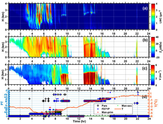
Figure 6.
Time series of liquid water content (LWC) (a), equivalent radar reflectivity factor ( (b), and fall velocity () (c) based on MRR. Time series of the human- and instrument-based precipitation type (PT) (d).
The temperature and RH profiles obtained at 14:40 UTC using a radiosonde (Figure 7a,b) show a freezing level (FL) near 2.5 km that coincides with the data shown in Figure 6b,c. Below the FL, the temperature warmed significantly, close to 5 °C, which could potentially melt the snow. The bottom cold layer (H < 0.5 km) cooled to −2.5 °C, but the surface temperature warmed up, close to −1 °C, because of this and the shallowness of the layer (H < 0.5 km), melted liquid drops remained liquid in a supercooled state when they reached the surface, leading to ZR. The RH profiles show near saturation between heights (0.5 km < H < 4 km) but sub-saturation in the supercooled layer (H < 0.5 km). The ZL events reported after 16:00 UTC do not seem to be associated with any ML, which implies that they are formed via the non-classical freezing mechanism; this cannot be tested because of the absence of radiosonde data.
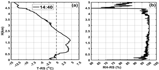
Figure 7.
Vertical profiles of (T) (a) and RH (b), observed using a radiosonde in March.
3.4. Case Study of Mixed Precipitation Dominated by IPs on 23 February 2022
Figure 8 shows similar plots as Figure 5, but in this case, on 23 February 2022, during the period (time < 04:00 UTC), the PT is dominated by IPs according to the human observer, though FD71P reported ZR and the PARSIVEL probe mainly reported RLS (Figure 8a). During the time 04:00-06:30 UTC, both instruments and the human observer reported ZR and ZL, but the human observer reported more frequent ZL. The size distribution also suggests the presence of ZL size particles (D < 0.5 mm) during relatively light precipitation (P < 1 mm h−1), particularly near 03:40 UTC (Figure 8c). During IP events, the surface temperature varied from −7 °C to about −3 °C, which is much colder as compared the first case, but the RH remained close to 90%, and the precipitation intensity varied from 1 mm h−1 to 5 mm h−1. The mean diameter varied slightly from 1 mm to 1.3 mm, and the associated mean velocity varied from 3.5 m s−1 mm to 5 m s−1 (Figure 8c). Most of the particles were below 1.5 mm, reaching a maximum of about 3.5 mm (Figure 8d). During ZR and ZL events, the temperature and RH remained, for the most part, close to −3 °C and 90%, respectively, although the temperature slightly decreased. The possible reasons for some of these discrepancies between the manual and instrument-based PT will be discussed in more depth in Section 3.5.
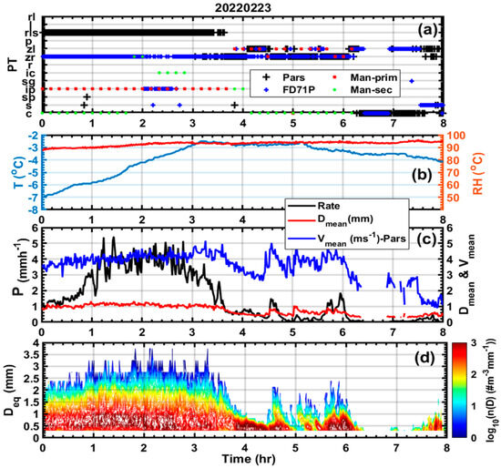
Figure 8.
Time series of human- and instrument-based PT (a); RH and T (b); precipitation intensity (Rate) based on FD71P (P), the mean particle () size and fall velocity () (c); and precipitation particle spectra based on the PARSIVEL disdrometer (d) for 22 February 2022.
As illustrated in Figure 9a–c, all IP events were associated with ML, similar to the ZR case as expected. FL coincided well with the beginning of enhanced fall velocity, LWC, and the radar reflectivity factor, except near 4 UTC where the instruments reported ZR and the human observer reported minor IPs and one event of ZL associated with light precipitation (P < 1 mm h−1).
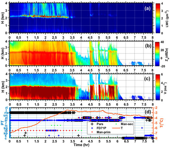
Figure 9.
Time series of liquid water content (LWC) (a), equivalent radar reflectivity factor () (b), and fall velocity (V) (c) based on MRR. Time series of the human- and instrument-based precipitation type (PT) (d) for 23 February 2022.
Figure 10 presents an example of the radiosonde-based vertical profiles of temperature and relative humidity (RH), recorded at 02:00 UTC. As shown in the figure, RH and temperature profiles resemble those observed in the ZR case. However, the freezing level (FL) is comparatively lower (H ≈ 2 km), the bottom cold layer (below 0.5 km) is significantly colder (−7 °C to 0 °C), and the surface temperature is around −5 °C. These conditions contributed to the freezing of supercooled droplets, resulting in IPs.
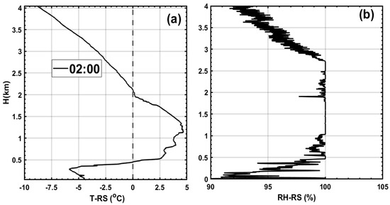
Figure 10.
Vertical profiles of (T) (a) and RH (b), observed using a radiosonde for 23 February 2022, case. (46.03°N, 73.11°W).
3.5. Velocity, Size Relationships, and Precipitation Types
As mentioned earlier, instruments sometimes misclassify some of the PTs because of the similarity in the velocity and size characteristics of the PTs. This is particularly true for the instruments that use the observed V, size (D), and T information to diagnose PT. To investigate these V and D relationships for selected R, ZR, and IP, mixed snow events are investigated. For these comparisons, well-established empirical V-D relationships for rain [40] given as
a theoretically derived V for solid precipitation, proposed by [41] and other relationships based on the observation for fresh hailstones [42] medium density lump graupel [43] and hailstones ([44] have been used (see Table 3).
Table 3.
D in mm and V is in m s−1.
Following [41] (HW), the theoretical derivation of V based on the drag force (), drag coefficient (), falling particle projected area (A), and air density is given as
The authors [41] developed a parameterization that relates to the Reynolds number () in the form
where and . Then, is defined as
where the modified best number (X) is defined as
where is the gravitational acceleration set at 9.8 ms−2, µ is dynamic viscosity of air, is the mass of falling particle, and is the area ratio defined as . Assuming a particle is spherical, the mass of the falling particle, with density , can be estimated as
The terminal velocity or, in this case, the fall velocity is defined as
For this study, fall velocities based on the theoretical approach are calculated using Equation (7), assuming the following parameters hold: = 1.246 kg m−3, = 1.778 × 10⁻⁵ kg (ms)−1, and . The density of a dense solid sphere, such as IP, is assumed to be 0.91 g cm−3 (Ssp = 0.91), while for a fresh, relatively less dense sphere, the density is assumed to be 0.35 g cm−3 (Ssp = 0.35).
Figure 11 shows the observed velocity and size distribution () using the PARSIVEL probe for selected days on 6 March (Figure 11a,b), 17 February (Figure 11c,f), and 23 February (Figure 11d,e), as indicated on the plots during ZR, S, R, and IP events, respectively. The uncertainties in measured fall velocities are removed when V is greater than + 0.5 and lower than − 0.5 for liquid and frozen drop events following [45] and for the case of snow, only particles that exceeded the threshold are removed when they are encountered. The and the ± standard deviation (±SD) of the fall velocity are also given in the plot.
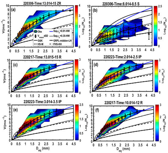
Figure 11.
Velocity and size relationship particle distribution (); mean and ± standard deviation (±SD); empirical velocity and size relationship based on [40] (G&K) for rain, hail stone (HS) based on [44] (HS-M); solid sphere density of snow () 0.91 g cm−3 (Ssp = 0.91) and 0.35 g cm−3 (Ssp = 0.35) based on [41] (HW); lump graupel of medium density based on [43] (GRL-midden-LH); and fresh hailstone [42] (HS-KH)). The dates, times, and observed precipitation types are also displayed. The precipitation types are represented as freezing rain (ZR) (a), snow (S) (b), ice pellets (IP) (d,e), and rain (R) (c,f).
According to the results given in Figure 11, for both during R and ZR events, the closely followed Equation (1) or the empirical curve (Figure 11a–f). However, during IP (Figure 11 d, e) events, the curve line was slightly below the and approximately followed HW, which is consistent with frozen spherical drops (IP) (Figure 11d). This is consistent with previous studies [27,28]. The similarity of the IP and ZR curves suggests that instruments that employ the V-D relationship may sometimes confuse the two, as discussed earlier. In the time interval of Figure 11d (02:00–02:30 UTC), both the manual observation and FD71P were in good agreement (Figure 8a). Even when the two did not agree (Figure 8 and Figure 11e), the results did not change, suggesting that the problem may be related to the type of algorithm being used by the FD71P to differentiate between IPs and ZR/R. On the other hand, in the case shown in Figure 6a, both the human observer and the instruments generally agreed reasonably well, reporting ZR, ZL, and S, except near 08:00 UTC (Figure 5a and Figure 11b). During this time, the human observer reported IPs with some secondary SP, which agreed with PARSIVEL, but the FD71P probe mainly reported S since the FD71P does not normally report SPs. According to the results shown in Figure 11b, the approximately follows the fresh hailstone (FHS-KH) and also the curve that delineates the solid sphere with a density of 0.35 g cm−3 (-HW), particularly at higher values. Thus, this suggests that the presence of mainly nearly spherical particles with a relatively lower density than solid ice, such as SP, sometimes referred to as soft hail, and this is not normally reported by the FD71P.
These results suggest that when PT is dominated by IP, under some conditions, FD71P may misclassify PT as ZR, and this needs to be further investigated to better understand the pertinent reasons. This requires knowing how the Vaisala FD71P diagnosis precipitation type using a proprietary software that is not currently described in its user manual.
3.6. Solid and Freezing Precipitation as a Function of RH and T
As discussed earlier, the precipitation at the surface is determined through dynamical and cloud microphysical process aloft. Traditionally, however, it is the surface temperature that is used to distinguish the boundary between snow and rain and the potential for freezing precipitation. Some recent studies, including the analysis conducted in this study, show that there is a significant variation in the temperature threshold that delineates the snow–liquid boundary [46]. According to [46] the continental climate showed the warmest snow–liquid boundary temperature threshold as compared to maritime climate. The drier (low RH) regions experience more snowfall at relatively warmer temperatures. This has been attributed to the fact that as the solid particles pass through subsaturated environment, the evaporative cooling of the air keeps the falling particles in a solid phase [47] and hence allows solid particles to reach the ground, even at warmer surface temperatures. As a result, some surface models include RH, in addition to T [46,48]. Nonetheless, forecasting the precipitation phase and the associated boundary, between liquid and solid phases is still a challenging problem.
To understand the dependence of precipitation on both surface T and RH, the 2D histogram plots of 1 min averaged freezing precipitation (ZP) and solid precipitation (S, IP, IC, and SG) events are shown in Figure 12. For a similar T range, the ZP events generally occur at a relatively higher RH (RH > 75%), as compared to the solid phase case that shows significant snow events down to RH 50%. During ZP events, the frequency of the occurrence of the event generally increases with an increase in T within the T interval (−10 °C < T < 0 °C), but at warmer temperatures (0 °C < T < 2.5 °C), the frequency becomes rather smaller (Figure 12a), with no significant RH dependence, particularly for T (T > −5 °C). The maximum ZP occurred at a sub-saturated environment (90% < RH < 95%) when the temperatures were warmer (0 °C < T < −5 °C). During solid precipitation events, for a given T, the frequency increased with an increase in RH, but the maximum occurred at relatively lower RH values (80% < RH < 85%) and warmer temperatures, similar to ZP events. For lower RH values (RH < 85%), the occurrence of snow events is more frequent than ZP at warmer temperatures (0 °C < T < 2.5 °C) (Figure 12a,b), confirming the fact that snow events may be more frequent at low RH and warmer temperatures. The inclusion of RH to identify the solid and liquid boundary for some mixed-phase precipitation events may be relevant, but based on this study, it is not straightforward how RH should be incorporated.
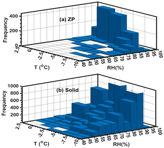
Figure 12.
Composite two-dimensional histograms. 2D density plots of 1 min averaged ZP (a), and solid precipitation (S, IP, IC, and SG) (b) events plotted against T and RH.
Knowing the number of solid- and liquid-phase events at a given temperature interval is possible, however, to derive the percentage of the time that liquid-phase events occurred as a function of the mean temperature and the result is given in Figure 13. According to the results indicated in the plot, on average, at freezing temperature (T = 0 °C), about 60% of the precipitation is in liquid phase. This is remarkably similar to the findings reported in [25] who have used direct manual measurements of liquid and solid precipitation during mixed precipitation events. Complete liquid-phase precipitation does not occur unless the temperature is close to 2 °C. According to this study, the precipitation is not completely solid until the temperature is below −10 °C. In some studies, T = −2 °C was used as a threshold for delineating the upper bound below which the precipitation is completely in a solid phase (e.g., [49]), but as demonstrated here, on average, about 28% of the precipitation could be in liquid phase at this temperature threshold. It should be noted that there are some uncertainties related to the identification of the precipitation type. However, as demonstrated earlier, optical instruments are much more reliable in identifying solid and liquid phases, as compared to the identification of more detailed precipitation types. The results shown in Figure 13 can only be considered in the average sense; it is possible that under some conditions, completely solid-phase precipitation could be observed at temperature (T < −2 °C).
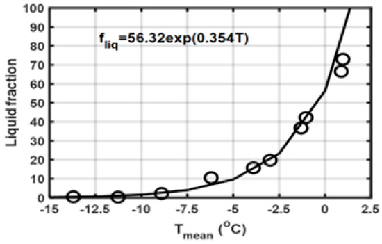
Figure 13.
Liquid fraction calculated based on the observed temperature intervals and precipitation type.
3.7. Precipitation
3.7.1. Comparisons of Solid Precipitation Using the Instruments and Manual Measurements
Validating measured precipitation is challenging without a standard reference, such as a snow gauge, within the Double-Fence Automated Reference [32]. However, sporadic snow depth and snow water equivalent (SWE) measurements were taken using the Snowmetrics Tube Sampler (STS) and a hanging spring scale with a 0.1 mm precision [33]. These measurements were conducted on a 41 cm × 41 cm × 1.25 cm white wooden snowboard. Snow depth was determined as the average of at least three readings, while SWE was based on a single measurement by the UQAM research team. The snowboard was generally cleared before measurements, though occasional lapses were recorded in the dataset. Some uncertainties exist with regard to the measurement process, particularly singular SWE readings, which are likely more prone to error.
Table 4 presents a comparison of measurements taken on four dates in February and March 2022, along with the maximum surface wind speed () at gauge height, temperature (T), and precipitation type (PT). The recorded values were low, minimizing any impact on the collection efficiency of the Pluvio2 gauge or the PARSIVEL probe, which typically respond to increased wind speeds [32]. As shown in the table, some variability exists among the instruments and manual measurements, likely due to uncertainties in the manual methods and differences between instrument techniques. On average, the Pluvio2 gauge recorded lower precipitation amounts compared to manual measurements, while the unmodified PARSIVEL (see Appendix A) reported slightly higher values. Given the low wind speeds ( < 1.5 m s−1), these differences cannot be attributed to wind effects. Notably, the FD71P and modified PARSIVEL data aligned more closely with the manual measurements. A broader analysis of the full dataset reveals similar trends, which will be explored in the following section.
Table 4.
Comparisons of the solid precipitation measurements using FD1P, PARSIVEL, Pluvio2, and manual snow water equivalent (SWE) measurements.
3.7.2. Comparisons of the Instruments Measuring Precipitation Using the Entire Data
Figure 14 presents the 10 min averaged liquid-phase precipitation intensity measured by three different instruments. The plot also includes the correlation coefficient (R) and p-value (), which assess the statistical significance of the results. Typically, values of ≤ 0. 05 are considered significant. As shown, the Pluvio2 gauge (Pluv2) exhibits a reasonable correlation with the optical probes (R = 0.8, ≈ 0; Figure 14a,b). However, considerable scatter is observed at lower intensities (P < 1 mm h−1), likely due to the limited sensitivity of the Pluvio2 gauge [25]. Mean ratio (MR) calculations indicate that the FD71P closely matches the Pluvio2 gauge, with MR = 0.95, whereas the PARSIVEL probe records 45% more precipitation (MR = 1.45). There is no significant difference between PARSIVEL’s calculated measurements using the raw data and directly output precipitation intensities compared to FD71P (Figure 14c,d). The discrepancy between the Pluvio2 gauge and the optical probes may stem from differences in instrument sensitivity. FD71P and PARSIVEL show strong agreement (R = 0.9, ≈ 0), though PARSIVEL measures, on average, 50% more precipitation than FD71P. Since FD71P is a relatively new instrument, further investigation is needed for a definitive assessment.
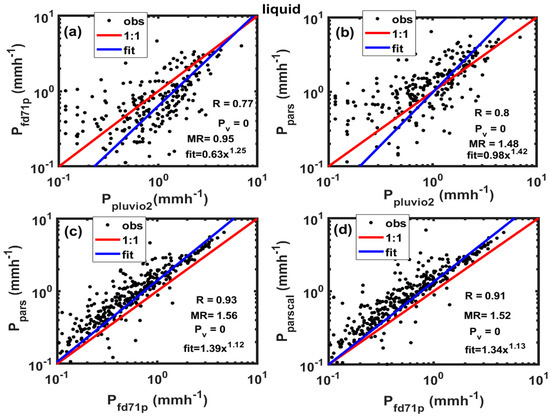
Figure 14.
Liquid precipitation intensity measured using FD71P and Pluvio2 (a), PARSIVEL and Pluvio2 (b), PARSIVEL and FD71P (c), and calculated PARSIVEL ( and FD71P (d). The best fit lines, equations, and statistical p values ( are also given.
As shown in Figure 15a,b, unlike the liquid-phase precipitation in Figure 12, the Pluvio2 gauge underestimates solid-phase precipitation by a factor of two compared to both optical instruments, consistent with findings from the previous section. Given that the 10 min averaged wind speed rarely exceeded 3 m s−1, wind-induced undercatch is unlikely to be the cause. The underestimation may stem from several factors, including the gauge’s lower efficiency in capturing light precipitation compared to optical probes [25]. Additionally, the absence of oil to prevent evaporation could have contributed to this discrepancy. There is also speculation that the heating applied to the gauge’s orifice might generate updrafts, potentially preventing snow particles from entering. Further investigation under controlled conditions is needed to validate this hypothesis. The two optical probes correlate well (R = 0.8), though the unmodified PARSIVEL probe overestimates precipitation by 20% relative to FD71P. However, the modified PARSIVEL probe data, by including the riming effect (Appendix A), aligns closely with that of FD71P (MR = 1; Figure 15d), as also observed in comparisons with manual measurements. The more significant overestimation of precipitation by the unmodified PARSIVEL probe, compared to the Pluvio2 gauge, may be partially attributed to the internal algorithm used by PARSIVEL, particularly in relation to snow density and riming effects. While the PARSIVEL disdrometer has been evaluated using robust standard reference data [32], FD71P is a relatively new instrument and has not undergone similar testing. Further studies are necessary to gain deeper insights into its performance.
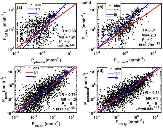
Figure 15.
Solid precipitation intensity measured using FD71P and Pluvio2 (a), PARSIVEL and Pluvio2 (b), PARSIVEL and FD71P (c), and modified PARSIVEL ( and FD71P (d). The best fit lines, equations, and statistical p values ( are also given.
3.7.3. Frequency Distributions of Freezing Precipitation as a Function of and T
Figure 16 shows the 2D frequency distributions of precipitation intensity (P), and T function for ZR and ZL events using the entire datasets shown in Figure 3. Most of freezing precipitation during ZR events occurred during temperature interval (−2.5 °C < T < 0 °C), P < 1 mm h−1, and 0.5 mm < < 1 mm (Figure 16a,b). The maximum P and values during the ZR events reached 5 mm h−1 and 2.5 mm, respectively. On the other hand, most ZL events occurred at colder temperature (−10 °C < T < −2.5 °C), which suggests non-classical formation mechanism [24], mostly associated with P < 0.25 mm h−1. Contrary to ZR events, no ZL events were observed at warmer temperatures (T < 0 °C). The majority of the of the ZL particles ranged between 0.3 < < 0.4 mm. The maximum values of P and during ZL events were 1 mm h−1 and 0.5 mm, respectively. However, most of the larger particles for ZR and ZL events occurred at warmer temperatures (−2.5 °C < T < 0 °C).
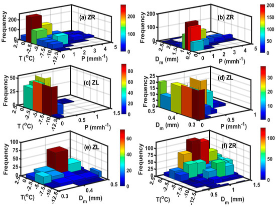
Figure 16.
2D frequency distribution of ZR and ZL as a function temperature and precipitation intensity (P) (a,c), P and (b,d), and temperature and (e,f).
3.7.4. 2D Frequency Distributions of Freezing Precipitation as a Function of and T
Figure 17 shows the LWC calculated (see Appendix A) during freezing precipitation (ZR and ZL), which reached up to 0.6 g m−3, but during most of the events, the LWC was less than 0.1 g m−3 and mostly occurred at temperatures (0 < T < −2.5 °C). There is however a secondary peak in LWC near −7.5 °C, which may be associated with ZL, as indicated in Figure 17. It is also evident that some LWC (<0.1 g m−3) in ZP may occur at warmer temperatures (0 °C < T < 2.5 °C), as would be expected based on Figure 16.
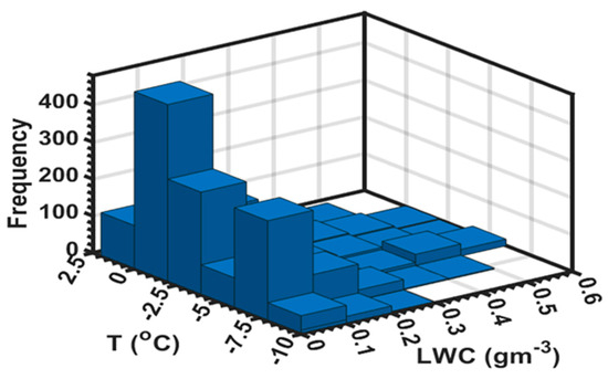
Figure 17.
2D frequency distribution of T and LWC in freezing precipitation.
3.7.5. Relationship Between LWC, , and Freezing Precipitation
The intensity of the icing because of ZP depends on the precipitation intensity and duration of the precipitation. Some empirical models that estimate the ice accretion of the ice thickness use the LWC as input, and this is normally derived using P [50,51,52], based on the empirical power law relationships [53,54]. To compare these power law relationships between LWC and P, 10 min averaged LWC and P were derived based on particle spectra measured using the PARSIVEL probe (Figure 18a). Also, LWC was parameterized as function P and (Figure 18b). The best fit equations are given by Equations (8) and (9).
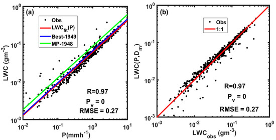
Figure 18.
Ten-minute averaged observed LWC plotted against the precipitation intensity during ZR events (a). Best fit lines based on [53] (Best-1949), [54] (MP-1948), in this study (LWCfit(P)) and the statistical p values ( are also shown. LWC, parameterized as a function of precipitation () and the mean mass-weighted diameter (, plotted against the observed LWC () (b).
According to these results, LWC is strongly correlated with P with a correlation coefficient (R = 0.97, ) and with a root mean square error (RMSE) of 0.27 g m−3. The best fit line agreed well with the one based on [53]. The Marshal and Palmer method slightly overestimates the LWC, and this has also been observed in an earlier study [50]. The inclusion of did not improve the estimation of the LWC, but parameterization may be used to derive using the two equations since it is one of the most important parameters used for the parameterization of particle size distribution (e.g., [55,56]).
4. Conclusions
In this study, we have analyzed data collected in wintertime mixed-phase precipitation using several specialized instruments, including the Vaisala FD71P and PARSIVEL probes that measure precipitation, type (P), fall velocity (V), and precipitation size spectra (N(D)). We also used a Micro Rain Radar (MRR) that measures V and radar reflectivity () and a single Alter-shielded Pluvio2 that measures precipitation (P). The data includes some manual measurements of PT and the snow water equivalent (SWE) snowfall based on the Snowmetrics Tube Sampler. The observed P and PT measured using the FD71P and PARSIVEL probes were compared against the manual measurements, as well as the Pluvio2 precipitation gauge. The P and PT were characterized based on temperature (T) and humidity (RH), and microphysical quantities such as the mean mass-weighted diameter (), fall velocity (V), and liquid water content (LWC). Freezing precipitation (ZP) and solid precipitation events were studied using integrated datasets of surface-based observations and vertical profiling data obtained using the MRR and radiosonde. Based on this study, the following key findings have been noted:
The comparison of the reported PT against human observation shows that FD71P and PARSIVEL agree reasonably well in detecting liquid-phase precipitation and snow events. However, the FD71P significantly overestimates freezing rain (ZR) and underestimates ice pellet (IP) events. Generally, the PARSIVEL detected rain (R), ZR, and snow (S) better than the FD71P. The FD71P was better at detecting ZL, and only the FD71P could detect IPs. The discrepancy may relate to the uncertainty of the V-D relationship used for diagnosing ZR and IPs. More studies are needed to draw definite conclusions due to the limited manual datasets.
Further analysis of the PARSIVEL data showed similar V-D relationships during IP and ZR events. However, the V-D curve was slightly lower than the empirical liquid-phase curve. The V for IPs can be theoretically modeled assuming frozen spherical drops, which is consistent with previous studies.
The integrated vertical profiling data from the MRR and radiosonde, and the surface observations during ZR and IP events, show both events are associated with ML. The warm layer depth was 2 km, and the RH was near saturation, but the surface temperature during IP events was much colder. This suggests that surface temperature is a controlling factor determining IPs or ZR.
Statistical 2D histograms of ZR and ZL events under different surface environmental conditions showed that most of the ZR events occurred at warmer temperatures as compared to ZL events that mostly occurred at colder temperatures. Most of the P and associated with ZR and ZL were (P < 1 mm h−1 and < 1 mm) and (P < 0.25 mm h−1 and < 0.4 mm), respectively. The majority of the larger particles, however, occurred at relatively warmer temperatures for both events. The 2D histogram of LWC and T during ZP (ZR + ZL) events resembles the 2D histogram of P and T, showing two distinct peaks, one for ZR at warmer temperatures and the other for ZL at colder temperatures. The more frequent LWC values observed for both ZR and ZL events were less than 0.1 g m−3, although the value reached up to 0.6 g m−3 under some environmental conditions.
According to this study, there is some evidence that at low RH, more snow events occur than at warmer temperatures (0 °C < T < 2.5 °C), as compared to ZP, but on average, it is T that mostly controls the precipitation phase. A simple calculation of the percentage of the phase fraction based on the measurements of the precipitation phase and temperature reveals that, at freezing temperatures, on average, close to 40% of precipitation is in solid phase, and the total ice phase does not occur until the temperature is close to −10 °C. This is consistent with previous findings [25].
Comparisons of precipitation measured using the optical probes (FD71P and PARSIVEL) and the SAS Pluvio2 gauge showed different results when compared during solid and liquid precipitation events. During the liquid events, although the comparison between Plivio2 and the two optical probes showed reasonable correlation (R = 0.8), there was significant scatter at lower p values (P < 1 mm h−1). The two optical probes were well correlated (R = 0.9), although the PARSIVEL probe, on average, overpredicted precipitation events. During snow events, the Pluvio2 gauge consistently underestimated snowfall events by a factor near to two, even when compared to manual measurements. This underestimation may be attributed to several factors, including the gauge’s reduced efficiency in capturing light precipitation compared to optical probes [25]. Additionally, the lack of oil to prevent evaporation could have further contributed to this discrepancy. There is also speculation that the heating applied to the gauge’s orifice could have created updrafts, potentially obstructing snow particles from entering the gauge. Further investigation under controlled conditions is needed to validate this hypothesis. On the other hand, the two optical probes agreed reasonably well (R = 0.8). The snowfall amounts derived using a modified algorithm that includes riming effects agreed relatively well with the FD71P and manual snow measurements. It should be noted that the manual snow measurements were only limited to a few days, and it is recommended that these instruments, particularly the FD71P, being relatively new, be tested using a standard reference gauge.
The functional relationship between ZP intensity and LWC derived from the PARSIVEL probe showed excellent agreement with [53]. However, the relationship based on [54] N(D) parameterization overestimated LWC, as noted by other researchers (e.g., [50]).
Author Contributions
Conceptualization, methodology, software, validation, formal analysis, investigation, data curation, and writing—original draft preparation, F.S.B.; resources and project administration, D.M.; data curation, R.R. and S.H.; writing—review and editing, M.L., G.A.I. and J.A.M. All authors have read and agreed to the published version of the manuscript.
Funding
This research received no external funding.
Data Availability Statement
The data can be accessed following this link https://data.eol.ucar.edu/master_lists/generated/wintre-mix/.
Acknowledgments
The author would like to acknowledge Robert Crawford for archiving the data.
Conflicts of Interest
Author George A. Isaac was employed by the company Weather Impacts Consulting Incorporated. The remaining authors declare that the research was conducted in the absence of any commercial or financial relationships that could be construed as a potential conflict of interest.
Appendix A
Appendix A.1. Brief Description of the Vaisala FD71P
The FD71P is a relatively new instrument developed by Vaisala, and it is briefly described in their website https://docs.vaisala.com/v/u/B211744EN-G/en-US (accessed on 1 March 2025). According to its user manual and description given in [31], it is a forward-scattering probe like the previous Vaisala present weather sensors with some modification in its forward-scattering geometry. This version also provides particle size and velocity information in addition to precipitation, type, and visibility. It is equipped with a transmitter and a receiver, similar to previous present weather seniors, but in this case, the transmitter and receiver are geometrically configured to look downward, and the transmitter transmits a thin sheet of light at a wavelength (λ = 850 nm), as opposed to the conventional light cone, and the receiver measures the forward scattered light at an angle of 42°. The instrument outputs the precipitation particle number at 41 size and 26 velocity bins. According to the user’s manual, the particle size measured in a range 0.1–7+ mm and velocity in a range 0–10+ m s−1. Unfortunately, no bin sizes are assigned for bins >40, the last 41 bin represents any size greater than 7 mm, this makes it difficult to analyze the particle distribution spectra (D > 7 mm), particularly for snow. According to the manufacturer, the instrument can measure the shape, size, and velocity of the falling hydrometeors, but no descriptions are provided in the user manual on how these are archived. The sampling area of the instrument is 3800 mm2 and the sampling time is 60 s (Vaisala Phillip A. Allegretti personal communication). According to the user manual, the instrument can measure precipitation intensity in the range 0.01–999.99 mm h−1, at a resolution of 0.01 mm, meeting the WMO standard (see Table 1). The look-down geometry and hood heating protect the sensor windows against external disturbances. The FD70 series complies with the ICAO, FAA, and WMO requirements and uses the WMO and NWS weather codes in reporting. It has a visibility up to 100 km and an optimal forward scattering angle of 42 degrees. It has a 5 MHz sampling frequency and a 5 s measuring cycle. The instrument also incorporates a Vaisala HMP155 HUMICAP probe that measures the humidity and temperature of the air (see Table 1).
Appendix A.2. PARSIVEL Data Processing
The PARSIVEL probe measures velocity and size spectra based on 32 size and 32 velocity bins; more details are given elsewhere [25,34]. The particle number per bin size is calculated as
where is the number of particles for each size (i) and velocity (j) bins; D is the volume equivalent diameter in mm. The number concentration in is given as
where is the sampling time set at 60 s, is the sampling area set at 0.0054 m2, is the fall velocity in , and is the bin spread given in mm.
The modified snowfall rate () in mm h−1 was calculated as
where D is in mm, based on [35] and is the degree of riming given as
following [36,37], where is the mean observed fall velocity and is given following [57] as
The modification of snow density using was first introduced by [38]. The liquid-phase precipitation in this paper is also calculated to be compared with one directly output by the PARSIVEL probe using a similar expression, given in Equation (A3), as
where is the density of the water given as 0.001 . The liquid water content (LWC) was calculated as
The mean mass-weighted diameter () in mm is given as
References
- Cortinas, J.V.; Bernstein, B.C.; Robbins, C.C.; Strapp, J.W. An analysis of freezing rain, freezing drizzle, and ice pellets across the United States and Canada: 1976–1990. Weather Forecast. 2004, 19, 377–390. [Google Scholar] [CrossRef]
- Adhikari, A.; Liu, C. Remote sensing properties of freezing rain events from space. J. Geophys. Res. Atmos. 2019, 124, 10385–10400. [Google Scholar] [CrossRef]
- Deng, D.; Gao, S.; Du, X.; Wu, W. A diagnostic study of freezing rain over Guizhou, China, in January 2011. Q. J. R. Meteorol. Soc. 2012, 138, 1233–1244. [Google Scholar] [CrossRef]
- Lott, N.; Ross, D.; Graumann, A.; Eastern, U.S. Flooding and Ice Storm January 1998; Tech. Rep.; NOAA/National Climatic Data Center: Asheville, NC, USA, 1998; p. 6. [Google Scholar]
- De Gaetano, A.T. Climatic perspective and impacts of the 1998 northern New York and New England ice storm. Bull. Am. Meteorol. Soc. 2000, 81, 237–254. [Google Scholar] [CrossRef]
- Gyakum, J.R.; Roebber, P.J. The 1998 ice storm—Analysis of a planetary-scale event. Mon. Weather Rev. 2001, 129, 2983–2997. [Google Scholar] [CrossRef]
- Roebber, P.J.; Gyakum, J.R. Orographic influences on the mesoscale structure of the 1998 ice storm. Mon. Weather Rev. 2003, 131, 27–50. [Google Scholar] [CrossRef]
- Strapp, J.W.; Stuart, R.A.; Isaac, G.A. A Canadian climatology of freezing precipitation and a detailed study using data from St. John’s, Newfoundland. In Proceedings of the FAA International Conferrence on Aircraft Inflight Icing, FAA, DOT/FAA/AR-96/81. Springfield, VA, USA, 6–8 May 1996; Volume 2, pp. 45–56. [Google Scholar]
- Stuart, R.A.; Isaac, G.A. Freezing precipitation in Canada. Atmosphere-Ocean 1999, 37, 87–102. [Google Scholar] [CrossRef][Green Version]
- Boudala, F.S.; Isaac, G.A. Parameterization of visibility in snow: Application in numerical weather prediction models. J. Geophys. Res. 2009, 114, D19202. [Google Scholar] [CrossRef]
- Huffman, G.J.; Norman Jr., G. A. The supercooled warm rain process and the specification of freezing precipitation. Mon. Weather Rev. 1988, 116, 2172–2182. [Google Scholar] [CrossRef]
- Bocchieri, J.R. A new operational system for forecasting precipitation type. Mon. Weather Rev. 1979, 107, 637–649. [Google Scholar] [CrossRef]
- Rauber, R.M.; Olthoff, L.; Ramamurthy, M.; Kunkel, K. The relative importance of warm rain and melting processes in freezing precipitation events. J. Appl. Meteor. 2000, 39, 1185–1195. [Google Scholar] [CrossRef]
- Bernstein, B. Regional and local influences on freezing drizzle freezing rain, and ice pellets. Weather Forecast. 2000, 15, 485–508. [Google Scholar] [CrossRef]
- Hanesiak, J.; Stewart, R. The mesoscale and microscale structure of a severe ice pellet storm. Mon. Weather Rev. 1999, 123, 3144–3162. [Google Scholar] [CrossRef]
- Zerr, R.J. Freezing rain: An observational and theoretical study. J. Appl. Meteor. 1997, 36, 1647–1661. [Google Scholar] [CrossRef]
- Gascón, E.; Hewson, T.; Haiden, T. Improving predictions of precipitation type at the surface: Description and verification of two new products from the ECMWF ensemble. Weather Forecast. 2018, 33, 89–108. [Google Scholar] [CrossRef]
- Ralph, F.M.; Rauber, R.M.; Jewett, B.F.; Kingsmill, D.E.; Pisano, P.; Pugner, P.; Rasmussen, R.M.; Reynolds, D.W.; Schlatter, T.W.; Stewart, R.E.; et al. Improving short-term (0–48 h) cool-season quantitative precipitation forecasting: Recommendations from a USWRP workshop. Bull. Am. Meteorol. Soc. 2005, 86, 1619–1632. [Google Scholar] [CrossRef]
- Tessendorf, S.A.; Ugg, A.; Korolev, A.; Heckman, I.; Weeks, C.; Thompson, G.; Jacobson, D.; Adriaansen, D.; Hagger, J. Differentiating Freezing Drizzle and Freezing Rain in HRRR Model Forecasts. Weather Forecast. 2021, 36, 1237–1251.4. [Google Scholar] [CrossRef]
- Thériault, J.M.; Stewart, R.E.; Henson, W. On the dependence of winter precipitation types on temperature, precipitation rate, and associated features. J. Appl. Meteor. Climatol. 2010, 49, 1429–1442. [Google Scholar] [CrossRef]
- Ikeda, K.; Steiner, M.; Thompson, G. Examination of mixed-phase precipitation forecasts from the High-Resolution Rapid Refresh model using surface observations and sounding data. Weather Forecast. 2017, 32, 949–967. [Google Scholar] [CrossRef]
- Bourgouin, P. A method to determine precipitation types. Weather Forecast. 2000, 15, 583–592. [Google Scholar] [CrossRef]
- Baldwin, M.; Treadon, R.; Contorno, S. Precipitation type prediction using a decision tree approach with NMC’s Meso- scale Eta Model. In Proceedings of the 10th Conference on Numerical Weather Prediction, Portland, OR, USA, 18–22 July 1994; pp. 30–31. [Google Scholar]
- Isaac, G.A.; Cober, S.G.; Korolev, A.V.; Strapp, J.W.; Tremblay, A.; Marcotte, D.L. Overview of the Canadian freezing drizzle experiment I, II, and III. In Proceedings of the Cloud Physics Conference, Everett, WA, USA, 17–21 August 1998. [Google Scholar]
- Boudala, F.S.; Isaac, G.A.; Filman, P.; Crawford, R.; Hudak, D. Performance of Emerging Technologies for Measuring Solid and Liquid Precipitation in Cold Climate as Compared to the Traditional Manual Gauges. J. Atmos. Oceanic Technol. 2017, 34, 167–184. [Google Scholar] [CrossRef]
- Boudala, F.S.; Isaac, G.A.; Wu, D. Aircraft Icing Study Using Integrated Observations and Model Data. Weather Forecast. 2019, 34, 485–506. [Google Scholar] [CrossRef]
- Lachapelle, M.; Thompson, H.D.; Leroux, N.R.; Thériault, J.M. Measuring Ice Pellets and Refrozen Wet Snow Using a Laser-Optical Disdrometer. J. Appl. Meteorol. Climatol. 2024, 63, 65–84. [Google Scholar] [CrossRef]
- Rahman, K.; Testik, F.Y. Shapes and Fall Speeds of Freezing and Frozen Raindrops. J. Hydrometeorol. 2020, 21, 1311–1331. [Google Scholar] [CrossRef]
- Minder, J.R.; Bassill, N.; Fabry, F.; French, J.; Friedrich, K.; Gultepe, I.; Gyakum, J.D.; Kingsmill, K.; Kosiba; Lachapelle, M.; et al. P-Type Processes and Predictability: The Winter Precipitation Type Research Multiscale Experiment (WINTRE-MIX)-BAMS2023. Bull. Am. Meteorol. Soc. 2023, 104, E1469–E1492. [Google Scholar] [CrossRef]
- METEK, Micro Rain Radar (MRR), MRR-2 and MRR-Pro a Tutorial. 2017. Available online: https://metek.de/wp-content/uploads/2016/12/2018-0206-MRR_tutorial.pdf (accessed on 1 March 2025).
- Klugmann, D.; Kauppinen, L. FD70—A Tool for Supporting Satellite Weather Observations. IGARSS. 2022. Available online: https://ieeexplore.ieee.org/stamp/stamp.jsp?tp=&arnumber=9883220 (accessed on 1 March 2025).
- Boudala, F.S.; Milbrandt, J.A. Solid Precipitation and Visibility Measurements at the Centre for Atmospheric Research Experiments in Southern Ontario and Bratt’s Lake in Southern Saskatchewan. Remote Sens. 2023, 15, 4079. [Google Scholar] [CrossRef]
- Boudala, F.S.; Isaac, G.A.; Rasmussen, R.; Cober, S.; Scott, B. Comparisons of snowfall measurements in complex terrain made during the 2010 Winter Olympics in Vancouver. Pure Appl. Geophys. 2014, 171, 113. [Google Scholar] [CrossRef]
- Lofflermang, M.; Joss, J. An optical disdrometer for measuring size and velocity of hydrometeors. J. Atmos. Oceanic Technol. 2000, 17, 130–139. [Google Scholar] [CrossRef]
- Holroyd, E.W., III. The Meso- and Microscale Structure of Great Lakes Snowstorm Bands: A Synthesis of Ground Measurements, Radar Data, and Satellite Observations. Ph.D. Thesis, University at Albany, State University of New York, Albany, NY, USA, 1971; p. 148. [Google Scholar]
- Bukovcic, P.; Ryzhkov, A.; Zrnic´, D.; Zhang, G. Polarimetric radar relations for quantification of snow based on Disdrometer data. J. Appl. Meteor. Climatol. 2018, 57, 103–120. [Google Scholar] [CrossRef]
- Zhang, G. Weather Radar Polarimetry; CRC Press: Boca Raton, FL, USA, 2016; p. 304. [Google Scholar]
- Zawadzki, I.; Szyrmer, W.; Bell, C.; Fabry, F. Modeling of the melting layer. Part III: The density effect. J. Atmos. Sci. 2005, 62, 3705–3723. [Google Scholar] [CrossRef]
- Han, B.; Minder, J.R.; Winters, A.; Baima, R.; Thériault; Lachapelle, M.; Gyakum, J.; Wray, J. WINTRE-MIX: Manual Hydrometeor Observation Reports; Version 1.0.11 Data Files, 2 Ancillary/Documentation Files, KiB; UCAR/NCAR-Earth Observing Laboratory: Boulder, CO, USA, 2022. [Google Scholar] [CrossRef]
- Gunn, R.; Kinzer, G.D. Terminal velocity of water droplets in stagnant air. J. Atmos. Sci. 1949, 6, 243–248. [Google Scholar] [CrossRef]
- Heymsfield, A.J.; Westbrook, C.D. Advances in the estimation of ice particle fall speeds using laboratory and field measurements. J. Atmos. Sci. 2010, 67, 2469–2482. [Google Scholar] [CrossRef]
- Knight, N.C.; Heymsfield, A.J. Measurement and interpretation of hailstone density and terminal velocity. J. Atmos. Sci. 1983, 40, 1510–1516. [Google Scholar] [CrossRef]
- Locatelli, J.D.; Hobbs, P. Fall speeds and masses of solid precipitation particles. J. Geophys. Res. V 1974, 79, 2185–2197. [Google Scholar] [CrossRef]
- Mitchell, D.L. The use of mass- and area-dimensional power laws for determining precipitating particle terminal velocities. J. Atmos. Sci. 1996, 53, 1710–1723. [Google Scholar] [CrossRef]
- Letson, F.; Pryor, S.C. From Hydrometeor Size Distribution Measurements to Projections of Wind Turbine Blade Leading-Edge Erosion. Energies 2023, 16, 3906. [Google Scholar] [CrossRef]
- Jennings, K.S.; Winchell, T.S.; Livneh, B.; Noah, P. Spatial variation of the rain–snow temperature threshold across the Northern Hemisphere. Nat. Commun. 2018, 9, 1148. [Google Scholar] [CrossRef]
- Nagumo, N.; Fujiyoshi, Y. Microphysical properties of slow-falling and fast-falling ice pellets formed by freezing associated with evaporative cooling. Mon. Wea. Rev. 2001, 143, 4376–4392. [Google Scholar] [CrossRef]
- Sun, F.; Chen, Y.; Li, Y.; Li, Z.; Duan, W.; Zhang, Q.; Chuan, W. Incorporating relative humidity improves the accuracy of precipitation. Atmos. Res. 2022, 271, 106094. [Google Scholar] [CrossRef]
- Smith, C.D.; Ross, A.; Kochendorfer, J.; Earle, M.E.; Wolff, M.; Buisán, S.; Roulet, Y.-A.; Laine, T. Evaluation of the WMO Solid Precipitation Intercomparison Experiment (SPICE) transfer functions for adjusting the wind bias in solid precipitation measurements. Hydrol. Earth Syst. Sci. 2020, 24, 4025–4043. [Google Scholar] [CrossRef]
- Jones, K.F. A simple model for freezing rain ice loads. Atmos. Res. 1998, 46, 87–97. [Google Scholar] [CrossRef]
- Jones, K.F. Freezing Fraction in Freezing Rain. Weather Forecast. 2022, 47, 163–178. [Google Scholar] [CrossRef]
- Cao, Y.; Wu, Z.; Xu, Z. Effects of rainfall on aircraft aerodynamics. Prog. Aerosp. Sci. 2014, 71, 85–127. [Google Scholar] [CrossRef]
- Best, A.C. The size distribution of raindrops. Quart. J. Roy. Meteor. Soc. 1949, 76, 16–36. [Google Scholar] [CrossRef]
- Marshall, J.S.; Palmer, W.M. The distribution of raindrops with size. J. Meteorol. 1948, 5, 165–166. [Google Scholar] [CrossRef]
- Testud, J.; Oury, S.; Amayenc, P.; Black, R.A. The concept of ‘‘normalized’’ distributions to describe raindrop spectra: A tool for cloud physics and cloud remote sensing. J. Appl. Meteor. 2001, 40, 1118–1140. [Google Scholar] [CrossRef]
- Bringi, V.N.; Chandrasekar, V.; Hubbert, J.; Gorgucci, E.; Randeu, W.L.; Schoenhuber, M. Raindrop size distribution in different climatic regimes from disdrometer and dualpolarized radar analysis. J. Atmos. Sci. 2003, 60, 354–365. [Google Scholar] [CrossRef]
- Brandes, E.A.; Ikeda, K.; Zhang, G.; Schonhuber, M.; Rasmussen, R.M. A statistical and physical description of hydrometeor distributions in Colorado snowstorms using a video disdrometer. J. Appl. Meteor. Climatol. 2007, 46, 634–650. [Google Scholar] [CrossRef]
Disclaimer/Publisher’s Note: The statements, opinions and data contained in all publications are solely those of the individual author(s) and contributor(s) and not of MDPI and/or the editor(s). MDPI and/or the editor(s) disclaim responsibility for any injury to people or property resulting from any ideas, methods, instructions or products referred to in the content. |
© 2025 by the authors. Licensee MDPI, Basel, Switzerland. This article is an open access article distributed under the terms and conditions of the Creative Commons Attribution (CC BY) license (https://creativecommons.org/licenses/by/4.0/).