Amplitude and Phase Calibration with the Aid of Beacons in Microwave Imaging Radiometry by Aperture Synthesis: Algebraic Aspects and Algorithmic Implications

Abstract

In remote sensing via aperture synthesis, the complex gains of every elementary antenna have to be very well known for measuring accurate complex visibilities. The role of calibration is to estimate the instrumental and environmental variations that may affect interferometric measurements. This contribution focuses on the calibration of the effective transfer function of aperture synthesis radiometers with the aid of a radio beacon, in the same way radio-astronomers use quasi-stellar radio sources to calibrate that of radio-telescope arrays. If the amplitude calibration of complex gains does not raise any issue, it is shown that phase calibration may bring up serious challenges if it is not given special attention. Indeed, the phase of the complex visibilities cannot be roughly unwrapped as the risk of a wrong estimation of the complex gains is real and proven. This problem is overcome with the aid of a non-linear optimization algorithm for iteratively and smoothly unwrapping these phases. The performances of both amplitude and phase calibration are then assessed by means of numerical simulations with emphasis on the sensitivity of the accuracy to the inversion method as well as to various errors.

1. Introduction

Microwave radiometry is a remote sensing technique that aims at measuring the brightness temperature of the Earth’s surface [1]. It is well known that the achievable spatial resolution of such direct measurements is limited by the size of real aperture antennas [2]. This is why synthetic apertures providing interferometric measurements are also used to reach higher spatial resolutions [3]. While classical radiometers measure the power collected by a highly directive antenna, interferometric measurements with an aperture synthesis radiometer are obtained by cross-correlating the signals collected by pairs of non-directive elementary antennas having overlapping fields of view [4]. As a consequence, if total power radiometers provide direct measurements of the brightness temperature in the main beam direction of the antenna, aperture synthesis radiometers require the aid of a computer to invert the so-called complex visibilities [5] and to retrieve the brightness temperature distribution in front of the antenna array [6]. This imaging concept was initially developed for radio astronomy some decades ago [7] and it has been recently used with success for remote sensing of the Earth’s surface in the microwave range with the Soil Moisture and Ocean Salinity [8] (SMOS) space mission.

The accuracy of brightness temperatures measured with real aperture radiometers relies on the quality of calibration techniques (external targets, vicarious sources, and internal calibrators like noise diodes or matched reference loads) [9]. This is the same with synthetic aperture radiometers for which the complex gains of every elementary antenna of the array have to be very well known for measuring accurate complex visibilities. For the Microwave Imaging Radiometer with Aperture Synthesis [10] (MIRAS), the unique payload of SMOS, on-board calibration is accomplished by a dedicated circuitry with the conventional noise distribution technique through a network of cables [11]. However, there exist situations where this standard direct calibration cannot be implemented. This is the case, for example, with the formation of flying interferometric radiometers [12] for which a new approach based on non-directional beacons [13] has been proposed [14], similar to that used for decades in radio astronomy with quasars (Chapter 5 in [15]). It might also be the case for synthetic aperture radiometers without any specific circuitry [16] devoted to this task, for example, to reduce costs, and which therefore also rely on such beacons for this exercise.

As soon as the L-band [17] is concerned, it may be useful to briefly recall some official rules on the usage of the radio spectrum. The frequency band 1400–1427 MHz is protected from any emissions [18] since it is allocated to the Earth exploration-satellite service and to the space research service (both passive), as well as to the radio astronomy service. As a consequence, for any space-borne antenna arrays operating in the L-band, if calibration with the aid of ground-based beacons is visualized, they cannot emit in that protected band. One solution, which has been proposed for the synchronization of the signals maintained by the elementary antennas of the Unconnected L-band Interferometer Demonstrator [19] (ULID), is to use the 1427–1429 MHz service band, the closest band to the protected band 1400–1427 MHz. Indeed, according to the decision of the Electronic Communications Committee [18] (ECC), the band 1427–1429 MHz is a service band allocated to the fixed, mobile and space operation (Earth-to-space) services. It can therefore be used for the calibration of space-borne antenna arrays with ground-based beacons, provided that the beacons respect the ECC decision in terms of emitted power and the antenna arrays are equipped with adequate filters. Finally, with regard to any other practical aspects of such a calibration, particularly on the constraints related to its spatial implementation, more information can be found in the comprehensive study in [14].

The idea of aperture synthesis is to obtain high-angular-resolution images by using interferometric information from pairs of elementary antennas [7]. More precisely, the signals collected by every elementary antenna are combined pair-wise in a complex cross-correlator [20] yielding samples of the coherence function [21], also termed complex visibilities [22], of the brightness temperature distribution of the scene observed by the antenna array [23]. Fundamentally, only the information that cannot be factored into elementary antenna terms, i.e., the information that depends on antenna pairs only, is credible as being of scientific interest because of Earth or sky emission origin. The success of aperture synthesis therefore relies on the ability to calibrate every elementary antenna. As a consequence, calibration is of the utmost importance [24] before addressing synthesis imaging. It deals directly with the interferometric measurements which may be affected by perturbations. Calibration is the effort made for estimating and finally for removing these instrumental and environmental variations that affect the measured complex visibilities. If these perturbations are not reduced or mitigated, they will directly transfer in severe distortions or artifacts [25,26,27] in the retrieved brightness temperature maps obtained when inverting the complex visibilities with the aid of a computer.

The integral relations between the complex visibilities and the distribution of the brightness temperature of a scene observed by an antenna array are described in Section 2. Then, the effective transfer function between the observed visibilities and the expected visibilities is introduced and discussed. Section 3 is devoted to the linear aberration operators involved in solving the calibration equations for retrieving amplitudes and phases of the complex gains of every elementary antenna. For clarity, the corresponding theoretical formulation here is reduced to the strict minimum, but additional details on linear algebra concepts and on the properties of these key operators are relegated in Appendix A. The different calibration techniques that are usually implemented in aperture synthesis are briefly introduced in Section 4. The main purpose here is the calibration plan, or scenario, that is proposed when the approach is based on interferometric information obtained from observations of a non-directional beacon. The algebraic equations to be solved for amplitude and phase calibration are developed and discussed in Section 5. If amplitude calibration does not raise any problem, it is shown that phase calibration has to be addressed with care as it may bring up a serious challenge if the phase is unwrapped roughly. A non-linear optimization algorithm is created to overcome this issue; this is explained in detail in Appendix B. Finally, the performances of both amplitude and phase calibration are assessed in Section 6 by means of numerical simulations with particular attention paid to the sensitivity of the accuracy to the inversion method and to various errors. This comprehensive study is conducted with the antenna array of the FANTASIOR project, a common R&D program of CNES and CESBIO which aims at recording the radio signals maintained by elementary antennas operating in the 1400–1429 MHz frequency band for deferred processing with the idea, among others, to compile them in the protected band 1400–1427 MHz, all together and additively for digital beam forming or by pairs in a multiplicative way for synthetic aperture interferometry [28], while using the service band 1427–1429 MHz for the calibration of the effective transfer function.

2. Theoretical Aspects

According to the van Cittert–Zernike theorem [29,30], the theoretical complex visibility $V_{pq}$ in the far-field approximation is given by the following integral relation:

$${\displaystyle V_{pq}=\underset{\parallel \mathit{\xi }\parallel \le 1}{\int \int } \frac{{\mathcal{F}}_p^{\phantom{*}}\left(\mathit{\xi }\right)}{\sqrt{{\Omega }_p}}\frac{{\mathcal{F}}_q^{*}\left(\mathit{\xi }\right)}{\sqrt{{\Omega }_q}}T\left(\mathit{\xi }\right){\mathrm{e}}^{{\displaystyle {\displaystyle -2\mathrm{j}\pi \frac{{\mathbf{b}}_{pq}·\mathit{\xi }}{{\lambda }_o}}\phantom{\frac{a}{\lambda }}}}\frac{\mathrm{d}\mathit{\xi }}{\sqrt{1-{\parallel \mathit{\xi }\parallel }^2}},}$$

(1)

which has to be substituted by the more general expression as follows:

$${\displaystyle V_{pq}=\underset{ \parallel \mathit{\xi }\parallel \le 1}{\int \int }\frac{{\mathcal{F}}_p^{\phantom{*}}\left({\mathit{\xi }}_p\right)}{\sqrt{{\Omega }_p}}\frac{{\mathcal{F}}_q^{*}\left({\mathit{\xi }}_q\right)}{\sqrt{{\Omega }_q}}T\left(\mathit{\xi }\right)\frac{r^2\left(\mathit{\xi }\right)}{r_p\left(\mathit{\xi }\right)r_q\left(\mathit{\xi }\right)}{\mathrm{e}}^{{\displaystyle {\displaystyle -2\mathrm{j}\pi \frac{r_q\left(\mathit{\xi }\right)-r_p\left(\mathit{\xi }\right)}{{\lambda }_o}}\phantom{\frac{a}{\lambda }}}}\frac{\mathrm{d}\mathit{\xi }}{\sqrt{1-{\parallel \mathit{\xi }\parallel }^2}},}$$

(2)

if near-field conditions have to be taken into account in the modeling, as explained in [31]. In these twin expressions, ${\mathcal{F}}_p$ and ${\mathcal{F}}_q$ are the voltage patterns of the two elementary antennas ${\mathcal{A}}_p$ and ${\mathcal{A}}_q$ with equivalent solid angles ${\Omega }_p$ and ${\Omega }_q$, T is the brightness temperature distribution of the observed scene, and ${\lambda }_o$ is the central wavelength of observation. The two components ${\xi }_1=sin\theta cos\varphi$ and ${\xi }_2=sin\theta sin\varphi$ of the angular position variable $\mathit{\xi }$ are direction cosines ($\theta$ and $\varphi$ are the traditional spherical coordinates) in the reference frame of the antenna array, $r_p$ and $r_q$ are the distances between the two antennas and the source element $\mathrm{d}S$ responsible for that elementary contribution to the complex visibility, and ${\mathbf{b}}_{pq}$ is the baseline vector from ${\mathcal{A}}_p$ to ${\mathcal{A}}_q$, as illustrated by Figure 1 in [31]. The differences between near-field conditions and the far-field approximation are detailed in [31]. They are related to the distance h between the elementary antennas and the observed scene when it is compared to the so-called Fraunhofer distance $2D^2/{\lambda }_o$ [32], where D is the longest baseline. When h is of the same order of magnitude as the Fraunhofer distance, near-field conditions have to be taken into account and (2) has to be used. On the contrary, when h is much larger than $2D^2/{\lambda }_o$, the far-field approximation is valid and (1) can be used.

As detailed in [31], after the discretization of the integral found in (1) or in (2) over an appropriate sampling grid in the direction cosine domain, the relationship between the complex visibility vector V and the brightness temperature distribution of the scene under observation T can be written in the following algebraic form:

$$V=\mathbf{G}T,$$

(3)

where $\mathbf{G}$ is the linear modeling operator of the instrument. It is now well established that modeling matrices like $\mathbf{G}$ are rank-deficient [33], as a consequence of a number of unknowns (the values $T\left(\mathit{\xi }\right)$ of the brightness temperature distribution over the sampling grid) being larger than the amount of data (the number of complex visibilities $V_{pq}$) [6]. Among the many regularization methods that can be found in the literature [34], the minimum-norm method is widely used in remote sensing radiometry via aperture synthesis [35]:

$$T_r=\underset{T}{min}{\parallel T\parallel }^2\mathrm{s}.\mathrm{t}.\mathbf{G}T=V.$$

(4)

From the numerical implementation point of view, the reconstructed map $T_r$ is obtained through the computation of the pseudo-inverse [36] of the modeling matrix:

$$T_r={\mathbf{G}}^{+}V,$$

(5)

where ${\mathbf{G}}^{+}$ is computed with the aid of the truncated singular value decomposition [37], where only the largest significant singular values [38] of $\mathbf{G}$ are kept during the inversion.

As reported in Chapter 5 of [15] devoted to calibration, from formalism to methods, the basic radio imaging relation of aperture synthesis for any pair of elementary antennas ${\mathcal{A}}_p$ and ${\mathcal{A}}_q$ can be reduced to a very simple form as follows:

$$V_{pq}^e={\mathcal{G}}_{pq}^{\phantom{*}}{V}_{pq}^{\phantom{*}}+{\mathcal{O}}_{pq}^{\phantom{*}}+{\eta }_{pq}^{\phantom{*}},$$

(6)

where ${\mathcal{G}}_{pq}^{\phantom{*}}$ and ${\mathcal{O}}_{pq}^{\phantom{*}}$ are complex gains and offsets that occur at the baseline level. In the language of radio-astronomers, $V_{pq}$ is the true complex visibility and $V_{pq}^e$ is the observed complex visibility with a complex-valued zero-mean additive Gaussian noise ${\eta }_{pq}^{\phantom{*}}$ due to a finite integration time in a finite bandwidth [4]. As explained in Chapter 5 of [15], “the offset term ${\mathcal{O}}_{pq}^{\phantom{*}}$ is generally negligible unless a correlator is malfunctioning”. The easiest method to estimate this term is to observe a scene without any directional emission and to integrate it over a long time to reduce the noise contribution ${\eta }_{pq}^{\phantom{*}}$. In the words of radio-astronomers, they are observing part of the radio sky during hours without emissions so that “the measured visibility on each baseline is an estimate of the offset term”. Once this term is estimated, it is removed from the measured visibilities $V_{pq}^e$ before addressing any other calibration. As a consequence, this term will be neglected in the remainder of this study.

As argued in Chapter 5 of [15], “most data corruption occurs before the signal pairs are correlated, so that the baseline-based complex gain ${\mathcal{G}}_{pq}^{\phantom{*}}$ can be approximated by the product of the two associated antenna-based complex gains ${\mathcal{G}}_p$ and ${\mathcal{G}}_q$”. As a consequence, (6) now reads as follows:

$$V_{pq}^e={\mathcal{G}}_p^{\phantom{*}}{\mathcal{G}}_q^{*}{V}_{pq}^{\phantom{*}}+{\eta }_{pq}^{\phantom{*}},$$

(7)

with

$$\mathcal{G}={\mathrm{e}}^{{\displaystyle {\alpha }_{\rho }+\mathrm{j}{\alpha }_{\phi }\phantom{\frac{a}{\lambda }}}},$$

(8)

where ${\mathrm{e}}^{{\displaystyle {\alpha }_{\rho }\phantom{\frac{a}{\lambda }}}}$ is an antenna-based amplitude error to calibrate and ${\alpha }_{\phi }$ the antenna-based phase to correct. The amplitude and phase of these antenna-based complex gains must be very well calibrated for all the elementary antennas in order to eliminate, if not to reduce as much as possible, their effect on every complex visibility. Concretely, Equations (7) and (8) are nothing but the founding relation (1) in [39]. Finally, to be sure about the assumption made for the transition from (6) to (7) and referring back to the antenna array mentioned at the end of the introduction, FANTASIOR is not concerned with the baseline-based components ${\mathcal{G}}_{pq}^{\phantom{*}}$ and ${\mathcal{O}}_{pq}^{\phantom{*}}$ of the effective transfer function because this instrument aims to only record the radio signals kept by all the elementary antennas for deferred processing. As a consequence, no hardware that may introduce undesired amplitude and phase errors will be involved in the estimation of the complex visibilities $V_{pq}^e$ so that only antenna-based components ${\mathcal{G}}_p$ and ${\mathcal{G}}_q$ are expected and have to be calibrated.

3. Aberration Operators

Behind the very simple relation between the true complex visibilities $V_{pq}$ and the observed complex visibilities $V_{pq}^e$, there is a whole mathematical formalism of linear algebra whose main elements are the amplitude and phase aberration operators. Referring back to (7) and upon setting

$$\begin{array}{cc}\hfill V^e& ={\mathrm{e}}^{{\displaystyle {\beta }_{\rho }^e+\mathrm{j}{\beta }_{\phi }^e\phantom{\frac{a}{\lambda }}}},\hfill \\ \hfill V^{\phantom{e}}& ={\mathrm{e}}^{{\displaystyle {\beta }_{\rho }+\mathrm{j}{\beta }_{\phi }\phantom{\frac{a}{\lambda }}}},\hfill \end{array}$$

(9)

and ignoring the noise term ${\eta }_{pq}^{\phantom{*}}$, we have the following amplitude and phase relations for every pair of elementary antennas ${\mathcal{A}}_p$ and ${\mathcal{A}}_q$:

$${\beta }_{\rho ;pq}^e=({\alpha }_{\rho ;p}+{\alpha }_{\rho ;q})+{\beta }_{\rho ;pq},$$

(10a)

and

$${\beta }_{\phi ;pq}^e=({\alpha }_{\phi ;p}-{\alpha }_{\phi ;q})+{\beta }_{\phi ;pq}.$$

(10b)

As a consequence, considering an antenna array with $N_a$ elementary antennas and assuming that the $N_b\equiv N_a(N_a-1)/2$ theoretical complex visibilities are known, amplitude and phase calibration consists of solving each of the $N_b>N_a$ equations of the two twin systems:

$${\alpha }_{\rho ;p}+{\alpha }_{\rho ;q}=({\beta }_{\rho ;pq}^e-{\beta }_{\rho ;pq})\equiv \delta {\beta }_{\rho ;pq}^e,$$

(11a)

and

$${\alpha }_{\phi ;p}-{\alpha }_{\phi ;q}=({\beta }_{\phi ;pq}^e-{\beta }_{\phi ;pq})\equiv \delta {\beta }_{\phi ;pq}^e,$$

(11b)

where ${({\alpha }_{\rho ;1},{\alpha }_{\rho ;2},\cdots {\alpha }_{\rho ;N_a})}^t\equiv {\alpha }_{\rho }$ and ${({\alpha }_{\phi ;1},{\alpha }_{\phi ;2},\cdots {\alpha }_{\phi ;N_a})}^t\equiv {\alpha }_{\phi }$ are unknown vectors of $N_a$ amplitudes and $N_a$ phases of the complex gains ${\mathcal{G}}_1,{\mathcal{G}}_2,\cdots {\mathcal{G}}_{N_a}$. Referring back again to (7), the idea after retrieving all these complex gains is to divide every measured visibility $V_{pq}^e$ by the corresponding transfer function ${\mathcal{G}}_p^{\phantom{*}}{\mathcal{G}}_q^{*}$ in order to obtain calibrated visibilities as close as possible to the theoretical visibilities $V_{pq}$. This opportunity depends on the possibility of solving the previous systems and on the propagation of the noise term ${\eta }_{pq}^{\phantom{*}}$ during the inversion process. These two aspects of the problem are at the heart of this article. Before introducing these aberration operators, it is necessary to clarify some vocabulary. Referring back to (8), there is no ambiguity for naming ${\alpha }_{\phi }$ the phase and ${\mathrm{e}}^{{\displaystyle \mathrm{j}{\alpha }_{\phi }\phantom{\frac{a}{\lambda }}}}$ the phasor of $\mathcal{G}$. From a strict point of view, ${\alpha }_{\rho }$ is not the amplitude of $\mathcal{G}$, but ${\mathrm{e}}^{{\displaystyle {\alpha }_{\rho }\phantom{\frac{a}{\lambda }}}}$ is; however, by misuse of language and for convenience in many articles, including this one, the term amplitude is often also used for ${\alpha }_{\rho }$.

Referring back to the left-hand side of (11a) and (11b), the aberration operators ${\mathbf{B}}_{\rho }$ and ${\mathbf{B}}_{\phi }$ are linear operators from the antenna space (which is isomorphic to ${\mathbb{R}}^{N_a}$) into the baseline space (which is isomorphic to ${\mathbb{R}}^{N_b}$) and are defined by the following relations:

$${\left({\mathbf{B}}_{\rho }{\alpha }_{\rho }\right)}_{pq}\equiv {\alpha }_{\rho ;p}+{\alpha }_{\rho ;q},$$

(12a)

and

$${\left({\mathbf{B}}_{\phi }{\alpha }_{\phi }\right)}_{pq}\equiv {\alpha }_{\phi ;p}-{\alpha }_{\phi ;q}.$$

(12b)

According to these definitions and keeping (9) with (11a) and (11b) in mind, the guiding idea of this article is to solve the overdetermined linear systems ${\mathbf{B}}_{\rho }{\alpha }_{\rho }=\delta {\beta }_{\rho }^e$ and ${\mathbf{B}}_{\phi }{\alpha }_{\phi }=\delta {\beta }_{\phi }^e$. The matrices ${\mathbf{B}}_{\rho }$ and ${\mathbf{B}}_{\phi }$ have $N_a$ columns and $N_b>N_a$ rows. Shown in

Table 1. Matrices of the aberration operators ${\mathbf{B}}_{\rho }$ and ${\mathbf{B}}_{\phi }$ for $N_a=4$.

${\beta }_{\rho }={\mathbf{B}}_{\rho }{\alpha }_{\rho }$	${\alpha }_{\rho ;1}$	${\alpha }_{\rho ;2}$	${\alpha }_{\rho ;3}$	${\alpha }_{\rho ;4}$		${\beta }_{\phi }={\mathbf{B}}_{\phi }{\alpha }_{\phi }$	${\alpha }_{\phi ;1}$	${\alpha }_{\phi ;2}$	${\alpha }_{\phi ;3}$	${\alpha }_{\phi ;4}$
${\beta }_{\rho ;12}$	$+1$	$+1$	0	0		${\beta }_{\phi ;12}$	$+1$	$-1$	0	0
${\beta }_{\rho ;13}$	$+1$	0	$+1$	0		${\beta }_{\phi ;12}$	$+1$	$-1$	0	0
${\beta }_{\rho ;14}$	$+1$	0	0	$+1$		${\beta }_{\phi ;14}$	$+1$	0	0	$-1$
${\beta }_{\rho ;23}$	0	$+1$	$+1$	0		${\beta }_{\phi ;23}$	0	$+1$	$-1$	0
${\beta }_{\rho ;24}$	0	$+1$	0	$+1$		${\beta }_{\phi ;24}$	0	$+1$	0	$-1$
${\beta }_{\rho ;34}$	0	0	$+1$	$+1$		${\beta }_{\phi ;34}$	0	0	$+1$	$-1$

are examples of such rectangular matrices for arrays with $N_a=4$ elementary antennas (and therefore $N_b=6$ antenna pairs or baselines) like those shown in Figure 1. It is important to take advantage of this illustrative example to clarify that these matrices do not depend on the geometry of the arrays nor on the location of the elementary antennas. All the arrays with $N_a$ elementary antennas have the same matrices ${\mathbf{B}}_{\rho }$ and ${\mathbf{B}}_{\phi }$, regardless of the shape of the arrays and regardless of the length and the orientation of the baseline vectors ${\mathbf{b}}_{pq}$.

Keeping in mind that the singular values [38] of a linear operator $\mathbf{B}$ are the square roots of the eigenvalues of ${\mathbf{B}}^{*}\mathbf{B}$, it turns out that the singular values of the amplitude aberration operator ${\mathbf{B}}_{\rho }$ are $\sqrt{2N_a-2}$ and $\sqrt{N_a-2}$ with multiplicity values of 1 and $N_a-1$, respectively. Likewise, the singular values of the phase aberration operator ${\mathbf{B}}_{\phi }$ are 0 and $\sqrt{N_a}$ with multiplicity values of 1 and $N_a-1$, respectively. These expressions are established in Appendix A. As a result of this decomposition, ${\mathbf{B}}_{\rho }$ is of full rank $N_a$ while the range of ${\mathbf{B}}_{\phi }$ is equal to $N_a-1$ as a consequence of a null space of dimension 1. Finally, the pseudo-inverses [36] of these aberration operators are given by expressions (A9) and (A15) established again in Appendix A and reproduced hereafter:

$${\mathbf{B}}_{\rho }^{+}={\displaystyle \frac{(3N_a-4){\mathbf{I}}_{N_a}-{\mathbf{B}}_{\rho }^{*}{\mathbf{B}}_{\rho }^{\phantom{*}}}{2(N_a-1)(N_a-2)}}{\mathbf{B}}_{\rho }^{*},$$

(13a)

and

$${\mathbf{B}}_{\phi }^{+}={\displaystyle \frac{{\mathbf{B}}_{\phi }^{*}}{N_a}},$$

(13b)

where ${\mathbf{I}}_{N_a}$ is the identity operator of the antenna space (here, the identity matrix in ${\mathbb{R}}^{N_a}$). These expressions are not present in the founding article [40] as this theoretical work focuses only on the remarkable properties of these aberration operators leading to the algebraic structures underlying interferometry in aperture synthesis and not on practical considerations required for numerical implementation. This is why it seemed appropriate to establish them in an annex, owing to the role played by these operators in the calibration algorithms. Referring back to Figure 1, shown in

Table 2. Matrices of the pseudo-inverses operators ${\mathbf{B}}_{\rho }^{+}$ and ${\mathbf{B}}_{\phi }^{+}$ for $N_a=4$.

${\alpha }_{\rho }={\mathbf{B}}_{\rho }^{+}{\beta }_{\rho }$	${\beta }_{\rho ;12}$	${\beta }_{\rho ;13}$	${\beta }_{\rho ;14}$	${\beta }_{\rho ;23}$	${\beta }_{\rho ;24}$	${\beta }_{\rho ;34}$
${\alpha }_{\rho ;1}$	$+1/3$	$+1/3$	$+1/3$	$-1/6$	$-1/6$	$-1/6$
${\alpha }_{\rho ;2}$	$+1/3$	$-1/6$	$-1/6$	$+1/3$	$+1/3$	$-1/6$
${\alpha }_{\rho ;3}$	$-1/6$	$+1/3$	$-1/6$	$+1/3$	$-1/6$	$+1/3$
${\alpha }_{\rho ;4}$	$-1/6$	$-1/6$	$+1/3$	$-1/6$	$+1/3$	$+1/3$
${\alpha }_{\phi }={\mathbf{B}}_{\phi }^{+}{\beta }_{\phi }$	${\beta }_{\phi ;12}$	${\beta }_{\phi ;13}$	${\beta }_{\phi ;14}$	${\beta }_{\phi ;23}$	${\beta }_{\phi ;24}$	${\beta }_{\phi ;34}$
${\alpha }_{\phi ;1}$	$+1/4$	$+1/4$	$+1/4$	0	0	0
${\alpha }_{\phi ;2}$	$-1/4$	0	0	$+1/4$	$+1/4$	0
${\alpha }_{\phi ;3}$	0	$-1/4$	0	$-1/4$	0	$+1/4$
${\alpha }_{\phi ;4}$	0	0	$-1/4$	0	$-1/4$	$-1/4$

are the pseudo-inverses of the matrices of Table 1 for $N_a=4$ elementary antennas. It can be easily verified that ${\mathbf{B}}_{\rho }^{+}{\mathbf{B}}_{\rho }^{\phantom{+}}={\mathbf{I}}_{N_a}$ whereas ${\mathbf{B}}_{\phi }^{+}{\mathbf{B}}_{\phi }^{\phantom{+}}$ does not satisfy this property as a consequence of the presence of a kernel (the only relation found is ${\mathbf{B}}_{\phi }^{+}{\mathbf{B}}_{\phi }^{\phantom{+}}={\mathbf{I}}_{N_a}-{\mathbf{J}}_{N_a}/N_a$ where ${\mathbf{J}}_{N_a}$ is the all-ones matrix in ${\mathbb{R}}^{N_a}$).

4. Calibration Approaches

Precisely determining every baseline of an antenna array as well as the pointing direction of each elementary antenna is mandatory for measuring accurate complex visibilities. In radio astronomy, this is called metrological calibration. Another important point in aperture synthesis is the calibration of the transfer function. Contrary to [14] where both aspects are simultaneously addressed, the present study focuses on the second aspect because the first one can be seen as a special case of the second one. In any case, from a general point of view, calibration in aperture synthesis is the effort made to measure, and then remove, the instrumental and environmental variations that may affect the interferometric measurements. Three techniques are generally used in radio astronomy for calibrating (the terms of) the effective transfer function found in (7).

The first standard approach, called direct calibration, is to use special circuitry for estimating parameters and for monitoring the critical parameters that may suffer from instabilities within the instrument and/or in its environment [16]. The second technique used by radio-astronomers is based on calibrator sources [41,42,43]. The idea is to obtain dedicated observations from a strong unresolved source for estimating the parameters of the effective transfer function and to interpolate them for correcting measured visibilities obtained at other times and in other directions when observing the area of interest in the sky, as explained in Chapter 10 of [7]. The third method, called self-calibration, is a blind iterative approach that starts from an initial estimate of the effective transfer function and adapts every parameter until the resulting image matches, in the least-squares sense, a prior parametric model of the observed source [39,44].

In the context of Earth remote sensing via aperture synthesis, the first technique is very well explained in [11] with special circuitry devoted to the standard correlated noise injection method. Owing to the richness, diversity, and variability of Earth scenes, which are more difficult to parameterize than sky ones, the third approach cannot be visualized in this context. As a consequence, in this study, only the second technique is considered for calibrating the effective transfer function or for only estimating residues of the corresponding parameters if a direct calibration is included in the instrument. The idea of such a calibration method is exactly that presented in section IV of [14] and illustrated here in Figure 2. A first set of visibilities $V_1^e$ is obtained while the antenna array observes a scene with a brightness temperature distribution $T_1\left(\mathit{\xi }\right)$ over which a point source is also illuminating the instrument with a brightness temperature $T_{\odot }\left(\mathit{\xi }\right)$ that is equal to zero everywhere except at the location ${\mathit{\xi }}_{\odot }$ of this beacon:

$$V_{1;pq}^e={\mathcal{G}}_p^{\phantom{*}}{\mathcal{G}}_q^{*}(V_{1;pq}^{\phantom{*}}+V_{\odot ;pq})+{\eta }_{1;pq}^{\phantom{*}}.$$

(14)

Then in a second step, the beacon is switched off and the same integration time is used to obtain a second set of visibilities:

$$V_{2;pq}^e={\mathcal{G}}_p^{\phantom{*}}{\mathcal{G}}_q^{*}{V}_{2;pq}^{\phantom{*}}+{\eta }_{2;pq}^{\phantom{*}}.$$

(15)

As argued in [14], when the integration time is sufficiently short, it can be assumed that the observed scene does not change significantly. The two temperature distributions $T_1\left(\mathit{\xi }\right)$ and $T_2\left(\mathit{\xi }\right)$ are therefore supposed to be the same, and consequently, the two sets of visibilities $V_1$ and $V_2$ too, so that when referring back to (7), the difference between $V_1^e$ and $V_2^e$ is nothing but the measured version $V_{\odot }^e$ of the theoretical visibilities $V_{\odot }$ corresponding to the beacon alone in the field of view:

$$V_{1;pq}^e-V_{2;pq}^e\simeq {\mathcal{G}}_p^{\phantom{*}}{\mathcal{G}}_q^{*}{V}_{\odot ;pq}^{\phantom{*}}+({\eta }_{1;pq}^{\phantom{*}}-{\eta }_{2;pq}^{\phantom{*}})=V_{\odot ;pq}^e.$$

(16)

It should be noticed that, contrary to what the minus sign might suggest to an unfamiliar reader, the variance of the remaining noise in the visibilities $V_{\odot }^e$ is the sum of the individual variances, as a consequence of independent stochastic processes. This increase in the noise level is the price to pay for removing the unknown contribution of the emission surrounding the beacon.

Before going into detail about the calibration algorithms, it should be mentioned that the previous assumption $T_1\left(\mathit{\xi }\right)=T_2\left(\mathit{\xi }\right)$ is questionable, especially for a space-borne antenna array as the scene observed by the instrument is continuously changing. This interrogation is not only a question of integration time as the angular resolution also plays an important role in the vocable “continuously changing” which should not be interpreted literally. Indeed, the most important aspect to keep in mind is the rate of change of the observed scene at the angular resolution of the antenna array, as the movement of the satellite in its orbit may be responsible for a degradation of the reconstructed scene when inverting the complex visibilities. As explained in Chapter 13 of [15], this smearing effect is a problem for long integration times and/or for arrays with very separated elementary antennas (i.e., with long baselines $\mathbf{b}$) when observing the sky from an Earth location or the Earth from orbit. However, as soon as the integration time is properly chosen, there is no reason to expect such a smearing effect, i.e., the assumption that the observed scene does not change within the integration time is very well justified... but it might be different from one snapshot to another! This is the case of SMOS: during the $1.2$ s integration time, the observed scene does not change with regard to the angular resolution of MIRAS. This is true from one acquisition to the other for the three sequences of $0.4$ s each in the full polarization mode of MIRAS [45], but this assumption is no longer valid at time scales larger than $1.2$ s. This is one of the reasons why this kind of calibration with the aid of ground-based beacons cannot be tested with SMOS. Another reason includes the bandwidth of the receivers which is actually limited to 1404–1423 MHz because, after mixing the signals maintained by every elementary antenna with that of a local oscillator at 1396 MHz, the RF band is shifted down to an 8–27 MHz IF band, as illustrated in the block diagram of Figure 3 in [10]. As a consequence, referring back to the official rules detailed in the introduction, the signal emitted by a ground-based beacon in the service band 1427–1429 MHz would not be visible by MIRAS and the contribution $V_{\odot }$ would therefore be reduced to zero.

This questioning is not necessary with a ground-based instrument suspended on top of a crane [46], nor for an experiment conducted in an anechoic chamber [47]: two situations visualized with the FANTASIOR project and where the background brightness temperature can reasonably be considered to be constant over time scales long enough to justify this assumption between the acquisition of $V_1^e$ and that of $V_2^e$. As explained in Chapter 5 of [15], “calibrating the instrument using a radio source is an ad hoc method of calibration...it determines the complex gain of the entire system in a specific direction”. As a consequence, with regard to the beacon’s location ${\mathit{\xi }}_{\odot }$, if directional effects are suspected from the antenna array, particularly from the elementary antennas [48], this approach can be repeated with different locations.

5. Calibration Algorithms

Behind the similarity and the likeness of ${\mathbf{B}}_{\rho }$ and ${\mathbf{B}}_{\phi }$, there are few differences between the two aberration operators. The first one was emphasized in Section 3 when comparing the singular values of both operators: ${\mathbf{B}}_{\rho }$ is of full rank while ${\mathbf{B}}_{\phi }$ is rank-deficient owing to a kernel of dimension 1. The second difference is due to the role played by the amplitude and by the phase in complex arithmetic: if the amplitude is unique and therefore does not raise any issues, the phase is defined as a modulo of $2\pi$. This is not without consequences on some computational aspects, as discussed in this section.

Finally, although matrices can be inverted numerically with the aid of a computer, as soon as theory is able to provide expressions, it is always better to use them rather than to rely on numerical approximations. This is why (13a) and (13b) have to be kept in mind as much as possible when selecting the numerical method to implement in the calibration algorithms.

5.1. Amplitude Calibration

Within the frame of the modus operandi described in Section 4, summarized by Equation (16), and keeping (9) with (11a) and (12a) in mind, the idea of amplitude calibration here is to minimize the cost functional:

$$q\left({\alpha }_{\rho }\right)=\parallel \delta {\beta }_{\rho }^e-{\mathbf{B}}_{\rho }{\alpha }_{\rho }{)\parallel }^2\mathrm{with}\delta {\beta }_{\rho }^e=ln{\displaystyle \frac{|V_{\odot }^e|}{|V_{\odot }|}}.$$

(17)

The normal equation [49] corresponding to this linear optimization problem is as follows:

$${\mathbf{B}}_{\rho }^{*}{\mathbf{B}}_{\rho }^{\phantom{*}}{\alpha }_{\rho }={\mathbf{B}}_{\rho }^{*}\delta {\beta }_{\rho }^e.$$

(18)

This linear system can be solved iteratively, for example, with the aid of the conjugate gradient algorithm [50] (for Matlab users, by calling the function pcg). The solution can also be obtained with the computation of the pseudo-inverse ${\mathbf{B}}_{\rho }^{+}$ of ${\mathbf{B}}_{\rho }^{\phantom{*}}$ (for Matlab users, by calling the function pinv) which, here, is equal to ${\left({\mathbf{B}}_{\rho }^{*}{\mathbf{B}}_{\rho }^{\phantom{*}}\right)}^{-1}{\mathbf{B}}_{\rho }^{*}$ since the square matrix ${\mathbf{B}}_{\rho }^{*}{\mathbf{B}}_{\rho }^{\phantom{*}}$ is invertible because the two unique singular values of ${\mathbf{B}}_{\rho }$ are strictly positive, as established in Section 3. Finally, expression (13a) for ${\mathbf{B}}_{\rho }^{+}$ can also be used to save computational time, especially for antenna arrays with a large number of elementary antennas. In such a case, the number of MAC 1 operations [51] to calculate the matrix ${\mathbf{B}}_{\rho }^{+}$ according to (13a) is equal to $2N_a{N}_b\simeq N_a^3$ as ${\mathbf{B}}_{\rho }$ is a sparse matrix with $N_b$ rows and $N_a$ columns with only two non-zero elements. In contrast, the calculation of the vector $\delta {\beta }_{\rho }^e$ defined in (17) is negligible as the number of MAC operations here is only proportional to $N_b\simeq N_a^2/2$. Finally, the number of MAC operations to calculate the matrix–vector product ${\mathbf{B}}_{\rho }^{+}\delta {\beta }_{\rho }^e$ is equal to $N_a{N}_b\simeq N_a^3/2$ because ${\mathbf{B}}_{\rho }^{+}$ is a dense matrix with $N_a$ rows and $N_b$ columns. As a consequence, the computational time of the amplitude calibration of an array with $N_a$ elementary antennas is proportional to $3N_a^3/2$. To fix the ideas concretely, with $N_a=250$ elementary antennas, it is close to that of an fft with a $1024\times 1024$ image... which is nowadays performed without any problem on a smartphone! Computational time is therefore not an issue for amplitude calibration.

5.2. Phase Calibration

The simplest suggestion here is to be inspired by what has just been carried out at the amplitude level. Keeping (9) with (11b) and (12b) in mind here, still in the context of (16), the idea of phase calibration might be to minimize the cost functional:

$$q\left({\alpha }_{\phi }\right)={\parallel \delta {\beta }_{\phi }^e-{\mathbf{B}}_{\phi }{\alpha }_{\phi }\parallel }^2\mathrm{with}\delta {\beta }_{\phi }^e=arg{\displaystyle \frac{V_{\odot }^e/\left|V_{\odot }^e\right|}{V_{\odot }/\left|V_{\odot }\right|}},$$

(19)

where $arg\left(z\right)$ returns the phase angle (in radians) of complex number z in the interval $[-\pi ,\pi ]$ (for Matlab users, by calling the function angle). The normal equation [49] corresponding to this linear optimization problem is as follows:

$${\mathbf{B}}_{\phi }^{*}{\mathbf{B}}_{\phi }^{\phantom{*}}{\alpha }_{\phi }={\mathbf{B}}_{\phi }^{*}\delta {\beta }_{\phi }^e.$$

(20)

Here again, this linear system can be solved iteratively or with the computation of the pseudo-inverse of ${\mathbf{B}}_{\phi }$. However, contrary to the amplitude aberration operator, here, the square matrix ${\mathbf{B}}_{\phi }^{*}{\mathbf{B}}_{\phi }^{\phantom{*}}$ is singular and therefore not invertible because one of the two unique singular values of ${\mathbf{B}}_{\phi }$ is equal to 0, as demonstrated in Section 3. It has to be discarded prior the pseudo-inversion of ${\mathbf{B}}_{\phi }$ or the expression (13b) for ${\mathbf{B}}_{\phi }^{+}$ can also be used to tackle this problem and to save computational time as well.

It will be illustrated in the next section that this linear approach, which unwraps the phase carelessly, is limited to small phase errors, more specifically to phase errors ${\alpha }_{\phi }$ in the interval $[-\pi /2,\pi /2]$. This is exactly the case of the results presented in Figures 1 and 2 in [52] where the phase errors do not exceed 20°. As soon as $|{\alpha }_{\phi }| > \pi /2$, according to (12b), we might have $|{\mathbf{B}}_{\phi }{\alpha }_{\phi }| > \pi$. Owing to the wrapping of $\delta {\beta }_{\phi }^e$ in $[-\pi ,\pi ]$, in such a case, the phase calibration might not be satisfactory for every elementary antenna. As a consequence, the problem has to be rephrased in order to formulate it at the phasor level, and not at the phase level like in (19), by minimizing the cost functional:

$$q\left({\alpha }_{\phi }\right)={\parallel {\mathrm{e}}^{{\displaystyle \mathrm{j}\delta {\beta }_{\phi }^e\phantom{\frac{a}{\lambda }}}}-{\mathrm{e}}^{{\displaystyle \mathrm{j}{\mathbf{B}}_{\phi }{\alpha }_{\phi }\phantom{\frac{a}{\lambda }}}}\parallel }^2\mathrm{with}{\mathrm{e}}^{{\displaystyle \mathrm{j}\delta {\beta }_{\phi }^e\phantom{\frac{a}{\lambda }}}}={\displaystyle \frac{V_{\odot }^{\mathrm{e}}/\left|V_{\odot }^e\right|}{V_{\odot }/\left|V_{\odot }\right|}}.$$

(21)

The solution to this non-linear optimization problem can be obtained with the aid of the Gauss–Newton algorithm [49], established in Appendix B, which aims to solve a sequence of linearized least-squares approximations to the non-linear least-squares problem. Starting from an initial guess for ${\alpha }_{\phi }$ (usually the null vector), at each iteration, a correction $\mathrm{d}{\alpha }_{\phi }$ is brought to the current estimate by solving the linear Equation (A27) reproduced hereafter:

$${\mathbf{B}}_{\phi }^{*}{\mathbf{B}}_{\phi }^{\phantom{*}}\mathrm{d}{\alpha }_{\phi }={\mathbf{B}}_{\phi }^{*}{\kappa }_i \mathrm{with} {\kappa }_i=\Im m({\mathrm{e}}^{{\displaystyle -\mathrm{j}{\mathbf{B}}_{\phi }{\alpha }_{\phi }\phantom{\frac{a}{\lambda }}}}{\mathrm{e}}^{{\displaystyle \mathrm{j}\delta {\beta }_{\phi }^e\phantom{\frac{a}{\lambda }}}}).$$

(22)

Here again, this linear system can be solved iteratively or with the computation of the pseudo-inverse of ${\mathbf{B}}_{\phi }$ which is subject to the same reservations expressed for Equation (20). This is precisely the choice made in the algorithm given hereafter. Referring back to the previous evaluation of the number of MAC operations [51] for the amplitude calibration, the situation here is that of an iterative approach: only the cost of a single iteration can be evaluated because the number of iterations necessary for converging is not known. The computational cost of matrix ${\mathbf{B}}_{\phi }^{+}$ is negligible here as expression (13b) is much simpler than that of (13a) used for ${\mathbf{B}}_{\rho }^{+}$. The cost of a single iteration should be dominated by that of the matrix–vector product ${\mathbf{B}}_{\phi }^{+}{\kappa }_i$ with the number of MAC operations equal to $N_a{N}_b\simeq N_a^3/2$ if ${\mathbf{B}}_{\phi }^{+}$ is considered as a dense matrix with $N_a$ rows and $N_b$ columns, but it can be reduced to $N_a(N_a-1)\simeq N_a^2$ if only the $N_a-1$ non-zero elements of each row are taken into account. This is also the case for the matrix–vector product ${\mathbf{B}}_{\phi }{\alpha }_{\phi }$ with the number of MAC operations here again being equal to $N_a{N}_b\simeq N_a^3/2$ if ${\mathbf{B}}_{\phi }$ is considered as a dense matrix with $N_b$ rows and $N_a$ columns, but it can be reduced to $2N_b\simeq N_a^2$ if only the non-zero elements of each row are taken into account. As trigonometric functions are involved in the evaluation of $\zeta$ from ${\mathbf{B}}_{\phi }{\alpha }_{\phi }$, an overhead proportional to $N_b\simeq N_a^2/2$ has to be taken into account. With Matlab, using the mathematical library libm for elementary functions, this proportion is about 10 MACs per call. 2 Finally, the cost of the scalar product $\Im m\left({\zeta }^{*}{\zeta }^e\right)$ to evaluate ${\kappa }_i$ is equal to $2N_b\simeq N_a^2$, and it cannot be reduced while the updated value of ${\alpha }_{\phi }$ is negligible. All things considered, the computational time of a single iteration of Algorithm 1 is therefore proportional to $13N_a^2$. Contrary to what might be initially concluded, a single iteration of the phase calibration Algorithm 1 is far less time-consuming than the unique matrix–vector product of the amplitude calibration, because ${\mathbf{B}}_{\phi }$ and ${\mathbf{B}}_{\phi }^{+}$ are sparse matrices unlike ${\mathbf{B}}_{\rho }^{+}$ which is a dense matrix. Computational time is therefore not an issue for phase calibration because the number of iterations is far less than the number of elementary antennas, as illustrated in the next section.

Algorithm 1. Phase calibration algorithm from measured/experimental complex visibilities $V_{\odot }^e$ and expected/modeled visibilities $V_{\odot }$ of a beacon: the objective here is to retrieve the phase ${\alpha }_{\phi }$ of the complex gains $\mathcal{G}$ of every element of an antenna array, where n is a counter for the iterations and $\epsilon$ is an acceptable threshold for the norm of the correction term $\mathrm{d}{\alpha }_{\phi }$ (in the numerical simulations presented in the next section, $\epsilon$ is set to ${10}^{-12}$).

${\displaystyle {\zeta }^e=\frac{V_{\odot }^e/\left|V_{\odot }^e\right|}{V_{\odot }/\left|V_{\odot }\right|}}$ ${\alpha }_{\phi }=0$ $n=0$ do        $\zeta ={\mathrm{e}}^{{\displaystyle \mathrm{j}{\mathbf{B}}_{\phi }{\alpha }_{\phi }\phantom{\frac{a}{\lambda }}}}$        ${\kappa }_i=\Im m\left({\zeta }^{*}{\zeta }^e\right)$        $\mathrm{d}{\alpha }_{\phi }={\mathbf{B}}_{\phi }^{+}{\kappa }_i$        ${\alpha }_{\phi }={\alpha }_{\phi }+\mathrm{d}{\alpha }_{\phi }$        $n=n+1$ until $\parallel \mathrm{d}{\alpha }_{\phi }\parallel <\epsilon$

To be honest and provide a more comprehensive analysis of this subject, the non-linear optimization problem (21) can also be solved with the aid of the Broyden–Fletcher–Goldfarb–Shanno (BFGS) method [53] (for Matlab users, by calling the function fminunc). Although it is more recent in the state of the art in non-linear optimization with multi-dimensional functions, its numerical implementation cannot benefit from the expression of the pseudo-inverse of ${\mathbf{B}}_{\phi }$ provided by (13b) to save computational time as well as memory usage and to reduce the propagation of rounding errors [54].

Finally, another algorithmic approach would have been to unwrap the phase with care by minimizing (19) while, at the same time, solving the integer ambiguity problem like in [55] to account for modulo $2\pi$ phases [56]. However, what is mandatory for phase-closure imaging [57] is not required for such a calibration with a beacon, and the approach that is proposed here with Algorithm 1 is much simpler to implement and much faster to run while remaining efficient and accurate, as will be illustrated in the next section.

6. Numerical Simulations

Numerical simulations have been conducted for the FANTASIOR project which aims to record, on a digital medium, the signal maintained by every elementary antenna of an antenna array in the 1400–1429 MHz frequency band with the idea to use the protected band 1400–1427 MHz for scientific purpose and the service one 1427–1429 MHz for calibration. Shown in Figure 3 are two arrays that have been selected as potential candidates for FANTASIOR: an array with 32 elementary antennas regularly spaced along the four arms of a square and another one with 30 elementary antennas regularly spaced along the six arms of a hexagon. Both arrays will operate in the 27 Mhz protected L-band centered on $f_o=1413.5$ MHz so that the central wavelength of observation is ${\lambda }_o\simeq 21.21$ cm.

Shown in Figure 4 are the fields of view synthesized at the instrument level by the two arrays in Figure 3. The spacing between the elementary antennas was chosen in order to have the same extension of the synthesized field of view, but with a different shape, for the two arrays: $d=15.1$ cm for the square array and $d=17.4$ cm for the hexagonal array. Indeed, as detailed in Figure 4, the extension of the field of view synthesized by the square array is ${\lambda }_o/2d$ ≃ ±0.702 ≃ ±44.6° and that of the alias-free region is ${\lambda }_o/d-1$ ≃ ±0.404 ≃ ±23.8°. Likewise, the extension of the field of view synthesized by the hexagonal array is ${\lambda }_o/\sqrt{3}d$ ≃ ±0.702 ≃ ±44.6° and that of the alias-free region is $2{\lambda }_o/\sqrt{3}d-1$ ≃ ±0.404 ≃ ±23.8°. The same synthesized fields of view are shown in Figure 5 but at the ground level. This figure is nothing but the projection of Figure 4 down to the ground surface when the arrays of Figure 3 are suspended from a crane at an elevation of $h=20$ m. Here, the extension of the synthesized field of view is $2htan$ 44.6° ≃ 39.5 m and that of the alias-free region is $2htan$ 23.8° ≃ 17.7 m.

Owing to the choice for the shortest distance d between the elementary antennas, the longest baseline D of the square array is $7\sqrt{2}d\simeq 1.5$ m so the Fraunhofer distance $2D^2/{\lambda }_o$ [32] is about $21.1$ m. Likewise, the longest baseline of the hexagonal array is $8d\simeq 1.4$ m so the Fraunhofer distance here is about $18.3$ m. As a consequence, when any of these arrays operate on the ground while suspended on top of a crane [46] from an elevation of $h=20$ m, as expected for FANTASIOR, the modeling equation for the complex visibilities is clearly the general equation (2) and not that of the far-field approximation (1), according to the conclusions of the study detailed in [31].

Also shown in Figure 4 and Figure 5 is the location of a beacon [13] in ${\mathit{\xi }}_{\odot }=(0.3,0.2)$ at the instrument level and at a distance of $7.7$ m from the nadir direction at the ground level. It might be surprising to see this beacon in the upper-right quadrant at the instrument level and in the upper-left quadrant at the ground level. This is not an error. This is just the result of the orientation of the reference frame usually attached to an antenna array during aperture synthesis.

As a consequence, simulations of near-field complex visibilities $V_{\odot }$ were performed for that beacon located in ${\mathit{\xi }}_{\odot }=(0.3,0.2)$ with a brightness temperature of $T_{\odot }=1000$ K. On one hand, they were added to the near-field complex visibilities $V_1$ of a background scene at a constant temperature $T_1=300$ K in front of the antenna array. On the other hand, the same complex visibilities $V_2=V_1$ of the same background temperature $T_2=T_1$ were taken into account alone. Complex gains $\mathcal{G}$ of every elementary antenna of the array were simulated with random phases ${\alpha }_{\phi }$ and random amplitudes ${\mathrm{e}}^{{\displaystyle {\alpha }_{\rho }\phantom{\frac{a}{\lambda }}}}$, according to (8). For every baseline of an antenna pair ${\mathcal{A}}_p$ and ${\mathcal{A}}_q$, both sets of visibilities, $V_1+V_{\odot }$ on one hand and $V_2$ on the other hand, were multiplied by the complex gains of the two elementary antennas, and radiometric noises ${\eta }_1$ and ${\eta }_2$ were added to finally simulate $V_1^e$ and $V_2^e$, according to (14) and (15). Then, estimated complex visibilities of the beacon $V_{\odot }^e$ were evaluated from the difference $V_1^e-V_2^e$, according to (16), to serve as realistic inputs for the calibration process. The methods detailed in the previous section were used for retrieving estimates $\tilde{\mathcal{G}}$ of the complex gains:

$$\tilde{\mathcal{G}}={\mathrm{e}}^{{\displaystyle {\tilde{\alpha }}_{\rho }+\mathrm{j}{\tilde{\alpha }}_{\phi }\phantom{\frac{a}{\lambda }}}}.$$

(23)

Although the order of the retrievals has no impact on the performances because amplitude and phase calibrations are two processes independent from each other, in this study, an estimation of the amplitudes ${\tilde{\alpha }}_{\rho }$ is performed first and that of the phases ${\tilde{\alpha }}_{\phi }$ second. Referring back to (16), these estimated antenna gains $\tilde{\mathcal{G}}$ were used to remove the effect of the complex gains $\mathcal{G}$ from the complex visibilities $V_{\odot }^e$ in order to retrieve a calibrated version $V_{\odot }^c$ that is, as much as possible, close to that of the beacon $V_{\odot }$:

$$V_{\odot ;pq}^c={\displaystyle \frac{V_{\odot ;pq}^e}{{\tilde{\mathcal{G}}}_p^{\phantom{*}}{\tilde{\mathcal{G}}}_q^{*}}}\simeq V_{\odot ;pq}.$$

(24)

In the remainder of this section, the Root Mean Square Error (RMSE) [58] is used to measure the difference between true and estimated distributions and therefore to assess the performances of methods. This is the case between the complex gains $\mathcal{G}$ introduced in the simulations and the retrieved gains $\tilde{\mathcal{G}}$ with the aid of two relations at the amplitude level

$$\mathrm{RMSE}\left({\tilde{\alpha }}_{\rho }\right)=\sqrt{{\displaystyle \frac{1}{N_a}}\sum _{p=1}^{N_a}{\left({\mathrm{e}}^{{\displaystyle {\alpha }_{\rho ;p}\phantom{\frac{a}{\lambda }}}}-{\mathrm{e}}^{{\displaystyle {\tilde{\alpha }}_{\rho ;p}\phantom{\frac{a}{\lambda }}}}\right)}^2},$$

(25)

and at the phase level

$$\mathrm{RMSE}\left({\tilde{\alpha }}_{\phi }\right)=\sqrt{{\displaystyle \frac{1}{N_a}}\sum _{p=1}^{N_a}{\left({\alpha }_{\phi ;p}-{\tilde{\alpha }}_{\phi ;p}\right)}^2}.$$

(26)

Referring back to the definition of the complex gains (8) and (23), $\mathrm{RMSE}\left({\tilde{\alpha }}_{\rho }\right)$ will be expressed as a percentage while $\mathrm{RMSE}\left({\tilde{\alpha }}_{\phi }\right)$ will be in phase degrees. With regard to the comparison between the true complex visibilities $V_{\odot }$ introduced in the simulations and the uncalibrated visibilities $V_{\odot }^e$ as well as the calibrated visibilities $V_{\odot }^c$, the difference is measured with a single RMSE at the amplitude level:

$$\mathrm{RMSE}\left({\tilde{V}}_{\odot }\right)=\sqrt{{\displaystyle \frac{1}{N_b}}\sum _{p=1}^{N_a}\sum _{q>p}^{N_a}{\left|V_{\odot ;pq}-{\tilde{V}}_{\odot ;pq}\right|}^2},$$

(27)

This is carried out because the value obtained thus far is fully comparable with the estimation of the standard deviation of the random Gaussian noise ${\eta }_1-{\eta }_2$ that may affect the complex visibilities.

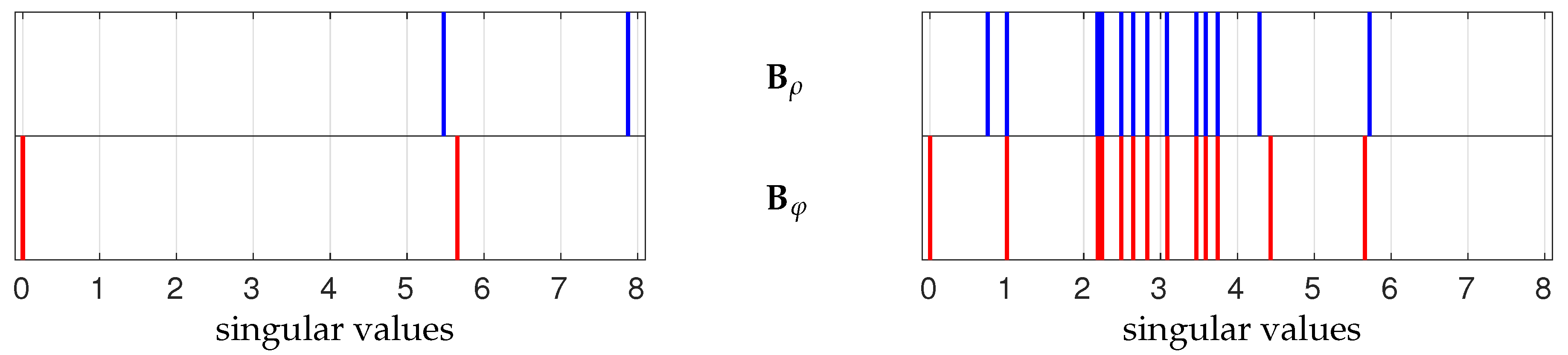
6.1. Sensitivity to Inversion Method

Shown in Figure 6 are simulated complex gains $\mathcal{G}$ for the 32 elementary antennas of the square array shown in Figure 3: the amplitudes and the phases were randomly chosen in the ranges $[-50\%,+50\%]$ and $[-\pi /3,+\pi /3]$, respectively. They were used for blurring the expected complex visibilities $V_{\odot }$ and simulating the measured ones $V_{\odot }^e$ according to (16), without adding any radiometric noise in the first attempt. The latter was processed for minimizing the cost functions (17) and (19) by solving (18) and (20) with the objective to retrieve the amplitude ${\alpha }_{\rho }$ and the phase ${\alpha }_{\phi }$ of every $\mathcal{G}$. The retrieved gains obtained $\tilde{\mathcal{G}}$ thus far are shown in Figure 6 for comparison with $\mathcal{G}$. Although the inversions were reduced to ${\mathbf{B}}^{+}$ for both the amplitude (13a) and the phase (13b), it turns out that in the absence of any radiometric noise and with small phase errors introduced at the elementary antenna level, i.e., $|{\alpha }_{\phi }| < \pi /2$, the reconstruction is perfect since $\tilde{\mathcal{G}}=\mathcal{G}$, according to the values of both $\mathrm{RMSE}\left({\tilde{\alpha }}_{\rho }\right)$ and $\mathrm{RMSE}\left({\tilde{\alpha }}_{\phi }\right)$.

Shown in Figure 7 are simulated complex gains $\mathcal{G}$ for the same 32 elementary antennas but with larger phase errors. The phases were again randomly chosen but in the range of $[-2\pi /3,+2\pi /3]$, whereas the amplitudes are those of the previous simulation in the range of $[-50\%,+50\%]$. Here, again, the inversions were reduced to ${\mathbf{B}}^{+}$ for both the amplitude (13a) and the phase (13b). In the absence of any radiometric noise, the reconstruction is still perfect on the amplitude side: As expected, $|\tilde{\mathcal{G}}|=|\mathcal{G}|$, according to the value of $\mathrm{RMSE}\left({\tilde{\alpha }}_{\rho }\right)$. On the contrary, this is not the case at the phase level, as expected again. Indeed, here, few components of ${\alpha }_{\phi }$ are larger than $\pi /2$, and as predicted in the previous section, this situation should end with unwrapping issues as soon as the reconstruction is reduced to the linear approach (19). This is exactly what is observed with few components, 22 out of 32, perfectly retrieved, while for the 10 others, the phase calibration residual error might be as large as 56°. More precisely, $\mathrm{RMSE}\left({\tilde{\alpha }}_{\phi }\right)$ is about 30° for these 10 antennas, whereas it is equal to 0° for the 22 others and about 17° when they are all taken into account.

It is interesting to note that those antennas ${\mathcal{A}}_p$ with a large residual phase error ${\tilde{\alpha }}_{\phi ;p}-{\alpha }_{\phi ;p}$ are those with an initial phase error $|{\alpha }_{\phi ;p}| > \pi /2$, but also, a few other antennas show $|{\alpha }_{\phi :p}| < \pi /2$. This is not surprising, as solving a linear system is an overall process where each component of the solution is a linear combination of the constant terms. On the contrary, it is surprising that few components are not affected by the phase unwrapping issue. Although no rational explanation has been found, it might be a proof of the robustness of the problem.

The true complex visibilities $V_{\odot }^{\phantom{e}}$ of the beacon located in ${\mathit{\xi }}_{\odot }=(0.3,0.2)$ are shown in Figure 8. To extend the study beyond the retrieved antenna gains, they are compared to the experimental gains $V_{\odot }^e$ and to the calibrated gains $V_{\odot }^c$ obtained with the simulated gains $\mathcal{G}$ and with the estimated gains $\tilde{\mathcal{G}}$, respectively, shown in Figure 7. Here, $\mathrm{RMSE}\left(V_{\odot }^e\right)$ is about $1.08$ K as a result of the effect of the complex gains $\mathcal{G}$ introduced in the simulation. As a consequence of the phase calibration residual errors still present at the end of the calibration process with $\mathrm{RMSE}\left({\tilde{\alpha }}_{\phi }\right)$ ≃ 17°, the calibrated visibilities do not match those of the beacon, as illustrated here by $\mathrm{RMSE}\left(V_{\odot }^c\right)\simeq 0.36$ K, although $\mathrm{RMSE}\left({\tilde{\alpha }}_{\rho }\right)=0$: clearly, calibration is a process where both amplitude and phase of the antenna gains have to be retrieved accurately. To have an idea of the importance of this error at the visibility level, it has to be compared to the random radiometric noise that may affect them and which, all else being equal, would be of the order of $0.12$ K here for a typical integration time of 1 s in the 1400–1427 MHz protected band [59]. As a consequence, the poor accuracy obtained here with this approach is clearly unsatisfactory, as it was feared in Section 5 when addressing phase calibration problems with the linear approach (19). This method therefore has to be definitively abandoned unless there is a guarantee to be in a situation with small antenna phases...but no one will take the risk to make this bet.

The Fourier transform [60] of an image results in both an amplitude spectrum and a phase spectrum. It is well known that most of the information contained in an image is transported by the phase spectrum and not by the amplitude spectrum, as very well illustrated in Figure 1 in [61]. It would therefore not be a surprise to see that this is also the case with complex visibilities. This is exactly what is revealed in Figure 9 with the Point-Spread Functions (PSFs) obtained from the inversion of the complex visibilities in Figure 8 according to (5). Here, again, it is clear that linear approach (19) is not an appropriate solution to the phase calibration problem as the artifacts in the PSF obtained thus far are too important for aperture synthesis imaging applications.

As argued in Section 5 and illustrated in Figure 7 and Figure 9, the phase of the complex visibilities $V_{\odot }^e$ should not be roughly unwrapped when minimizing the linear least-squares functional (19). On the contrary, it has to be carried out progressively while minimizing the non-linear least-squares functional (21) with the aid of iterative Algorithm 1 where linearized Equation (22) is solved at each iteration of the optimization process. Shown in Figure 10 are the retrieved complex gains $\tilde{\mathcal{G}}$ obtained under the same conditions as those of Figure 7 but after only 4 iterations of Algorithm 1 for retrieving 32 unknown phases. As expected, in the absence of any radiometric noise, the reconstruction is perfect since $\tilde{\mathcal{G}}=\mathcal{G}$, according to the values of both $\mathrm{RMSE}\left({\tilde{\alpha }}_{\rho }\right)$ and $\mathrm{RMSE}\left({\tilde{\alpha }}_{\phi }\right)$, and contrary to what was obtained when the phase of $V_{\odot }^e$ was unwrapped without any precaution. It is not necessary to check the calibrated visibilities $V_{\odot }^c$ here as it is now evident that $\mathrm{RMSE}\left(V_{\odot }^c\right)=0$ K.

For an idea of how iterative Algorithm 1 behaves, the retrieved complex gains $\tilde{\mathcal{G}}$ obtained at each iteration are shown in Figure 11. When starting from a null phase for every elementary antenna, the phases are retrieved in ascending order, from the very smallest ones to the largest. Consequently, exploring values beyond the interval $[-\pi /2,\pi /2]$ does not raise any difficulty, as illustrated by the transition from the second to the third iteration.

Finally, as soon as the temperature $T_{\odot }$ and the location ${\mathit{\xi }}_{\odot }$ of the beacon are known, the calibration does not create any problem. All the simulations conducted with a beacon located at another place in the field of view and with an other brightness temperature led to the same performances. The next sections move away from this ideal setting by introducing biases, errors, and noises that may perturb the calibration.

6.2. Sensitivity to Amplitude and Phase Biases

In the previous simulations, the amplitudes ${\alpha }_{\rho }$ and the phases ${\alpha }_{\phi }$ of the 32 complex gains $\mathcal{G}$ were randomly chosen in the ranges $[-50\%,+50\%]$ and $[-2\pi /3,+2\pi /3]$ with random distributions centered on zero: $\langle {\alpha }_{\rho }\rangle =0$, or equivalently, $\langle e^{{\alpha }_{\rho }}\rangle =1$ and $\langle {\alpha }_{\phi }\rangle$= 0°. Simulations conducted here were affected by a systematic error [62]. More specifically, a negative bias of $20\%$ was introduced in the amplitudes of $\mathcal{G}$, so that, now, $\langle e^{{\alpha }_{\rho }}\rangle =0.8$, and at the same time, a positive bias of 10° was introduced in the phases of $\mathcal{G}$, so that, now, $\langle {\alpha }_{\phi }\rangle$ = 10°. Here, again, amplitude calibration was reduced to ${\mathbf{B}}_{\rho }^{+}$ for solving (18), or equivalently, for minimizing (17) while phase calibration is performed with the aid of Algorithm 1 which makes intensive use of ${\mathbf{B}}_{\phi }^{+}$ for solving (22) at each iteration of the global minimization of (21).

Shown in Figure 12 are the retrieved complex gains $\tilde{\mathcal{G}}$. In the absence of any radiometric noise, the reconstruction is still perfect on the amplitude side: as expected, $|\tilde{\mathcal{G}}|=|\mathcal{G}|$, according to the value of $\mathrm{RMSE}\left({\tilde{\alpha }}_{\rho }\right)=0\%$. On the contrary, this is not the case at the phase level, as expected again, since, here, $\mathrm{RMSE}\left({\tilde{\alpha }}_{\phi }\right)$ = 10°. However, the distribution of this error over the 32 elementary antennas is that of a reconstruction bias and not that of a random error. Indeed, it turns out that every retrieved phase ${\tilde{\alpha }}_{\phi }$, regardless of its value, is exactly equal to ${\alpha }_{\phi }$ − 10°, as a consequence of the propagation of the 10° positive bias introduced in the phases of $\mathcal{G}$ through the phase calibration process.

As shown in Appendix A, the antenna function space F, here, of dimension $N_a=32$, is decomposed into $F_0$, the one-dimensional space of constant functions, and its orthogonal complement $F_1$, the space of dimension 31 of the functions of F with a mean value of zero. With regard to the linear operator ${\mathbf{B}}_{\phi }$ involved in phase calibration, it turns out that $F_0=ker{\mathbf{B}}_{\phi }$, which is the null space of ${\mathbf{B}}_{\phi }$. On the contrary, the linear operator ${\mathbf{B}}_{\rho }$ in terms of amplitude calibration is of full rank: $ker{\mathbf{B}}_{\rho }=\varnothing$. 3 As a consequence of the orthogonal decomposition $F=F_0\oplus F_1$, the minimum-norm solution ${\tilde{\alpha }}_{\phi }$ is obtained in $F_1$, the orthogonal of $ker{\mathbf{B}}_{\phi }$, with the corresponding signature $\langle {\tilde{\alpha }}_{\phi }\rangle$ = 0°, by definition of $F_1$. It is therefore not surprising to see the (constant) bias still present in that solution as it belongs to $F_0=ker{\mathbf{B}}_{\phi }$. This is not the case for ${\tilde{\alpha }}_{\rho }$ which belongs to $F=F_0\oplus F_1$ and is therefore not constrained to satisfy the relation $\langle {\tilde{\alpha }}_{\rho }\rangle =0$, by definition of $F_0$ and $F_1$.

Finally, shown in Figure 13 are the complex visibilities $V_{\odot }^{\phantom{e}}$ of the beacon located in ${\mathit{\xi }}_{\odot }=(0.3,0.2)$. They are compared to the experimental visibilities $V_{\odot }^e$ and to the calibrated visibilities $V_{\odot }^c$ obtained with the simulated gains $\mathcal{G}$ and with the estimated gains $\tilde{\mathcal{G}}$, respectively, as shown in Figure 12. $\mathrm{RMSE}\left(V_{\odot }^e\right)$ is about $0.92$ K as a result of the effect of the complex gains $\mathcal{G}$ introduced in the simulation. Although there is a phase calibration residual bias still present at the end of the calibration process with $\mathrm{RMSE}\left({\tilde{\alpha }}_{\phi }\right)={10}^{\circ }$, thanks to $\mathrm{RMSE}\left({\tilde{\alpha }}_{\rho }\right)=0$, the calibrated visibilities perfectly match those of the beacon, as illustrated here by $\mathrm{RMSE}\left(V_{\odot }^c\right)=0$ K. This is expected when referring back to (10b), as any antenna phase bias ${\overline{\alpha }}_{\phi }$ has strictly no impact on the experimental baseline phase ${\beta }_{\phi }^e$ because it cancels out according to $({\alpha }_{\phi ;p}+{\overline{\alpha }}_{\phi })-({\alpha }_{\phi ;q}+{\overline{\alpha }}_{\phi })+{\beta }_{\phi ;pq}={\alpha }_{\phi ;p}-{\alpha }_{\phi ;q}+{\beta }_{\phi ;pq}={\beta }_{\phi ;pq}^e$. If the presence of the one-dimensional kernel of constant phases $ker{\mathbf{B}}_{\phi }$ had the side effect just discussed earlier in this section at the level of the retrieval of the antenna complex gains $\tilde{\mathcal{G}}$, as illustrated in Figure 12, it would also have this nice effect thanks to the annihilation property ${\mathbf{B}}_{\phi }\mathbf{A}=0$ established in Appendix A, so that, finally, it can be stated that the antenna phase bias is definitely not an issue in phase calibration, as was very intuitively expected.

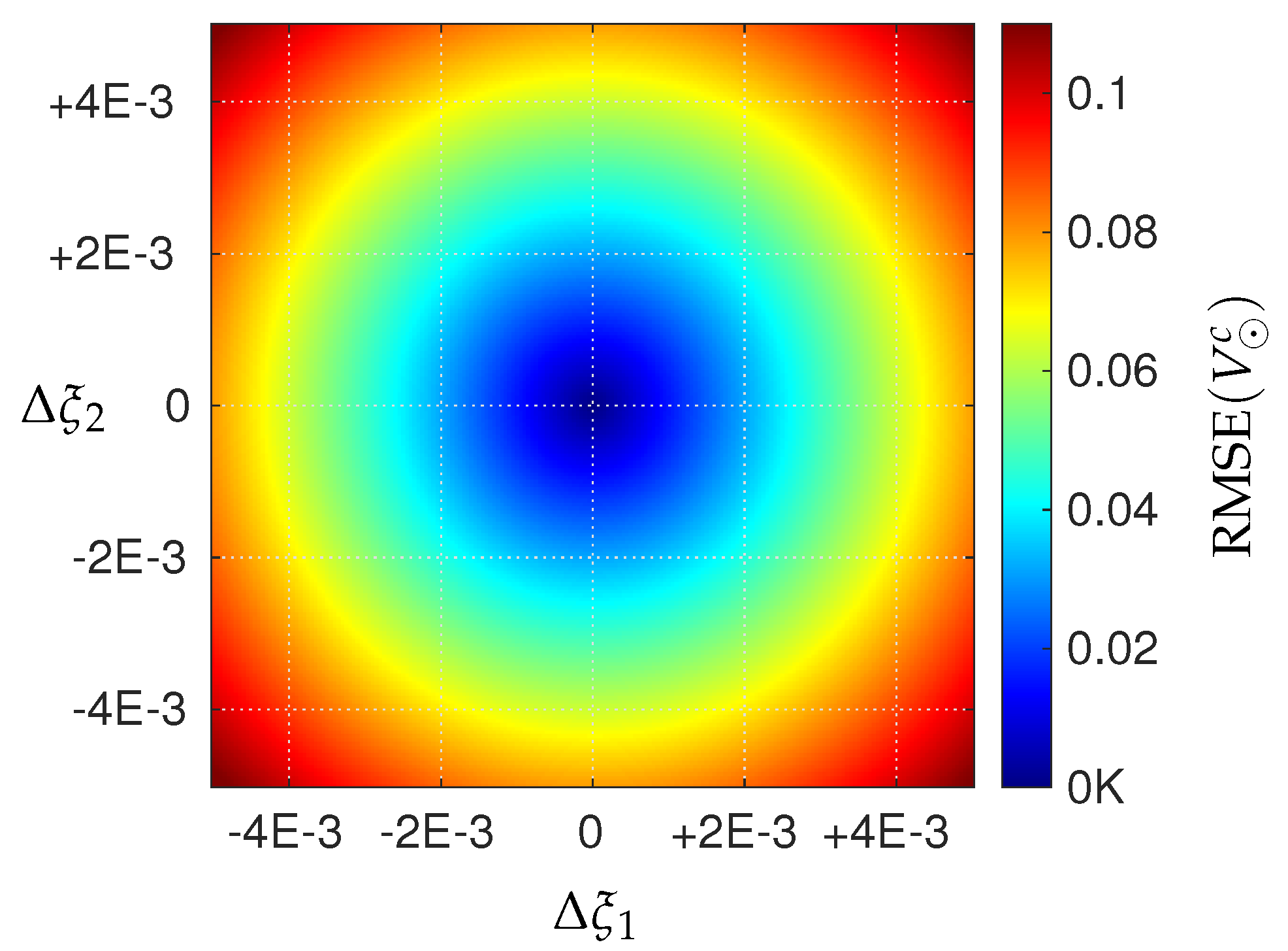
6.3. Sensitivity to Mislocation of Beacon

Simulations were performed with amplitudes ${\alpha }_{\rho }$ and phases ${\alpha }_{\phi }$ of the 32 complex gains $\mathcal{G}$ randomly chosen in the ranges of $[-50\%,+50\%]$ and $[-2\pi /3,+2\pi /3]$ (those in red in Figure 7 and Figure 10) and for the same sets of complex visibilities $V_1^e$ and $V_2^e$, but, here, an unknown error $\Delta \mathit{\xi }$ was introduced in the location of the beacon in ${\mathit{\xi }}_{\odot }=(0.3,0.2)$. The two components $\Delta {\xi }_1$ and $\Delta {\xi }_2$ of the position error $\Delta \mathit{\xi }$ were chosen in the range of $[-0.005,+0.005]$, that is to say, approximately [−0.3°, +0.3°]. Referring back to Figure 9, it turns out that it is about an eleventh of the angular resolution. Amplitude calibration was still reduced to ${\mathbf{B}}_{\rho }^{+}$ for solving (18), or equivalently, for minimizing (17), while phase calibration was performed again with the aid of Algorithm 1 which makes intensive use of ${\mathbf{B}}_{\phi }^{+}$ for solving (22) at each iteration of the global minimization of (21).

Shown in Figure 14 is an example of retrieved complex gains $\tilde{\mathcal{G}}$ when an unknown uncertainty of 0.3° is introduced on both coordinates $\Delta {\xi }_1$ and $\Delta {\xi }_2$. Although there is still no radiometric noise introduced in the complex visibilities, the calibration is no longer perfect as illustrated by $\mathrm{RMSE}\left({\tilde{\alpha }}_{\rho }\right)\simeq 0.5\%$ and $\mathrm{RMSE}\left({\tilde{\alpha }}_{\phi }\right)$ ≃ 5°. It can be observed that there is no evidence for some antennas ${\mathcal{A}}_p$ to be more, or less, affected by these errors than others.

The same experiment was conducted with further uncertainties. Shown in Figure 15 are the corresponding RMSEs at the level of the retrieved complex gains $\tilde{\mathcal{G}}$ for every position error introduced. Of course, when $\Delta \mathit{\xi }=(0,0)$, the inversions are those of Figure 10. On the contrary, as soon as an unknown uncertainty on the position of the beacon is introduced, it translates into errors in the retrieved components ${\tilde{\alpha }}_{\rho }$ and ${\tilde{\alpha }}_{\phi }$ of the estimated complex gains $\tilde{\mathcal{G}}$. The distribution of these two errors with respect to that of $\Delta \mathit{\xi }$ shows two behaviors: the RMSE of ${\tilde{\alpha }}_{\phi }$ is centro-symmetric, whereas that of ${\tilde{\alpha }}_{\rho }$ clearly depends on the azimuth of the beacon with respect to the phase center of the array. At this level, no conclusion can be drawn on the importance of one component with regard to the other. Shown in Figure 16 is the distribution of the corresponding RMSE at the level of the calibrated visibilities $V_{\odot }^c$. Here, again, in the absence of any radiometric noise introduced in the complex visibilities, when $\Delta \mathit{\xi }=(0,0)$, the calibration is perfect. On the contrary, any unknown uncertainty $\Delta \mathit{\xi }$ on the position ${\mathit{\xi }}_{\odot }$ of the beacon translates into an error in $V_{\odot }^c$ when compared to $V_{\odot }$. Referring back to the two distributions shown in Figure 15 and comparing both with that of Figure 16, it can be concluded that the phase estimation ${\tilde{\alpha }}_{\phi }$ is more sensitive to unknown uncertainties on the position of the beacon than amplitude estimation ${\tilde{\alpha }}_{\rho }$ because the variations in $\mathrm{RMSE}\left(V_{\odot }^c\right)$ with $\Delta \mathit{\xi }$ are clearly those of $\mathrm{RMSE}\left({\tilde{\alpha }}_{\phi }\right)$ and not those of $\mathrm{RMSE}\left({\tilde{\alpha }}_{\rho }\right)$. Here, again, this error at the visibility level has to be compared to the random radiometric noise that may affect them and which, all other things remaining equal, would be of the order of $0.12$ K here for a typical integration time of 1 s in the 1400–1427 MHz protected band [59]. As a consequence, uncertainties about the position of the beacon as large as an eleventh of the angular resolution, i.e., 0.3°, would be responsible for an RMSE at a visibility level of the same order as the standard deviation of the random radiometric noise when observing a scene at a constant temperature of 300 K during a typical integration time of 1 s in a 27 MHz band. To fix the ideas more concretely, for an experiment conducted with a ground-based instrument suspended on top of a crane from an elevation of $h=20$ m, an uncertainty of 0.3° translates into a requirement of 10 cm regarding the precision with which the position of the beacon must be known in the field of view.

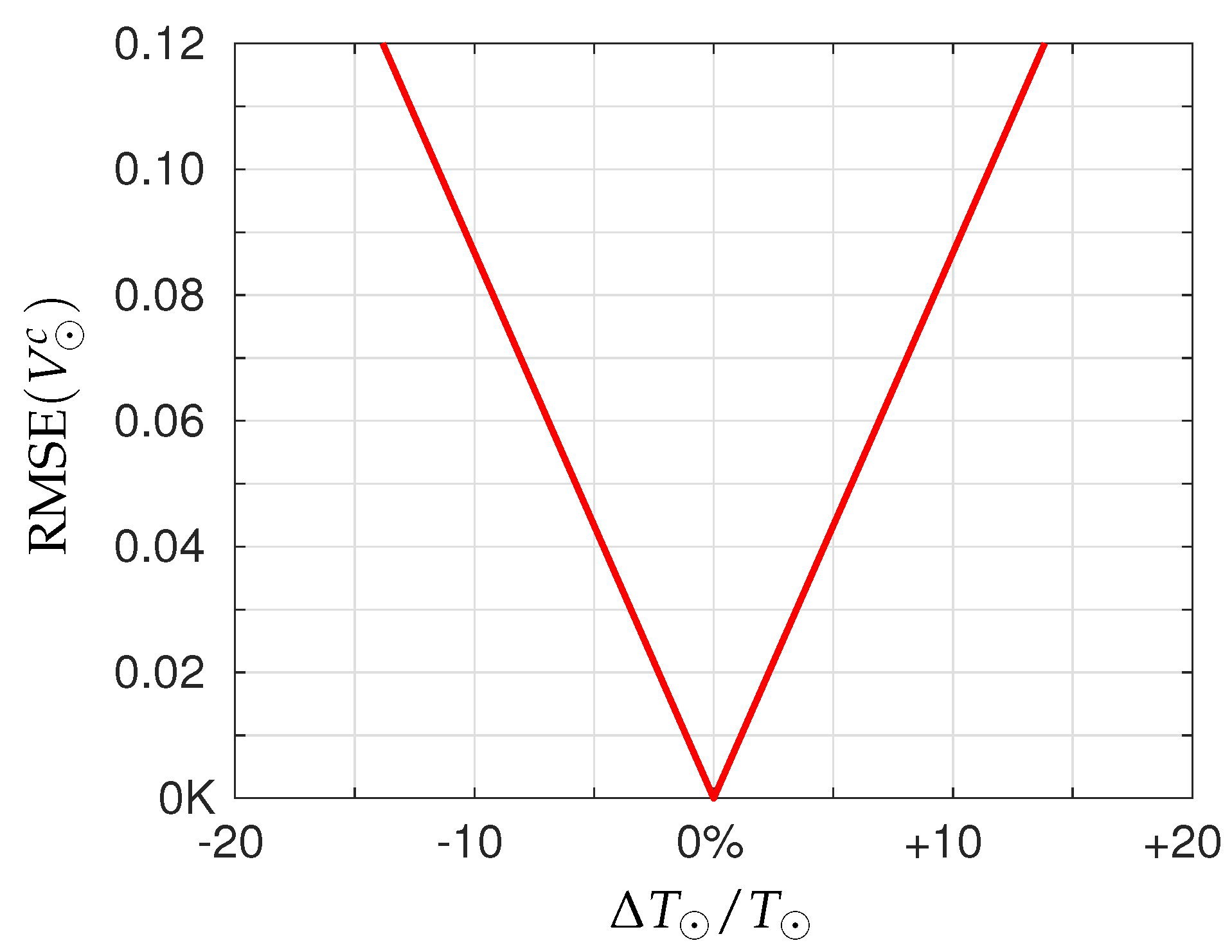
6.4. Sensitivity to Wrong Temperature of Beacon

Another parameter of the beacon whose imperfect knowledge must be taken into account is its brightness temperature. This is why simulations were performed with amplitudes ${\alpha }_{\rho }$ and phases ${\alpha }_{\phi }$ of the 32 complex gains $\mathcal{G}$ randomly chosen in the ranges of $[-50\%,+50\%]$ and $[-2\pi /3,+2\pi /3]$ (those in red in Figure 7 and Figure 10) and for the same sets of complex visibilities $V_1^e$ and $V_2^e$, but, here, an unknown error $\Delta T_{\odot }$ was introduced on the brightness temperature $T_{\odot }$ of the beacon in ${\mathit{\xi }}_{\odot }=(0.3,0.2)$. Amplitude calibration was still reduced to ${\mathbf{B}}_{\rho }^{+}$ for solving (18), or equivalently, for minimizing (17), while phase calibration was performed again with the aid of Algorithm 1.

Shown in Figure 17 is an example of retrieved complex gains $\tilde{\mathcal{G}}$ when the unknown uncertainty $\Delta T_{\odot }$ is equal to $15\%$ of the brightness temperature $T_{\odot }$ of the beacon. Although there is still no radiometric noise introduced in the complex visibilities, the amplitude calibration is no longer perfect as illustrated by $\mathrm{RMSE}\left({\tilde{\alpha }}_{\rho }\right)\simeq 8\%$. On the contrary, this kind of error does not affect the phase calibration as expected as illustrated by $\mathrm{RMSE}\left({\tilde{\alpha }}_{\phi }\right)$ ≃ 0°.

The same experiment was conducted with further uncertainties. Shown in Figure 18 are the variations of the corresponding RMSE at the level of the calibrated visibilities $V_{\odot }^c$. Here, again, in the absence of any radiometric noise introduced in the complex visibilities, when $\Delta T_{\odot }=0$ K, the calibration is perfect. On the contrary, any unknown uncertainty $\Delta T_{\odot }$ on the brightness temperature $T_{\odot }$ of the beacon translates into an error in $V_{\odot }^c$ when compared to $V_{\odot }$. Here, again, this error at the visibility level has to be compared to the random radiometric noise that may affect them and which, all other things remaining equal, would be of the order of $0.12$ K here for a typical integration time of 1 s in the 1400–1427 MHz protected band [59]. As a consequence, uncertainties on the brightness temperature of the beacon as large as ±15% would be responsible for an RMSE at a visibility level of the same order of the standard deviation of the random radiometric noise when observing a scene at a constant temperature of 300 K during a typical integration time of 1 s in a 27 MHz band.

6.5. Sensitivity to Missing Baselines

In aperture synthesis, the baselines ${\mathbf{b}}_{pq}$ between pairs of elementary antennas ${\mathcal{A}}_p$ and ${\mathcal{A}}_q$ of an array sample the so-called uv plane. The set of points obtained thus far is called the uv coverage of the antenna array. When different pairs of elementary antennas lead to the same point of the uv coverage, they are said to be redundant. This is the case for many baselines of the square array shown in Figure 3. When all the elementary antennas are present in the list of available complex visibilities $V_{\odot ;pq}^e$ used for minimizing (17) and (21), there should be no reason why it should not be possible to calibrate the antenna array. However, the accuracy of the retrieved antenna gains $\tilde{\mathcal{G}}$ may vary with the number of missing baselines. The location of these missing baselines may also be a driver of the calibration performances since the redundancy of the baselines clearly has an impact on the minimization. Finally, before going into the details of this analysis, it should be mentioned that when baselines are missing, the expressions (13a) and (13b) of the pseudo-inverses ${\mathbf{B}}_{\rho }^{+}$ and ${\mathbf{B}}_{\phi }^{+}$ are no longer valid. Since there is a very large number of possible situations, it is hopeless to expect a theoretical expression that would be valid for every case, regardless of the antenna array. This is why, here, ${\mathbf{B}}_{\rho }^{+}$ and ${\mathbf{B}}_{\phi }^{+}$ were estimated numerically with the aid of a computer (for Matlab users, by calling the function pinv).

Shown in Figure 19 is the uv coverage of the square array shown in Figure 3 for two very distinct situations with the same number of elementary antennas: $N_a=32$. On one hand, all the $N_b=N_a(N_a-1)/2=496$ pairs of antennas are used. Owing to the geometry of the array, some points of the uv coverage are redundant and the level of redundancy varies from 1 (non-redundant) to 18 (the most redundant). On the other hand, only a few of these pairs are used here, exactly 112, so that the level of redundancy is now equal to one for every point of the uv coverage. It is therefore natural to question the impact of the 384 missing baselines in the calibration of the complex gains of the 32 elementary antennas. Indeed, in the first situation, the size of the aberration matrices to be inverted is $496\times 32$, whereas in the second situation, it is only $112\times 32$. As a consequence of this reduction in the amount of data for the same number of unknowns to retrieve, some effect can be expected from the linear algebra point of view on the property of the corresponding matrices. This is what is illustrated in Figure 20 with the singular values of ${\mathbf{B}}_{\rho }$ and ${\mathbf{B}}_{\phi }$ where a partial breaking of degeneracies is observed for both aberration matrices: from only 2 unique singular values with multiplicity values of 1 and 31 ($\sqrt{N_a-2}\simeq 5.48$ and $\sqrt{2N_a-2}\simeq 7.87$ for ${\mathbf{B}}_{\rho }$ and 0 and $\sqrt{N_a}\simeq 5.66$ for ${\mathbf{B}}_{\phi }$, as demonstrated in Appendix A) to 13 different values with their multiplicity values varying between 1 and 11. With regard to the phase aberration operator ${\mathbf{B}}_{\phi }$, attention should be focused on the null singular value with a multiplicity of 1 which is still associated with a kernel of dimension 1. Concerning the amplitude aberration operator ${\mathbf{B}}_{\rho }$, the kernel is still reduced to the empty set as the smallest singular value is different from 0. As a consequence of this new distribution of the singular values, which preserves the main properties of both aberration matrices, a behavior very similar to what has been observed so far is expected.

Shown in Figure 21 are the retrieved complex gains $\tilde{\mathcal{G}}$ with only 112 pairs of elementary antennas. They have to be compared to those retrieved with all the 496 pairs shown in Figure 10. It turns out that the reconstruction is perfect on the amplitude side, according to the value of $\mathrm{RMSE}\left({\tilde{\alpha }}_{\rho }\right)=0\%$. This is not the case at the phase level since, here, $\mathrm{RMSE}\left({\tilde{\alpha }}_{\phi }\right)$ = 12°. However, the distribution of this error over the 32 elementary antennas is that of a reconstruction bias and not that of a random error. Indeed, it turns out that, here, every retrieved phase ${\tilde{\alpha }}_{\phi }$ is exactly equal to ${\alpha }_{\phi }$ − 12°. As a consequence, the situation is similar to that encountered in Figure 12 where a phase bias was introduced in the phases ${\alpha }_{\phi }$ of $\mathcal{G}$ and the same bias was observed in the retrieved phases ${\tilde{\alpha }}_{\phi }$ of $\tilde{\mathcal{G}}$. According to Chapter 5 in [63], the idea of “same cause, same effect” persists, so that, thanks again to the annihilation property ${\mathbf{B}}_{\phi }\mathbf{A}=0$ established in Appendix A, the calibrated visibilities perfectly match those of the beacon as illustrated by $\mathrm{RMSE}\left(V_{\odot }^c\right)=0$ K in Figure 22. As a consequence, provided that all the elementary antennas are present in the antenna pairs corresponding to the available complex visibilities $V_{\odot }^e$, missing baselines are not an issue in phase calibration.

6.6. Sensitivity to Random Radiometric Noise

Finally, last but not least, referring back to (16), the complex visibilities $V_1^e$ and $V_2^e$ were blurred with different radiometric noises ${\eta }_1$ and ${\eta }_2$, which are distinct random draws of a centered Gaussian distribution with standard deviation ${\sigma }_{\eta }$. As a consequence of the composition of independent stochastic processes, the complex visibilities $V_{\odot }^e$ were still affected by a random Gaussian noise but with the standard deviation $\sqrt{2}{\sigma }_{\eta }$. Here, again, amplitude calibration was reduced to ${\mathbf{B}}_{\rho }^{+}$ for solving (18), or equivalently, for minimizing (17), while phase calibration was performed with the aid of Algorithm 1 which makes intensive use of ${\mathbf{B}}_{\phi }^{+}$ for solving (22) at each iteration of the global minimization of (21).

After 1000 random trials of radiometric noises ${\eta }_1$ and ${\eta }_2$ with the same standard deviation ${\sigma }_{\eta }\simeq 0.04$ K corresponding, here, to an integration time of 10 s in a 27 MHz bandwidth [59] and the estimation of $\tilde{\mathcal{G}}$ from the noisy $V_{\odot }^e$ for each of them, it turns out that $\mathrm{RMSE}\left({\tilde{\alpha }}_{\rho }\right)\simeq 0.9\%\pm 0.1\%$ and $\mathrm{RMSE}\left({\tilde{\alpha }}_{\phi }\right)$ ≃ 0.5° ± 0.08° when comparing them to $\mathcal{G}$. With regard to the complex visibilities, when comparing them to $V_{\odot }$, it turns out that $\mathrm{RMSE}\left(V_{\odot }^e\right)\simeq 1.09\mathrm{K}\pm 0.002\mathrm{K}$ and $\mathrm{RMSE}\left(V_{\odot }^c\right)\simeq 0.06\mathrm{K}\pm 0.002\mathrm{K}$. The latter has to be compared to the radiometric noise level $\sqrt{2}{\sigma }_{\eta }\simeq 0.05$ K. Shown in Figure 23 and Figure 24 are representative examples of such retrieved complex gains and visibilities.

The same experiment was conducted with a higher level of random radiometric noise. After 1000 random trials of ${\eta }_1$ and ${\eta }_2$ with the same standard deviation ${\sigma }_{\eta }\simeq 0.12$ K corresponding, now, to an integration time of 1 s in a 27 MHz bandwidth [59] and the estimation of $\tilde{\mathcal{G}}$ from the noisy $V_{\odot }^e$ for each of them, it turns out that $\mathrm{RMSE}\left({\tilde{\alpha }}_{\rho }\right)\simeq 2.8\%\pm 0.3\%$ and $\mathrm{RMSE}\left({\tilde{\alpha }}_{\phi }\right)$≃ 1.6° ± 0.3° when comparing them to $\mathcal{G}$. With regards to the complex visibilities, when comparing them to $V_{\odot }$, it turns out that $\mathrm{RMSE}\left(V_{\odot }^e\right)\simeq 1.10\mathrm{K}\pm 0.005\mathrm{K}$ and $\mathrm{RMSE}\left(V_{\odot }^c\right)\simeq 0.19\mathrm{K}\pm 0.006\mathrm{K}$. The latter has to be compared to the radiometric noise level $\sqrt{2}{\sigma }_{\eta }\simeq 0.16$ K. Shown in Figure 25 and Figure 26 are representative examples of such retrieved complex gains and visibilities.

It is obvious that the level of performance does not depend only on the amount of random radiometric noise but also on the power emitted by the beacon. More specifically, from the synthesis imaging point of view, it depends, here, on the signal-to-noise ratio (SNR) between the brightness temperature $T_{\odot }$ of the point source located in ${\mathit{\xi }}_{\odot }$ and the standard deviation $\sqrt{2}{\sigma }_{\eta }$ of the radiometric noise affecting the complex visibilities $V_{\odot }^e$. In the first case shown in Figure 23 and Figure 24, this SNR is about $42.9$ dB, whereas in the second case illustrated in Figure 25 and Figure 26, it is about $37.9$ dB as a consequence of an integration time $\sqrt{10}$ times smaller. In both cases, comparing the brightness temperature of the beacon $T_{\odot }$, set to 1000 K here, and the constant temperature of the background scene, set to 300 K here, is not relevant because the contribution of the latter to $V_{\odot }^e$ was removed, according to (16), so that the situation is clearly that which is illustrated in Figure 2 (right). This background distribution only has an effect through the additive random radiometric noises ${\eta }_1$ and ${\eta }_2$, according to (14) and (15). As a consequence, for the experiment simulated here, the uncertainty on the retrieved antenna gains is only driven by the ratio between the brightness temperature of the beacon and the level of the radiometric noise: the higher this ratio, the more accurate the retrieved complex gains.

7. Discussion

All the results presented in the previous section are based on numerical simulations conducted for the FANTASIOR project, a common R&D program of CNES and CESBIO which aims to record the radio signals maintained by elementary antennas operating in the 1400–1429 MHz frequency band for deferred processing with the aid of a computer. The idea is to perform digital beam forming or synthetic aperture interferometry in the protected band 1400–1427 MHz while using the service band 1427–1429 MHz for calibration purposes. It is clear that the brightness temperature $T_{\odot }$ seen by the antenna array with a beacon centered on 1428 MHz in the service band might not be that of a beacon emitting the same power but one centered on $f_o=1413.5$ MHz in the protected band, simply because the response of the elementary antennas may vary with frequency. However, it does not change the previous conclusions, including the very last ones about the role played by the signal-to-noise ratio. Finally, it is foreseen in the calibration plan of FANTASIOR to estimate the complex gains at a laboratory level (in an anechoic chamber) for different frequencies in order to check how manufacturing of the elementary antennas complies with specifications for calibrating the effective transfer function in the 1400–1427 MHz protected band from measurements acquired in the service band 1427–1429 MHz. As soon as FANTASIOR is available, the characterization of every elementary antenna and the calibration of the entire antenna array will be the subject of a forthcoming article.

It would have been great to assess these results with operational data from MIRAS on-board SMOS. It was explained in Section 4 why this was not possible and why it will definitely not be possible in the future. The main reason is due to the choices made during the design of MIRAS. As soon as the L-band is concerned, the frequency band 1400–1427 MHz is protected from any emission, as described in Section 1. The closest band that can be used for Earth-to-space emission is the service band 1427–1429 MHz, but MIRAS operates in the 19 MHz bandwidth from 1404 to 1423 MHz. This working frequency band cannot be shifted nor enlarged; as a consequence, the emission from a beacon centered on 1428 MHz in the service band is not visible to MIRAS, thus reducing the possibility to zero of estimating the effective transfer function with this approach to calibration.

When analyzing the results of Section 6, attention was first focused on the sensitivity of the retrieved complex gains to the inversion method. Amplitude calibration is not concerned with this line of questioning, but phase one is, owing to the particular role played by the phase, or the phasor, compared to that of the amplitude in a complex number. Previous studies considered that phase calibration can be performed accurately with a linear approach which roughly unwraps the phase, without taking precautions. The limits of this kind of approach have been described from a theoretical point of view in Section 5.2 and illustrated in Section 6.1 with results obtained in the ideal situation of very small antenna phases as well as in the situation of large phases. The observation is irrefutable: as soon as a few phases are outside $[-\pi /2,\pi /2]$, it is not possible to rely on such a linear approach. On the contrary, regardless of the distribution of the phases in $[-\pi ,\pi ]$, the non-linear approach introduced in Section 5.2 with Algorithm 1 is always reliable. Moreover, it is faster and simpler than other algorithmic approaches used in phase-closure imaging that tackle phase unwrapping by solving the integer ambiguity problem to account for the modulo $2\pi$ phases, but this is an unnecessary difficulty for phase calibration. As a consequence, in the absence of any errors, biases, or noises, the proposed algorithm does not suffer from any limitations.

Consideration was also given a second time to the sensitivity of the accuracy of the retrieved complex gains to various errors that may affect the complex visibilities. It was shown in Section 6.2 that both amplitude and phase calibration algorithms proposed here are not sensitive to amplitude biases nor to phase biases. At the same time, it has been verified in Section 6.6 that the sensitivity to radiometric noise is at the expected level. The effect of missing redundant baselines has been addressed in Section 6.5 and it turns out that it has no significant impact, provided that all the elementary antennas are involved in the calibration. Finally, the influence of an imperfect knowledge of the beacon has been studied in Section 6.3 with the introduction of a location error and in Section 6.4 with a brightness temperature error. The accuracy of the calibration was quantified in both cases, and it turns out that it can be maintained at an acceptable level. In conclusion, the proposed algorithm is of course sensitive to errors, biases, and noises, but their propagation is under control.

8. Conclusions

This article was devoted to the calibration of synthetic aperture interferometric radiometers. The effective transfer function of the antenna array has to be very well known for measuring accurate complex visibilities, and it is the role of the calibration to estimate the instrumental and environmental variations that may affect these interferometric measurements. This contribution has focused on the instrumental aspect of the calibration of the complex gains of every elementary antenna with the aid of a radio beacon. This approach is very similar to that used by radio-astronomers for calibrating the effective transfer function of radio-telescope arrays from complex visibilities obtained while observing quasi-stellar radio sources. If the amplitude calibration of complex gains does not raise any issue, then it was shown that phase calibration may bring up a serious challenge because the phase of complex visibilities cannot be roughly unwrapped. The risk of a wrong estimation of the complex gains was proven and illustrated. This problem was solved with the aid of a non-linear optimization algorithm for iteratively and smoothly unwrapping these phases. The performances of both amplitude and phase calibrations were assessed by means of numerical simulations conducted for the FANTASIOR project, a common R&D program of CNES and CESBIO which aims to record the radio signals maintained by elementary antennas for deferred processing with the aid of a computer.

All the results presented and discussed in this study were obtained with numerical simulations. However, they are based on strong theoretical foundations of an algebraic framework whose main elements of linear algebra are the key spaces and the key operators involved in the calibration of complex gains of elementary antennas. The amplitude and the phase aberration operators were introduced and their properties were fully demonstrated, in particular, their singular values and the theoretical expression of their pseudo-inverse. Although most of these elements can be found in the literature, for the sake of clarity and in the interest of pedagogy, notably, to make the reading of this article easier, an annex is included in order to bring together, in a single and unique place, the whole formalism of linear algebra introduced in several references. At the same time, this annex provides demonstrations not available in the literature because, for historical reasons, the phase was the main focus of studies while the amplitude was somewhat neglected. This is not the case in this article where both amplitude and phase calibrations were given the same attention, theoretically as well as numerically.

References

1. Ulaby, F.; Moore, R.; Fung, A. Microwave Remote Sensing—Active and Passive, 1st ed.; Artech House: Norwood, MA, USA, 1981. [Google Scholar]
2. Bracewell, R.N.; Roberts, J.A. Aerial Smoothing in Radio Astronomy. Aust. J. Phys. 1954, 7, 615–640. [Google Scholar]
3. Ryle, M.; Hewish, A. The Synthesis of Large Radio Telescopes. Mon. Not. R. Astron. Soc. 1960, 120, 220–230. [Google Scholar] [CrossRef]
4. Ruf, C.S.; Swift, C.T.; Tanner, A.B.; Le Vine, D.M. Interferometric synthetic aperture microwave radiometry for the remote sensing of the Earth. IEEE Trans. Geosci. Remote Sens. 1988, 26, 597–611. [Google Scholar] [CrossRef]
5. Corbella, I.; Duffo, N.; Vall-llossera, M.; Camps, A.; Torres, A. The Visibility Function in Interferometric Aperture Synthesis Radiometry. IEEE Trans. Geosci. Remote Sens. 2004, 42, 1677–1682. [Google Scholar] [CrossRef]
6. Anterrieu, É. A Resolving Matrix Approach for Synthetic Aperture Imaging Radiometers. IEEE Trans. Geosci. Remote Sens. 2004, 42, 1649–1656. [Google Scholar] [CrossRef]
7. Thompson, A.R.; Moran, J.W.; Swenson, G.W. Interferometry and Synthesis in Radio Astronomy, 3rd ed.; Springer International Publishing: Cham, Switzerland, 2017. [Google Scholar]
8. Barré, H.; Duesmann, B.; Kerr, Y.H. SMOS: The Mission and the System. IEEE Trans. Geosci. Remote Sens. 2008, 46, 587–593. [Google Scholar] [CrossRef]
9. Amiot, T.; Goldstein, C. Impact of calibration on the performance of a total power radiometer. In Proceedings of the IEEE International Geoscience And Remote Sensing Symposium (IGARSS 2007), Barcelona, Spain, 23–28 July 2007. [Google Scholar]
10. McMullan, K.D.; Brown, M.A.; Martín-Neira, M.; Rits, W.; Ekholm, S.; Lemanczyk, J. SMOS: The Payload. IEEE Trans. Geosci. Remote Sens. 2008, 46, 594–605. [Google Scholar] [CrossRef]
11. Torres, F.; Camps, A.; Bara, J.; Corbella, I.; Ferrero, R. On-board phase and modulus calibration of large aperture synthesis radiometers: Study applied to MIRAS. IEEE Trans. Geosci. Remote Sens. 1996, 34, 1000–1009. [Google Scholar] [CrossRef]
12. El Maghraby, A.K.S.; Grubisic, A.; Colombo, C.; Tatnall, A. A novel interferometric microwave radiometer concept using satellite formation flight for geostationary atmospheric sounding. IEEE Trans. Geosci. Remote Sens. 2018, 56, 3487–3498. [Google Scholar] [CrossRef]
13. Connolly, R. Types of NDB. Radio User 2016, 11, 48–49. [Google Scholar]
14. El Maghraby, A.K.S.; Park, H.; Camps, A.; Grubisic, A.; Colombo, C.; Tatnall, A. Phase and Baseline Calibration for Microwave Interferometric Radiometers Using Beacons. IEEE Trans. Geosci. Remote Sens. 2020, 58, 5242–5253. [Google Scholar] [CrossRef]
15. Taylor, G.B.; Carilli, C.L.; Perley, R.A. (Eds.) Synthesis Imaging in Radio Astronomy II. In ASP Conference Series; The University of New Mexico: Albuquerque, NM, USA, 1999; Volume 180. [Google Scholar]
16. Sostronek, M.; Matejcek, M.; Baráni, Z. Design and Implementation of Output Circuitry for Millimeter-wave Direct Detection Radiometer. Sci. Mil. 2023, 18, 16–20. [Google Scholar] [CrossRef]
17. IEEE 521-2019; IEEE Standard Letter Designations for Radar-Frequency Bands. IEEE Standards Association: Piscataway, NJ, USA, 2020.
18. European Communications Office. The Protection of the Earth Exploration-Satellite Service (passive) in the 1400–1427 MHz Band. In Proceedings of the Minutes of the 44th Meeting of the Electronic Communications Committee, Dublin, Ireland, 28 February–3 March 2017. Available online: https://docdb.cept.org/ (accessed on 16 March 2025).
19. Anterrieu, É.; Cabot, F.; Kerr, Y.H.; Amiot, T.; Valat, D.; Lestarquit, L. Synchronization of Radio Signals for the Unconnected L-Band Interferometer Demonstrator (ULID). In Proceedings of the IEEE International Geoscience And Remote Sensing Symposium (IGARSS 2021), Brussels, Belgium, 12–16 July 2021. [Google Scholar]
20. Hagen, J.B.; Farley, D.T. Digital-Correlation Techniques in Radio Science. Radio Sci. 1973, 8, 775–784. [Google Scholar] [CrossRef]
21. Ko, H. Coherence theory of radio-astronomical measurements. IEEE Trans. Antennas Propag. 1967, 15, 10–20. [Google Scholar] [CrossRef]
22. Swenson, G.W.; Mathur, N.C. The interferometer in radio astronomy. Proc. IEEE 1968, 56, 2114–2130. [Google Scholar] [CrossRef]
23. Allen, J.L. Array antennas: New applications for an old technique. IEEE Spectr. 1964, 1, 115–130. [Google Scholar] [CrossRef]
24. Wijnholds, S.J.; van der Tol, S.; Nijboer, R.; van der Veen, A.-J. Calibration challenges for future radio telescopes. IEEE Signal Process. Mag. 2010, 27, 30–42. [Google Scholar] [CrossRef]
25. Grobler, T.L.; Nunhokee, C.D.; Smirnov, O.M.; van Zyl, A.J.; de Bruyn, A.G. Calibration artefacts in radio interferometry–I. Ghost sources in Westerbork Synthesis Radio Telescope data. Mon. Not. R. Astron. Soc. 2014, 439, 4030–4047. [Google Scholar] [CrossRef]
26. Wijnholds, S.J.; Grobler, T.L.; Smirnov, O.M. Calibration artefacts in radio interferometry–II. Ghost patterns for irregular arrays. Mon. Not. R. Astron. Soc. 2016, 457, 2331–2354. [Google Scholar] [CrossRef]
27. Grobler, T.L.; Stewart, A.J.; Wijnholds, S.J.; Kenyon, J.S.; Smirnov, O.M. Calibration artefacts in radio interferometry–III. Phase-only calibration and primary beam correction. Mon. Not. R. Astron. Soc. 2016, 461, 2975–2992. [Google Scholar] [CrossRef]
28. Anterrieu, É.; Lafuma, P.; Jeannin, N. An Algebraic Comparison of Synthetic Aperture Interferometry and Digital Beam Forming in Imaging Radiometry. Remote Sens. 2022, 14, 2285. [Google Scholar] [CrossRef]
29. van Cittert, P.H. Die Wahrscheinliche Schwingungsverteilung in Einer von Einer Lichtquelle Direkt Oder Mittels Einer Linse Beleuchteten Ebene. Physica 1934, 1, 201–210. [Google Scholar] [CrossRef]
30. Zernike, F. The Concept of Degree of Coherence and its Application to Optical Problems. Physica 1934, 5, 785–795. [Google Scholar] [CrossRef]
31. Anterrieu, É.; Yu, L.; Jeannin, N. A Comprehensive Comparison of Far-Field and Near-Field Imaging Radiometry in Synthetic Aperture Interferometry. Remote Sens. 2024, 16, 3584. [Google Scholar] [CrossRef]
32. Selvan, K.T.; Janaswamy, R. Fraunhofer and Fresnel Distances: Unified Derivation for Aperture Antennas. IEEE Antennas Propag. Mag. 2017, 59, 12–15. [Google Scholar] [CrossRef]
33. Hansen, P.C. Rank-Deficient and Discrete Ill-Posed Problems, 1st ed.; Society for Industrial & Applied Mathematics: Philadelphia, PA, USA, 1998. [Google Scholar]
34. Picard, B.; Anterrieu, E. Comparizon of regularized inversion methods in synthetic aperture imaging radiometry. IEEE Trans. Geosci. Remote Sens. 2005, 43, 218–224. [Google Scholar] [CrossRef]
35. Goodberlet, M.A. Improved Image Reconstruction Techniques for Synthetic Aperture Radiometers. IEEE Trans. Geosci. Remote Sens. 2000, 38, 1362–1366. [Google Scholar] [CrossRef]
36. Penrose, R. A generalized inverse for matrices. Math. Proc. Camb. Philos. Soc. 1955, 51, 406–413. [Google Scholar] [CrossRef]
37. Hansen, P.C. The Truncated SVD as a Method for Regularization. BIT Numer. Math. 1987, 27, 534–553. [Google Scholar] [CrossRef]
38. Smithies, F. The Eigen-Values and Singular Values of Integral Equations. Proc. Lond. Math. Soc. 1938, 43, 255–279. [Google Scholar] [CrossRef]
39. Cornwell, T.J.; Wilkinson, P.N. A new method for making maps with unstable radio interferometers. Mon. Not. R. Astron. Soc. 1981, 196, 1067–1086. [Google Scholar] [CrossRef]
40. Lannes, A. Phase and Amplitude Calibration in Aperture Synthesis. Algebraic Structures. Inverse Probl. 1991, 7, 261–298. [Google Scholar] [CrossRef]
41. Patnaik, A.R.; Browne, I.W.A.; Wilkinson, P.N.; Wrobel, J.M. Interferometer phase calibration sources–I. The region 35° ≤ δ ≤ 75°. Mon. Not. R. Astron. Soc. 1992, 254, 655–676. [Google Scholar] [CrossRef]
42. Browne, I.W.A.; Patnaik, A.R.; Wilkinson, P.N.; Wrobel, J.M. Interferometer phase calibration sources–II. The region 0° ≤ δ ≤ 20°. Mon. Not. R. Astron. Soc. 1998, 293, 257–287. [Google Scholar] [CrossRef]
43. Wilkinson, P.N.; Browne, I.W.A.; Patnaik, A.R.; Wrobel, J.M.; Sorathia, B. Interferometer phase calibration sources–III. The regions 20° ≤ δ ≤ 35° and 75° ≤ δ ≤ 90°. Mon. Not. R. Astron. Soc. 1998, 300, 790–816. [Google Scholar] [CrossRef]
44. Pearson, T.J.; Readhead, A.C.S. Image Formation by Self-Calibration in Radio Astronomy. Annu. Rev. Astron. Astrophys. 1984, 22, 97–130. [Google Scholar] [CrossRef]
45. Martín-Neira, M.; Ribǿ, S.; Martín-Polegre, A.J. Polarimetric Mode of MIRAS. IEEE Trans. Geosci. Remote Sens. 2002, 40, 1755–1768. [Google Scholar] [CrossRef]
46. Bayle, F.; Wigneron, J.-P.; Kerr, Y.H.; Waldteufel, P.; Anterrieu, E.; Orlhac, J.-C.; Chanzy, A.; Marloie, O.; Bernardini, M.; Sobjaerg, S.; et al. Two-dimensional synthetic aperture images over a land surface scene. IEEE Trans. Geosci. Remote Sens. 2002, 40, 710–714. [Google Scholar] [CrossRef]
47. Le Fur, G.; Robin, G.; Adnet, N.; Duchesne, L.; Belot, D.; Feat, L.; Elis, K.; Bellion, A.; Contreres, R. Implementation of a VHF Spherical Near-Field Measurement Facility at CNES. In Proceedings of the Annual Meeting of the Antenna Measurement Techniques Association (AMTA 2016), Austin, TX, USA, 30 October–3 November 2016. [Google Scholar]
48. Bhatnagar, S.; Cornwell, T.J.; Golap, K.; Uson, J.M. Correcting direction-dependent gains in the deconvolution of radio interferometric images. Astron. Astrophys. 2008, 487, 419–429. [Google Scholar] [CrossRef]
49. Bjorck, A. Numerical Methods for Least Squares Problems, 1st ed.; Society for Industrial & Applied Mathematics: Philadelphia, PA, USA, 1996. [Google Scholar]
50. Hestenes, M.R.; Stiefel, E. Methods of Conjugate Gradients for Solving Linear Systems. J. Res. Natl. Bur. Stand. 1952, 49, 409–436. [Google Scholar] [CrossRef]
51. Parhami, B. Computer Arithmetic: Algorithms and Hardware Designs, 3rd ed.; Oxford University Press: Oxford, UK, 2009. [Google Scholar]
52. Fuhrmann, D.R. Estimation of sensor gain and phase. IEEE Trans. Signal Process. 1994, 42, 77–87. [Google Scholar] [CrossRef] [PubMed]
53. Nocedal, J.; Wright, S. Numerical Optimization, 2nd ed.; Springer: Berlin, Germany, 2006. [Google Scholar]
54. Higham, N.J. Accuracy and Stability of Numerical Algorithms, 2nd ed.; Society for Industrial & Applied Mathematics: Philadelphia, PA, USA, 2002. [Google Scholar]
55. Lannes, A. Integer ambiguity resolution in phase closure imaging. J. Opt. Soc. Am. A 2001, 18, 1046–1055. [Google Scholar] [CrossRef] [PubMed]
56. Marron, J.C.; Sanchez, P.P.; Sullivan, R.C. Unwrapping algorithm for least-squares phase recovery from the modulo 2π bispectrum. J. Opt. Soc. Am. A 1990, 7, 14–20. [Google Scholar] [CrossRef]
57. Cornwell, T.J. The applications of closure phase to astronomical imaging. Science 1989, 245, 263–269. [Google Scholar] [CrossRef]
58. Huber, P.J.; Ronchetti, E.M. Robust Statistics, 2nd ed.; John Wiley & Sons: Hoboken, NJ, USA, 2009. [Google Scholar]
59. Camps, A.; Corbella, I.; Bará, J.; Torres, F. Radiometric sensitivity computation in aperture synthesis interferometric radiometry. IEEE Trans. Geosci. Remote Sens. 1998, 36, 680–685. [Google Scholar] [CrossRef]
60. Bracewell, R. The Fourier Transform and Its Applications, 3rd ed.; McGraw-Hill: New-York City, NY, USA, 1999. [Google Scholar]
61. Lorenceau, J. Geometry and the visual brain. J. Physiol. 2003, 97, 99–103. [Google Scholar] [CrossRef]
62. Taylor, J.R. An Introduction to Error Analysis: The Study of Uncertainties in Physical Measurements, 2nd ed.; University Science Books: New-York City, NY, USA, 1996. [Google Scholar]
63. Anjum, R.L.; Mumford, S. Causation in Science and the Methods of Scientific Discovery, 1st ed.; Oxford University Press: Oxford, UK, 2018. [Google Scholar]
64. Lannes, A. Remarkable algebraic structures of phase-closure imaging and their algorithmic implications in aperture synthesis. J. Opt. Soc. Am. A 1990, 7, 500–512. [Google Scholar] [CrossRef]
65. Lang, S. A First Course in Calculus, 5th ed.; Springer: New York, NY, USA, 1986. [Google Scholar]
Figure 1. Examples of antenna arrays with N a = 4 elementary antennas.
Remotesensing 17 01098 g001
Figure 2. One-dimensional illustration of the calibration plan: a scene over which a point source is also illuminating the field of view is observed (left), the same scene is observed with the beacon switched off (center), and the difference between the two scenes reveals the point source alone (right). This is a typical situation of acquisitions in an anechoic chamber at thermal equilibrium where the background temperature is flat and constant (i.e., it does not change between the two observations).
Remotesensing 17 01098 g002
Figure 3. Two examples of antenna arrays: 32 elementary antennas over a Cartesian grid with a sampling step d = 15.1 cm (left) and 30 elementary antennas over a hexagonal grid with a sampling step d = 17.4 cm (right).
Remotesensing 17 01098 g003
Figure 4. Field of view synthesized (red) at the instrument level by the two arrays shown in Figure 3 together with their aliases (maroon) from an elevation of h = 20 m. In either case, the field extension (large green circle) is about ±0.702 ≃ ±44.6° and the alias-free extension (small green circle) is about ±0.404 ≃ ±23.8°. A beacon (black dot) is located in ξ = ( 0.3 , 0.2 ) at an angular distance 21.1° from the nadir direction.
Remotesensing 17 01098 g004
Figure 5. Field of view synthesized (red) at the ground level by the two arrays shown in Figure 3 together with their aliases (maroon) from an elevation of h = 20 m. In either case, the diameter of the field extension (large green circle) is about 39.5 m and that of the alias-free extension (small green circle) is about 17.7 m. A beacon (black dot) is located in ( 6.4 , 4.3 ) at a distance 7.7 m from the nadir direction.
Remotesensing 17 01098 g005
Figure 6. Polar plot of the complex gains of the 32 elementary antennas of the square array shown in Figure 3: Simulated gains G (red) and retrieved gains G ˜ (blue) are obtained here by minimizing (17) and (19) with the aid of the pseudo-inverse B + of the aberration operators (13a) and (13b) for solving the normal Equations (18) and (20). The RMSE between G ˜ and G is equal to 0 here for the amplitude as well as for the phase.
Remotesensing 17 01098 g006
Figure 7. Polar plot of the complex gains of the 32 elementary antennas of the square array shown in Figure 3: Simulated gains G (red) and retrieved gains G ˜ (blue) are obtained here by minimizing (17) and (19) with the aid of the pseudo-inverse B + of the aberration operators (13a) and (13b) for solving the normal Equations (18) and (20). The RMSE between G ˜ and G is equal to 0 for the amplitude, and it is about 17° for the phase (residual errors as large as 56° can be observed).
Remotesensing 17 01098 g007
Figure 8. Complex visibilities of a beacon located in ξ = ( 0.3 , 0.2 ) : Theoretical visibilities V e (green) and experimental visibilites V e (red) affected by complex gains (in red) in Figure 7 and calibrated gains V c (blue) corrected by retrieved complex gains (in blue) in Figure 7. The RMSE between V e and V e is about 1.08 K whereas that between V c and V e is about 0.36 K.
Remotesensing 17 01098 g008
Figure 9. PSF reconstructed from uncalibrated visibilities ( G + V e , center) shown in red in Figure 8 and PSF reconstructed from miscalibrated visibilities ( G + V c , right) shown in blue in the same figure. Both have to be compared to the PSF reconstructed from the theoretical visibilities ( G + V , left) of a beacon located in ξ = ( 0.3 , 0.2 ) shown in green in Figure 8: the angular resolution of the square array shown in Figure 3, as illustrated here by the black circle, is about 3.2°.
Remotesensing 17 01098 g009
Figure 10. Polar plot of the complex gains of the 32 elementary antennas of the square array shown in Figure 3: Simulated gains G (red) and retrieved gains G ˜ (blue) are obtained here by minimizing (17) and (21) with the aid of the iterative Algorithm 1. The RMSE between G ˜ and G here is equal to 0 for the amplitude as well as for the phase.
Remotesensing 17 01098 g010
Figure 11. Polar plot of the complex gains of the 32 elementary antennas of the square array shown in Figure 3: Simulated gains G (red) and retrieved gains G ˜ (blue) at each iteration n of Algorithm 1. The starting point was α ˜ φ ( 0 ) 0 and the process converged in 4 iterations at the solution shown in Figure 10 with a correction d α ˜ φ ( 4 ) 10 12 .
Remotesensing 17 01098 g011
Figure 12. Polar plot of the complex gains of the 32 elementary antennas of the square array shown in Figure 3: Simulated gains G (red) and retrieved gains G ˜ (blue) are obtained here by minimizing (17) and (21) with the aid of the iterative Algorithm 1 when a negative bias of 20 % and a positive bias of 10° is introduced in the amplitude and in the phase of G . The RMSE between G ˜ and G is equal to 0 for the amplitude and it is equal to 10° for the phase.
Remotesensing 17 01098 g012
Figure 13. Complex visibilities of a beacon located in ξ = ( 0.3 , 0.2 ) : Theoretical visibilities V e (green) and experimental visibilities V e (red) affected by complex gains (in red) in Figure 12 and calibrated gains V c (blue) corrected by retrieved complex gains (in blue) in Figure 12. The RMSE between V e and V e is about 0.92 K whereas that between V c and V e is reduced to 0 K.
Remotesensing 17 01098 g013
Figure 14. Polar plot of the complex gains of the 32 elementary antennas of the square array shown in Figure 3: Simulated gains G (red) and retrieved gains G ˜ (blue) are obtained here by minimizing (17) and (21) with the aid of the iterative Algorithm 1 when an unknown uncertainty of sin 0.3° ≃ 0.005 is introduced on both coordinates of the beacon. The RMSE between G ˜ and G is about 0.5 % for the amplitude and of the order of 5° for the phase.
Remotesensing 17 01098 g014
Figure 15. Distributions of the RMSE between α ˜ ρ and α ρ (left) and between α ˜ φ and α φ (right) as a function of the position error Δ ξ introduced on the beacon location in ξ = ( 0.3 , 0.2 ) .
Remotesensing 17 01098 g015
Figure 16. Distribution of the RMSE between V c and V as a function of the position error Δ ξ introduced on the beacon location in ξ = ( 0.3 , 0.2 ) .
Remotesensing 17 01098 g016
Figure 17. Polar plot of the complex gains of the 32 elementary antennas of the square array shown in Figure 3: Simulated gains G (red) and retrieved gains G ˜ (blue) are obtained here by minimizing (17) and (21) with the aid of the iterative Algorithm 1 when an unknown uncertainty of 15 % is introduced on the brightness temperature of the beacon. The RMSE between G ˜ and G is about 8 % for the amplitude and it is equal to 0° for the phase.
Remotesensing 17 01098 g017
Figure 18. Distribution of the RMSE between V c and V as a function of the uncertainty Δ T introduced on the brightness temperature T of the beacon.
Remotesensing 17 01098 g018
Figure 19. Distributions of the baselines b p q of the square array with N a = 32 elementary antennas shown in Figure 3 when all the N b = N a ( N a 1 ) / 2 = 496 redundant baselines are used (left) and when only a few, 112 non-redundant baselines, are kept here (right) while maintaining the same uv coverage.
Remotesensing 17 01098 g019
Figure 20. Distributions of the singular values of the aberration operators B ρ (blue) and B φ (red) for the square array with N a = 32 elementary antennas shown in Figure 3 when all the N b = N a ( N a 1 ) / 2 = 496 redundant baselines are used (left) and when only a few, 112 non-redundant baselines, are kept here (right). As a consequence of the reduction in the baseline redundancy illustrated in Figure 19, a partial breaking of degeneracies is observed for both aberration operators: from two unique singular values with multiplicity values of 1 and 31 to more than a dozen different values with their multiplicity values varying between 1 and 11.
Remotesensing 17 01098 g020
Figure 21. Polar plot of the complex gains of the 32 elementary antennas of the square array shown in Figure 3: Simulated gains G (red) and retrieved gains G ˜ (blue) are obtained here by minimizing (17) and (21) with the aid of the iterative Algorithm 1 when only 112 non-redundant baselines are used out of a total of 496 redundant baselines. The RMSE between G ˜ and G is equal to 0 for the amplitude and it is about 12° for the phase.
Remotesensing 17 01098 g021
Figure 22. Complex visibilities of a beacon located in ξ = ( 0.3 , 0.2 ) : Theoretical visibilities V e (green) and experimental visibilities V e (red) are affected by complex gains (in red) in Figure 21 and calibrated gains V c (blue) corrected by retrieved complex gains (in blue) in Figure 21. Only those 112 non-redundant baselines out of a total of 496 redundant baselines are shown here. The RMSE between V e and V e is about 1.09 K, whereas that between V c and V e is reduced to 0 K.
Remotesensing 17 01098 g022
Figure 23. Polar plot of the complex gains of the 32 elementary antennas of the square array shown in Figure 3: simulated gains G (red) and retrieved gains G ˜ (blue) are obtained here by minimizing (17) and (21) with the aid of the iterative Algorithm 1 when complex visibilities V 1 and V 2 are blurred by additive Gaussian noises η 1 and η 2 with standard deviation σ η 0.04 K. The RMSE between G ˜ and G is about 0.9 % for the amplitude and of the order of 0.5° for the phase.
Remotesensing 17 01098 g023
Figure 24. Complex visibilities of a beacon located in ξ = ( 0.3 , 0.2 ) : Theoretical visibilities V e (green) and experimental visibilities V e (red) are affected by complex gains (in red) in Figure 23 as well as by two radiometric noises with standard deviations σ η about 0.04 K and calibrated visibilities V c (blue) corrected by retrieved complex gains (in blue) in Figure 23. The RMSE between V e and V e is about 1.09 K whereas that between V c and V e is reduced to less than 0.05 K which has to be compared to 2 σ η 0.05 K.
Remotesensing 17 01098 g024
Figure 25. Polar plot of the complex gains of the 32 elementary antennas of the square array shown in Figure 3: Simulated gains G (red) and retrieved gains G ˜ (blue) are obtained here by minimizing (17) and (21) with the aid of the iterative Algorithm 1 when complex visibilities V 1 and V 2 are blurred by additive Gaussian noises η 1 and η 2 with standard deviation σ η 0.12 K. The RMSE between G ˜ and G is about 2.8 % for the amplitude and of the order of 1.6° for the phase.
Remotesensing 17 01098 g025
Figure 26. Complex visibilities of a beacon located in ξ = ( 0.3 , 0.2 ) : Theoretical visibilities V e (green) and experimental visibilities V e (red) are affected by complex gains (in red) in Figure 25 as well as by two radiometric noises with standard deviations σ η about 0.12 K and calibrated visibilities V c (blue) corrected by retrieved complex gains (in blue) in Figure 25. The RMSE between V e and V e is about 1.11 K whereas that between V c and V e is reduced to less than 0.19 K which has to be compared to 2 σ η 0.16 K.
Remotesensing 17 01098 g026