Article

Evaluation of Scale Effects on UAV-Based Hyperspectral Imaging for Remote Sensing of Vegetation

1
School of Geomatics Science and Technology, Nanjing Tech University, Nanjing 211816, China
2
Scientific Observation and Research Station for Ecological Environment of Wuyi Mountains, Fujian Wuyishan State Integrated Monitoring Station for Ecological Quality of Forest Ecosystem, Nanjing Institute of Environmental Sciences, Ministry of Ecology and Environment, Nanjing 210042, China
3
College of Grassland Science and Technology, China Agricultural University, Beijing 100083, China
4
College of Geodesy and Geomatics, Shandong University of Science and Technology, Qingdao 266590, China
5
School of Geographical Sciences, Fujian Normal University, Fuzhou 350108, China
6
State Key Laboratory of Remote Sensing Science, Beijing Normal University, Beijing 100875, China
*
Author to whom correspondence should be addressed.
Remote Sens. 2025, 17(6), 1080; https://doi.org/10.3390/rs17061080
Submission received: 21 January 2025 / Revised: 11 March 2025 / Accepted: 18 March 2025 / Published: 19 March 2025
(This article belongs to the Section Forest Remote Sensing)

Abstract

:
With the rapid advancement of unmanned aerial vehicles (UAVs) in recent years, UAV-based remote sensing has emerged as a highly efficient and practical tool for environmental monitoring. In vegetation remote sensing, UAVs equipped with hyperspectral sensors can capture detailed spectral information, enabling precise monitoring of plant health and the retrieval of physiological and biochemical parameters. A critical aspect of UAV-based vegetation remote sensing is the accurate acquisition of canopy reflectance. However, due to the mobility of UAVs and the variation in flight altitude, the data are susceptible to scale effects, where changes in spatial resolution can significantly impact the canopy reflectance. This study investigates the spatial scale issue of UAV hyperspectral imaging, focusing on how varying flight altitudes influence atmospheric correction, vegetation viewer geometry, and canopy heterogeneity. Using hyperspectral images captured at different flight altitudes at a Chinese fir forest stand, we propose two atmospheric correction methods: one based on a uniform grey reference panel at the same altitude and another based on altitude-specific grey reference panels. The reflectance spectra and vegetation indices, including NDVI, EVI, PRI, and CIRE, were computed and analyzed across different altitudes. The results show significant variations in vegetation indices at lower altitudes, with NDVI and CIRE demonstrating the largest changes between 50 m and 100 m, due to the heterogeneous forest canopy structure and near-infrared scattering. For instance, NDVI increased by 18% from 50 m to 75 m and stabilized after 100 m, while the standard deviation decreased by 32% from 50 m to 250 m, indicating reduced heterogeneity effects. Similarly, PRI exhibited notable increases at lower altitudes, attributed to changes in viewer geometry, canopy shadowing and soil background proportions, stabilizing above 100 m. Above 100 m, the impact of canopy heterogeneity diminished, and variations in vegetation indices became minimal (<3%), although viewer geometry effects persisted. These findings emphasize that conducting UAV hyperspectral observations at altitudes above at least 100 m minimizes scale effects, ensuring more consistent and reliable data for vegetation monitoring. The study highlights the importance of standardized atmospheric correction protocols and optimal altitude selection to improve the accuracy and comparability of UAV-based hyperspectral data, contributing to advancements in vegetation remote sensing and carbon estimation.

1. Introduction

Remote sensing technology enables the acquisition of surface information through multiple platforms and sensors, which inherently results in data with varying spatial resolutions. In other words, the information represented by each pixel in a remote sensing image is directly influenced by the spatial resolution itself. At different spatial scales, the quantity that each pixel represents differs. This relationship is not simply a matter of mathematical averaging but is closely linked to the uniformity of ground distribution and the characteristics of land surface parameters [1,2]. The parameters that can be extracted from remote sensing images differ across scales and also vary with changes in spatial resolution [3,4]. Furthermore, the parameters usually exhibit significant spatial variability, meaning that the information obtained, along with the observed surface characteristics and patterns, may deviate at different scales. This phenomenon, known as the “scale effect” of remote sensing, currently lacks an effective solution [5]. The observation scale refers to the level of spatial detail, typically determined by the spatial resolution and coverage of the data [6]. As the observation scale decreases, the spatial resolution increases, with smaller coverage of the land surface and more detailed surface information obtained, but this also increases the data volume and processing complexity. On the other hand, larger observation scales cover broader areas, but with reduced spatial resolution and surface detail [7]. Due to the differences in information contained in remote sensing data at multiple spatial scales, it is challenging to directly integrate multi-source remote sensing images [8,9].
With the continuous advancement in remote sensing methodologies, the unmanned aerial vehicle (UAV)-based remote sensing platform stands out due to its high mobility and flexible altitude range, which results in significant variations in spatial resolution and makes UAV data particularly susceptible to scale effects [10,11,12,13,14]. Compared with traditional platforms, such as aircraft and satellites, UAV remote sensing offers distinct advantages in flexibility, high precision, and low cost, effectively bridging the gap between large-scale regional monitoring and detailed surveys, making it a very popular and cost-effective remote sensing technology [15,16,17]. It can provide high spatial resolution data (centimeter-level), that are particularly suitable for applications such as precision agriculture, ecological monitoring, and small-scale change detection. However, the coverage is limited, and the endurance is relatively short. In contrast, aircraft (human-controlled) remote sensing typically operates at altitudes up to 10,000 m, enabling extensive coverage over large areas. This, however, leads to lower spatial resolution (meter-level), which limits its ability to detect subtle changes in vegetation. UAVs offer greater mobility and flexibility, allowing for real-time adjustments to flight trajectories and the ability to perform multi-angle observations based on specific needs [18]. On the other hand, aircraft remote sensing is constrained by airspace regulations, which increases operational costs and reduces data collection frequency. Nevertheless, UAV remote sensing also faces challenges, primarily due to its high maneuverability and variable observation altitudes, which unavoidably expose it to scale effects [19]. Among various UAV-based sensors, hyperspectral sensors, which combine rich spectral information with spatial distribution information, are gradually becoming an important observation method in vegetation remote sensing [20,21,22,23,24,25].
Hyperspectral imaging is capable of collecting spectral information across hundreds of continuous narrow bands, providing a basis for analyzing the characteristics and composition of land surface [26]. When integrated with the mobility and convenience of UAV systems, hyperspectral technology maximizes the strengths of both. With continuous bands in the visible and near-infrared range, it provides precise plant classification, pest and disease monitoring, and the retrieval of physiological and biochemical parameters [27,28]. The spatial information provided by UAV hyperspectral imaging depends primarily on high spatial resolution, with each hyperspectral image comprising a grid of pixels whose properties are influenced by pixel size (i.e., spatial resolution) [29,30]. Spatial scale variations substantially impact the quality of hyperspectral data. To obtain higher quality images, UAVs usually fly at lower altitudes, while the radiative signal still interacts with atmospheric aerosol components, causing energy attenuation and signal distortion, which cannot be ignored [31,32,33,34,35]. The atmospheric effects are primarily induced by the absorption of water vapor (H2O), oxygen (O2), ozone (O3), and other gases. Among these, the absorption of water vapor is particularly significant at 940 nm and 1380 nm, which notably impacts the calculation of vegetation indices such as NDVI and EVI. The absorption of oxygen at 760 nm (O2-A band) also affects the correction of hyperspectral data, while aerosol scattering influences the contrast of UAV images in the blue band (400–500 nm). Therefore, atmospheric correction is essential for acquiring high-quality UAV hyperspectral imagery.
UAV hyperspectral systems have been applied to support studies in quantitative remote sensing of vegetation [36,37,38,39]. Previous studies have extensively explored vegetation indices (VIs) for applications such as crop yield prediction, phenology tracking, and carbon storage assessment. For instance, research on soybean yield modeling demonstrated that combining VIs with different acquisition principles (e.g., NDVI, EVI) improves predictive accuracy, yet these studies have often overlooked the spatial scale effects inherent in UAV-based data collection at varying altitudes [40]. Similarly, seasonal vegetation index analyses have emphasized temporal resolution but paid limited attention to spatial heterogeneity caused by platform mobility. However, the varying observation altitudes of UAVs may influence their applications, requiring careful consideration of atmospheric effects and scale effects at different observation heights. This study addresses these issues by investigating scale-related aspects of UAV hyperspectral imagery observation and application, based on UAV hyperspectral images from different scales and focusing on three main objectives: (1) to evaluate methods for atmospheric correction of UAV hyperspectral imagery acquired from different spatial scales, (2) to assess the impact of UAV flight altitude on the geometric characteristics of vegetation observation, and (3) to explore how UAV flight altitude affects observed canopy heterogeneity by the sensor in vegetation studies.

2. Materials and Methods
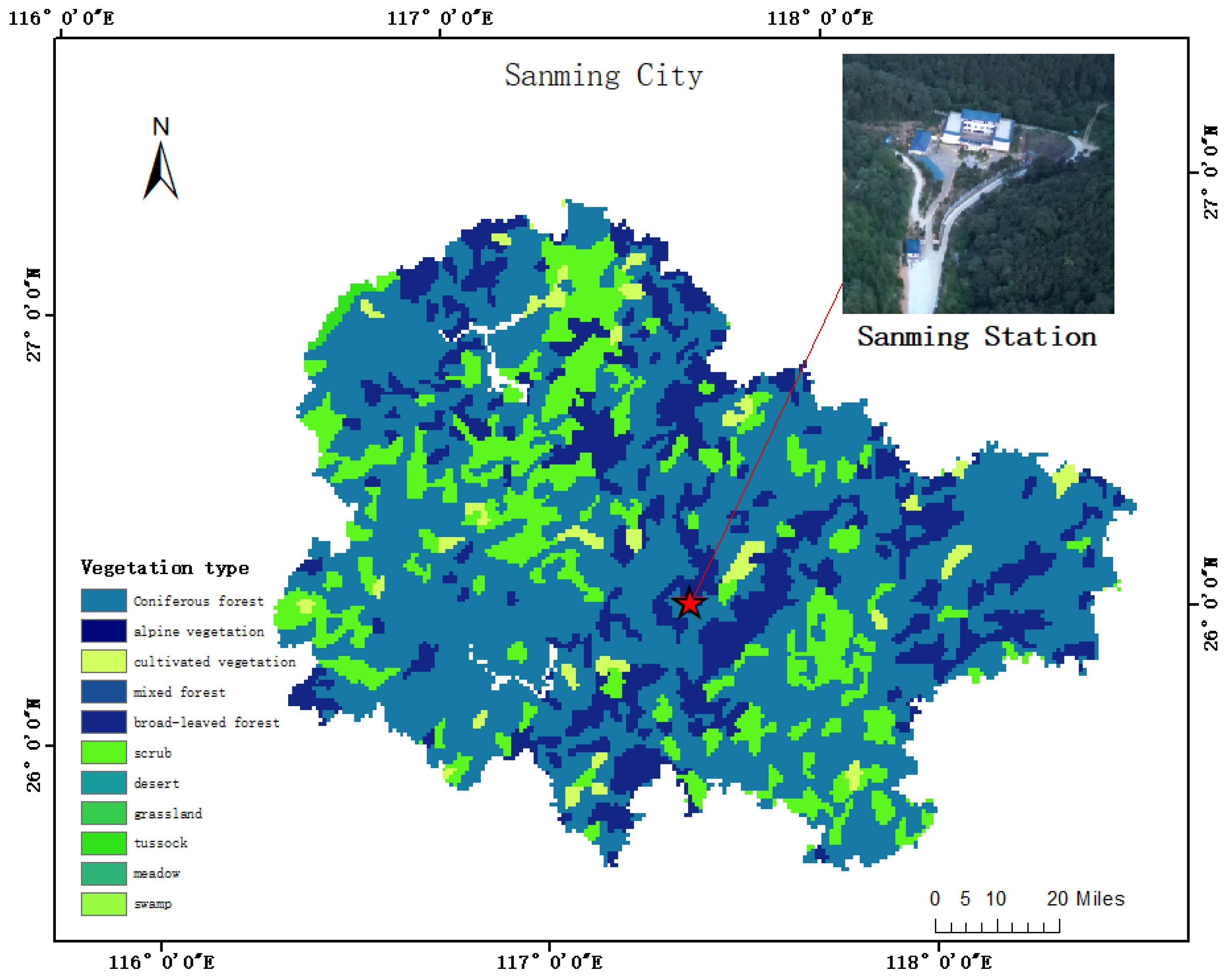
2.1. Study Area

The study area is located in Sanming City, Fujian Province, China. Fujian Province is one of China’s first comprehensive pilot zones for ecological civilization, boasting the country’s largest forest coverage. Sanming, located in southeastern China, is the largest nature reserve in Fujian and the country’s most extensive evergreen broad-leaved forest area [41]. Sanming city experiences an average annual precipitation of 1600–1900 mm, with the majority of rainfall occurring between April and September. The average annual temperature ranges from 18 °C to 20 °C, with winter temperatures (in January) averaging between 6 °C and 10 °C, and summer temperatures (in July) ranging from 27 °C to 30 °C, resulting in an overall warm and humid climate. According to the Köppen climate classification, Sanming is categorized as CFA (Humid Subtropical Climate), characterized by abundant rainfall throughout the year. It is also the core region for Chinese fir plantations and one of the most influential regions for species protection in China. The Sanming Field Experiment Station, established in 2004, serves as an experimental site for forest ecosystems and environmental studies (Figure 1).

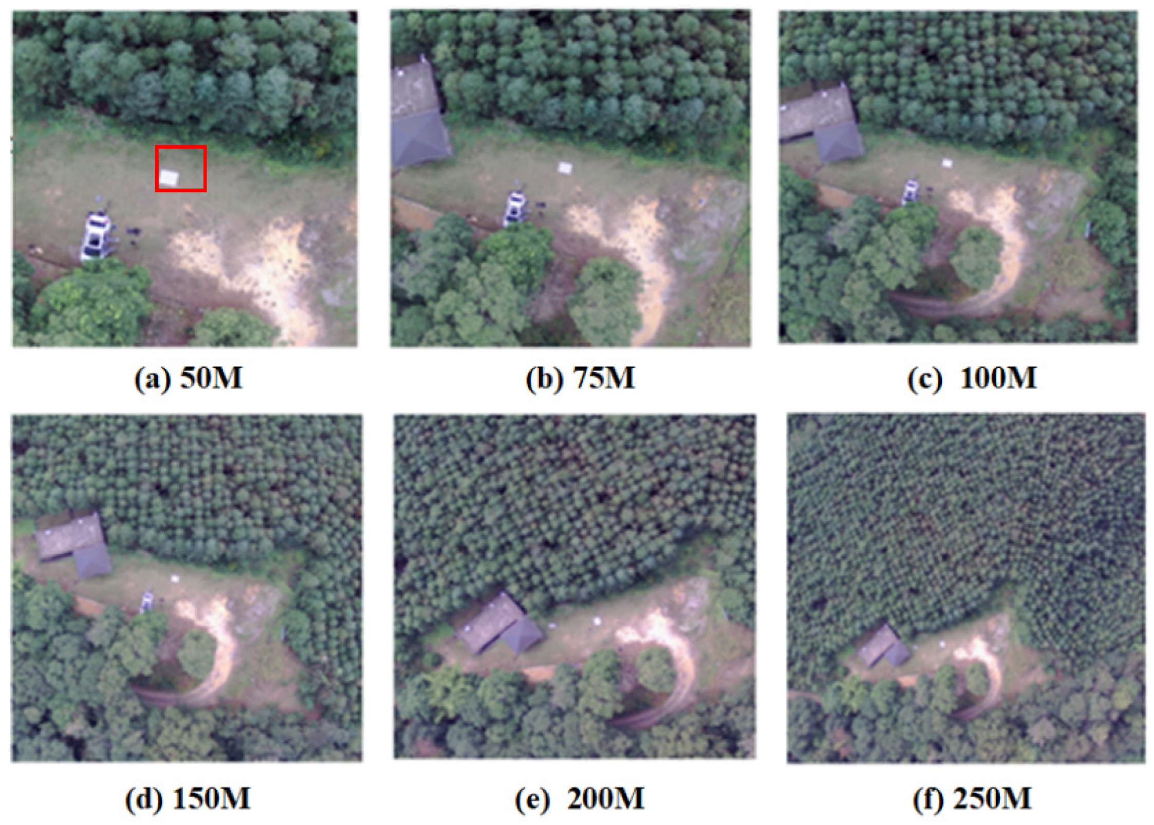
2.2. UAV Hyperspectral Image Acquisition

The UAV system used in this study was a DJI M600 Pro hexacopter drone (SZ DJI Technology Co., Ltd., Shenzhen, China) equipped with a GaiaSky-mini2-VN hyperspectral imaging system (Zolix Instruments Co., Ltd., Beijing, China). The M600 Pro features a professional A3 Pro flight control system integrated with three sets of Inertial Measurement Units (IMUs) and a Global Navigation Satellite System (GNSS) module, which, through residual analysis and software, establishes a redundant navigation system with six channels. The module is installed with shock absorption treatment to ensure accurate data acquisition and stability during UAV flights.
The GaiaSky-mini2-VN hyperspectral imaging system utilizes intra-pushbroom imaging technology, capable of hyperspectral imaging in the 388.9–1016.5 nm band (with 726 bands), featuring a resolution of 3.5 nm. It has a 27.3° field of view and an 18.5 mm focal length, making it suitable for detailed hyperspectral imaging in this spectral range.
The hyperspectral images used were acquired on 15 November 2023, at Sanming Station. To ensure stable weather conditions with minimal cloud cover, data acquisition was conducted on a day with favorable weather stability. The specific details of the UAV flying missions are shown in Table 1.
Before the UAV took off, the hyperspectral sensor was calibrated against a white reference panel to measure the digital number (DN) values of the panel, which served as a reference for solar irradiance intensity. According to this irradiance intensity, the optimal integration time for the sensor was calculated to capture high DN values, without exceeding its upper limit. Images of the forest canopy were collected from the nadir view at varying flight altitudes by flying the UAV in a directly ascending direction (Figure 2) to assess the differences in reflectance obtained from atmospheric correction using a grey panel at corresponding flight altitudes, compared to those using a single-altitude grey panel. Similarly, after collecting forest canopy images, the UAV flew above the grey panel and a series of flights at multiple altitudes was conducted by flying the UAV at a descending altitude to acquire hyperspectral imagery of the grey reference panel at various spatial resolutions (Table 2).

2.3. Data Processing

Preprocessing of the hyperspectral imagery was performed using SpecView 2.9 software, including lens correction, reflectance calculation, and atmospheric correction. Reflectance was calculated as the DN values of the image divided by the DN values of the white reference.
Due to the significant variation in UAV flight altitudes, the impact of atmospheric effects on the canopy reflectance is considerable. Therefore, selecting an appropriate atmospheric correction approach is essential to restore the true characteristics of the image. However, a mature method for atmospheric correction of UAV hyperspectral images of varying flight altitudes is currently lacking [45,46]. Accurate atmospheric parameters, such as water vapor content and aerosol distribution, are critical inputs for utilizing physical-based atmospheric correction algorithms to process hyperspectral images. However, these parameters are difficult to obtain over small altitude ranges, which limits the performance of the physical method for atmospheric correction of UAV hyperspectral images. We utilized the physical-based atmospheric correction function embedded in SpecView software to pre-correct the raw data, but also tested two different strategies with grey reference for atmospheric correction. One used the reflectance of the grey panel acquired at a single flight height (i.e., 250 m in this case), and the other used the reflectance of the grey panel acquired at the corresponding flight height (i.e., the grey reference obtained at the same height as the one to be corrected) to process post-atmospheric correction. The principle of atmospheric correction using the grey panel, which has wavelength-specific standard reflectance, was in the image as a reference.
R c o r r R m e a s = R s t a n d a r d R g r e y r e f
where Rcorrrefers to the reflectance after image correction, Rmeas is the measured reflectance of the image, Rstandard is the standard reflectance of the reference panel, and Rgreyref is the measured reflectance of the grey panel. During the process of atmospheric correction, the target and grey reference panel are assumed to be affected similarly by atmospheric conditions. The target wavelength-specific reflectance can be obtained from the measured reflectance of the target multiplied by the ratio of the standard reflectance to the measured reflectance of the grey panel.
Sample images from different flight altitudes are presented in Figure 3.
To investigate the effects of scale, it is necessary to control variables by delineating a fixed forest area at different altitudes, ensuring that the same target area is captured at each altitude. Thus, a fixed region was selected (Figure 4). To maintain consistency in canopy area across images captured at varying altitudes, the corresponding pixel count was calculated based on the spatial resolution at each altitude. Using the Region of Interest (ROI) tool in ENVI 5.0, canopy reflectance was extracted for the fixed forest area according to the calculated pixel count.
To analyze the impact of different observation altitudes on quantitative remote sensing of vegetation, we calculated four widely used indices at each altitude: the Normalized Difference Vegetation Index (NDVI) [47,48,49,50], Enhanced Vegetation Index (EVI) [51,52,53,54], Photochemical Reflectance Index (PRI) [55,56,57], and Chlorophyll Index Red Edge (CIRE) [58], using Equations (2)–(5):
N D V I = R 800 R 670 R 800 + R 670
E V I = 2.5 × R 800 R 680 R 800 + 6 × R 680 7.5 × R 480 + 1
P R I = R 531 R 570 R 531 + R 570
C I R E = R 740 / R 720 1
where the subscript numbers represent the corresponding wavelengths. Two different kinds of Vis’ ensembles are calculated: one is the same as shown in Figure 3, to calculate VIs of the same size image of vegetation for all flight heights, and the other is that shown in Figure 4, of the same area of forest canopy obtained from different altitudes.

3. Results

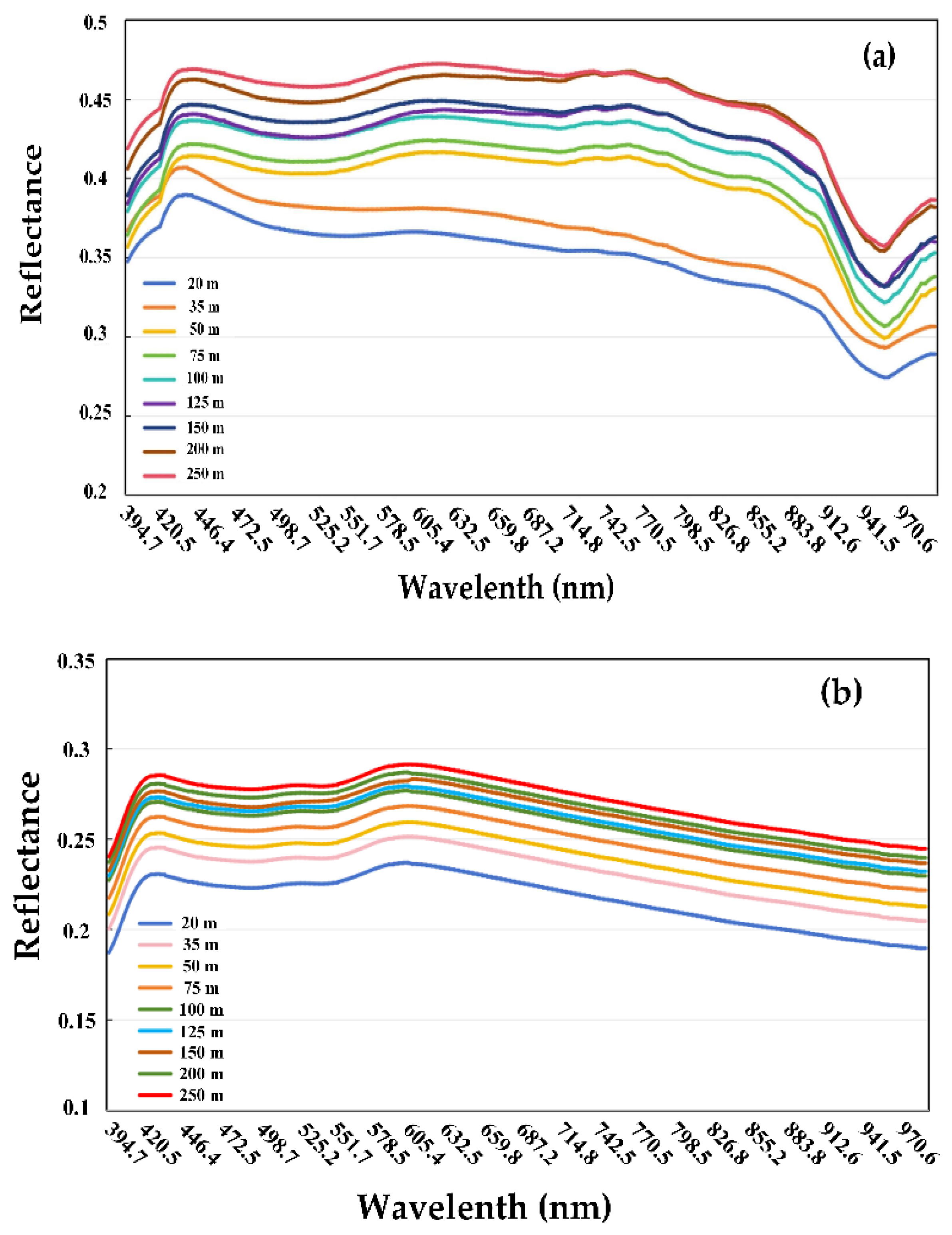
3.1. Atmospheric Correction Methods on Reflectance with Grey Reference

First, we use the reflectance correction results of the grey panel as an indicator of the effectiveness of the atmospheric correction. As displayed in Figure 5a, it is evident that the reflectance of the grey panels undergoes considerable variation from the visible to the near-infrared spectrum due to atmospheric effects. Therefore, effective atmospheric correction is essential for minimizing atmospheric interference in UAV-based hyperspectral imagery. After applying atmospheric correction using the reflectance of the grey panel acquired at a single flight height (i.e., 250 m), the reflectance of the grey panel yields a smooth curve, yet differences in reflectance across altitudes remain (Figure 5b). The variation of the reflectance follows the same pattern across altitudes as the uncorrected grey panel reflectance. With atmospheric correction using the reflectance of the grey panel acquired at the corresponding flight height (i.e., the grey reference obtained at the same height as the one to be corrected), all the reflectance of grey panels is successfully corrected to match the standard reflectance (Figure 5c), indicating that, to effectively correct atmospheric influence on UAV-based land surface reflectance, grey panel reflectance obtained from the corresponding flight height is mandatory.
For atmospheric correction on vegetation canopy reflectance, we also tested two strategies, using a single-altitude grey panel and the corresponding-altitude grey panel for reflectance correction. As shown in Figure 6, in visible bands, regardless of changes in flight altitude and atmospheric correction methods, reflectance does not show significant variation. While, the impact of different UAV flight heights on vegetation reflectance is primarily evident in the near-infrared region, and as the flight altitude increases, canopy reflectance gradually decreases. This may be due to the complex structure of the forest canopy, which causes stronger scattering effects in the near-infrared bands [59]. Moreover, as flight height increases, the reflected radiance of the canopy reaching the sensor is also affected by changes in the viewer geometry.
Figure 6a presents the average reflectance of the forest canopy at different heights after atmospheric correction with a grey panel at the same altitude (i.e., 20 m in this case). The significant differences in canopy reflectance in near-infrared bands across all the flying altitudes are partially due to the fact that using a single-altitude grey panel for correction of different flight height images cannot fully eliminate the atmospheric effects. When using the corresponding altitude grey panel for atmospheric correction (Figure 6b), significant differences still exist in canopy reflectance at the near-infrared region of low flight heights, but after reaching a certain altitude (>100 m), the forest canopy reflectance becomes nearly constant. This suggests that using a grey panel at the corresponding altitude for atmospheric correction of UAV-based imagery can effectively eliminate atmospheric effects, and there is possibly no need for extra atmospheric correction algorithms for preprocessing of UAV images.
The variation of near-inferred reflectance remaining for those low flight heights (<100 m, Figure 6b) is possibly due to viewer geometry and observed canopy heterogeneity. Once a certain height is reached, the canopy heterogeneity in the field of view of the sensor gradually diminishes [60], becoming negligible. As a result, when the flight altitude exceeds 100 m, the reflectance in all spectral bands of the forest canopy becomes almost indistinguishable.

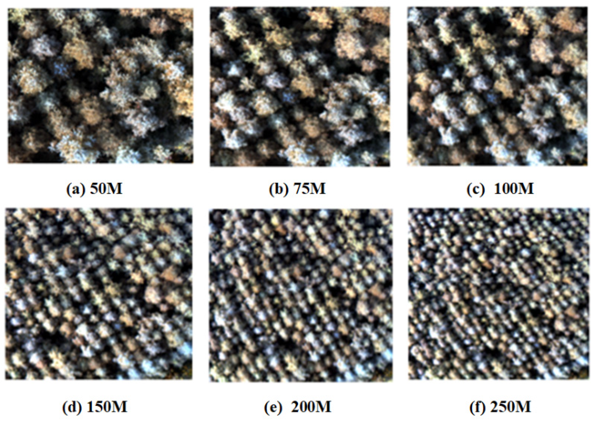
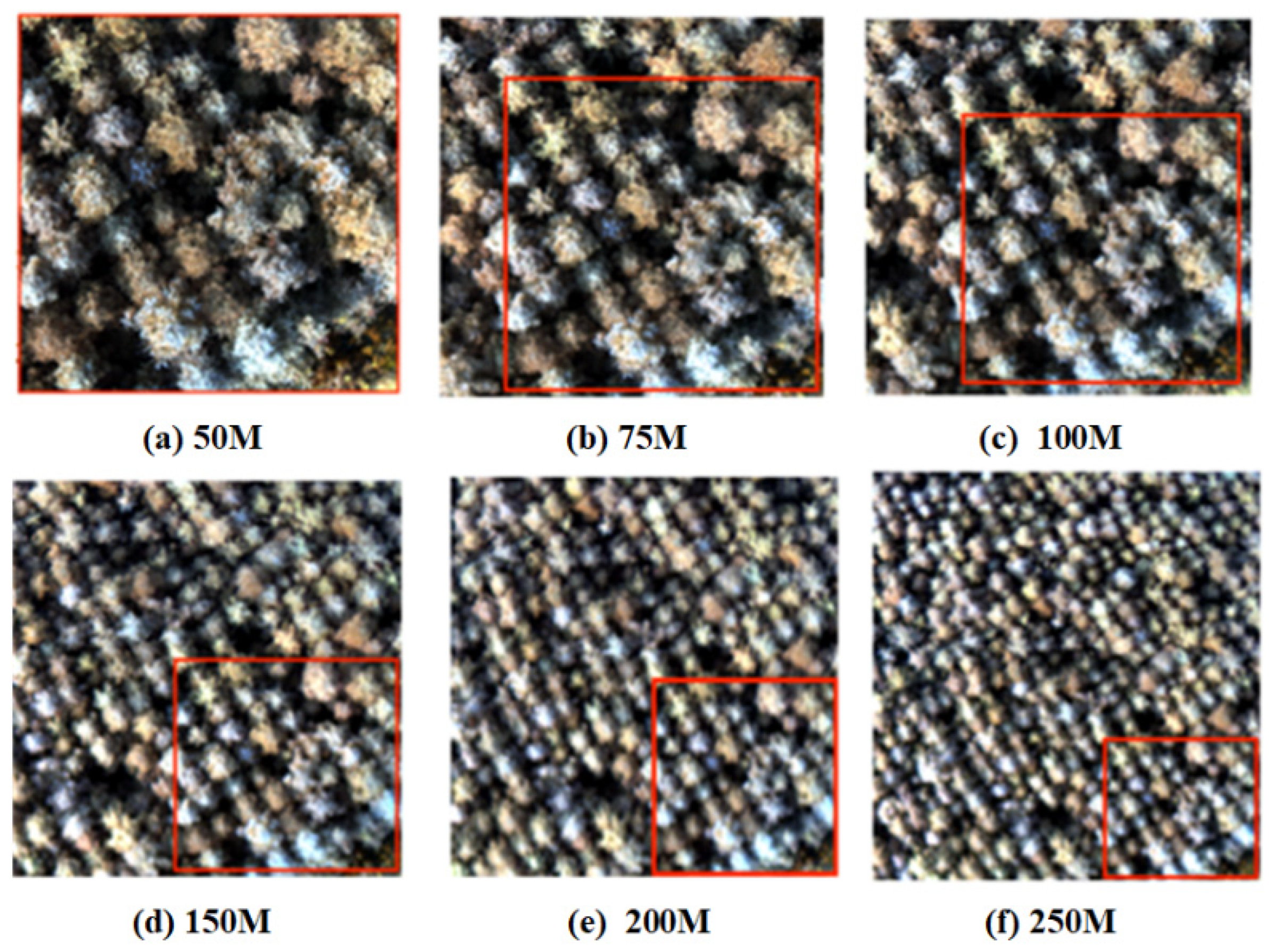
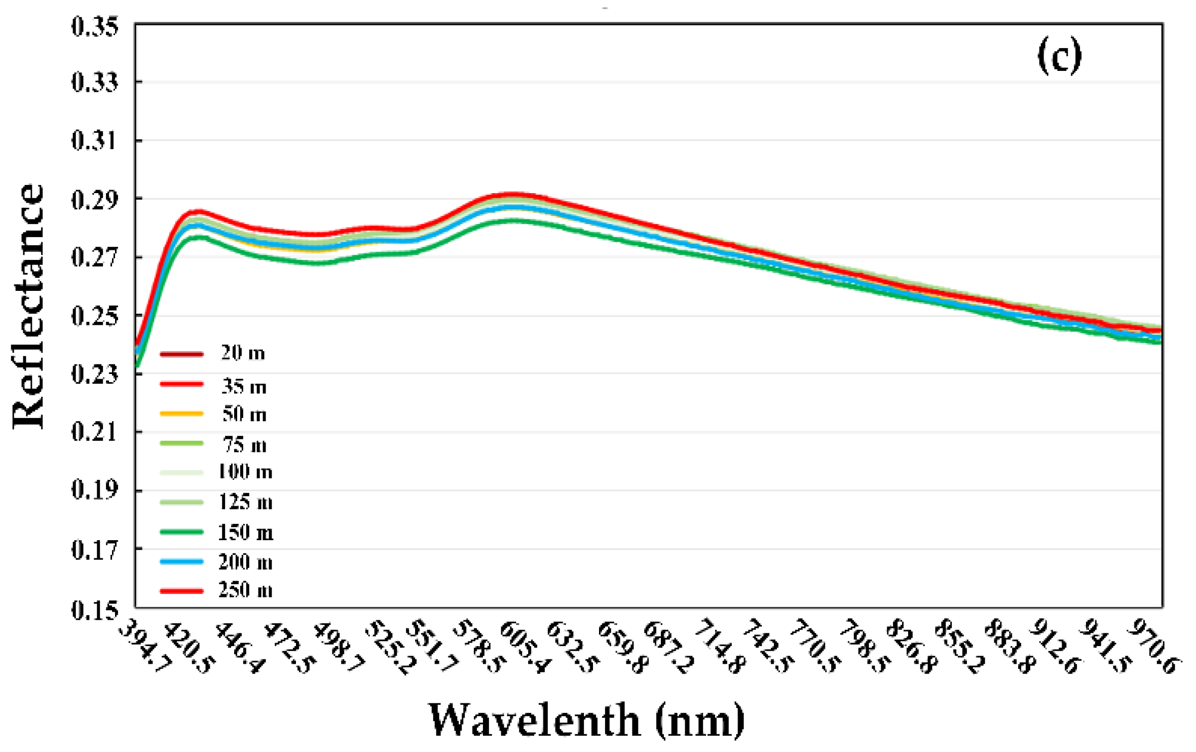
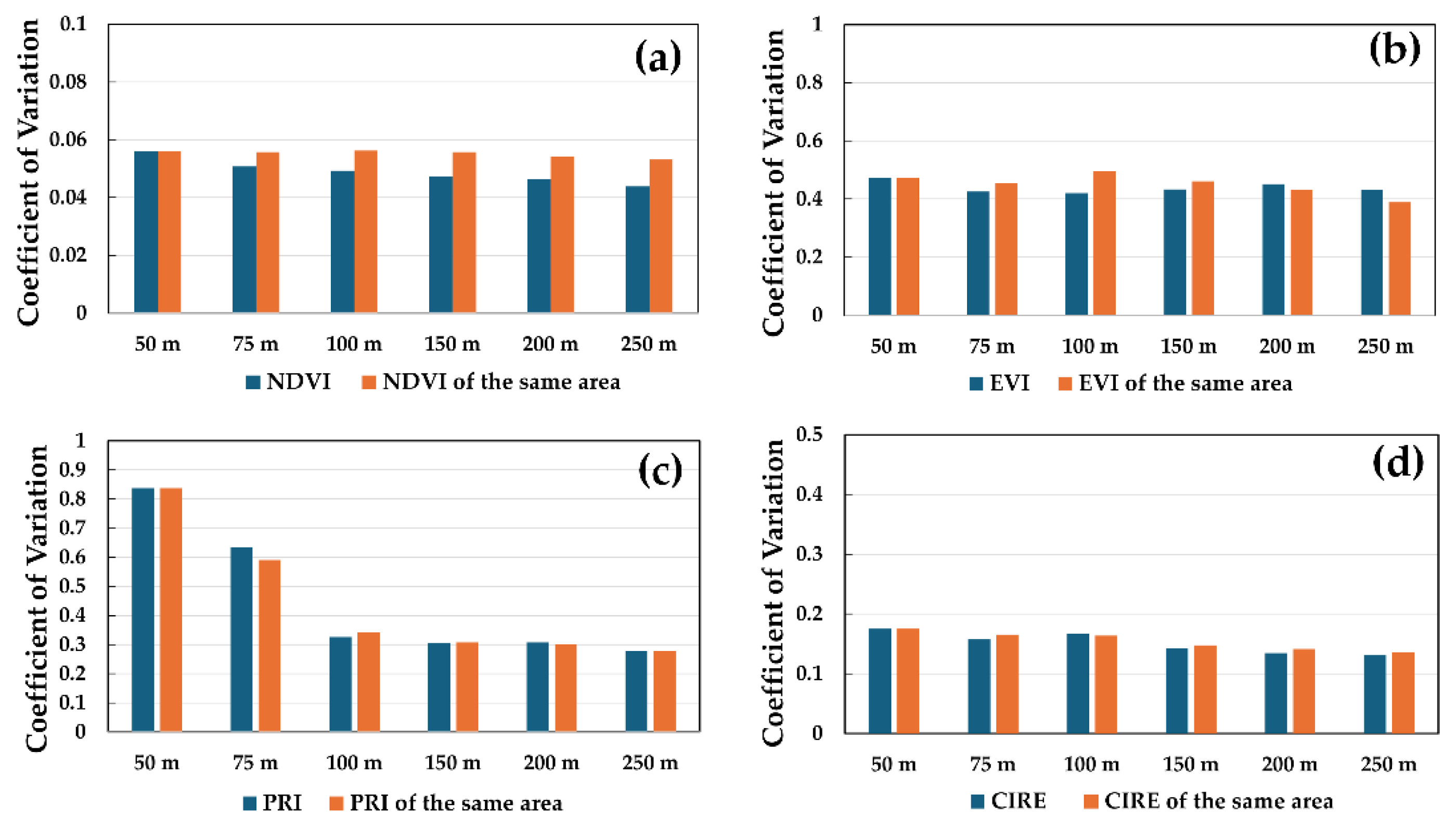
3.2. Impact of Observed Canopy Heterogeneity on Remote Sensing of Forest Canopy

As canopy reflectance still has significant variation at low altitudes, even after atmospheric correction (Figure 6b), we then investigated how vegetation indices change across altitudes. Figure 7 presents four vegetation indices. NDVI and EVI are commonly used vegetation indices that quantify vegetation cover and growth conditions. PRI assesses the pigment status of xanthophyll, while CIRE indicates chlorophyll content. Each flight altitude corresponds to a different spatial resolution, with resolution decreasing as altitude increases, resulting in each pixel representing a larger vegetation area. Different resolutions can thus present varying degrees of vegetation coverage and growth conditions. Images at different resolutions may display varying degrees of vegetation cover and growth conditions. In the high-resolution images (50 m height), finer structural details and variations in vegetation are visible. In the lower resolution images (250 m height), vegetation coverage may appear in a coarser representation. The distribution of vegetation indices at different flight altitudes is essentially consistent, while as the flight altitude increases, the clarity gradually decreases, with increasing coverage.
To quantitatively assess the impact of canopy heterogeneity on vegetation indices, the means and standard deviations of NDVI, PRI, CIRE, and EVI were calculated (Figure 8). Variations of the reflectance of related bands are also displayed in Figure 8a,b. It can be observed that NDVI exhibits significant changes from 50 m to 100 m (Figure 8b), as the reflectance at 800 nm varies greatly as well, while the reflectance at 670 nm shows minimal variation. The observed heterogeneity of the forest canopy at low altitudes, with its complex structure and strong scattering of near-infrared bands, contributes to these significant changes in reflectance and further NDVI. Beyond 100 m, the variation in NDVI remains marginal, with a stable standard deviation, as reflected by the stability in reflectance at 670 nm and 800 nm between 100 m and 250 m. Similarly, EVI shows more notable variation from 50 m and 100 m (Figure 8d), attributed to the significant decline in the reflectance at 800 nm, with little change in reflectance at 480 nm and 680 nm between 50 m and 100 m (Figure 8a,b). Since the flight height is above 100 m, the average standard deviation of EVI slightly decreases, but is more stable compared to that of NDVI.
PRI shows a notable increase, with a decreased standard deviation, when flight height increases from 75 m to 100 m (Figure 8e). However, the reflectance at 531 nm and 570 nm, which determine changes in PRI, showed few changes from 50 m to 250 m (Figure 8a,b). Considering that PRI is strongly affected by canopy structure and viewer geometry [61], the changes in PRI with increasing altitude could be partially due to changes in the heterogeneity of the image and the proportion of canopy shadows and soil background. The stability of PRI averages and reducing standard deviation from 100 m to 250 m suggests a stabilization of observed canopy heterogeneity and forest canopy proportions in the imagery.
As displayed in Figure 8e, CIRE showed a strong decline between 50 m and 100 m and stabilized after 100 m, while the standard deviation of CIRE kept gradually decreasing from 50 m to 250 m. The reflectance at 720 nm did not change much between 50 m and 100 m, but the reflectance at 740 nm varied significantly, leading to substantial changes between 50 m and 100 m (Figure 8a,b).

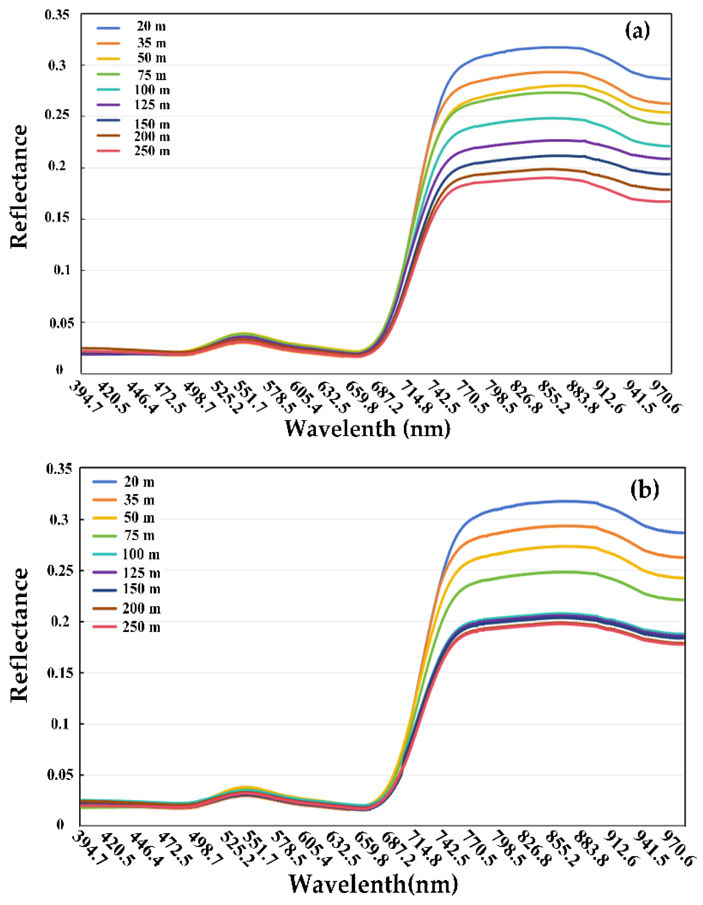
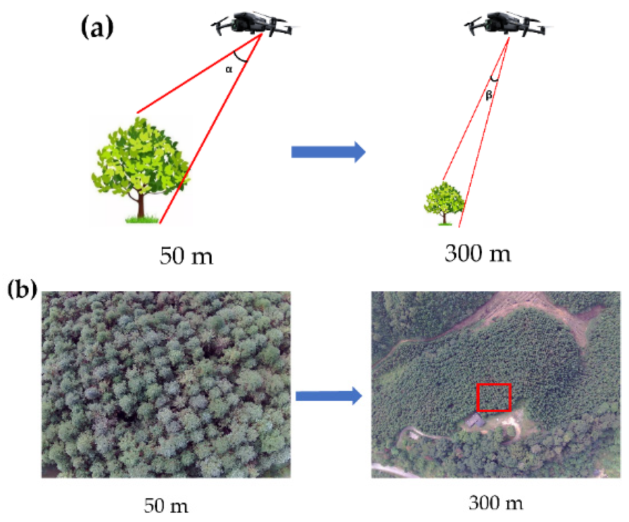
3.3. Impact of Viewer Geometry on Vegetation Indices of Forest Canopy

Figure 9 presents the mean and standard deviation of NDVI, PRI, CIRE, and EVI in the same area at various altitudes, indicating that the canopy heterogeneity is the same in this area but the viewer geometry changes across the altitudes. The variation trends of the NDVI, EVI, PRI and CIRE in the same area all exhibited similar patterns to those shown in Figure 8c–f, but with slight differences in absolute values. Generally, the standard deviations of the four indices for the same area were slightly higher than those for the whole image, and the decreasing trend of all the standard deviations with increasing altitudes was gentler. NDVI had smaller means but higher standard deviations for the same area (Figure 9a) compared to the whole image (Figure 8c). EVI displayed consistently relatively higher means and standard deviations, especially when altitudes were above 100 m, than those shown in Figure 8d. Both PRI and CIRE for the same area (Figure 9c,d) were more variable, with higher standard deviations at lower altitudes, relative to those for the whole image (Figure 8e,f). Considering the observed canopy heterogeneity of the same area is fixed for different flight heights, these changes are mainly attributed to the viewer geometry.
Figure 10 displays the coefficients of variation (CV) of the four VIs derived from the same size image and the same area as shown in Figure 8 and Figure 9, respectively. The different CVs of NDVI and EVI derived from the two kinds of images explain the differences between the results shown in Figure 8c,d and those shown in Figure 9a,b, implying the opposite influences of canopy heterogeneity versus viewer geometry on NDVI and EVI. The most variable CVs of PRI illustrate that PRI is very sensitive to flight altitude, due to the effects of viewer geometry. Relatively low and stable CVs of CIRE indicate the lowest influence of variant flight heights on CIRE among these four VIs. The overall declining trends of CVs of the four VIs across ascending flight heights demonstrate that higher flight altitudes generate relatively stable signals.

4. Discussion

In addition to close-range remote sensing, atmospheric correction is essential to process most spectral remote sensing data [62]. The scale effect is always coupled with atmospheric issues, as varying observation heights change both the scale and optical path length. The comparison of reflectance values before and after atmospheric correction demonstrated that atmospheric effects cause substantial variability in reflectance, particularly in the near-infrared bands. Crusiol et al. (2020) reported that different atmospheric calibration methods led to variations of near-infrared reflectance of up to 25% across different flight altitudes’ UAV imaging [63]. However, using the corresponding altitude calibration method reduced discrepancies in near-infrared bands to <3% (Figure 4c), emphasizing the utility of dynamic parameter adjustments for altitude-dependent atmospheric effects. Atmospheric correction significantly improved the smoothness of the reflectance, reducing the discrepancies caused by atmospheric scattering and absorption (Figure 5 and Figure 6). However, when the same single altitude grey reference panel was used for calibration of different flight heights, some discrepancies remained in the reflectance values (Figure 5b and Figure 6a). This indicates that, while this kind of atmospheric correction mitigates some of the atmospheric effects, the influences of atmospheric scattering and absorption cannot be entirely eliminated if the observation optical path lengths of the grey reference and the target are not the same. Another atmospheric correction method, which used the grey panel from the corresponding flight height, produced more consistent reflectance across all altitudes, demonstrating a more successful correction process. Even though UAV-based remote sensing is usually conducted at near-surface altitudes, and the atmospheric scattering and absorption is strong at this range [64,65,66], it is recommended to proceed with atmospheric correction using the grey reference acquired from the same optical path length, especially for observations of multiple altitudes of viewing angles. In addition, no extra physical-based models are needed to reduce the impact of atmospheric scattering and absorption, thus providing a simple but effective method to produce reliable vegetation index retrievals from hyperspectral data.
After effective atmospheric correction, the variation in reflectance across different flight altitudes is still significant, particularly in the near-infrared region at low altitudes (Figure 6a,b), but stabilizes when the flight height is above 100 m. This can be attributed to the complex structure of the forest canopy and its strong multiple scattering effect in near-infrared bands, which becomes more pronounced at lower flight altitudes due to the observed denser and more heterogeneous nature of the canopy [67,68,69]. As the UAV ascends to higher altitudes, the scattering effect decreases, and the canopy’s structural heterogeneity has a diminishing influence on the observed reflectance. The reflectance in the visible region showed minimal variation across altitudes, suggesting that the visible region is less sensitive to changes in altitude, possibly due to the relatively uniform scattering behavior of the canopy in these bands [70].
Changes in reflectance reflect the scale effects, which can be further explained by changes in viewer geometry and observed canopy heterogeneity with varying flight heights. Figure 11 illustrates how different flight heights affect viewer geometry and observed canopy heterogeneity. Viewer geometry refers to changes in the geometric characteristics of the same target observed at different scales, which can be also explained by the bidirectional reflectance distribution function (BRDF) effect of the canopy. When the flight altitude increases from 50 m to 300 m, the intersection angle for observing the tree changes from α to β, altering viewer geometry (Figure 11a). Meanwhile, the observed proportions of leaves and background also change and the observed canopy complexity is minimized, reducing the observed canopy heterogeneity. In addition to reflectance, changes in vegetation indices are also used to indirectly characterize scale effects.
In terms of vegetation indices, NDVI, EVI, PRI, and CIRE all displayed clear changes with altitude, especially at lower altitudes (Figure 7, Figure 8, Figure 9 and Figure 10). NDVI, EVI, and CIRE experienced obvious changes when flight height was below 100 m, reflecting the varying observed canopy heterogeneity and the influence of viewer geometry and canopy complexity. However, beyond 100 m, these indices showed stabilization, likely due to the reduction in the effect of observed canopy heterogeneity at higher altitudes. These findings are consistent with previous studies suggesting that vegetation indices are sensitive to both the spatial resolution of the imagery and the structural complexity of the vegetation being observed [71,72,73,74,75]. Additionally, the proportion of sunlit and shaded leaves and backgrounds within the field of view varies with different flight altitudes, contributing to changes in viewer geometry. As the altitude increases, the proportion of each component within the field of view tends to stabilize, reducing the impact of scale effects, and changes in reflectance and vegetation indices will gradually diminish. However, the higher the altitude of the UAV, the coarser the resolution data are, likely failing to capture fine-scale canopy heterogeneity, and leading to reduced precision of vegetation indices themselves and their effectiveness in vegetation monitoring, as with NDVI [76]. The results shown in Figure 7 reveal that NDVI and CIRE variations at 50–100 m altitudes (18% and 32% reduction in standard deviation, respectively) resolve sub-canopy structural details, highlighting the necessity of high-resolution data for heterogeneous ecosystems.
The standard deviation analysis of NDVI, PRI, CIRE, and EVI of the whole image revealed a gradual decrease with increasing altitude, suggesting stabilization of canopy shadows, soil background, and tree canopy components (Figure 8). At lower altitudes, the sensor is more likely to capture fine-scale variations in canopy structure, including variations in leaf density, shadow, and background soil, all of which contribute to the higher standard deviations observed for these indices. The standard deviation of PRI is at a high level and changes little between 50 m and 75 m, likely due to the relatively large proportions of canopy shadow and soil background in the imagery, as PRI is strongly affected by viewer geometry [70,77,78,79]. However, the slightly higher standard deviations in the same area compared to the entire image indicate that viewer geometry also has a significant impact (Figure 8 and Figure 9).
The viewer geometry influences canopy reflectance and vegetation index variability through the viewing angle and the distance from the canopy [78,80,81]. Zhang et al. (2021) demonstrated evident angular variations of several vegetation indices using multi-angle hyperspectral images, obtained using the same equipment as used in this study [82]. For nadir view observation, as the UAV flew at higher altitudes, the observed area increased, leading to a more spatially averaged representation of the forest canopy and a closer viewing angle for the pixels of the same target (Figure 9). This change in viewer geometry resulted in a reduction in the influence of fine-scale canopy heterogeneity, thereby contributing to the observed stabilization of vegetation indices at higher altitudes, which can be further supported by the declining CVs of Vis, as demonstrated by the results shown in Figure 10. While the observed canopy heterogeneity becomes less with increasing flight heights, the persistent variations in vegetation indices highlight the need for advanced image processing techniques to correct these effects and improve the accuracy of vegetation monitoring [83,84,85,86,87].
UAV-based hyperspectral imaging can provide valuable insights into vegetation structure and health, but the sensitivity of vegetation indices to atmospheric conditions and scale effects, including observed canopy heterogeneity and viewer geometry, requires careful calibration and processing to ensure accurate and reliable results. Poley et al. (2020) identified that lower flight heights performed better in biomass estimation [88]. In practical terms, for studies focusing on fine-scale vegetation structure and variability, lower altitudes (around 50 m to 100 m) may be preferred, as they capture more detailed canopy characteristics. Previous studies have suggested flying below 50 m to maximize spatial detail but overlooked scale-induced noise from canopy shadows and soil background [89,90]. For large-scale vegetation monitoring or studies that require stable index values for similar land surfaces, higher altitudes (above 100 m) may be more appropriate, as they reduce the influence of scale effects. However, even at higher altitudes, minor variations due to viewer geometry cannot be ignored. Our findings reconcile this trade-off by identifying 100 m as an optimal altitude, balancing spatial resolution and data reliability, aligning with a study on rice phenotyping, where altitudes >100 m provided generally stable signals [91].
Moreover, altitude-specific atmospheric correction should be employed to minimize atmospheric distortions and improve the accuracy of vegetation index calculations. However, acquisition of grey panels complicates field operations, especially in inaccessible or complex terrains, which means that more tests should be run for different targets to establish suitable measures. Developing machine learning models trained on multi-altitude data to predict atmospheric absorption without reliance on reference panels is also a possible option. This study focused on Chinese fir plantations in a single geographic region and season. Results may not generalize to other vegetation types with more complex canopy structures (e.g., natural secondary forest) or account for seasonal variations (e.g., leaf phenology, weather). The findings should be assessed across diverse ecosystems and seasons for broader applicability. Incorporating temporal analysis to evaluate scale effects under varying phenological stages or climatic conditions is of great interest. To better understand scale effects, multi-altitude hyperspectral data could be combined with multi-angle imaging to mitigate the impacts of viewer geometry and canopy heterogeneity on vegetation signals through, for example, downscaling a canopy-level signal to a leaf-level signal using geometric–optical models [92]. The application of a UAV-based platform to remote sensing of vegetation needs to optimize UAV flight plans to balance the requirements of detailed spatial information and stabilized reflectance and vegetation indices, as well as reducing atmospheric influences. Future research should further explore the optimal flight altitudes and atmospheric correction strategies for various vegetation types and monitoring objectives, to enhance the accuracy and reliability of UAV-based remote sensing applications.

5. Conclusions

This study aimed to investigate the impact of scale effect on remote sensing of vegetation using UAV-based hyperspectral imagery obtained from varying flight altitudes. The variations in canopy reflectance and vegetation indices across different altitudes emphasize the intricate relationship between atmospheric effects, viewer geometry, and the structural characteristics of the forest canopy. The findings contribute to the understanding of scale effects in remote sensing and provide insights into the optimal use of UAV technology for vegetation monitoring.
Atmospheric correction of UAV-based hyperspectral imagery is essential for accurate reflectance and vegetation index retrieval. The method of using a grey reference panel corresponding to the flight altitude for atmospheric correction yields better results compared to using a grey reference panel at a constant height. This altitude-specific calibration effectively mitigates atmospheric distortions and enhances the accuracy of the reflectance values across different altitudes, reducing discrepancies in near-infrared bands from 15% to <3%.
The reflectance in the near-infrared bands is significantly affected by observed canopy heterogeneity, which varies with changes in the UAV’s collection height. Consequently, the variation in some vegetation indices across the entire image is greatly influenced by the same factor, in other words, by mixed pixels. The results show that NDVI increased by 18% between 50 m and 75 m, and the standard deviation decreased by 32% from 50 m to 250 m. An appropriate UAV hyperspectral acquisition height can eliminate reflectance differences in the near-infrared bands of vegetation. Above an altitude of 100 m, the observed heterogeneity of the forest canopy is mitigated, and its impact on the near-infrared bands is weakened. The remaining variation in vegetation indices of the same area of images is also influenced by the viewer geometry. Viewer geometry can cause the shape and position of targets to appear differently in the imagery, affecting reflectance changes and variations of vegetation indices. PRI variability from 50 to 75 m (in which means almost tripled, from 0.03 to 0.08), linked to viewer geometry, highlighted the need for multi-angle corrections. These findings amplify the inherent compromises of UAV missions between spatial detail, coverage area, and time efficiency. For forest observations, 50 m flights resolve finer canopy structures (e.g., leaf clumping, leaf area), but these flights may take four times longer than flying at 150 m, increasing operational costs and weather dependency. However, 150 m flights sacrifice detail but achieve rapid coverage, which is ideal for regional carbon stock assessments. This suggests that low altitudes should be used for precision monitoring, like disease/pest detection (high resolution) and higher altitudes for efficient and stable VIs retrieval (low noise).
In summary, this study highlights the importance of altitude-specific atmospheric correction, and the influence of scale effects on remote sensing of vegetation from the perspectives of observed canopy heterogeneity and viewer geometry. These findings provide valuable insights into optimizing UAV-based hyperspectral remote sensing for forest canopy monitoring, ensuring more accurate and reliable vegetation assessments.

Author Contributions

Conceptualization, F.Q., X.Z. and Q.Z.; methodology, H.Z. and Q.Z.; software, T.W.; formal analysis, T.W. and T.G.; data curation, H.Z. and Q.Z.; writing—original draft preparation, T.W. and T.G.; writing—review and editing, F.Q., L.L. and Q.Z.; funding acquisition, F.Q., X.Z. and Q.Z. All authors have read and agreed to the published version of the manuscript.

Funding

This research was funded by the National Natural Science Foundation of China, grant number 42071392, 42071050, the Open Fund of State Key Laboratory of Remote Sensing Science, grant number OFSLRSS202315, the Taishan Scholar project, and the Open Foundation of Scientific Observation and Research Station for Ecological Environment of Wuyi Mountains.

Data Availability Statement

The data that support the findings of this study are available from the corresponding author upon reasonable request.

Acknowledgments

We gratefully acknowledge all the support from the Sanming station for conducting UAV observation. We further acknowledge Zhiqiang Cheng (Fujian Normal University, China) for his support in instrumental assistance in data acquisition and processing. Many thanks to three anonymous reviewers who provided helpful comments to the improvement of the manuscript.

Conflicts of Interest

The authors declare no conflicts of interest.

References

  1. Karteris, M.; Theodoridou, I.; Mallinis, G.; Tsiros, E.; Karteris, A. Towards a green sustainable strategy for Mediterranean cities: Assessing the benefits of large-scale green roofs implementation in Thessaloniki, Northern Greece, using environmental modelling, GIS and very high spatial resolution remote sensing data. Renew. Sustain. Energy Rev. 2016, 58, 510–525. [Google Scholar] [CrossRef]
  2. Cao, C.; Lam, N.S.-N. Understanding the scale and resolution effects in remote sensing and GIS. In Scale in Remote Sensing and GIS; Routledge: London, UK, 2023; pp. 57–72. [Google Scholar]
  3. Zhu, Q.; Guo, X.; Deng, W.; Shi, S.; Guan, Q.; Zhong, Y.; Zhang, L.; Li, D. Land-use/land-cover change detection based on a Siamese global learning framework for high spatial resolution remote sensing imagery. ISPRS J. Photogramm. Remote Sens. 2022, 184, 63–78. [Google Scholar] [CrossRef]
  4. Peng, D.; Zhang, X.; Zhang, B.; Liu, L.; Liu, X.; Huete, A.R.; Huang, W.; Wang, S.; Luo, S.; Zhang, X.; et al. Scaling effects on spring phenology detections from MODIS data at multiple spatial resolutions over the contiguous United States. ISPRS J. Photogramm. Remote Sens. 2017, 132, 185–198. [Google Scholar] [CrossRef]
  5. Woodcock, C.E.; Strahler, A.H. The factor of scale in remote sensing. Remote Sens. Environ. 1987, 21, 311–332. [Google Scholar] [CrossRef]
  6. Wen, D.; Huang, X.; Bovolo, F.; Li, J.; Ke, X.; Zhang, A.; Benediktsson, J.A. Change detection from very-high-spatial-resolution optical remote sensing images: Methods, applications, and future directions. IEEE Geosci. Remote Sens. Mag. 2021, 9, 68–101. [Google Scholar] [CrossRef]
  7. Hengl, T. Finding the right pixel size. Comput. Geosci. 2006, 32, 1283–1298. [Google Scholar] [CrossRef]
  8. Tian, Y.; Wu, Z.; Li, M.; Wang, B.; Zhang, X. Forest fire spread monitoring and vegetation dynamics detection based on multi-source remote sensing images. Remote Sens. 2022, 14, 4431. [Google Scholar] [CrossRef]
  9. You, Y.; Cao, J.; Zhou, W. A survey of change detection methods based on remote sensing images for multi-source and multi-objective scenarios. Remote Sens. 2020, 12, 2460. [Google Scholar] [CrossRef]
  10. Aasen, H.; Honkavaara, E.; Lucieer, A.; Zarco-Tejada, P.J. Quantitative remote sensing at ultra-high resolution with UAV spectroscopy: A review of sensor technology, measurement procedures, and data correction workflows. Remote Sens. 2018, 10, 1091. [Google Scholar] [CrossRef]
  11. Zhang, Z.; Zhu, L. A review on unmanned aerial vehicle remote sensing: Platforms, sensors, data processing methods, and applications. Drones 2023, 7, 398. [Google Scholar] [CrossRef]
  12. Yao, H.; Qin, R.; Chen, X. Unmanned aerial vehicle for remote sensing applications—A review. Remote Sens. 2019, 11, 1443. [Google Scholar] [CrossRef]
  13. Feng, L.; Chen, S.; Zhang, C.; Zhang, Y.; He, Y. A comprehensive review on recent applications of unmanned aerial vehicle remote sensing with various sensors for high-throughput plant phenotyping. Comput. Electron. Agric. 2021, 182, 106033. [Google Scholar] [CrossRef]
  14. Guimarães, N.; Pádua, L.; Marques, P.; Silva, N.; Peres, E.; Sousa, J.J. Forestry remote sensing from unmanned aerial vehicles: A review focusing on the data, processing and potentialities. Remote Sens. 2020, 12, 1046. [Google Scholar] [CrossRef]
  15. Iizuka, K.; Itoh, M.; Shiodera, S.; Matsubara, T.; Dohar, M.; Watanabe, K. Advantages of unmanned aerial vehicle (UAV) photogrammetry for landscape analysis compared with satellite data: A case study of postmining sites in Indonesia. Cogent Geosci. 2018, 4, 1498180. [Google Scholar] [CrossRef]
  16. Pajares, G. Overview and current status of remote sensing applications based on unmanned aerial vehicles (UAVs). Photogramm. Eng. Remote Sens. 2015, 81, 281–330. [Google Scholar] [CrossRef]
  17. Bhardwaj, A.; Sam, L.; Akanksha; Martín-Torres, F.J.; Kumar, R. UAVs as remote sensing platform in glaciology: Present applications and future prospects. Remote Sens. Environ. 2016, 175, 196–204. [Google Scholar] [CrossRef]
  18. Salamí, E.; Barrado, C.; Pastor, E. UAV flight experiments applied to the remote sensing of vegetated areas. Remote Sens. 2014, 6, 11051–11081. [Google Scholar] [CrossRef]
  19. Guo, Y.; Yin, G.; Sun, H.; Wang, H.; Chen, S.; Senthilnath, J.; Wang, J.; Fu, Y. Scaling effects on chlorophyll content estimations with RGB camera mounted on a UAV platform using machine-learning methods. Sensors 2020, 20, 5130. [Google Scholar] [CrossRef]
  20. Pascucci, S.; Pignatti, S.; Casa, R.; Darvishzadeh, R.; Huang, W. Special issue “hyperspectral remote sensing of agriculture and vegetation”. Remote Sens. 2020, 12, 3665. [Google Scholar] [CrossRef]
  21. Li, Z.; Guo, X. Remote sensing of terrestrial non-photosynthetic vegetation using hyperspectral, multispectral, SAR, and LiDAR data. Prog. Phys. Geogr. Earth Environ. 2016, 40, 276–304. [Google Scholar] [CrossRef]
  22. Hyperspectral Remote Sensing of Agriculture on JSTOR. Available online: https://www.jstor.org/stable/24216514 (accessed on 15 January 2025).
  23. Adão, T.; Hruška, J.; Pádua, L.; Bessa, J.; Peres, E.; Morais, R.; Sousa, J.J. Hyperspectral imaging: A review on UAV-based sensors, data processing and applications for agriculture and forestry. Remote Sens. 2017, 9, 1110. [Google Scholar] [CrossRef]
  24. Zhang, Y.; Migliavacca, M.; Penuelas, J.; Ju, W. Advances in hyperspectral remote sensing of vegetation traits and functions. Remote Sens. Environ. 2021, 252, 112121. [Google Scholar] [CrossRef]
  25. Thenkabail, P.S.; Lyon, J.G.; Huete, A. Advances in hyperspectral remote sensing of vegetation and agricultural crops. In Fundamentals, Sensor Systems, Spectral Libraries, and Data Mining for Vegetation; CRC Press: Boca Raton, FL, USA, 2018; pp. 3–37. [Google Scholar]
  26. Lu, B.; Dao, P.D.; Liu, J.; He, Y.; Shang, J. Recent advances of hyperspectral imaging technology and applications in agriculture. Remote Sens. 2020, 12, 2659. [Google Scholar] [CrossRef]
  27. Näsi, R.; Honkavaara, E.; Lyytikäinen-Saarenmaa, P.; Blomqvist, M.; Litkey, P.; Hakala, T.; Viljanen, N.; Kantola, T.; Tanhuanpää, T.; Holopainen, M. Using UAV-based photogrammetry and hyperspectral imaging for mapping bark beetle damage at tree-level. Remote Sens. 2015, 7, 15467–15493. [Google Scholar] [CrossRef]
  28. Cao, J.; Leng, W.; Liu, K.; Liu, L.; He, Z.; Zhu, Y. Object-based mangrove species classification using unmanned aerial vehicle hyperspectral images and digital surface models. Remote Sens. 2018, 10, 89. [Google Scholar] [CrossRef]
  29. Du, B.; Zhao, R.; Zhang, L.; Zhang, L. A spectral-spatial based local summation anomaly detection method for hyperspectral images. Signal Process. 2016, 124, 115–131. [Google Scholar] [CrossRef]
  30. Liu, T.; Gu, Y.; Chanussot, J.; Dalla Mura, M. Multimorphological superpixel model for hyperspectral image classification. IEEE Trans. Geosci. Remote Sens. 2017, 55, 6950–6963. [Google Scholar] [CrossRef]
  31. Akinyoola, J.A.; Oluleye, A.; Gbode, I.E. A Review of Atmospheric Aerosol Impacts on Regional Extreme Weather and Climate Events. Aerosol Sci. Eng. 2024, 8, 249–274. [Google Scholar] [CrossRef]
  32. Seinfeld, J.H.; Bretherton, C.; Carslaw, K.S.; Coe, H.; DeMott, P.J.; Dunlea, E.J.; Feingold, G.; Ghan, S.; Guenther, A.B.; Kahn, R.; et al. Improving our fundamental understanding of the role of aerosol−cloud interactions in the climate system. Proc. Natl. Acad. Sci. USA 2016, 113, 5781–5790. [Google Scholar] [CrossRef]
  33. Zhao, X.; Yang, G.; Liu, J.; Zhang, X.; Xu, B.; Wang, Y.; Zhao, C.; Gai, J. Estimation of soybean breeding yield based on optimization of spatial scale of UAV hyperspectral image. Trans. Chin. Soc. Agric. Eng. 2017, 33, 110–116. [Google Scholar]
  34. Comerón, A.; Muñoz-Porcar, C.; Rocadenbosch, F.; Rodríguez-Gómez, A.; Sicard, M. Current research in lidar technology used for the remote sensing of atmospheric aerosols. Sensors 2017, 17, 1450. [Google Scholar] [CrossRef]
  35. Archer-Nicholls, S.; Lowe, D.; Schultz, D.M.; McFiggans, G. Aerosol–radiation–cloud interactions in a regional coupled model: The effects of convective parameterisation and resolution. Atmos. Chem. Phys. 2016, 16, 5573–5594. [Google Scholar] [CrossRef]
  36. Lyu, X.; Li, X.; Dang, D.; Dou, H.; Wang, K.; Lou, A. Unmanned aerial vehicle (UAV) remote sensing in grassland ecosystem monitoring: A systematic review. Remote Sens. 2022, 14, 1096. [Google Scholar] [CrossRef]
  37. Sankey, T.T.; McVay, J.; Swetnam, T.L.; McClaran, M.P.; Heilman, P.; Nichols, M. UAV hyperspectral and lidar data and their fusion for arid and semi-arid land vegetation monitoring. Remote Sens. Ecol. Conserv. 2018, 4, 20–33. [Google Scholar] [CrossRef]
  38. Yan, Y.; Deng, L.; Liu, X.; Zhu, L. Application of UAV-based multi-angle hyperspectral remote sensing in fine vegetation classification. Remote Sens. 2019, 11, 2753. [Google Scholar] [CrossRef]
  39. Ma, Y.; Zhang, J.; Zhang, J. Analysis of Unmanned Aerial Vehicle (UAV) hyperspectral remote sensing monitoring key technology in coastal wetland. In Proceedings of the Selected Papers of the Photoelectronic Technology Committee Conferences held November 2015, Various, China, 15–28 November 2015; Volume 2016, pp. 721–729. [Google Scholar]
  40. Du, X.; Zhou, Z.; Huang, D. Influence of Spatial Scale Effect on UAV Remote Sensing Accuracy in Identifying Chinese Cabbage (Brassica rapa subsp. Pekinensis) Plants. Agriculture 2024, 14, 1871. [Google Scholar] [CrossRef]
  41. Ma, S.; Shao, X.; Xu, C. Landslides triggered by the 2016 heavy rainfall event in Sanming, Fujian Province: Distribution pattern analysis and spatio-temporal susceptibility assessment. Remote Sens. 2023, 15, 2738. [Google Scholar] [CrossRef]
  42. Wang, H.; Zhu, A.; Duan, A.; Wu, H.; Zhang, J. Responses to subtropical climate in radial growth and wood density of Chinese fir provenances, southern China. For. Ecol. Manag. 2022, 521, 120428. [Google Scholar] [CrossRef]
  43. Cao, S.; Duan, H.; Sun, Y.; Hu, R.; Wu, B.; Lin, J.; Deng, W.; Li, Y.; Zheng, H. Genome-wide association study with growth-related traits and secondary metabolite contents in red-and white-heart Chinese fir. Front. Plant Sci. 2022, 13, 922007. [Google Scholar] [CrossRef]
  44. Wang, H.; Sun, J.; Duan, A.; Zhu, A.; Wu, H.; Zhang, J. Dendroclimatological analysis of chinese fir using a long-term provenance trial in Southern China. Forests 2022, 13, 1348. [Google Scholar] [CrossRef]
  45. Yu, X.; Liu, Q.; Liu, X.; Liu, X.; Wang, Y. A physical-based atmospheric correction algorithm of unmanned aerial vehicles images and its utility analysis. Int. J. Remote Sens. 2017, 38, 3101–3112. [Google Scholar] [CrossRef]
  46. Schläpfer, D.; Popp, C.; Richter, R. Drone data atmospheric correction concept for multi-and hyperspectral imagery–the DROACOR model. Int. Arch. Photogramm. Remote Sens. Spat. Inf. Sci. 2020, XLIII-B3-2, 473–478. [Google Scholar] [CrossRef]
  47. Eisfelder, C.; Asam, S.; Hirner, A.; Reiners, P.; Holzwarth, S.; Bachmann, M.; Gessner, U.; Dietz, A.; Huth, J.; Bachofer, F.; et al. Seasonal Vegetation Trends for Europe over 30 Years from a Novel Normalised Difference Vegetation Index (NDVI) Time-Series—The TIMELINE NDVI Product. Remote Sens. 2023, 15, 3616. [Google Scholar] [CrossRef]
  48. Fan, X.; Liu, Y. Multisensor Normalized Difference Vegetation Index Intercalibration: A comprehensive overview of the causes of and solutions for multisensor differences. IEEE Geosci. Remote Sens. Mag. 2018, 6, 23–45. [Google Scholar] [CrossRef]
  49. Gopinath, G.; Ambili, G.K.; Gregory, S.J.; Anusha, C.K. Drought risk mapping of south-western state in the Indian peninsula—A web based application. J. Environ. Manag. 2015, 161, 453–459. [Google Scholar] [CrossRef] [PubMed]
  50. Song, B.; Park, K. Detection of aquatic plants using multispectral UAV imagery and vegetation index. Remote Sens. 2020, 12, 387. [Google Scholar] [CrossRef]
  51. Kong, D.; Zhang, Y.; Gu, X.; Wang, D. A robust method for reconstructing global MODIS EVI time series on the Google Earth Engine. ISPRS J. Photogramm. Remote Sens. 2019, 155, 13–24. [Google Scholar] [CrossRef]
  52. Alexandridis, T.K.; Ovakoglou, G.; Clevers, J.G.P.W. Relationship between MODIS EVI and LAI across time and space. Geocarto Int. 2020, 35, 1385–1399. [Google Scholar] [CrossRef]
  53. Wang, C.; Wu, Y.; Hu, Q.; Hu, J.; Chen, Y.; Lin, S.; Xie, Q. Comparison of vegetation phenology derived from solar-induced chlorophyll fluorescence and enhanced vegetation index, and their relationship with climatic limitations. Remote Sens. 2022, 14, 3018. [Google Scholar] [CrossRef]
  54. Shi, H.; Li, L.; Eamus, D.; Huete, A.; Cleverly, J.; Tian, X.; Yu, Q.; Wang, S.; Montagnani, L.; Magliulo, V.; et al. Assessing the ability of MODIS EVI to estimate terrestrial ecosystem gross primary production of multiple land cover types. Ecol. Indic. 2017, 72, 153–164. [Google Scholar] [CrossRef]
  55. Hikosaka, K.; Tsujimoto, K. Linking remote sensing parameters to CO2 assimilation rates at a leaf scale. J. Plant Res. 2021, 134, 695–711. [Google Scholar] [CrossRef] [PubMed]
  56. Sukhova, E.; Zolin, Y.; Popova, A.; Yudina, L.; Sukhov, V. The influence of soil salt stress on modified photochemical reflectance indices in pea plants. Remote Sens. 2023, 15, 3772. [Google Scholar] [CrossRef]
  57. Zhang, C.; Filella, I.; Garbulsky, M.F.; Peñuelas, J. Affecting factors and recent improvements of the photochemical reflectance index (PRI) for remotely sensing foliar, canopy and ecosystemic radiation-use efficiencies. Remote Sens. 2016, 8, 677. [Google Scholar] [CrossRef]
  58. Delegido, J.; Verrelst, J.; Meza, C.M.; Rivera, J.P.; Alonso, L.; Moreno, J. A red-edge spectral index for remote sensing estimation of green LAI over agroecosystems. Eur. J. Agron. 2013, 46, 42–52. [Google Scholar] [CrossRef]
  59. Kimes, D.S. Dynamics of directional reflectance factor distributions for vegetation canopies. Appl. Opt. 1983, 22, 1364–1372. [Google Scholar] [CrossRef]
  60. Asner, G.P. Biophysical and biochemical sources of variability in canopy reflectance. Remote Sens. Environ. 1998, 64, 234–253. [Google Scholar] [CrossRef]
  61. Hilker, T.; Hall, F.G.; Coops, N.C.; Lyapustin, A.; Wang, Y.; Nesic, Z.; Grant, N.; Black, T.A.; Wulder, M.A.; Kljun, N.; et al. Remote sensing of photosynthetic light-use efficiency across two forested biomes: Spatial scaling. Remote Sens. Environ. 2010, 114, 2863–2874. [Google Scholar] [CrossRef]
  62. Moravec, D.; Komárek, J.; López-Cuervo Medina, S.; Molina, I. Effect of atmospheric corrections on NDVI: Intercomparability of Landsat 8, Sentinel-2, and UAV sensors. Remote Sens. 2021, 13, 3550. [Google Scholar] [CrossRef]
  63. Crusiol, L.G.T.; Nanni, M.R.; Furlanetto, R.H.; Cezar, E.; Silva, G.F.C. Reflectance calibration of UAV-based visible and near-infrared digital images acquired under variant altitude and illumination conditions. Remote Sens. Appl. Soc. Environ. 2020, 18, 100312. [Google Scholar]
  64. Fahey, T.; Islam, M.; Gardi, A.; Sabatini, R. Laser beam atmospheric propagation modelling for aerospace LIDAR applications. Atmosphere 2021, 12, 918. [Google Scholar] [CrossRef]
  65. Stuhl, B.K. Atmospheric refraction corrections in ground-to-satellite optical time transfer. Opt. Express 2021, 29, 13706–13714. [Google Scholar] [CrossRef]
  66. Mobley, C.D.; Werdell, J.; Franz, B.; Ahmad, Z.; Bailey, S. Atmospheric Correction for Satellite Ocean Color Radiometry; No. GSFC-E-DAA-TN35509; NASA: Washington, DC, USA, 2016.
  67. van der Tol, C.; Vilfan, N.; Dauwe, D.; Cendrero-Mateo, M.P.; Yang, P. The scattering and re-absorption of red and near-infrared chlorophyll fluorescence in the models Fluspect and SCOPE. Remote Sens. Environ. 2019, 232, 111292. [Google Scholar] [CrossRef]
  68. Baldocchi, D.D.; Ryu, Y.; Dechant, B.; Eichelmann, E.; Hemes, K.; Ma, S.; Sanchez, C.R.; Shortt, R.; Szutu, D.; Valach, A.; et al. Outgoing Near-Infrared Radiation from Vegetation Scales With Canopy Photosynthesis Across a Spectrum of Function, Structure, Physiological Capacity, and Weather. JGR Biogeosci. 2020, 125, e2019JG005534. [Google Scholar] [CrossRef]
  69. Badgley, G.; Field, C.B.; Berry, J.A. Canopy near-infrared reflectance and terrestrial photosynthesis. Sci. Adv. 2017, 3, e1602244. [Google Scholar] [CrossRef] [PubMed]
  70. Yang, P. Exploring the interrelated effects of soil background, canopy structure and sun-observer geometry on canopy photochemical reflectance index. Remote Sens. Environ. 2022, 279, 113133. [Google Scholar] [CrossRef]
  71. Xue, J.; Su, B. Significant Remote Sensing Vegetation Indices: A Review of Developments and Applications. J. Sens. 2017, 2017, 1353691. [Google Scholar] [CrossRef]
  72. Zou, X.; Mõttus, M. Sensitivity of common vegetation indices to the canopy structure of field crops. Remote Sens. 2017, 9, 994. [Google Scholar] [CrossRef]
  73. Gao, L.; Wang, X.; Johnson, B.A.; Tian, Q.; Wang, Y.; Verrelst, J.; Mu, X.; Gu, X. Remote sensing algorithms for estimation of fractional vegetation cover using pure vegetation index values: A review. ISPRS J. Photogramm. Remote Sens. 2020, 159, 364–377. [Google Scholar] [CrossRef]
  74. Zeng, Y.; Hao, D.; Huete, A.; Dechant, B.; Berry, J.; Chen, J.M.; Joiner, J.; Frankenberg, C.; Bond-Lamberty, B.; Ryu, Y.; et al. Optical vegetation indices for monitoring terrestrial ecosystems globally. Nat. Rev. Earth Environ. 2022, 3, 477–493. [Google Scholar] [CrossRef]
  75. Canto-Sansores, W.G.; López-Martínez, J.O.; González, E.J.; Meave, J.A.; Hernández-Stefanoni, J.L.; Macario-Mendoza, P.A. The importance of spatial scale and vegetation complexity in woody species diversity and its relationship with remotely sensed variables. ISPRS J. Photogramm. Remote Sens. 2024, 216, 142–153. [Google Scholar] [CrossRef]
  76. Huang, S.; Tang, L.; Hupy, J.P.; Wang, Y.; Shao, G.F. A commentary review on the use of normalized difference vegetation index (NDVI) in the era of popular remote sensing. J. For. Res. 2021, 32, 1–6. [Google Scholar] [CrossRef]
  77. Zhang, Q.; Chen, J.M.; Ju, W.; Wang, H.; Qiu, F.; Yang, F.; Fan, W.; Huang, Q.; Wang, Y.-P.; Feng, Y.; et al. Improving the ability of the photochemical reflectance index to track canopy light use efficiency through differentiating sunlit and shaded leaves. Remote Sens. Environ. 2017, 194, 1–15. [Google Scholar] [CrossRef]
  78. Biriukova, K.; Celesti, M.; Evdokimov, A.; Pacheco-Labrador, J.; Julitta, T.; Migliavacca, M.; Giardino, C.; Miglietta, F.; Colombo, R.; Panigada, C.; et al. Effects of varying solar-view geometry and canopy structure on solar-induced chlorophyll fluorescence and PRI. Int. J. Appl. Earth Obs. Geoinf. 2020, 89, 102069. [Google Scholar] [CrossRef]
  79. Zhang, Q.; Ju, W.; Chen, J.M.; Wang, H.; Yang, F.; Fan, W.; Huang, Q.; Zheng, T.; Feng, Y.; Zhou, Y.; et al. Ability of the photochemical reflectance index to track light use efficiency for a sub-tropical planted coniferous forest. Remote Sens. 2015, 7, 16938–16962. [Google Scholar] [CrossRef]
  80. Rogers, C.A.; Chen, J.M.; Zheng, T.; Croft, H.; Gonsamo, A.; Luo, X.; Staebler, R.M. The Response of Spectral Vegetation Indices and Solar-Induced Fluorescence to Changes in Illumination Intensity and Geometry in the Days Surrounding the 2017 North American Solar Eclipse. JGR Biogeosci. 2020, 125, e2020JG005774. [Google Scholar] [CrossRef]
  81. Stow, D.; Nichol, C.J.; Wade, T.; Assmann, J.J.; Simpson, G.; Helfter, C. Illumination geometry and flying height influence surface reflectance and NDVI derived from multispectral UAS imagery. Drones 2019, 3, 55. [Google Scholar] [CrossRef]
  82. Zhang, X.; Qiu, F.; Zhan, C.; Zhang, Q.; Li, Z.; Wu, Y.; Huang, Y.; Chen, X. Acquisitions and applications of forest canopy hyperspectral imageries at hotspot and multiview angle using unmanned aerial vehicle platform. J. Appl. Remote Sens. 2020, 14, 022212. [Google Scholar] [CrossRef]
  83. Petri, C.A.; Galvão, L.S. Sensitivity of seven MODIS vegetation indices to BRDF effects during the Amazonian dry season. Remote Sens. 2019, 11, 1650. [Google Scholar] [CrossRef]
  84. Elbaz, S.; Sheffer, E.; Lensky, I.M.; Levin, N. The Impacts of Spatial Resolution, Viewing Angle, and Spectral Vegetation Indices on the Quantification of Woody Mediterranean Species Seasonality Using Remote Sensing. Remote Sens. 2021, 13, 1958. [Google Scholar] [CrossRef]
  85. Roth, L.; Aasen, H.; Walter, A.; Liebisch, F. Extracting leaf area index using viewing geometry effects—A new perspective on high-resolution unmanned aerial system photography. ISPRS J. Photogramm. Remote Sens. 2018, 141, 161–175. [Google Scholar] [CrossRef]
  86. Kganyago, M.; Ovakoglou, G.; Mhangara, P.; Adjorlolo, C.; Alexandridis, T.; Laneve, G.; Beltran, J.S. Evaluating the contribution of Sentinel-2 view and illumination geometry to the accuracy of retrieving essential crop parameters. Gisci. Remote Sens. 2023, 60, 2163046. [Google Scholar] [CrossRef]
  87. Guo, Y.; Mu, X.; Chen, Y.; Xie, D.; Yan, G. Correction of Sun-View Angle Effect on Normalized Difference Vegetation Index (NDVI) with Single View-Angle Observation. IEEE Trans. Geosci. Remote Sens. 2024, 62, 1–13. [Google Scholar] [CrossRef]
  88. Poley, L.G.; McDermid, G.J. A systematic review of the factors influencing the estimation of vegetation aboveground biomass using unmanned aerial systems. Remote Sens. 2020, 12, 1052. [Google Scholar] [CrossRef]
  89. Tian, B.; Yu, H.; Zhang, S.; Wang, X.; Yang, L.; Li, J.; Cui, W.; Wang, Z.; Lu, L.; Lan, Y.; et al. Inversion of cotton soil and plant analytical development based on unmanned aerial vehicle multispectral imagery and mixed pixel decomposition. Agriculture 2024, 14, 1452. [Google Scholar] [CrossRef]
  90. Milton, E.J.; Blackburn, G.A.; Rollin, E.M.; Danson, F.M. Measurement of the spectral directional reflectance of forest canopies: A review of methods and a practical application. Remote Sens. Rev. 1994, 10, 285–308. [Google Scholar] [CrossRef]
  91. Luo, S.; Jiang, X.; Yang, K.; Li, Y.; Fang, S. Multispectral remote sensing for accurate acquisition of rice phenotypes: Impacts of radiometric calibration and unmanned aerial vehicle flying altitudes. Front. Plant Sci. 2022, 13, 958106. [Google Scholar] [CrossRef]
  92. Chen, J.M.; Leblanc, S.G. A four-scale bidirectional reflectance model based on canopy architecture. IEEE Trans. Geosci. Remote Sens. 1997, 35, 1316–1337. [Google Scholar] [CrossRef]
Figure 1. Location of Sanming Station and vegetation types of Sanming City. Chinese fir (Cunninghamia lanceolata) is widely planted due to its rapid growth and high economic value. Beyond its economic benefits, it provides various ecological services, such as water conservation, nutrient accumulation, carbon dioxide absorption, oxygen release, and air purification [42,43,44]. Chinese fir is also planted to reduce wind and dust. In November of 2023, we conducted canopy reflectance observations at different altitudes over the Chinese fir forest at Sanming Station.
Remotesensing 17 01080 g001
Figure 2. Grey reference images acquired at different flight heights: (a) 50 m, (b) 75 m, (c) 100 m, (d) 100 m, (e) 150 m, and (f) 250 m. The red rectangle in (a) indicates the grey reference panel.
Remotesensing 17 01080 g002
Figure 3. Forest canopy images acquired at different flight altitudes: (a) 50 m, (b) 75 m, (c) 100 m, (d) 100 m, (e) 150 m, and (f) 250 m.
Remotesensing 17 01080 g003
Figure 4. Forest canopy images acquired at different flight altitudes, showing the same region of interest: (a) 50 m, (b) 75 m, (c) 100 m, (d) 100 m, (e) 150 m, and (f) 250 m.
Remotesensing 17 01080 g004
Figure 5. (a) Reflectance of grey panel at different heights without atmospheric correction, and (b) reflectance of grey panel at different heights with atmospheric correction using grey panel at 250 m, and (c) reflectance of grey panel at different heights with atmospheric correction using grey panel at the corresponding height.
Remotesensing 17 01080 g005aRemotesensing 17 01080 g005b
Figure 6. (a) Average reflectance of the forest canopy at different flight altitudes using grey panel from a single height, and (b) average reflectance of the forest canopy at different flight altitudes using grey panel from the corresponding height.
Remotesensing 17 01080 g006
Figure 7. NDVI, EVI, PRI, and CIRE images at different altitudes.
Remotesensing 17 01080 g007
Figure 8. (a) Visible and (b) near-infrared reflectance at different altitudes across various bands, and (cf) mean and standard deviation of NDVI, EVI, PRI, and CIRE at different heights.
Remotesensing 17 01080 g008
Figure 9. Mean and standard deviation of (a) NDVI, (b) EVI, (c) PRI, and (d) CIRE in the same area at different altitudes.
Remotesensing 17 01080 g009
Figure 10. Coefficient of variation of (a) NDVI, (b) EVI, (c) PRI, and (d) CIRE derived from the same size image and the same area.
Remotesensing 17 01080 g010
Figure 11. Changes in (a) viewer geometry and (b) observed canopy heterogeneity at different altitudes.
Remotesensing 17 01080 g011
Table 1. Details of UAV flights.
FlightTargetFlight Heights (m)Flight Time
1Forest Canopy20, 35, 50, 75, 100, 125, 150, 200, 25023/11/15 12:33
2Grey Panel20, 35, 50, 75, 100, 125, 150, 200, 25023/11/15 12:36
Table 2. Spatial resolution at different flight heights.
Flight Height (m)Resolution (cm)
502.50
753.70
1005.00
1256.00
1507.40
2009.80
23011.30
30014.70
Disclaimer/Publisher’s Note: The statements, opinions and data contained in all publications are solely those of the individual author(s) and contributor(s) and not of MDPI and/or the editor(s). MDPI and/or the editor(s) disclaim responsibility for any injury to people or property resulting from any ideas, methods, instructions or products referred to in the content.

