Author Contributions
Conceptualization, W.C.; methodology, W.C. and Y.L.; software, W.C.; validation, W.C.; formal analysis, W.C.; investigation, W.C.; resources, W.C. and S.Q.; data curation, W.C.; writing—original draft preparation, W.C.; writing—review and editing, W.C., S.Q., and L.L.; visualization, W.C.; supervision, S.Q. and L.L.; project administration, S.Q.; funding acquisition, S.Q. All authors have read and agreed to the published version of the manuscript.
Figure 1.
Model parameters and accuracy tradeoff with other lightweight methods on BSD100 for ×2 SR. Our proposed DAFEN achieves superior performance, and our DAFEN-S also maintains competitive performance. The Multi-Adds (Multiply-Add Operations) are computed on a 1280 × 720 HR image.
Figure 1.
Model parameters and accuracy tradeoff with other lightweight methods on BSD100 for ×2 SR. Our proposed DAFEN achieves superior performance, and our DAFEN-S also maintains competitive performance. The Multi-Adds (Multiply-Add Operations) are computed on a 1280 × 720 HR image.
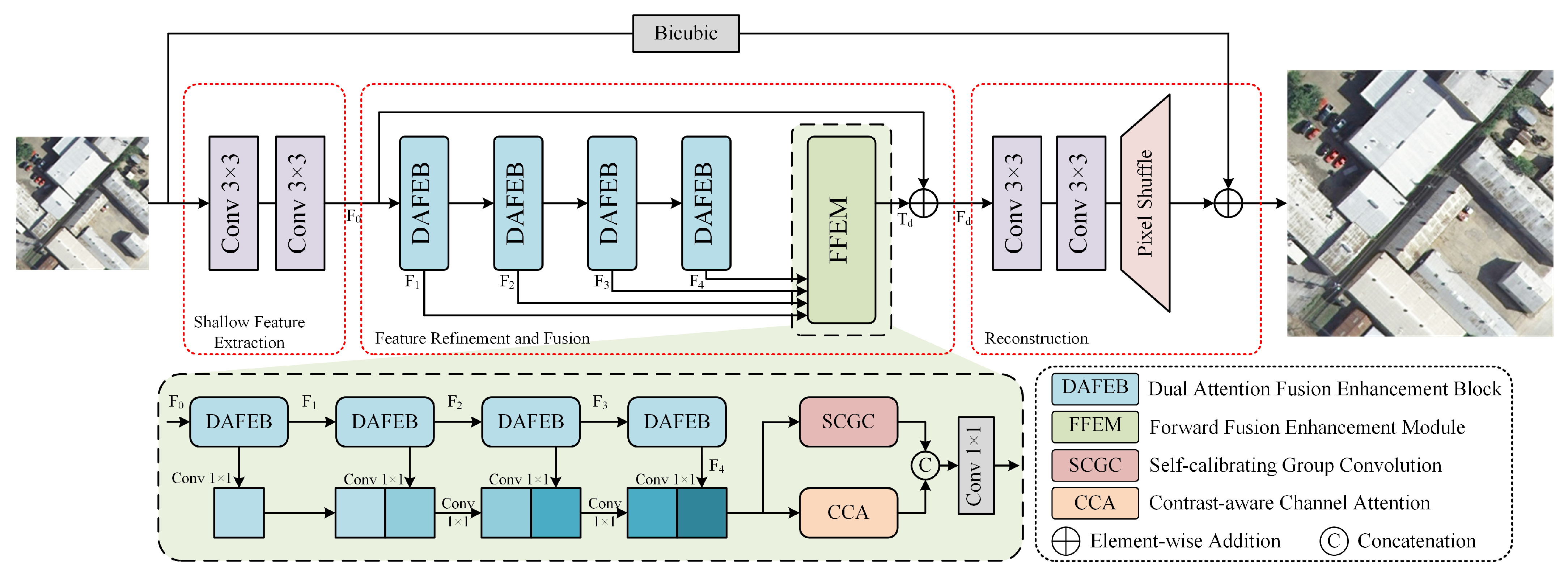
Figure 2.
Overview of the proposed Dual Attention Fusion Enhancement Network (DAFEN) architecture. The shallow feature extraction and reconstruction parts are utilized to extract coarse features and enlarge the features s times (e.g., ×2, ×3, ×4), respectively. The Feature Refinement and Fusion part with four DAFEBs carries the main feature expression ability. The FFEM can generate more contextual information via forward sequential concatenation.
Figure 3.
Structure of Dual Attention Fusion Enhancement Block (DAFEB).
Figure 3.
Structure of Dual Attention Fusion Enhancement Block (DAFEB).
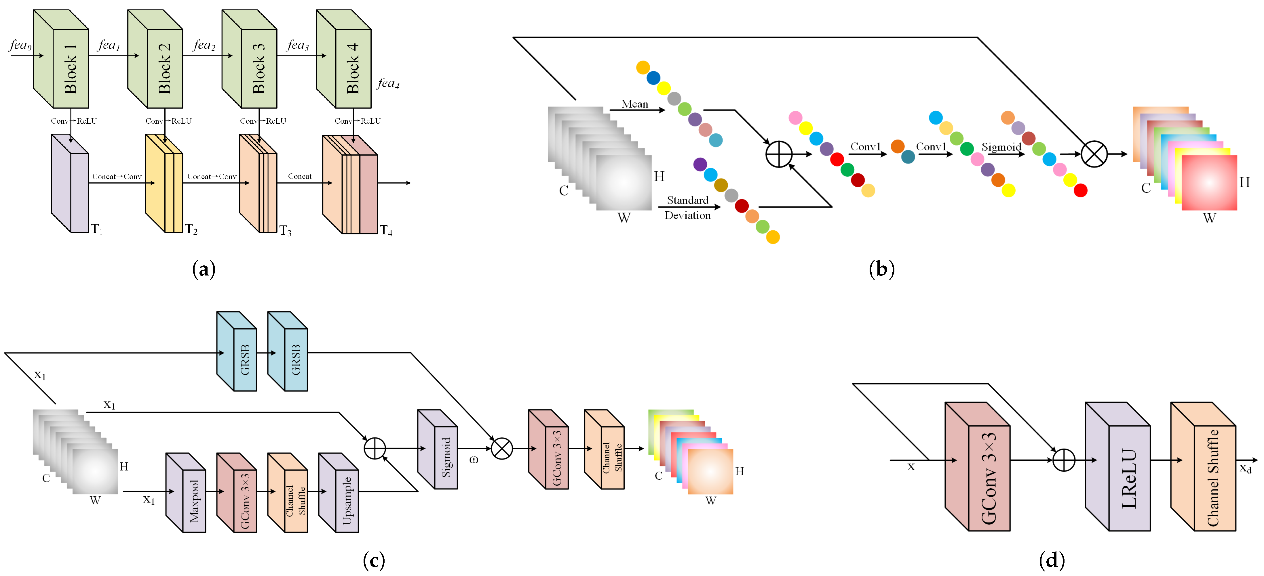
Figure 4.
Illustrations of the proposed Forward Fusion Enhancement Module (FFEM). (a) The forward fusion structure by using forward sequential concatenation is illustrated by taking four blocks as an example. (b) The Contrast-aware Channel Attention (CCA). (c) The Self-Calibrated Group Convolution (SCGC). (d) The Group Residual Shuffle Block (GRSB).
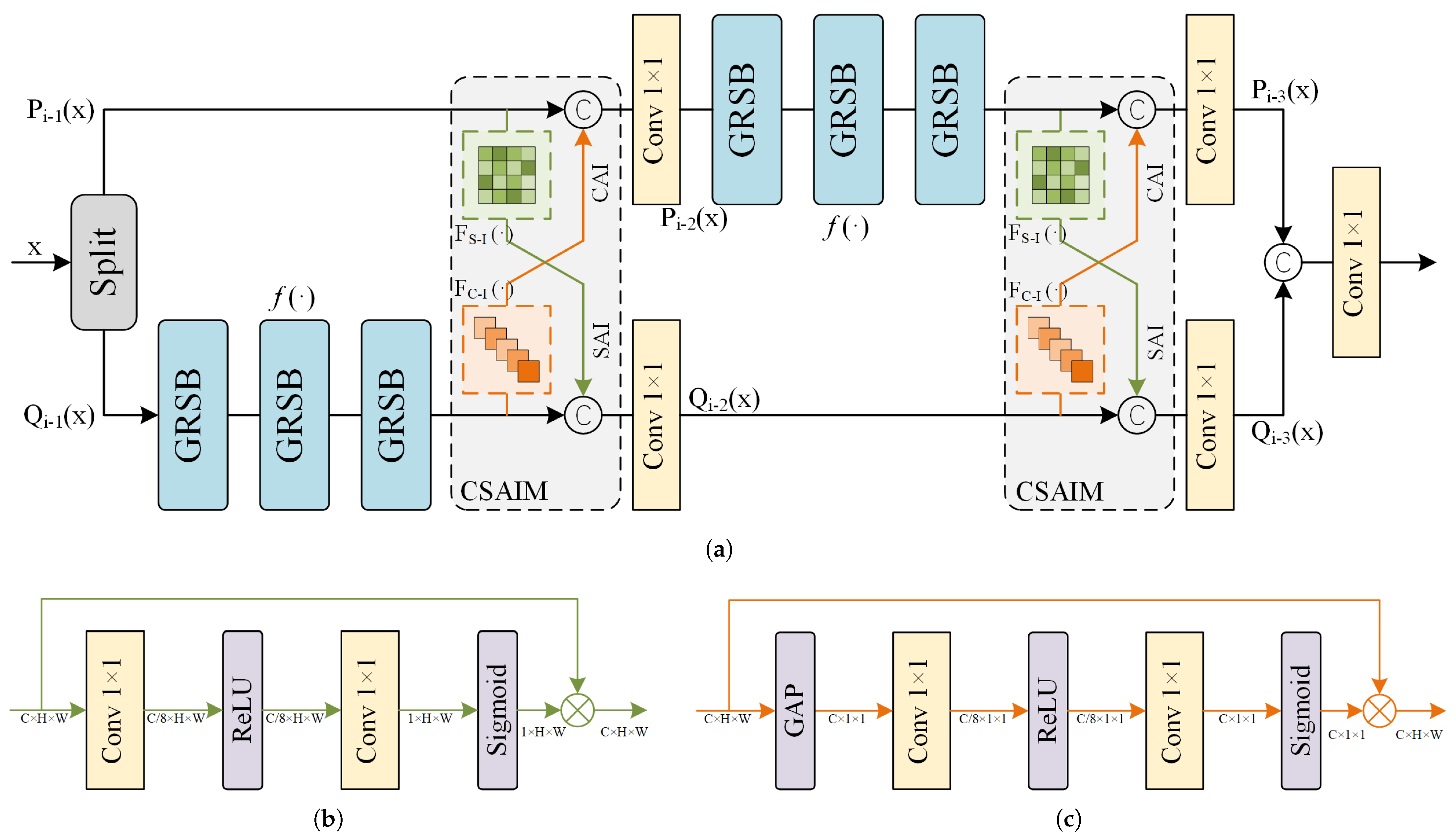
Figure 5.
(a) The Channel-Spatial Lattice Block (CSLB), where the Channel-Spatial Attention Interaction Module (CSAIM) includes the Spatial Attention Interaction (SAI) and the Channel Attention Interaction (CAI). ‘Split’ represents the channel separation operation. (b) The Spatial Attention Interaction (SAI). (c) The Channel Attention Interaction (CAI).
Figure 6.
Visualization results of several SR methods and our proposed networks (DAFEN and DAFEN-S) on UC-Merced for ×4 SR.
Figure 6.
Visualization results of several SR methods and our proposed networks (DAFEN and DAFEN-S) on UC-Merced for ×4 SR.
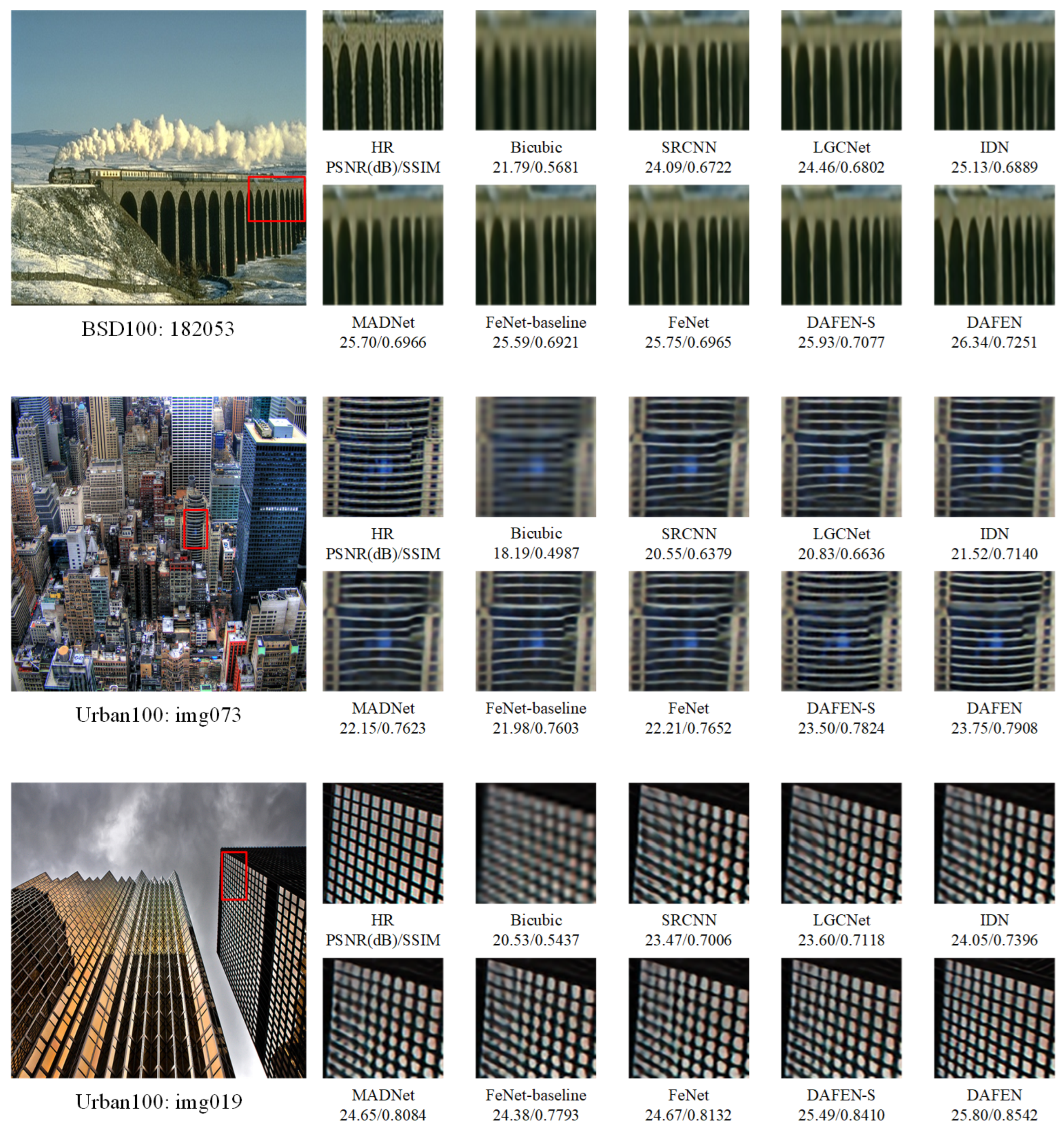
Figure 7.
Visualization results of several SR methods and our proposed networks (DAFEN and DAFEN-S) on BSD100 and Urban100 datasets for ×4 SR.
Figure 7.
Visualization results of several SR methods and our proposed networks (DAFEN and DAFEN-S) on BSD100 and Urban100 datasets for ×4 SR.
Figure 8.
Visualization results of our proposed networks (DAFEN and DAFEN-S) and other SR methods on real remote-sensing images for ×4 SR. (a) Residential areas and farmland. (b) Terraces and roads.
Figure 8.
Visualization results of our proposed networks (DAFEN and DAFEN-S) and other SR methods on real remote-sensing images for ×4 SR. (a) Residential areas and farmland. (b) Terraces and roads.
Figure 9.
Visualization results for the ablation experiments on the CSLB design.
Figure 9.
Visualization results for the ablation experiments on the CSLB design.
Figure 10.
Average feature maps from the ablation experiments on the FFEM design at different stages of the DAFEN.
Figure 10.
Average feature maps from the ablation experiments on the FFEM design at different stages of the DAFEN.
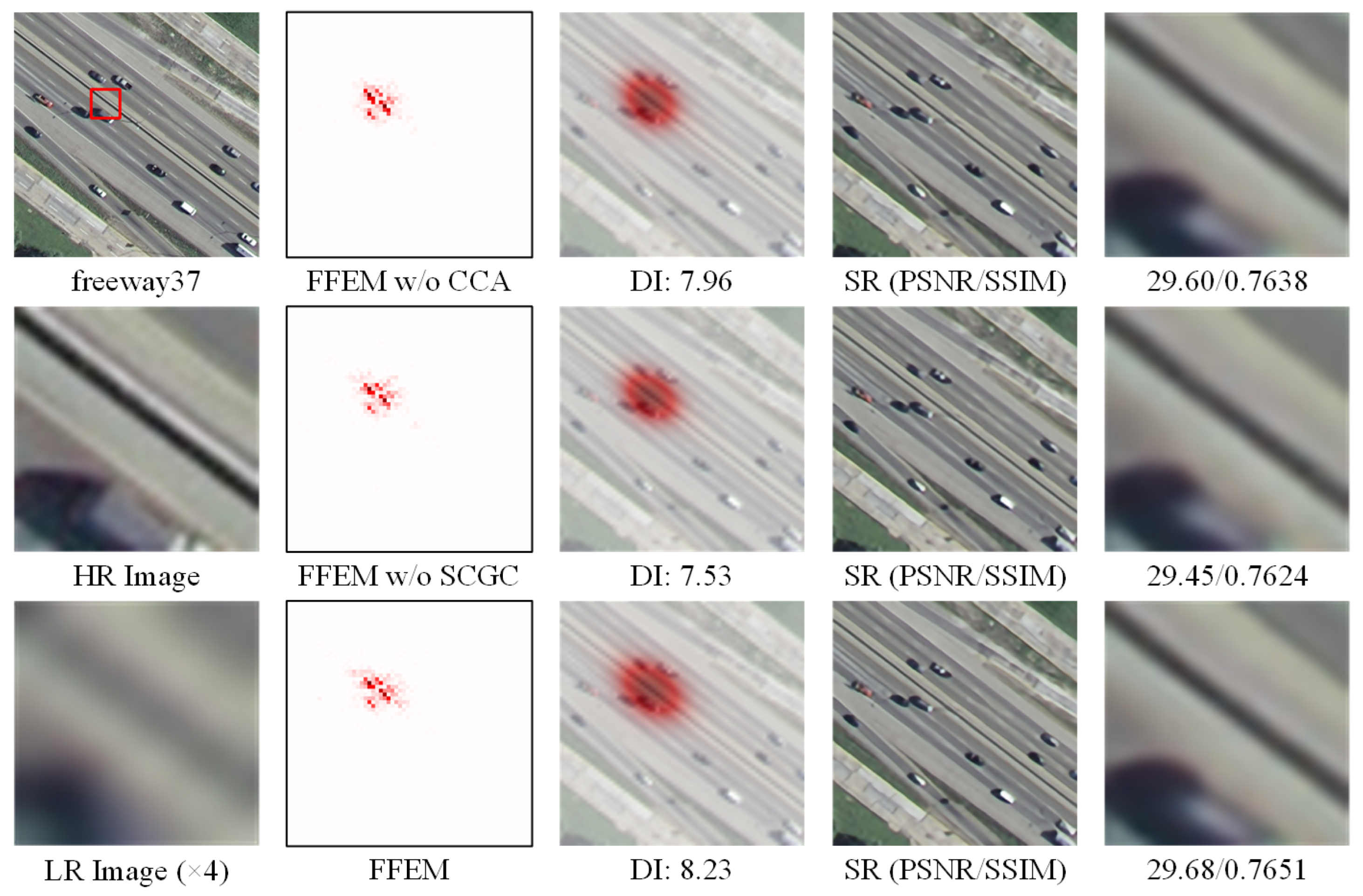
Figure 11.
LAM results for the ablation experiments on the FFEM design. LAM reflects the importance of each pixel in the input LR image during the reconstruction of the marked blocks. The red-marked points indicate the pixels that contribute to the reconstruction process. The Diffusion Index (DI) reflects the range of involved pixels, with a higher DI indicating a wider range of utilized pixels.
Figure 12.
Network average feature maps visualization.
Figure 12.
Network average feature maps visualization.
Table 1.
Implementation details and hyperparameter settings of our methods and comparative lightweight methods.
Table 1.
Implementation details and hyperparameter settings of our methods and comparative lightweight methods.
| Method | Optim_g | Betas | lr | Gamma | Loss Type | Batch Size | Patch Size | Use_hflip | Use_rot |
|---|
| LGCNet [21] | ADAM | [0.9,0.999] | | 0.1 | | 128 | 41 × 41 | false | false |
| IDN [51] | ADAM | [0.9,0.999] | | 0.1 | | 64 | 26 × 26 | true | true |
| LESRCNN [73] | ADAM | [0.9,0.999] | | 0.5 | | 64 | 64 × 64 | true | true |
| MADNet [74] | ADAM | [0.9,0.999] | | 0.5 | | 16 | 48 × 48 | true | true |
| CTN [48] | ADAM | [0.9,0.999] | | 0.5 | | 16 | 48 × 48 | true | true |
| FeNet-baseline [46] | ADAM | [0.9,0.999] | | 0.5 | | 16 | 192 × 192 | true | true |
| FeNet [46] | ADAM | [0.9,0.999] | | 0.5 | | 16 | 192 × 192 | true | true |
| FDENet [57] | ADAM | [0.9,0.999] | | 0.5 | | 16 | 192 × 192 | true | true |
| DARN-S [56] | ADAM | [0.9,0.999] | | 0.5 | | 64 | 64 × 64 | true | true |
| AMFFN [41] | ADAM | [0.9,0.999] | | 0.5 | | 16 | 48 × 48 | true | true |
| IFIN-S [55] | ADAM | [0.9,0.99] | | 0.5 | | 16 | 60 × 60 | true | true |
| BMFENet [58] | ADAM | [0.9,0.999] | | 0.5 | | 16 | 192 × 192 | true | true |
| TARN [49] | ADAM | [0.9,0.999] | | 0.5 | | 16 | 256 × 256 | true | true |
| DAFEN-S(ours) | ADAM | [0.9,0.999] | | 0.5 | | 16 | 192 × 192 | true | true |
| DAFEN(ours) | ADAM | [0.9,0.999] | | 0.5 | | 16 | 192 × 192 | true | true |
Table 2.
Impact of hyperparameter selection on model performance and complexity at a scaling factor of ×4 on the RS-T1 dataset. The Multi-Adds is calculated corresponding to a 1280 × 720 HR image.
Table 2.
Impact of hyperparameter selection on model performance and complexity at a scaling factor of ×4 on the RS-T1 dataset. The Multi-Adds is calculated corresponding to a 1280 × 720 HR image.
| Variant | Params | Multi-Adds | RS-T1(x4)
PSNR/SSIM |
|---|
| Loss type: | 431 K | 21.8 G | 29.73/0.7669 |
| batch size: 32 | 431 K | 21.8 G | 29.81/0.7694 |
| batch size: 8 | 431 K | 21.8 G | 29.80/0.7689 |
| patch size: 256 | 431 K | 38.8 G | 29.82/0.7695 |
| patch size: 128 | 431 K | 9.7 G | 29.80/0.7691 |
| Use_hflip: false | 431 K | 21.8 G | 29.76/0.7681 |
| Use_rot: false | 431 K | 21.8 G | 29.78/0.7685 |
| DAFEN | 431 K | 21.8 G | 29.82/0.7701 |
Table 3.
Quantitative evaluation results for SR on two RSI test datasets. PSNR and SSIM values are provided. ‘-’ denotes the results are not provided. The best and second-best results are highlighted in red and blue, respectively. The Multi-Adds is calculated corresponding to a 1280 × 720 HR image.
Table 3.
Quantitative evaluation results for SR on two RSI test datasets. PSNR and SSIM values are provided. ‘-’ denotes the results are not provided. The best and second-best results are highlighted in red and blue, respectively. The Multi-Adds is calculated corresponding to a 1280 × 720 HR image.
| Method | Scale | Params | Multi-Adds | RS-T1 PSNR/SSIM | RS-T2 PSNR/SSIM |
|---|
| Bicubic | ×2 | - | - | 33.25/0.8934 | 30.64/0.8837 |
| LGCNet [21] | ×2 | 193 K | 178.1 G | 35.65/0.9298 | 33.47/0.9281 |
| IDN [51] | ×2 | 553 K | 124.6 G | 36.13/0.9339 | 34.07/0.9329 |
| LESRCNN [73] | ×2 | 626 K | 281.5 G | 36.04/0.9328 | 34.00/0.9320 |
| CTN [48] | ×2 | 402 K | 60.9 G | 36.30/0.9243 | 34.31/0.9346 |
| FeNet-baseline [46] | ×2 | 158 K | 35.2 G | 36.10/0.9331 | 34.10/0.9326 |
| FeNet [46] | ×2 | 351 K | 77.9 G | 36.23/0.9341 | 34.22/0.9337 |
| FDENet [57] | ×2 | 480 K | 138.7 G | 36.26/0.9346 | 34.28/0.9338 |
| DARN-S [56] | ×2 | 350 K | 78.9 G | 36.31/0.9347 | 34.35/0.9348 |
| AMFFN [41] | ×2 | 298 K | 61.5 G | 36.39/0.9357 | 34.34/0.9346 |
| IFIN-S [55] | ×2 | 451 K | 110.6 G | 36.38/0.9356 | 34.42/0.9352 |
| BMFENet [58] | ×2 | 465 K | 115.0 G | 36.42/0.9362 | 34.43/0.9356 |
| DAFEN-S (ours) | ×2 | 188 K | 37.5 G | 36.28/0.9352 | 34.24/0.9338 |
| DAFEN (ours) | ×2 | 416 K | 83.6 G | 36.42/0.9365 | 34.39/0.9357 |
| Bicubic | ×3 | - | - | 29.73/0.7818 | 27.23/0.7697 |
| LGCNet [21] | ×3 | 193 K | 79.0 G | 31.30/0.8314 | 29.03/0.8312 |
| IDN [51] | ×3 | 553 K | 56.3 G | 31.73/0.8430 | 29.59/0.8450 |
| LESRCNN [73] | ×3 | 810 K | 238.9 G | 31.68/0.8398 | 29.65/0.8444 |
| CTN [48] | ×3 | 402 K | 37.1 G | 31.91/0.8454 | 29.83/0.8489 |
| FeNet-baseline [46] | ×3 | 163 K | 16.7 G | 31.73/0.8377 | 29.61/0.8446 |
| FeNet [46] | ×3 | 357 K | 35.2 G | 31.89/0.8432 | 29.80/0.8481 |
| FDENet [57] | ×3 | 488 K | 61.7 G | 31.98/0.8488 | 29.88/0.8489 |
| DARN-S [56] | ×3 | 355 K | 35.0 G | 32.00/0.8483 | 29.98/0.8518 |
| AMFFN [41] | ×3 | 305 K | 27.9 G | 31.94/0.8457 | 29.91/0.8504 |
| IFIN-S [55] | ×3 | 459 K | 51.0 G | 32.04/0.8448 | 30.03/0.8535 |
| BMFENet [58] | ×3 | 470 K | 51.7 G | 31.99/0.8465 | 29.97/0.8514 |
| DAFEN-S (ours) | ×3 | 192 K | 17.1 G | 31.93/0.8459 | 29.81/0.8485 |
| DAFEN (ours) | ×3 | 422 K | 37.7 G | 32.13/0.8527 | 29.98/0.8516 |
| Bicubic | ×4 | - | - | 27.91/0.6968 | 25.40/0.6770 |
| LGCNet [21] | ×4 | 193 K | 44.5 G | 29.13/0.7481 | 26.76/0.7426 |
| IDN [51] | ×4 | 553 K | 32.3 G | 29.56/0.7623 | 27.31/0.7627 |
| LESRCNN [73] | ×4 | 774 K | 241.6 G | 29.62/0.7625 | 27.41/0.7646 |
| CTN [48] | ×4 | 413 K | 25.6 G | 29.71/0.7666 | 27.52/0.7704 |
| FeNet-baseline [46] | ×4 | 169 K | 9.4 G | 29.57/0.7626 | 27.31/0.7619 |
| FeNet [46] | ×4 | 366 K | 20.4 G | 29.70/0.7688 | 27.45/0.7672 |
| FDENet [57] | ×4 | 501 K | 35.9 G | 29.72/0.7658 | 27.54/0.7697 |
| DARN-S [56] | ×4 | 363 K | 19.7 G | 29.78/0.7682 | 27.59/0.7732 |
| AMFFN [41] | ×4 | 314 K | 16.2 G | 29.76/0.7674 | 27.57/0.7701 |
| IFIN-S [55] | ×4 | 470 K | 31.6 G | 29.84/0.7724 | 27.68/0.7763 |
| BMFENet [58] | ×4 | 477 K | 29.4 G | 29.81/0.7700 | 27.62/0.7730 |
| DAFEN-S (ours) | ×4 | 198 K | 10.0 G | 29.70/0.7673 | 27.46/0.7677 |
| DAFEN (ours) | ×4 | 431K | 21.8 G | 29.82/0.7701 | 27.62/0.7737 |
Table 4.
Quantitative evaluation results for SR on four benchmark datasets. PSNR and SSIM values are provided. ‘-’ denotes the results are not provided. The best and second-best results are highlighted in red and blue, respectively. The Multi-Adds is calculated corresponding to a 1280 × 720 HR image.
| Method | Scale | Params | Multi-Adds | Set5 PSNR/SSIM | Set14 PSNR/SSIM | BSD100 PSNR/SSIM | Urban100 PSNR/SSIM |
|---|
| Bicubic | ×2 | - | - | 33.66/0.9299 | 30.24/0.8688 | 29.56/0.8431 | 26.88/0.8403 |
| LGCNet [21] | ×2 | 193 K | 178.1 G | 37.31/0.9580 | 32.94/0.9120 | 31.74/0.8939 | 30.53/0.9112 |
| IDN [51] | ×2 | 553 K | 124.6 G | 37.83/0.9600 | 33.30/0.9148 | 32.08/0.8985 | 31.27/0.9196 |
| MADNet [74] | ×2 | 878 K | 187.1 G | 37.85/0.9600 | 33.39/0.9161 | 32.05/0.8981 | 31.59/0.9234 |
| FeNet-baseline [46] | ×2 | 158 K | 35.2 G | 37.77/0.9597 | 33.28/0.9151 | 31.98/0.8973 | 31.46/0.9215 |
| FeNet [46] | ×2 | 351 K | 77.9 G | 37.90/0.9602 | 33.45/0.9162 | 32.09/0.8985 | 31.75/0.9245 |
| FDENet [57] | ×2 | 480 K | 138.7 G | 37.89/0.9594 | 33.50/0.9170 | 32.15/0.8988 | 32.02/0.9270 |
| DARN-S [56] | ×2 | 350 K | 78.9 G | 37.97/0.9609 | 33.54/0.9172 | 32.19/0.9005 | 32.14/0.9284 |
| IFIN-S [55] | ×2 | 451 K | 110.6 G | 38.00/0.9606 | 33.66/0.9181 | 32.18/0.8996 | 32.14/0.9284 |
| BMFENet [58] | ×2 | 465 K | 115.0 G | 38.04/0.9605 | 33.62/0.9180 | 32.22/0.9004 | 32.29/0.9300 |
| TARN [49] | ×2 | 687 K | - | 38.09/0.9608 | 33.65/0.9183 | 32.22/0.9003 | 32.20/0.9289 |
| DAFEN-S (ours) | ×2 | 188 K | 37.5 G | 37.94/0.9605 | 33.41/0.9159 | 32.12/0.8991 | 31.76/0.9248 |
| DAFEN (ours) | ×2 | 416 K | 83.6 G | 38.04/0.9617 | 33.55/0.9175 | 32.22/0.9010 | 32.20/0.9291 |
| Bicubic | ×3 | - | - | 30.39/0.8682 | 27.55/0.7742 | 27.21/0.7385 | 24.46/0.7349 |
| LGCNet [21] | ×3 | 193 K | 79.0 G | 33.32/0.9172 | 29.67/0.8289 | 28.63/0.7923 | 26.77/0.8180 |
| IDN [51] | ×3 | 553 K | 56.3 G | 34.11/0.9253 | 29.99/0.8354 | 28.95/0.8013 | 27.42/0.8359 |
| MADNet [74] | ×3 | 930 K | 88.4 G | 34.14/0.9251 | 30.20/0.8395 | 28.98/0.8023 | 27.78/0.8439 |
| FeNet-baseline [46] | ×3 | 163 K | 16.7 G | 33.99/0.9240 | 30.02/0.8359 | 28.90/0.8000 | 27.55/0.8391 |
| FeNet [46] | ×3 | 357 K | 35.2 G | 34.21/0.9256 | 30.15/0.8383 | 28.98/0.8020 | 27.82/0.8447 |
| FDENet [57] | ×3 | 488 K | 61.7 G | 34.28/0.9253 | 30.33/0.8415 | 29.05/0.8033 | 28.03/0.8494 |
| DARN-S [56] | ×3 | 355 K | 35.0 G | 34.35/0.9274 | 30.34/0.8428 | 29.09/0.8065 | 28.17/0.8528 |
| IFIN-S [55] | ×3 | 459 K | 51.0 G | 34.45/0.9278 | 30.47/0.8442 | 29.13/0.8064 | 28.32/0.8560 |
| BMFENet [58] | ×3 | 470 K | 51.7 G | 34.34/0.9271 | 30.27/0.8407 | 29.08/0.8049 | 28.18/0.8534 |
| TARN [49] | ×3 | 754 K | - | 34.42/0.9275 | 30.37/0.8430 | 29.12/0.8056 | 28.19/0.8529 |
| DAFEN-S (ours) | ×3 | 192 K | 17.1 G | 34.25/0.9261 | 30.18/0.8389 | 29.02/0.8031 | 27.76/0.8451 |
| DAFEN (ours) | ×3 | 422 K | 37.7 G | 34.43/0.9275 | 30.37/0.8434 | 29.12/0.8057 | 28.12/0.8517 |
| Bicubic | ×4 | - | - | 28.42/0.8104 | 26.00/0.7027 | 25.96/0.6675 | 23.14/0.6577 |
| LGCNet [21] | ×4 | 193 K | 44.5 G | 30.87/0.8746 | 27.82/0.7630 | 27.08/0.7186 | 24.82/0.7399 |
| IDN [51] | ×4 | 553 K | 32.3 G | 31.82/0.8903 | 28.25/0.7730 | 27.41/0.7297 | 25.41/0.7632 |
| MADNet [74] | ×4 | 1002 K | 54.1 G | 32.01/0.8925 | 28.45/0.7781 | 27.47/0.7327 | 25.77/0.7751 |
| FeNet-baseline [46] | ×4 | 169 K | 9.4 G | 31.80/0.8886 | 28.31/0.7742 | 27.38/0.7289 | 25.53/0.7670 |
| FeNet [46] | ×4 | 366 K | 20.4 G | 32.02/0.8919 | 28.38/0.7764 | 27.47/0.7319 | 25.75/0.7747 |
| FDENet [57] | ×4 | 501 K | 35.9 G | 32.12/0.8929 | 28.52/0.7795 | 27.53/0.7339 | 25.97/0.7811 |
| DARN-S [56] | ×4 | 363 K | 19.7 G | 32.16/0.8951 | 28.58/0.7817 | 27.57/0.7374 | 26.08/0.7859 |
| IFIN-S [55] | ×4 | 470 K | 31.6 G | 32.27/0.8958 | 28.68/0.7834 | 27.62/0.7381 | 26.17/0.7890 |
| BMFENet [58] | ×4 | 477 K | 29.4 G | 32.22/0.8951 | 28.61/0.7812 | 27.54/0.7335 | 26.04/0.7852 |
| TARN [49] | ×4 | 835 K | - | 32.23/0.8955 | 28.65/0.7829 | 27.61/0.7368 | 26.15/0.7874 |
| DAFEN-S (ours) | ×4 | 198 K | 10.0 G | 32.00/0.8919 | 28.39/0.7773 | 27.49/0.7326 | 25.72/0.7758 |
| DAFEN (ours) | ×4 | 431 K | 21.8 G | 32.23/0.8948 | 28.59/0.7815 | 27.57/0.7376 | 26.01/0.7832 |
Table 5.
Comparison results with non-lightweight state-of-the-art methods at a scaling factor of ×3. Due to the higher model complexity of non-lightweight methods, we present the data using larger magnitude units for ease of comparison. The best and second-best results are highlighted in red and blue, respectively. The Multi-Adds is calculated corresponding to a 1280 × 720 HR image.
| Method | Params | Multi-Adds | Times |
|---|
| RCAN [14] | 15.67 M | 1.492 T | 0.12 s |
| SwinIR [36] | 11.55 M | 2.883 T | 0.23 s |
| HAT [18] | 20.53 M | 3.871 T | 0.32 s |
| DAFEN-S | 0.192M | 0.017T | 0.012s |
| DAFEN | 0.422M | 0.038T | 0.017s |
Table 6.
Quantify how lightweight the model is on RS-T1 dataset with a scaling factor of ×3. The best and second-best results are highlighted in red and blue, respectively. The Multi-Adds is calculated corresponding to a 1280 × 720 HR image.
Table 6.
Quantify how lightweight the model is on RS-T1 dataset with a scaling factor of ×3. The best and second-best results are highlighted in red and blue, respectively. The Multi-Adds is calculated corresponding to a 1280 × 720 HR image.
| Method | Params | Multi-Adds | Times | RS-T1(x3) PSNR/SSIM |
|---|
| FeNet [46] | 357 K | 35.2 G | 19.46 ms | 31.89/0.8432 |
| DARN [56] | 596 K | 58.4 G | 18.87 ms | 32.08/0.8470 |
| IFIN-S [55] | 459 K | 51.0 G | 143.34 ms | 32.04/0.8448 |
| DAFEN-S | 192 K | 17.1 G | 11.65 ms | 31.93/0.8459 |
| DAFEN | 422 K | 37.7 G | 17.31 ms | 32.13/0.8527 |
Table 7.
Ablation experiments on the design of the DAFEN on RS-T1, RS-T2, BSD100, and Urban100 datasets for ×4 SR.
Table 7.
Ablation experiments on the design of the DAFEN on RS-T1, RS-T2, BSD100, and Urban100 datasets for ×4 SR.
| Variant | Params | Multi-Adds | RS-T1 PSNR/SSIM | RS-T2 PSNR/SSIM | BSD100 PSNR/SSIM | Urban100 PSNR/SSIM |
|---|
| DAFEN w/o DAFEB | 683 K | 38.7 G | 29.82/0.7689 | 27.63/0.7744 | 27.58/0.7380 | 26.03/0.7840 |
| DAFEN w/o CSLB | 744 K | 40.2 G | 29.83/0.7694 | 27.61/0.7742 | 27.58/0.7383 | 26.05/0.7851 |
| DAFEN w/o FFEM | 315 K | 16.5 G | 29.75/0.7663 | 27.54/0.7706 | 27.52/0.7353 | 25.92/0.7794 |
| DAFEN | 431 K | 21.8 G | 29.82/0.7701 | 27.62/0.7737 | 27.57/0.7376 | 26.01/0.7832 |
Table 8.
Ablation experiments on the design of the CSLB on RS-T1, RS-T2, BSD100, and Urban100 datasets for ×4 SR.
Table 8.
Ablation experiments on the design of the CSLB on RS-T1, RS-T2, BSD100, and Urban100 datasets for ×4 SR.
| Variant | Params | Multi-Adds | RS-T1 PSNR/SSIM | RS-T2 PSNR/SSIM | BSD100 PSNR/SSIM | Urban100 PSNR/SSIM |
|---|
| CSLB w/o GRSB | 867 K | 46.9 G | 29.85/0.7708 | 27.68/0.7753 | 27.61/0.7386 | 26.13/0.7854 |
| CSLB w/o CSAIM | 434 K | 21.7 G | 29.80/0.7696 | 27.61/0.7735 | 27.54/0.7371 | 25.99/0.7831 |
| CSLB | 431 K | 21.8 G | 29.82/0.7701 | 27.62/0.7737 | 27.57/0.7376 | 26.01/0.7832 |
Table 9.
Ablation experiments on the design of the FFEM on RS-T1, RS-T2, BSD100, and Urban100 datasets for ×4 SR.
Table 9.
Ablation experiments on the design of the FFEM on RS-T1, RS-T2, BSD100, and Urban100 datasets for ×4 SR.
| Variant | Params | Multi-Adds | RS-T1 PSNR/SSIM | RS-T2 PSNR/SSIM | BSD100 PSNR/SSIM | Urban100 PSNR/SSIM |
|---|
| W/ 1x1Conv | 443K | 22.4G | 29.81/0.7695 | 27.59/0.7722 | 27.54/0.7367 | 26.00/0.7828 |
| W/ BFM | 431K | 21.8G | 29.79/0.7689 | 27.61/0.7735 | 27.56/0.7373 | 26.01/0.7831 |
| FFEM w/o SCGC | 303K | 15.8G | 29.73/0.7671 | 27.53/0.7705 | 27.49/0.7350 | 25.80/0.7765 |
| FFEM w/o CCA | 406K | 20.4G | 29.79/0.7688 | 27.60/0.7732 | 27.54/0.7365 | 25.95/0.7814 |
| FFEM | 431K | 21.8G | 29.82/0.7701 | 27.62/0.7737 | 27.57/0.7376 | 26.01/0.7832 |
Table 10.
Ablation experiments on the design of the lightweight convolution in DAFEN on RS-T1, RS-T2, BSD100, and Urban100 datasets for ×4 SR.
Table 10.
Ablation experiments on the design of the lightweight convolution in DAFEN on RS-T1, RS-T2, BSD100, and Urban100 datasets for ×4 SR.
| Variant | Params | Multi-Adds | RS-T1 PSNR/SSIM | RS-T2 PSNR/SSIM | BSD100 PSNR/SSIM | Urban100 PSNR/SSIM |
|---|
| W/ PSConv | 368 K | 18.7 G | 29.73/0.7665 | 27.54/0.7706 | 27.48/0.7346 | 25.89/0.7792 |
| W/ BSConv | 343 K | 17.5 G | 29.62/0.7634 | 27.42/0.7663 | 27.44/0.7317 | 25.80/0.7768 |
| W/ DSConv | 343 K | 17.5 G | 29.65/0.7642 | 27.40/0.7648 | 27.45/0.7324 | 25.81/0.7766 |
| DAFEN | 431 K | 21.8 G | 29.82/0.7701 | 27.62/0.7737 | 27.57/0.7376 | 26.01/0.7832 |
Table 11.
Ablation experiments on the design of the number of groups in group convolution on RS-T1, RS-T2, BSD100, and Urban100 datasets for ×4 SR.
Table 11.
Ablation experiments on the design of the number of groups in group convolution on RS-T1, RS-T2, BSD100, and Urban100 datasets for ×4 SR.
| Variant | Params | Multi-Adds | RS-T1 PSNR/SSIM | RS-T2 PSNR/SSIM | BSD100 PSNR/SSIM | Urban100 PSNR/SSIM |
|---|
| G = 2 | 628 K | 31.8 G | 29.84/0.7705 | 27.66/0.7746 | 27.59/0.7385 | 26.08/0.7844 |
| G = 4 | 431 K | 21.8 G | 29.82/0.7701 | 27.62/0.7737 | 27.57/0.7376 | 26.01/0.7832 |
| G = 8 | 333 K | 16.8 G | 29.77/0.7672 | 27.59/0.7727 | 27.54/0.7365 | 25.94/0.7808 |
Table 12.
Ablation experiments on the design of the number of DAFEBs and CSLBs on RS-T1, RS-T2, BSD100, and Urban100 datasets for ×4 SR.
Table 12.
Ablation experiments on the design of the number of DAFEBs and CSLBs on RS-T1, RS-T2, BSD100, and Urban100 datasets for ×4 SR.
| Variant | Params | Multi-Adds | RS-T1 PSNR/SSIM | RS-T2 PSNR/SSIM | BSD100 PSNR/SSIM | Urban100 PSNR/SSIM |
|---|
| = 4, = 1 | 289 K | 13.9 G | 29.76/0.7681 | 27.57/0.7716 | 27.53/0.7361 | 25.86/0.7787 |
| = 4, = 3 | 431 K | 21.8 G | 29.82/0.7701 | 27.62/0.7737 | 27.57/0.7376 | 26.01/0.7832 |
| = 4, = 5 | 574 K | 29.7 G | 29.86/0.7694 | 27.71/0.7759 | 27.59/0.7383 | 26.11/0.7861 |
| = 3, = 3 | 345 K | 17.5 G | 29.79/0.7676 | 27.60/0.7730 | 27.54/0.7362 | 25.92/0.7798 |
| = 5, = 3 | 517 K | 26.0 G | 29.84/0.7700 | 27.65/0.7746 | 27.59/0.7380 | 26.05/0.7849 |
| = 6, = 3 | 603 K | 30.3 G | 29.86/0.7704 | 27.70/0.7764 | 27.61/0.7386 | 26.12/0.7863 |


