
U-Shaped Dual Attention Vision Mamba Network for Satellite Remote Sensing Single-Image Dehazing

 ,
,  , ,
, ,
Abstract
1. Introduction
2. Related Work
2.1. Image Dehazing Algorithms
2.2. State Space Models
3. Proposed Method
3.1. SSMs and Mamba Model
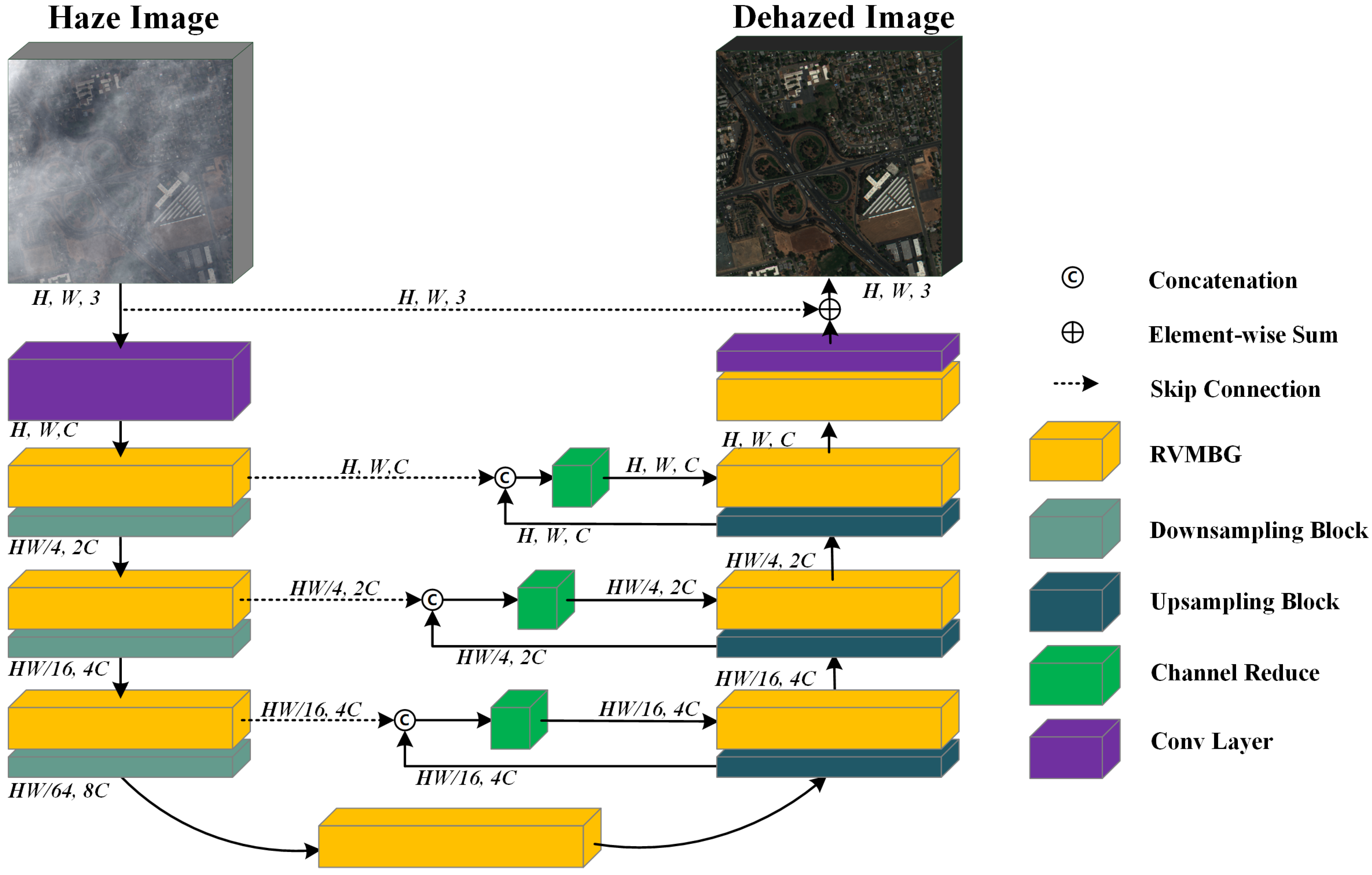
3.2. Overview of Proposed UDAVM-Net Architecture
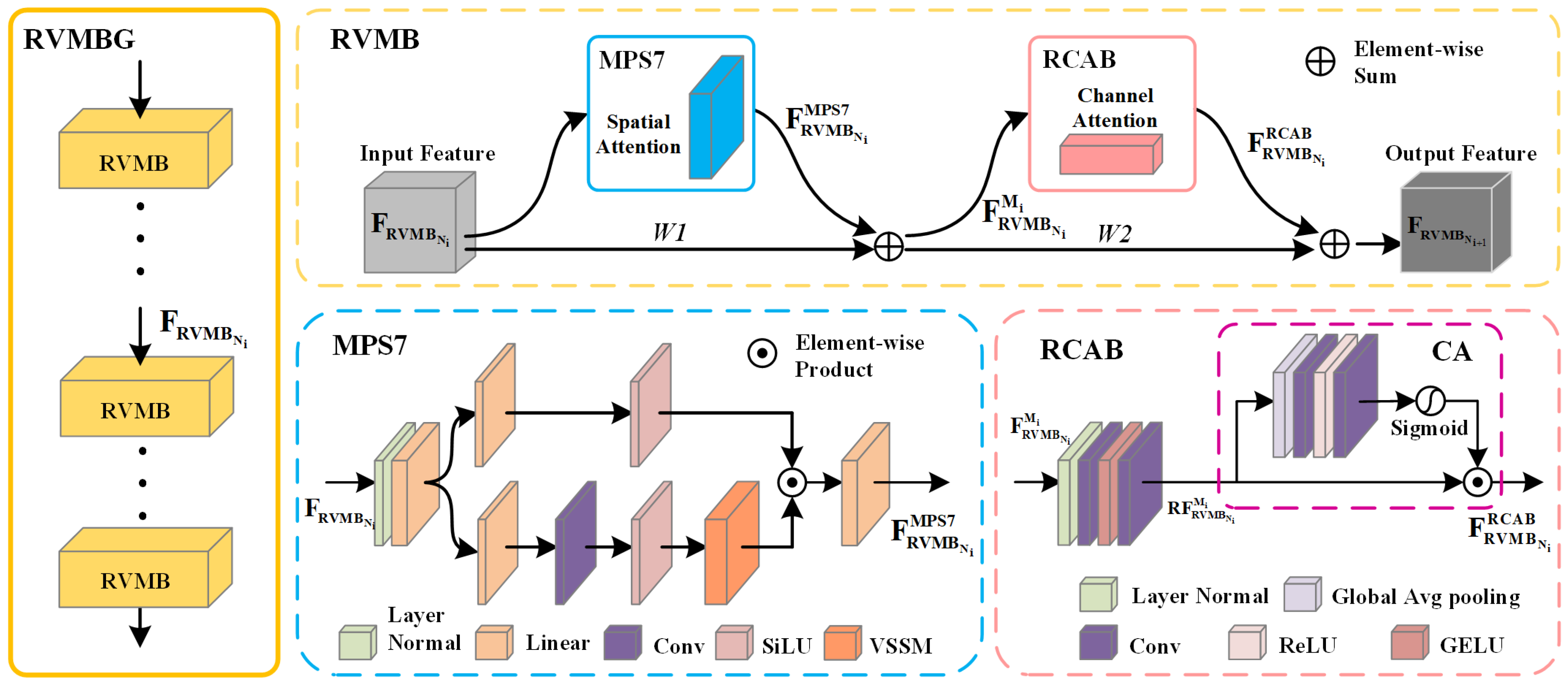
3.3. Residual Visual Mamba Block
3.4. MPS7 Block
3.5. RCAB Block
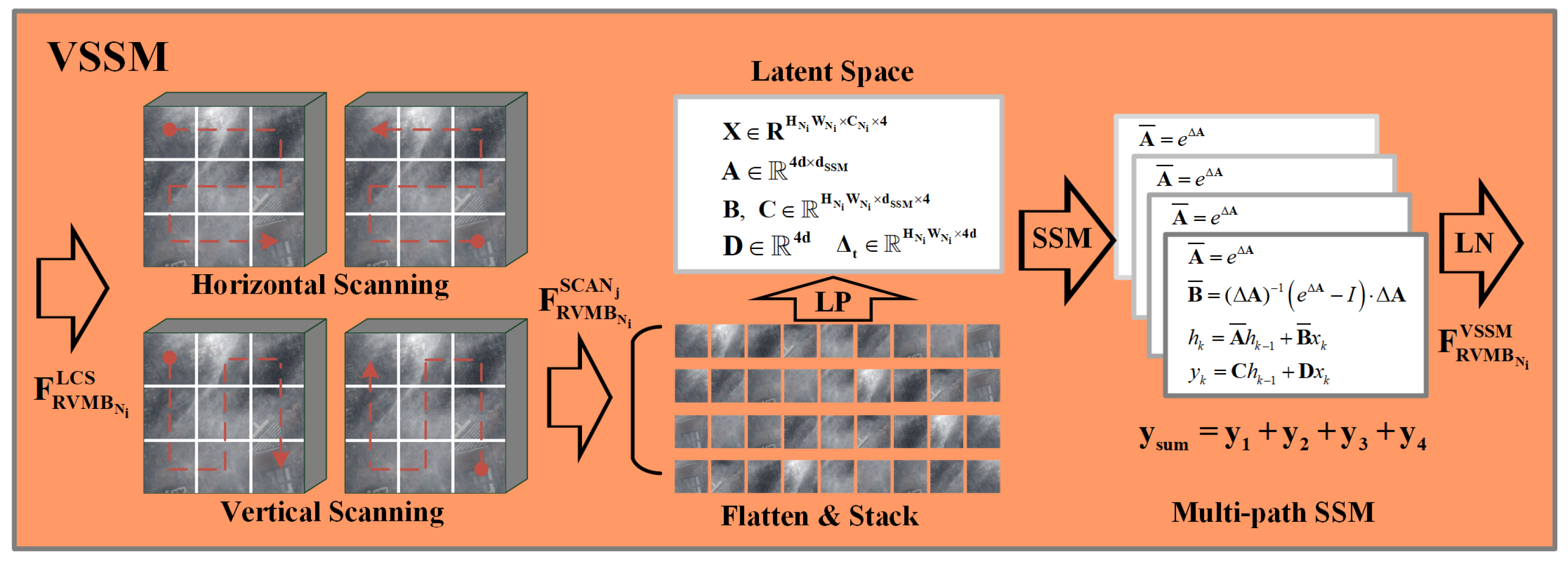
3.6. VSSM Block
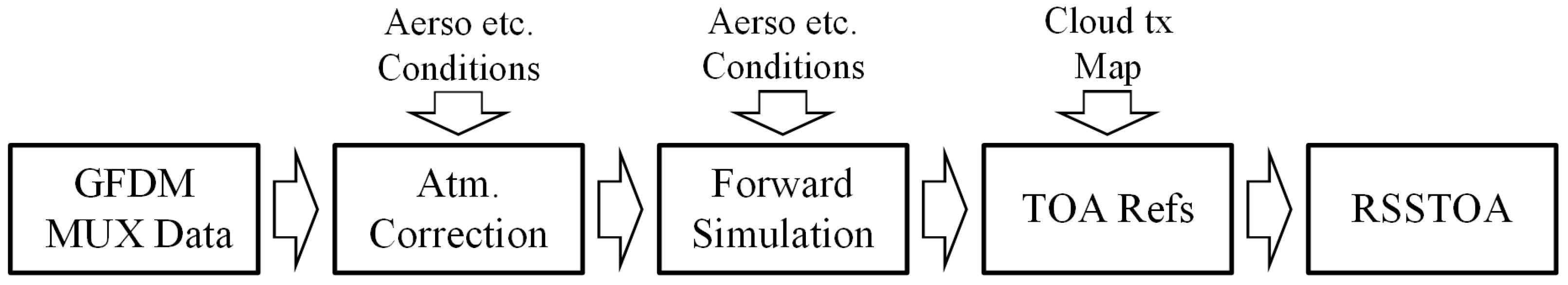
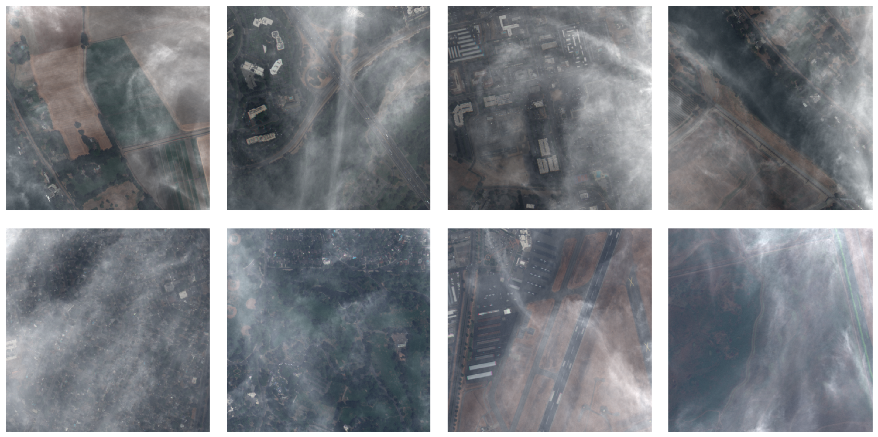
4. RSSTOA Dataset
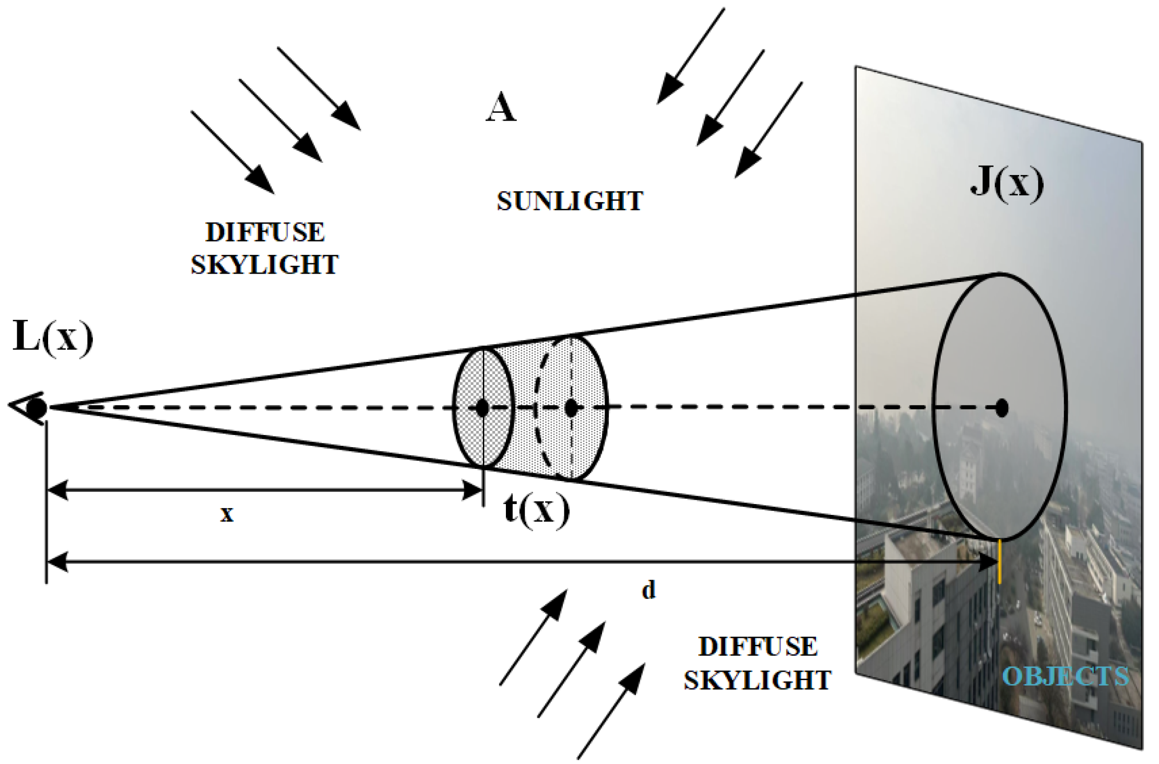
4.1. Synthetic Model for Dehazing Based on Radiative Transfer Theory
4.1.1. TOA Apparent Reflectance Without Cloud
4.1.2. TOA Reflectance Contaminated by Cloud
4.1.3. Pipeline for Generating Cloud Transmission Maps
4.2. Synthesis Pipeline
5. Experimental Results
5.1. Experimental Settings
5.1.1. Dataset
5.1.2. Parameter Settings
5.1.3. Evaluation Metric and Benchmark Methods
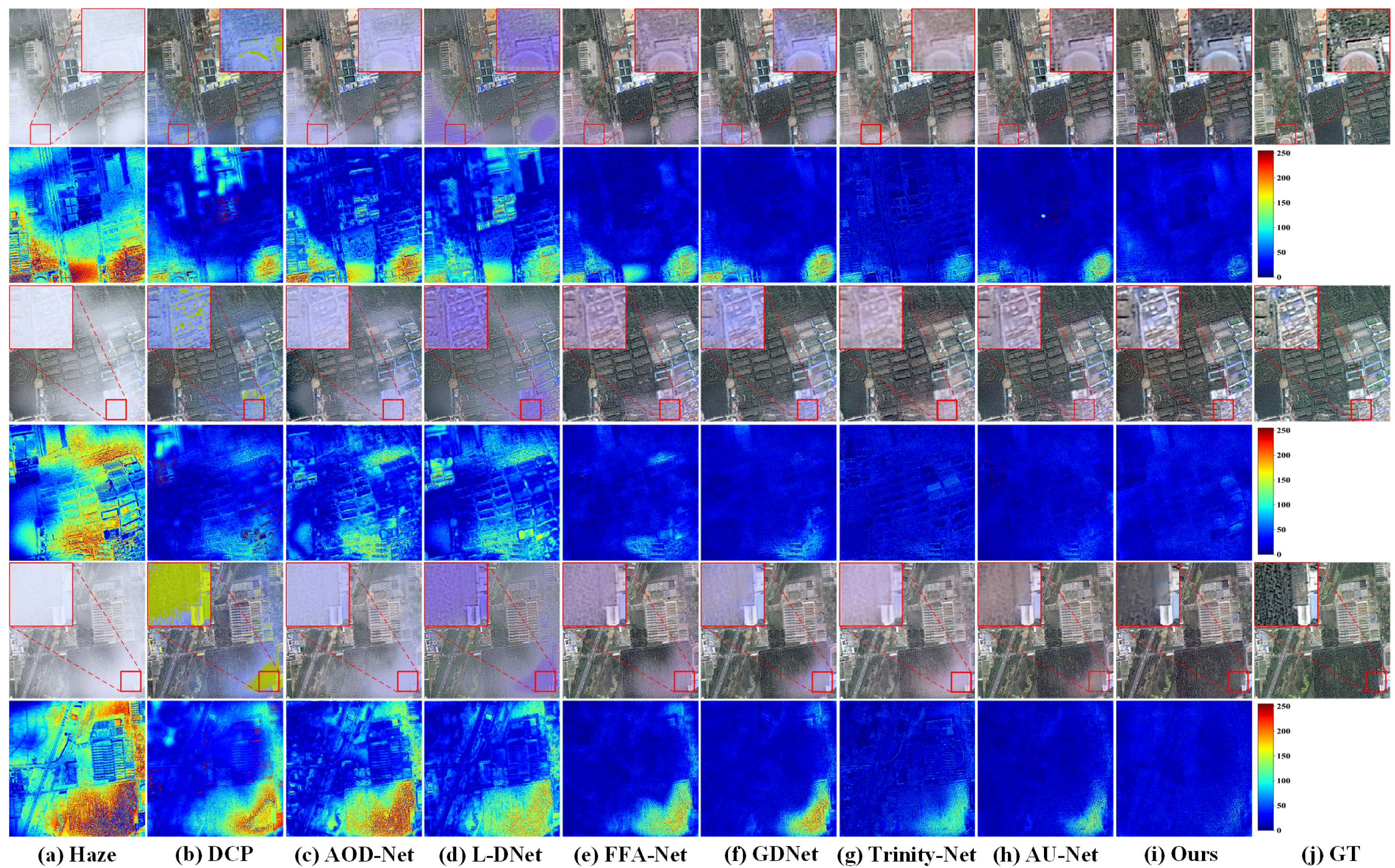
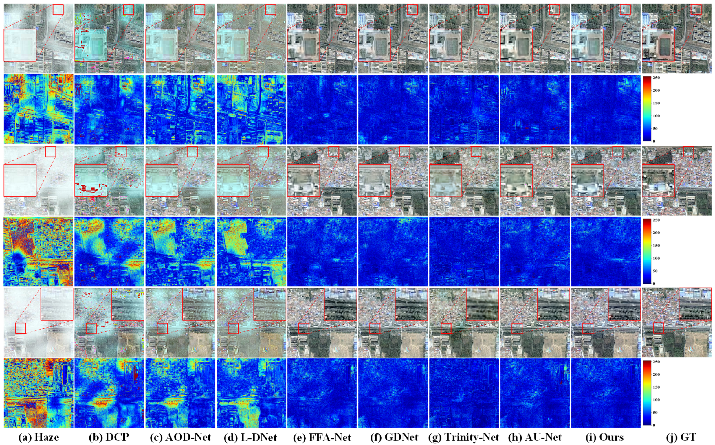
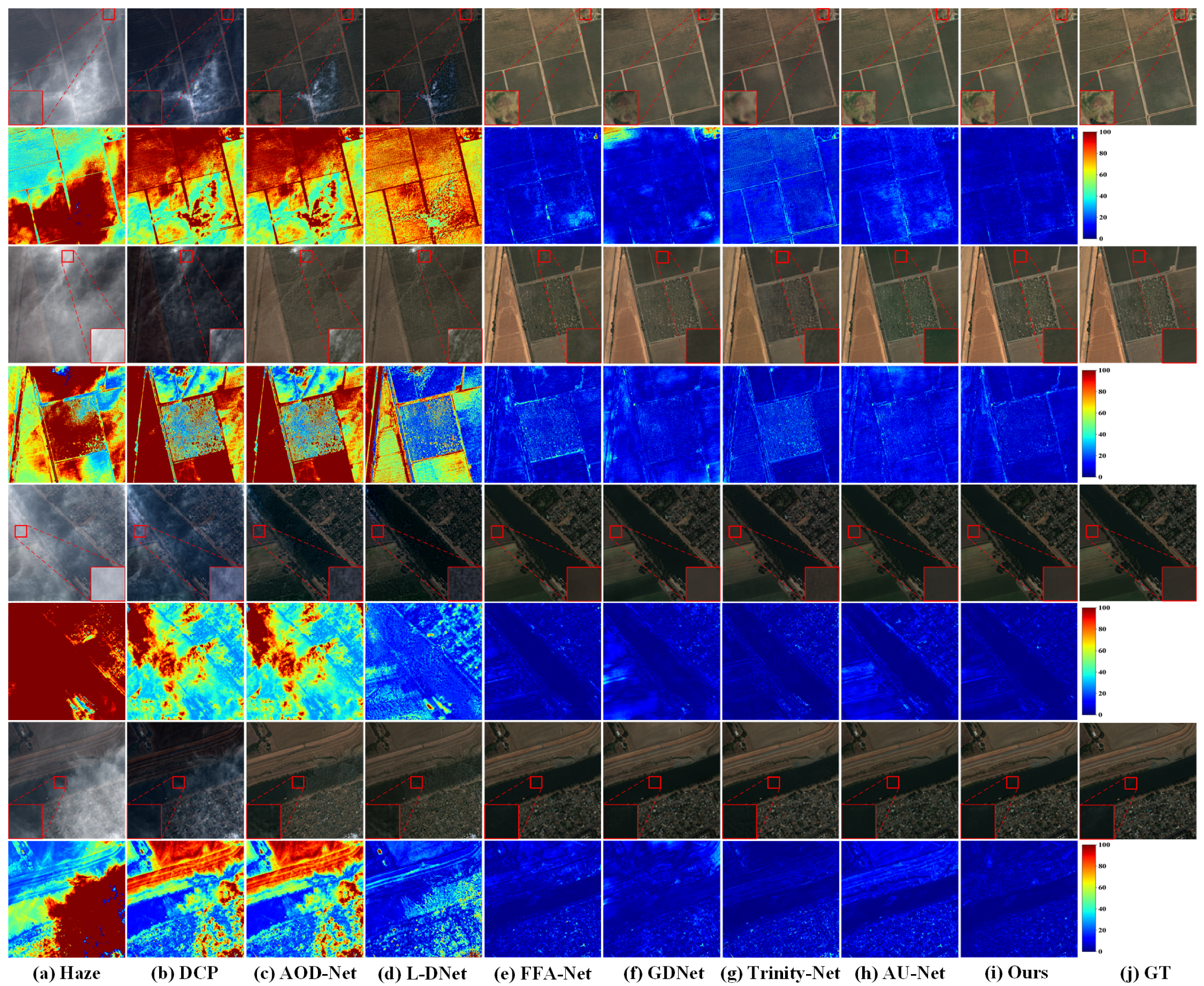
5.2. Qualitative Comparisons
5.3. Quantitative Comparison
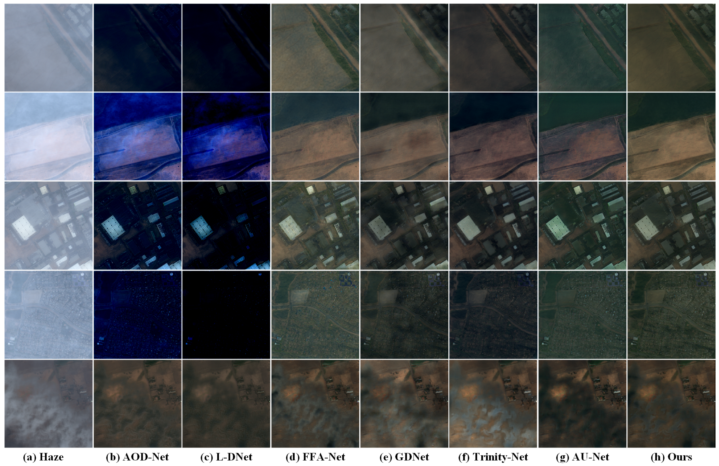
5.4. Results and Analysis on Real Remote Sensing Data
6. Discussion
6.1. Ablation Study
- (1)
- Base: UDAVM-Net without the VSSM module in MSP7 and without the CA module in RCAB.
- (2)
- Base + CA: The base framework with CA in RCAB.
- (3)
- Base + VSSM_SHS + CA: The base framework with VSSM using single-horizontal-scanning (SHS), and with CA in RCAB.
- (4)
- Base + VSSM_HVS + CA: The base framework with VSSM using horizontal-vertical-scanning (HVS), and with CA in RCAB.
- (5)
- Base + VSSM + CA: The base framework with both VSSM in MSP7 and CA in RCAB, corresponding to the proposed UDAVM-Net.
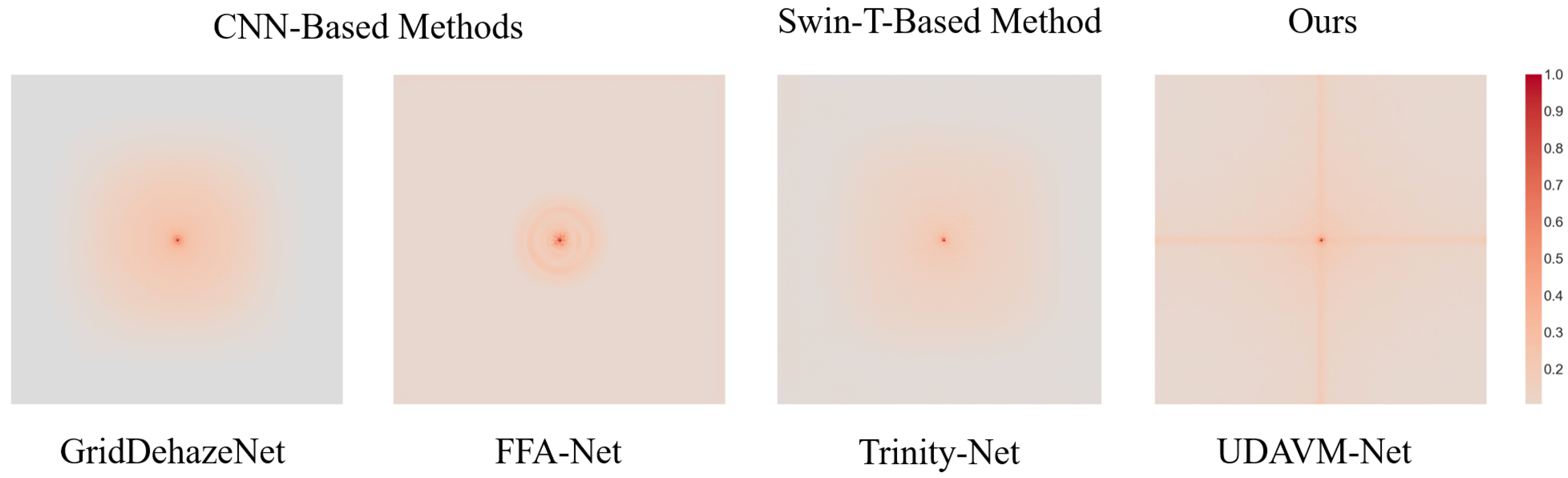
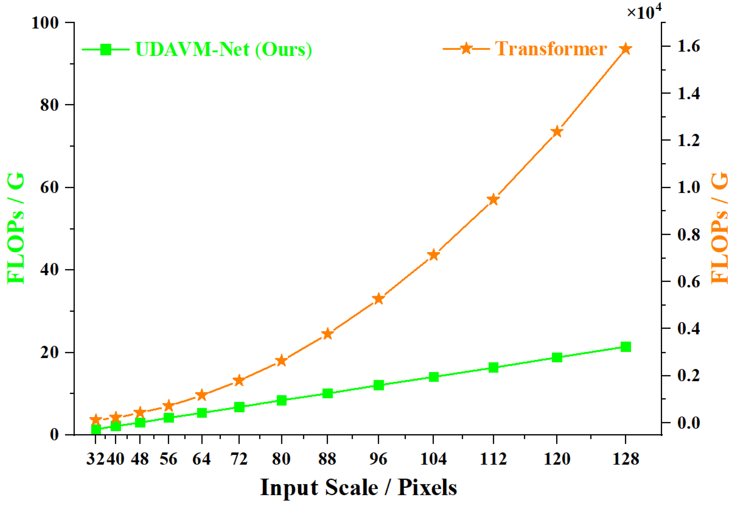
6.2. Model Complexity
7. Conclusions
Author Contributions
Funding
Data Availability Statement
Conflicts of Interest
References
- Cai, B.; Xu, X.; Jia, K.; Qing, C.; Tao, D. DehazeNet: An End-to-End System for Single Image Haze Removal. IEEE Trans. Image Process. 2016, 25, 5187–5198. [Google Scholar] [CrossRef] [PubMed]
- Li, B.; Peng, X.; Wang, Z.; Xu, J.; Feng, D. AOD-Net: All-in-One Dehazing Network. In Proceedings of the 2017 IEEE International Conference on Computer Vision (ICCV), Venice, Italy, 22–29 October 2017; pp. 4780–4788. [Google Scholar] [CrossRef]
- Jiang, H.; Lu, N. Multi-Scale Residual Convolutional Neural Network for Haze Removal of Remote Sensing Images. Remote Sens. 2018, 10, 945. [Google Scholar] [CrossRef]
- Gu, Z.; Zhan, Z.; Yuan, Q.; Yan, L. Single Remote Sensing Image Dehazing Using a Prior-Based Dense Attentive Network. Remote Sens. 2019, 11, 3008. [Google Scholar] [CrossRef]
- Liu, X.; Ma, Y.; Shi, Z.; Chen, J. GridDehazeNet: Attention-Based Multi-Scale Network for Image Dehazing. In Proceedings of the 2019 IEEE/CVF International Conference on Computer Vision (ICCV), Seoul, Republic of Korea, 27 October–2 November 2019; pp. 7313–7322. [Google Scholar] [CrossRef]
- Qin, X.; Wang, Z.; Bai, Y.; Xie, X.; Jia, H. FFA-Net: Feature Fusion Attention Network for Single Image Dehazing. In Proceedings of the AAAI Conference on Artificial Intelligence, New York, NY, USA, 7–12 February 2020; Volume 34, pp. 11908–11915. [Google Scholar] [CrossRef]
- Li, Y.; Chen, X. A Coarse-to-Fine Two-Stage Attentive Network for Haze Removal of Remote Sensing Images. IEEE Geosci. Remote. Sens. Lett. 2021, 18, 1751–1755. [Google Scholar] [CrossRef]
- Ullah, H.; Muhammad, K.; Irfan, M.; Anwar, S.; Sajjad, M.; Imran, A.S.; de Albuquerque, V.H. Light-DehazeNet: A Novel Lightweight CNN Architecture for Single Image Dehazing. IEEE Trans. Image Process. 2021, 30, 8968–8982. [Google Scholar] [CrossRef] [PubMed]
- Jiang, B.; Chen, G.; Wang, J.; Ma, H.; Wang, L.; Wang, Y.; Chen, X. Deep Dehazing Network for Remote Sensing Image with Non-Uniform Haze. Remote Sens. 2021, 13, 4443. [Google Scholar] [CrossRef]
- Guo, J.; Yang, J.; Yue, H.; Tan, H.; Hou, C.; Li, K. RSDehazeNet: Dehazing Network With Channel Refinement for Multispectral Remote Sensing Images. IEEE Trans. Geosci. Remote. Sens. 2021, 59, 2535–2549. [Google Scholar] [CrossRef]
- Wei, J.; Wu, Y.; Chen, L.; Yang, K.; Lian, R. Zero-Shot Remote Sensing Image Dehazing Based on a Re-Degradation Haze Imaging Model. Remote Sens. 2022, 14, 5737. [Google Scholar] [CrossRef]
- Li, J.; Chen, M.; Hou, S.; Wang, Y.; Luo, Q.; Wang, C. An Improved S2A-Net Algorithm for Ship Object Detection in Optical Remote Sensing Images. Remote Sens. 2023, 15, 4559. [Google Scholar] [CrossRef]
- Sun, H.; Luo, Z.; Ren, D.; Hu, W.; Du, B.; Yang, W.; Wan, J.; Zhang, L. Partial Siamese With Multiscale Bi-Codec Networks for Remote Sensing Image Haze Removal. IEEE Trans. Geosci. Remote. Sens. 2023, 61, 4106516. [Google Scholar] [CrossRef]
- Wei, J.; Cao, Y.; Yang, K.; Chen, L.; Wu, Y. Self-Supervised Remote Sensing Image Dehazing Network Based on Zero-Shot Learning. Remote Sens. 2023, 15, 2732. [Google Scholar] [CrossRef]
- Dong, W.; Wang, C.; Sun, H.; Teng, Y.; Liu, H.; Zhang, Y.; Zhang, K.; Li, X.; Xu, X. End-to-End Detail-Enhanced Dehazing Network for Remote Sensing Images. Remote Sens. 2024, 16, 225. [Google Scholar] [CrossRef]
- Fang, J.; Wang, X.; Li, Y.; Zhang, X.; Zhang, B.; Gade, M. GLUENet: An Efficient Network for Remote Sensing Image Dehazing with Gated Linear Units and Efficient Channel Attention. Remote Sens. 2024, 16, 1450. [Google Scholar] [CrossRef]
- He, Y.; Li, C.; Li, X.; Bai, T. A Lightweight CNN Based on Axial Depthwise Convolution and Hybrid Attention for Remote Sensing Image Dehazing. Remote Sens. 2024, 16, 2822. [Google Scholar] [CrossRef]
- Zhou, H.; Wang, L.; Li, Q.; Guan, X.; Tao, T. Multi-Dimensional and Multi-Scale Physical Dehazing Network for Remote Sensing Images. Remote Sens. 2024, 16, 4780. [Google Scholar] [CrossRef]
- Du, Y.; Li, J.; Sheng, Q.; Zhu, Y.; Wang, B.; Ling, X. Dehazing Network: Asymmetric Unet Based on Physical Model. IEEE Trans. Geosci. Remote Sens. 2024, 62, 5607412. [Google Scholar] [CrossRef]
- Chi, K.; Yuan, Y.; Wang, Q. Trinity-Net: Gradient-Guided Swin Transformer-Based Remote Sensing Image Dehazing and Beyond. IEEE Trans. Geosci. Remote Sens. 2023, 61, 4702914. [Google Scholar] [CrossRef]
- Song, Y.; He, Z.; Qian, H.; Du, X. Vision Transformers for Single Image Dehazing. IEEE Trans. Image Process. 2023, 32, 1927–1941. [Google Scholar] [CrossRef]
- Zhang, X.; Xie, F.; Ding, H.; Yan, S.; Shi, Z. Proxy and Cross-Stripes Integration Transformer for Remote Sensing Image Dehazing. IEEE Trans. Geosci. Remote Sens. 2024, 62, 5640315. [Google Scholar] [CrossRef]
- Nie, J.; Xie, J.; Sun, H. Remote Sensing Image Dehazing via a Local Context-Enriched Transformer. Remote Sens. 2024, 16, 1422. [Google Scholar] [CrossRef]
- Yang, L.; Cao, J.; Wang, H.; Dong, S.; Ning, H. Hierarchical Semantic-Guided Contextual Structure-Aware Network for Spectral Satellite Image Dehazing. Remote Sens. 2024, 16, 1525. [Google Scholar] [CrossRef]
- Wang, Y.; Zhao, J.; Yao, L.; Fu, C. Depth-Guided Dehazing Network for Long-Range Aerial Scenes. Remote Sens. 2024, 16, 2081. [Google Scholar] [CrossRef]
- Narasimhan, S.G.; Nayar, S.K. Removing weather effects from monochrome images. In Proceedings of the 2001 IEEE Computer Society Conference on Computer Vision and Pattern Recognition (CVPR 2001), Kauai, HI, USA, 8–14 December 2001; p. 2. [Google Scholar] [CrossRef]
- Wang, J.; Lu, K.; Xue, J.; He, N.; Shao, L. Single Image Dehazing Based on the Physical Model and MSRCR Algorithm. IEEE Trans. Circuits Syst. Video Technol. 2018, 28, 2190–2199. [Google Scholar] [CrossRef]
- Zhu, R.; Wang, L.J. Improved wavelet transform algorithm for single image dehazing. Optik 2014, 125, 3064–3066. [Google Scholar] [CrossRef]
- He, K.; Sun, J.; Tang, X. Single Image Haze Removal Using Dark Channel Prior. Trans. Pattern Anal. Mach. Intell. 2011, 33, 2341–2353. [Google Scholar] [CrossRef]
- Fang, S.; Xia, X.; Huo, X.; Chen, C. Image Dehazing Using Polarization Effects of Objects and Airlight. Opt. Express 2014, 22, 19523–19537. [Google Scholar] [CrossRef]
- Wang, R.; Wang, G. Single Image Recovery in Scattering Medium by Propagating Deconvolution. Opt. Express 2014, 22, 8114–8119. [Google Scholar] [CrossRef]
- Zhu, Q.; Mai, J.; Shao, L. A Fast Single Image Haze Removal Algorithm Using Color Attenuation Prior. IEEE Trans. Image Process. 2015, 24, 3522–3533. [Google Scholar] [CrossRef]
- Shi, X.; Huang, F.; Ju, L.; Fan, Z.; Zhao, S.; Chen, S. Hierarchical Deconvolution Dehazing Method Based on Transmission Map Segmentation. Opt. Express 2023, 31, 43234–43249. [Google Scholar] [CrossRef]
- Wang, T.; Du, L.; Yi, W.; Hong, J.; Zhang, L.; Zheng, J.; Li, C.; Ma, X.; Zhang, D.; Fang, W.; et al. An adaptive atmospheric correction algorithm for the effective adjacency effect correction of submeter-scale spatial resolution optical satellite images: Application to a WorldView-3 panchromatic image. Remote Sens. Environ. 2021, 259, 112412. [Google Scholar] [CrossRef]
- Luo, W.; Li, Y.; Urtasun, R.; Zemel, R. Understanding the Effective Receptive Field in Deep Convolutional Neural Networks. arXiv 2017, arXiv:1701.04128. [Google Scholar]
- Ding, X.; Zhang, X.; Zhou, Y.; Han, J.; Ding, G.; Sun, J. Scaling Up Your Kernels to 31 × 31: Revisiting Large Kernel Design in CNNs. arXiv 2022, arXiv:2203.06717. [Google Scholar]
- Dosovitskiy, A.; Beyer, L.; Kolesnikov, A.; Weissenborn, D.; Zhai, X.; Unterthiner, T.; Dehghani, M.; Minderer, M.; Heigold, G.; Gelly, S.; et al. An Image is Worth 16 × 16 Words: Transformers for Image Recognition at Scale. arXiv 2021, arXiv:2010.11929. [Google Scholar]
- Vaswani, A.; Shazeer, N.; Parmar, N.; Uszkoreit, J.; Jones, L.; Gomez, A.N.; Kaiser, Ł.; Polosukhin, I. Attention is All You Need. In Advances in Neural Information Processing Systems, Proceedings of the Annual Conference on Neural Information Processing Systems 2017, Long Beach, CA, USA, 4–9 December 2017; Guyon, I., Von Luxburg, U., Bengio, S., Wallach, H., Fergus, R., Vishwanathan, S., Garnett, R., Eds.; Curran Associates, Inc.: Red Hook, NY, USA, 2017; Volume 30, Available online: https://proceedings.neurips.cc/paper_files/paper/2017/file/3f5ee243547dee91fbd053c1c4a845aa-Paper.pdf (accessed on 4 December 2017).
- Liu, Z.; Lin, Y.; Cao, Y.; Hu, H.; Wei, Y.; Zhang, Z.; Lin, S.; Guo, B. Swin Transformer: Hierarchical Vision Transformer using Shifted Windows. In Proceedings of the 2021 IEEE/CVF International Conference on Computer Vision (ICCV), Montreal, QC, Canada, 10–17 October 2021; pp. 9992–10002. Available online: http://doi.ieeecomputersociety.org/10.1109/ICCV48922.2021.00986 (accessed on 28 February 2022).
- Gu, A.; Dao, T.; Ermon, S.; Rudra, A.; Ré, C. HiPPO: Recurrent Memory with Optimal Polynomial Projections. In Advances in Neural Information Processing Systems, Proceedings of the Annual Conference on Neural Information Processing Systems 2020, Online, 6–12 December 2020; Larochelle, H., Ranzato, M., Hadsell, R., Balcan, M.F., Lin, H., Eds.; Curran Associates, Inc.: Red Hook, NY, USA, 2020; pp. 1474–1487. Available online: https://proceedings.neurips.cc/paper_files/paper/2020/file/102f0bb6efb3a6128a3c750dd16729be-Paper.pdf (accessed on 6 December 2020).
- Gu, A.; Johnson, I.; Goel, K.; Saab, K.; Dao, T.; Rudra, A.; Ré, C. Combining Recurrent, Convolutional, and Continuous-time Models with Linear State Space Layers. In Advances in Neural Information Processing Systems, Proceedings of the 35th Conference on Neural Information Processing Systems (NeurIPS 2021), Online, 6–14 December 2021; Ranzato, M., Beygelzimer, A., Dauphin, Y., Liang, P.S., Vaughan, J.W., Eds.; Curran Associates, Inc.: Red Hook, NY, USA, 2021; pp. 572–585. Available online: https://proceedings.neurips.cc/paper_files/paper/2021/file/05546b0e38ab9175cd905eebcc6ebb76-Paper.pdf (accessed on 6 December 2021).
- Gu, A.; Dao, T. Mamba: Linear-Time Sequence Modeling with Selective State Spaces. arXiv 2024, arXiv:2312.00752. [Google Scholar]
- Kalman, R.E. A new approach to linear filtering and prediction problems. ASME J. Basic Eng. 1960, 82, 35–45. [Google Scholar] [CrossRef]
- Chen, Z.; Brown, E.N. State space model. Scholarpedia 2013, 8, 30868. Available online: http://www.scholarpedia.org/article/State_space_model (accessed on 1 March 2024). [CrossRef]
- Liu, Y.; Tian, Y.; Zhao, Y.; Yu, H.; Xie, L.; Wang, Y.; Ye, Q.; Jiao, J.; Liu, Y. VMamba: Visual State Space Model. In Proceedings of the Thirty-Eighth Annual Conference on Neural Information Processing Systems, Vancouver, BC, Canada, 10–15 December 2024; Available online: https://openreview.net/forum?id=ZgtLQQR1K7 (accessed on 26 September 2024).
- Guo, H.; Li, J.; Dai, T.; Ouyang, Z.; Ren, X.; Xia, S.-T. MambaIR: A Simple Baseline for Image Restoration with State-Space Model. In Computer Vision—ECCV 2024, Proceedings of the 18th European Conference, Milan, Italy, 29 September–4 October 2024; Aleš, L., Ricci, E., Roth, S., Russakovsky, O., Sattler, T., Varol, G., Eds.; Springer Nature Switzerland: Cham, Switzerland, 2025; pp. 222–241. [Google Scholar] [CrossRef]
- Zheng, Z.; Wu, C. U-shaped Vision Mamba for Single Image Dehazing. arXiv 2024, arXiv:2402.04139. [Google Scholar]
- Ma, J.; Li, F.; Wang, B. U-Mamba: Enhancing Long-range Dependency for Biomedical Image Segmentation. arXiv 2024, arXiv:2401.04722. [Google Scholar]
- Ångström, A. The Parameters of Atmospheric Turbidity. Tellus 1964, 16, 64–75. [Google Scholar] [CrossRef]
- Vermote, E.F.; Tanre, D.; Deuze, J.L.; Herman, M.; Morcette, J.-J. Second Simulation of the Satellite Signal in the Solar Spectrum, 6S: An Overview. IEEE Trans. Geosci. Remote Sens. 1997, 35, 675–686. [Google Scholar] [CrossRef]
- Mitchell, O.R.; Delp, E.J.; Chen, P.L. Filtering to Remove Cloud Cover in Satellite Imagery. IEEE Trans. Geosci. Electron. 1977, 15, 137–141. [Google Scholar] [CrossRef]
- Li, J.; Wu, Z.; Hu, Z.; Zhang, J.; Li, M.; Mo, L.; Molinier, M. Thin Cloud Removal in Optical Remote Sensing Images Based on Generative Adversarial Networks and Physical Model of Cloud Distortion. ISPRS J. Photogramm. Remote Sens. 2020, 166, 373–389. [Google Scholar] [CrossRef]
- He, K.; Zhang, X.; Ren, S.; Sun, J. Deep Residual Learning for Image Recognition. In Proceedings of the IEEE Conference on Computer Vision and Pattern Recognition (CVPR), Las Vegas, NV, USA, 27–30 June 2016; pp. 770–778. [Google Scholar] [CrossRef]
- Wang, Z.; Zheng, J.-Q.; Zhang, Y.; Cui, G.; Li, L. Mamba-UNet: UNet-Like Pure Visual Mamba for Medical Image Segmentation. arXiv 2024, arXiv:2402.05079. [Google Scholar]
- Fu, D.Y.; Dao, T.; Saab, K.K.; Thomas, A.W.; Rudra, A.; Ré, C. Hungry Hungry Hippos: Towards Language Modeling with State Space Models. arXiv 2023, arXiv:2212.14052. [Google Scholar]
- Zhang, Y.; Li, K.; Li, K.; Wang, L.; Zhong, B.; Fu, Y. Image Super-Resolution Using Very Deep Residual Channel Attention Networks. In Proceedings of the European Conference on Computer Vision (ECCV), Munich, Germany, 8–14 September 2018. [Google Scholar]
- Ancuti, C.O.; Ancuti, C.; Timofte, R. NH-HAZE: An Image Dehazing Benchmark with Non-Homogeneous Hazy and Haze-Free Images. In Proceedings of the 2020 IEEE/CVF Conference on Computer Vision and Pattern Recognition Workshops (CVPRW), Seattle, WA, USA, 14–19 June 2020; pp. 1798–1805. [Google Scholar] [CrossRef]
- Ancuti, C.; Ancuti, C.O.; Timofte, R.; De Vleeschouwer, C. I-HAZE: A Dehazing Benchmark with Real Hazy and Haze-Free Indoor Images. In Advanced Concepts for Intelligent Vision Systems, Proceedings of the 19th International Conference, ACIVS 2018, Poitiers, France, 24–27 September 2018; Springer International Publishing: Cham, Switzerland, 2018; pp. 620–631. [Google Scholar] [CrossRef]
- Ancuti, C.O.; Ancuti, C.; Timofte, R.; De Vleeschouwer, C. O-HAZE: A Dehazing Benchmark with Real Hazy and Haze-Free Outdoor Images. In Proceedings of the 2018 IEEE/CVF Conference on Computer Vision and Pattern Recognition Workshops (CVPRW), Salt Lake City, UT, USA, 18–22 June 2018; pp. 867–8678. [Google Scholar] [CrossRef]
- Ancuti, C.O.; Ancuti, C.; Sbert, M.; Timofte, R. Dense-Haze: A Benchmark for Image Dehazing with Dense-Haze and Haze-Free Images. In Proceedings of the 2019 IEEE International Conference on Image Processing (ICIP), Taipei, Taiwan, 22–25 September 2019; pp. 1014–1018. [Google Scholar] [CrossRef]
- Ancuti, C.; Ancuti, C.O.; De Vleeschouwer, C. D-HAZY: A Dataset to Evaluate Quantitatively Dehazing Algorithms. In Proceedings of the 2016 IEEE International Conference on Image Processing (ICIP), Phoenix, AZ, USA, 25–28 September 2016; pp. 2226–2230. [Google Scholar] [CrossRef]
- Li, B.; Ren, W.; Fu, D.; Tao, D.; Feng, D.; Zeng, W.; Wang, Z. Benchmarking Single-Image Dehazing and Beyond. IEEE Trans. Image Process. 2019, 28, 492–505. [Google Scholar] [CrossRef]
- Qin, M.; Xie, F.; Li, W.; Shi, Z.; Zhang, H. Dehazing for Multispectral Remote Sensing Images Based on a Convolutional Neural Network With the Residual Architecture. IEEE J. Sel. Top. Appl. Earth Obs. Remote Sens. 2018, 11, 1645–1655. [Google Scholar] [CrossRef]
- Li, Z.; Hou, W.; Qiu, Z.; Ge, B.; Xie, Y.; Hong, J.; Ma, Y.; Peng, Z.; Fang, W.; Zhang, D.; et al. Preliminary On-Orbit Performance Test of the First Polarimetric Synchronization Monitoring Atmospheric Corrector (SMAC) On-Board High-Spatial Resolution Satellite Gao Fen Duo Mo (GFDM). IEEE Trans. Geosci. Remote Sens. 2022, 60, 4104014. [Google Scholar] [CrossRef]
- Hadjimitsis, D.G.; Clayton, C.R.I.; Retalis, A. On the Darkest Pixel Atmospheric Correction Algorithm: A Revised Procedure Applied Over Satellite Remotely Sensed Images Intended for Environmental Applications. In Remote Sensing for Environmental Monitoring, GIS Applications, and Geology III, Proceedings of the Remote Sensing, Barcelona, Spain, 8–12 September 2003; SPIE: Bellingham, WA, USA, 2004; Volume 5239, pp. 464–471. [Google Scholar] [CrossRef]
- Huang, B.; Li, Z.; Yang, C.; Sun, F.; Song, Y. Single Satellite Optical Imagery Dehazing using SAR Image Prior Based on Conditional Generative Adversarial Networks. In Proceedings of the 2020 IEEE Winter Conference on Applications of Computer Vision (WACV), Snowmass, CO, USA, 1–5 March 2020; pp. 1795–1802. [Google Scholar] [CrossRef]
- Kingma, D.P.; Ba, J. Adam: A Method for Stochastic Optimization. arXiv 2017, arXiv:1412.6980. [Google Scholar]
- Loshchilov, I.; Hutter, F. SGDR: Stochastic Gradient Descent with Warm Restarts. arXiv 2017, arXiv:1608.03983. [Google Scholar]
- Zhang, L.; Zhang, L.; Bovik, A.C. A Feature-Enriched Completely Blind Image Quality Evaluator. IEEE Trans. Image Process. 2015, 24, 2579–2591. [Google Scholar] [CrossRef]


| Methods | Thin Haze | Moderate Haze | Thick Haze | Average | |||||
|---|---|---|---|---|---|---|---|---|---|
| PSNR | SSIM | PSNR | SSIM | PSNR | SSIM | PSNR | SSIM | ||
| Classical | DCP [29] | 16.84 | 0.8215 | 19.04 | 0.8948 | 14.32 | 0.6931 | 16.73 | 0.8031 |
| CNN Based | AOD-Net [2] | 18.90 | 0.8521 | 18.50 | 0.8640 | 16.43 | 0.7505 | 17.94 | 0.8222 |
| Light-DehazeNet [8] | 18.20 | 0.8523 | 18.99 | 0.8876 | 15.49 | 0.7381 | 17.56 | 0.8260 | |
| FFA-Net [6] | 23.86 | 0.9183 | 24.57 | 0.9344 | 21.38 | 0.8506 | 23.27 | 0.9011 | |
| GridDehazeNet [5] | 25.18 | 0.9208 | 26.02 | 0.9390 | 21.81 | 0.8477 | 24.34 | 0.9025 | |
| AU-Net [19] | 22.72 | 0.9062 | 26.47 | 0.9410 | 21.25 | 0.8318 | 23.48 | 0.8930 | |
| Swin-T based | Trinity-Net [20] | 22.77 | 0.9367 | 24.78 | 0.9400 | 20.31 | 0.8895 | 22.62 | 0.9221 |
| Ours | UDAVM-Net | 26.79 | 0.9340 | 27.53 | 0.9521 | 23.48 | 0.8732 | 25.59 | 0.9198 |
| Methods | PSNR | SSIM | |
|---|---|---|---|
| Classical | DCP [29] | 19.89 | 0.7429 |
| CNN Based | AOD-Net [2] | 21.48 | 0.7843 |
| Light-DehazeNet [8] | 22.64 | 0.8006 | |
| FFA-Net [6] | 34.95 | 0.9619 | |
| GridDehazeNet [5] | 35.04 | 0.9681 | |
| AU-Net [19] | 32.36 | 0.9353 | |
| Swin-T based | Trinity-Net [20] | 33.25 | 0.9356 |
| Ours | UDAVM-Net | 38.03 | 0.9734 |
| Methods | Hazed Images | AOD- Net [2] | Light- DehazeNet [8] | FFA- Net [6] | Grid- DehazeNet [5] | Trinity- Net [20] | AU- Net [19] | UDAVM- Net |
|---|---|---|---|---|---|---|---|---|
| IL-NIQE | 58.94 | 64.80 | 73.92 | 44.62 | 49.22 | 45.43 | 44.45 | 43.82 |
| Model | PSNR | SSIM |
|---|---|---|
| Base | 24.32 | 0.9207 |
| Base + CA | 24.65 | 0.9217 |
| Base + VSSM_SHS + CA | 25.29 | 0.9260 |
| Base + VSSM_HVS + CA | 25.56 | 0.9249 |
| Base + VSSM + CA | 25.60 | 0.9273 |
| Methods | #Params | FLOPs | |
|---|---|---|---|
| Classical | DCP [29] | - | - |
| CNN based | AOD-Net [2] | 0.02 M | 0.03 G |
| Light-DehazeNet [8] | 0.03 M | 0.49 G | |
| FFA-Net [6] | 4.68 M | 75.54 G | |
| GridDehazeNet [5] | 0.96 M | 5.36 G | |
| AU-Net [19] | 7.14 M | 13.01 G | |
| Transformer based | Transformer [38] | 65 M | ≈ 15.88 T |
| ViT-B/16 [37] | 86 M | ≈ 11.2 G | |
| Swin-B [39] | 88 M | ≈ 5.03 G | |
| Trinity-Net [20] | 20.14 M | 7.61 G | |
| Ours | UDAVM-Net | 19.57 M | 21.34 G |
Disclaimer/Publisher’s Note: The statements, opinions and data contained in all publications are solely those of the individual author(s) and contributor(s) and not of MDPI and/or the editor(s). MDPI and/or the editor(s) disclaim responsibility for any injury to people or property resulting from any ideas, methods, instructions or products referred to in the content. |
© 2025 by the authors. Licensee MDPI, Basel, Switzerland. This article is an open access article distributed under the terms and conditions of the Creative Commons Attribution (CC BY) license (https://creativecommons.org/licenses/by/4.0/).
Share and Cite
Sui, T.; Xiang, G.; Chen, F.; Li, Y.; Tao, X.; Zhou, J.; Hong, J.; Qiu, Z. U-Shaped Dual Attention Vision Mamba Network for Satellite Remote Sensing Single-Image Dehazing. Remote Sens. 2025, 17, 1055. https://doi.org/10.3390/rs17061055
Sui T, Xiang G, Chen F, Li Y, Tao X, Zhou J, Hong J, Qiu Z. U-Shaped Dual Attention Vision Mamba Network for Satellite Remote Sensing Single-Image Dehazing. Remote Sensing. 2025; 17(6):1055. https://doi.org/10.3390/rs17061055
Chicago/Turabian StyleSui, Tangyu, Guangfeng Xiang, Feinan Chen, Yang Li, Xiayu Tao, Jiazu Zhou, Jin Hong, and Zhenwei Qiu. 2025. "U-Shaped Dual Attention Vision Mamba Network for Satellite Remote Sensing Single-Image Dehazing" Remote Sensing 17, no. 6: 1055. https://doi.org/10.3390/rs17061055
APA StyleSui, T., Xiang, G., Chen, F., Li, Y., Tao, X., Zhou, J., Hong, J., & Qiu, Z. (2025). U-Shaped Dual Attention Vision Mamba Network for Satellite Remote Sensing Single-Image Dehazing. Remote Sensing, 17(6), 1055. https://doi.org/10.3390/rs17061055