Multispectral Land Surface Reflectance Reconstruction Based on Non-Negative Matrix Factorization: Bridging Spectral Resolution Gaps for GRASP TROPOMI BRDF Product in Visible

Abstract

In satellite remote sensing, mixed pixels commonly arise in medium- and low-resolution imagery, where surface reflectance is a combination of various land cover types. The widely adopted linear mixing model enables the decomposition of mixed pixels into constituent endmembers, effectively bridging spectral resolution gaps by retrieving the spectral properties of individual land cover types. This study introduces a method to enhance multispectral surface reflectance data by reconstructing additional spectral information, particularly in the visible spectral range, using the TROPOMI BRDF product generated by the Generalized Retrieval of Atmosphere and Surface Properties (GRASP) algorithm. Employing non-negative matrix factorization (NMF), the approach extracts spectral basis vectors from reference spectral libraries and reconstructs key spectral features using a limited number of wavelength bands. The comprehensive test results show that this method is particularly effective in supplementing surface reflectance information for specific wavelengths where gas absorption is strong or atmospheric correction errors are significant, demonstrating its applicability not only within the 400–800 nm range but also across the broader spectral range of 400–2400 nm. While not a substitute for hyperspectral observations, this approach provides a cost-effective means to address spectral resolution gaps in multispectral datasets, facilitating improved surface characterization and environmental monitoring. Future research will focus on refining spectral libraries, improving reconstruction accuracy, and expanding the spectral range to enhance the applicability and robustness of the method for diverse remote sensing applications.

1. Introduction

Satellite remote sensing is essential for monitoring Earth’s surface, providing critical data for applications such as land cover classification [1], agricultural assessment [2], and environmental monitoring [3]. Multispectral sensors like MODIS (Moderate Resolution Imaging Spectroradiometer) [4], Landsat [5], PARASOL (Polarization and Anisotropy of Reflectances for Atmospheric Science coupled with Observations from a Lidar) [6], and ABI (Advanced Baseline Imager) [7] offer extensive spatial and temporal coverage. However, their limited spectral resolution restricts the ability to capture fine spectral details necessary for precise material identification and analysis. Hyperspectral data, with their continuous narrow spectral bands, address these limitations but are associated with a high cost due to the complexity of hyperspectral sensors and the computational requirements for data processing. As a complementary strategy, spectral reconstruction aims to enhance multispectral data by estimating hyperspectral-like surface reflectance, focusing on specific spectral regions where traditional data are insufficient, such as wavelength bands with strong gas absorption or relatively high atmospheric correction errors [8,9,10,11].

This study investigates the potential of multispectral surface reflectance reconstruction as a supplementary approach, emphasizing its capability to fill gaps in spectral reflectance information rather than replace hyperspectral observations. By leveraging advanced algorithms, including non-negative matrix factorization (NMF), spectral resolution can be enhanced, enabling more effective utilization of existing multispectral archives and supporting applications that require detailed surface characterization. This method provides an opportunity to address critical limitations in multispectral data, particularly in atmospheric correction and reflectance estimation for challenging bands, while recognizing the distinct advantages of hyperspectral missions.

Deep learning approaches, such as hyperspectral convolutional neural networks (HSCNN) and hybrid convolutional neural network (CNN)–transformer models, have demonstrated significant potential in improving spectral reconstruction by leveraging large datasets and advanced neural architectures [12,13,14]. For instance, a high-resolution network (HRNET) achieved superior performance in reconstructing hyperspectral images from RGB inputs for agricultural applications, providing cost-effective and efficient solutions for quality assessment [12]. Similarly, CTBNet, a CNN–transformer combined block model, improved reconstruction in thermal infrared imaging by simultaneously capturing spatial and spectral features, showcasing robustness across diverse conditions [15]. Furthermore, adaptive and optimization-based methods, such as adaptive Wiener estimation [16] and modified particle swarm optimization [17], have been proposed to refine spectral reconstruction accuracy. These methods adaptively select training samples or optimize illuminants to achieve higher fidelity in reconstructed spectra. Traditional approaches like L1-norm penalization have also been enhanced to ensure generalizability across unseen textures and materials, addressing key limitations of earlier methods [18]. However, challenges such as spectral accuracy, error propagation, and generalization to diverse conditions remain central to ongoing research [19].

In satellite remote sensing, medium- and low-resolution cloud-free pixels often represent mixed pixels due to the sensor’s spatial resolution, particularly over heterogeneous surfaces [20]. A single pixel in these measurements typically covers a relatively large area, leading to a combined surface reflectance signal from multiple land cover types present within that pixel. These land cover types may include vegetations, bare soil, rocks, rangeland, water bodies, ice/snow, and man-made structures, depending on the specific landscape composition and pixel size. Over heterogeneous surfaces, this mixing effect becomes more pronounced, as the observed reflectance at the sensor level represents a weighted sum of the reflectance contribution from these different surfaces rather than pure measurements of a single land cover type [20,21,22,23,24]. These mixed pixels are formed through either linear or nonlinear mixing of spectral signatures from different materials. Among these, the linear mixing model is widely adopted and recognized due to its simplicity and effectiveness in many real-world applications. This model assumes that the reflectance observed for a pixel is a weighted linear combination of the reflectance of its non-negative constituent endmembers, where the weights represent the fractional abundance of each endmember within the pixel [25,26]. Given the linear mixing assumption, the spectral unmixing process can be employed to decompose the surface reflectance of mixed pixels, extracting endmember vectors that represent the spectral characteristics of individual land cover types [20,27].

The linear mixing model has proven particularly effective when the mixing scale is macroscopic, as it assumes that the incident light interacts with only one material within a pixel and that the observed spectrum results from the spatial integration of the individual endmembers [28]. Although nonlinear mixing models may better represent scenarios with complex light–material interactions (e.g., intimate mixing or multilayered scenes) [29,30], the linear model remains the foundation for numerous hyperspectral unmixing methods [21,31,32]. By using this approach, it is possible to retrieve the spectral properties of land cover types within mixed pixels, bridging spectral resolution gaps in satellite imagery.

NMF, as a matrix decomposition technique [33,34], is particularly suited for spectral data analysis due to its non-negative constraint, which ensures physically meaningful reflectance values. Unlike traditional principal component analysis (PCA) [35,36,37,38,39], which relies on orthogonal linear transformations and can produce components with negative values, NMF enforces non-negativity constraints. This property is particularly important in applications like spectral analysis [40], image decomposition [30], and text mining [41], where the data inherently lacks negative values. The non-negativity constraint allows NMF to generate parts-based representations, making it more interpretable, as it approximates data using additive combinations of basis vectors (or basis components) like the endmember vectors we mentioned above. While PCA tends to distribute information across all components to maximize variance, NMF often finds sparse representations, where each data point is approximated by a small subset of components [42]. This sparsity enhances interpretability and feature selection, making NMF particularly effective for identifying underlying structures in high-dimensional data such as the spectral unmixing for hyperspectral imaging [21,31,32,43].

Additionally, NMF’s flexibility allows it to be adapted with constraints and regularizations to further enhance its performance in domain-specific applications. Various algorithms have been developed to solve NMF problems with different constraints, including but not limited to the multiplicative update rule [33,44], projected gradient methods for NMF (PGM-NMF) [45], alternating non-negative least squares (ANLS) [46,47], block principal pivoting/active set method (BPAS-NMF) [48,49], hierarchical alternating least squares (HALS) [50], sparse NMF [51,52], Bayesian NMF [53], Kernel NMF [54,55], Semi-supervised NMF [56], robust Collaborative NMF (Co-NMF) [57], and group robust NMF for linear mixing model (G-rNMF) [29]. These algorithms are widely applied across different domains, each tailored to specific needs [58,59].

In this study, we utilize the 10 km GRASP TROPOMI bidirectional reflectance distribution function (BRDF) product and USGS/ASTER spectral libraries to reconstruct hyperspectral-like BRDF data in the visible spectrum. By applying NMF, we derive basis vectors from spectral libraries and reconstruct wavelength-dependent isotropic coefficients using limited spectral bands. The objective is not to substitute hyperspectral sensors but to provide a cost-effective means to enhance spectral reflectance information in critical regions, improving the accuracy of atmospheric composition retrievals, atmospheric correction, and surface characterization.

2. Data

2.1. GRASP TROPOMI BRDF Product

The GRASP TROPOMI v1.0 BRDF product, publicly accessible via GRASP-OPEN with https://www.grasp-open.com/products/tropomi-data-release/ (accessed on 12 March 2025), is derived using the generalized retrieval of atmosphere and surface properties (GRASP) algorithm [6,60,61,62], leveraging hyperspectral data from the tropospheric monitoring instrument (TROPOMI) instrument aboard the Sentinel-5 Precursor (S5P) satellite [63,64,65,66]. This product provides detailed spectral BRDF information of the earth’s surface, including both the directional hemispherical reflectance (black sky albedo) and isotropic bihemispherical reflectance (white sky albedo). Derived from TROPOMI’s extensive spectral range and high-resolution measurements, the product covers ten wavelengths, ranging from ultraviolet (UV) to shortwave infrared (SWIR), capturing essential surface reflectance properties.

Table 1. TROPOMI observations along with supplementary data utilized for GRASP processing [63].

Parameter	Value
Wavelength (nm)	340, 367, 380, 416, 440, 494, 670, 740, 772, 2313
L1B spatial sampling (km)	5.5 × 3.5 (340–772 nm), 5.5 × 7.0 only for 2313 nm
Spectral resolution (nm)	1.0
Spatial resolution (°)	0.09
Auxiliary information	ECMWF’s wind speed information
Cloud masking	S5P NPP-VIIRS cloud mask

presents the TROPOMI level 1B (L1B) data along with supplementary datasets used in GRASP processing. The GRASP TROPOMI retrieval was performed simultaneously across all selected spectral bands, with TROPOMI radiances resampled using an equidistant cylindrical projection and the World Geodetic System 1984 (WGS84) co-ordinate system. This approach ensures a consistent spatial pixel resolution of 0.09°, closely matching the resolution in the SWIR range. The wind speed values were derived from the collocated S5P level 2 nitrogen dioxide (NO₂) product, with the eastward and northward horizontal components at a 10 m height originally sourced from the European Centre for Medium-Range Weather Forecasts (ECMWF) data. Additionally, cloud filtering in GRASP TROPOMI processing utilizes the S5P NPP-VIIRS (National Polar-Orbiting Partnership, Visible Infrared Imaging Radiometer Suite) cloud dataset, which has an approximate spatial resolution of 500 m [63,64].

The BRDF product, delivered at an approximate spatial resolution of 10 km, facilitates the analysis of surface properties across diverse land cover types. In addition to the BRDF parameters, it includes auxiliary data such as the normalized difference vegetation index (NDVI), providing a comprehensive characterization of surface reflectance. Users can access the data via NetCDF-4 (network common data form) files, which also include quality indices to filter high-quality retrievals, ensuring accurate application across a wide range of remote sensing studies.

The Ross-Li kernel-driven BRDF model for land surface reflectance in GRASP TROPOMI v1.0 product is expressed as

$${\rho }_s\left({\theta }_0,{\theta }_v,\varphi ,\lambda \right) = k_{\mathrm{i}\mathrm{s}\mathrm{o}}\left(\lambda \right)\left[1 + k_{\mathrm{g}\mathrm{e}\mathrm{o}\mathrm{m}}{f}_{\mathrm{g}\mathrm{e}\mathrm{o}\mathrm{m}}\left({\theta }_0,{\theta }_v,\varphi \right) + k_{\mathrm{v}\mathrm{o}\mathrm{l}}{f}_{\mathrm{v}\mathrm{o}\mathrm{l}}\left({\theta }_0,{\theta }_v,\varphi \right)\right],$$

(1)

where $f_{\mathrm{g}\mathrm{e}\mathrm{o}\mathrm{m}}$ and $f_{\mathrm{v}\mathrm{o}\mathrm{l}}$ represent the geometric-optical kernel and volumetric surface scattering kernel, respectively, as functions of the sun zenith angle (${\theta }_0$), viewing zenith angle (${\theta }_v$), and relative azimuth angle ($\varphi$). Here, $k_{\mathrm{i}\mathrm{s}\mathrm{o}}\left(\lambda \right)$ is the wavelength-dependent isotropic coefficient, while $k_{\mathrm{g}\mathrm{e}\mathrm{o}\mathrm{m}}$ and $k_{\mathrm{v}\mathrm{o}\mathrm{l}}$ are the wavelength-independent normalized coefficients [67].

Based on Equation (1), the NDVI is typically derived from the ratio of reflectance values in the near-infrared (NIR) and red spectral bands [68]:

$$\mathrm{N}\mathrm{D}\mathrm{V}\mathrm{I} = {\displaystyle \frac{{\rho }_s^{\mathrm{N}\mathrm{I}\mathrm{R}} - {\rho }_s^{\mathrm{r}\mathrm{e}\mathrm{d}}}{{\rho }_s^{\mathrm{N}\mathrm{I}\mathrm{R}} + {\rho }_s^{\mathrm{r}\mathrm{e}\mathrm{d}}}} = {\displaystyle \frac{k_{\mathrm{i}\mathrm{s}\mathrm{o}}^{\mathrm{N}\mathrm{I}\mathrm{R}} - k_{\mathrm{i}\mathrm{s}\mathrm{o}}^{\mathrm{r}\mathrm{e}\mathrm{d}}}{k_{\mathrm{i}\mathrm{s}\mathrm{o}}^{\mathrm{N}\mathrm{I}\mathrm{R}} + k_{\mathrm{i}\mathrm{s}\mathrm{o}}^{\mathrm{r}\mathrm{e}\mathrm{d}}}},$$

(2)

where ${\rho }_s^{\mathrm{N}\mathrm{I}\mathrm{R}}$ and ${\rho }_s^{\mathrm{r}\mathrm{e}\mathrm{d}}$ denote the surface reflectance for their respective TROPOMI bands while $k_{\mathrm{i}\mathrm{s}\mathrm{o}}^{\mathrm{N}\mathrm{I}\mathrm{R}}$ and $k_{\mathrm{i}\mathrm{s}\mathrm{o}}^{\mathrm{r}\mathrm{e}\mathrm{d}}$ represent the corresponding BRDF’s isotropic coefficients. Similarly, the enhanced vegetation index (EVI) can be further computed as:

$$\mathrm{E}\mathrm{V}\mathrm{I} = G{\displaystyle \frac{{\rho }_s^{\mathrm{N}\mathrm{I}\mathrm{R}} - {\rho }_s^{\mathrm{r}\mathrm{e}\mathrm{d}}}{{\rho }_s^{\mathrm{N}\mathrm{I}\mathrm{R}} + C_1{\rho }_s^{\mathrm{r}\mathrm{e}\mathrm{d}} - C_2{\rho }_s^{\mathrm{b}\mathrm{l}\mathrm{u}\mathrm{e}} + L}} = G{\displaystyle \frac{k_{\mathrm{i}\mathrm{s}\mathrm{o}}^{\mathrm{N}\mathrm{I}\mathrm{R}} - k_{\mathrm{i}\mathrm{s}\mathrm{o}}^{\mathrm{r}\mathrm{e}\mathrm{d}}}{k_{\mathrm{i}\mathrm{s}\mathrm{o}}^{\mathrm{N}\mathrm{I}\mathrm{R}} + C_1{k}_{\mathrm{i}\mathrm{s}\mathrm{o}}^{\mathrm{r}\mathrm{e}\mathrm{d}} - C_2{k}_{\mathrm{i}\mathrm{s}\mathrm{o}}^{\mathrm{b}\mathrm{l}\mathrm{u}\mathrm{e}} + L^{’}}},$$

(3)

where:

$$L^{’} = L/\left[1 + k_{\mathrm{g}\mathrm{e}\mathrm{o}\mathrm{m}}{f}_{\mathrm{g}\mathrm{e}\mathrm{o}\mathrm{m}}\left({\theta }_0,{\theta }_v,\varphi \right) + k_{\mathrm{v}\mathrm{o}\mathrm{l}}{f}_{\mathrm{v}\mathrm{o}\mathrm{l}}\left({\theta }_0,{\theta }_v,\varphi \right)\right].$$

(4)

Here, ${\rho }_s^{\mathrm{b}\mathrm{l}\mathrm{u}\mathrm{e}}$ and $k_{\mathrm{i}\mathrm{s}\mathrm{o}}^{\mathrm{b}\mathrm{l}\mathrm{u}\mathrm{e}}$ correspond to the surface reflectance and isotropic coefficient at the blue spectral band, respectively. The parameter $L$ represents the canopy background adjustment factor, which accounts for the nonlinear and differential transmission of NIR and red radiation through the vegetation canopy. The coefficients $C_1$ and $C_2$ serve as the aerosol resistance terms, utilizing the blue spectral band to mitigate aerosol-induced distortions in the red band. The EVI algorithm usually employs the following parameter values: $L=1$, $C_1=6$, $C_2=7.5$, and a gain factor $G=2.5$ [69,70].

2.2. USGS/ASTER Spectral Libraries

The United States Geological Survey (USGS) Spectral Library contains thousands of spectra obtained through laboratory, field, and airborne measurements using various optical geometries. Laboratory measurements employ methods such as the biconical reflectance factor (BCRF) or bihemispherical reflectance (BHR) for materials like minerals, vegetation, and man-made items. Field measurements utilize hemispherical-conical reflectance factors (HCRF) to capture spectra of rocks, soils, and vegetation using airborne instruments [9,71]. The spectral ranges vary and depend on the spectrometer used, with some spectra omitting regions affected by atmospheric water absorption.

The Advanced Spaceborne Thermal Emission and Reflection Radiometer (ASTER) Spectral Library, developed by National Aeronautics and Space Administration (NASA)’s Jet Propulsion Laboratory (JPL), comprises over 2000 spectra of soils, rocks, vegetation, minerals, water, snow, ice, and man-made materials, spanning a wide spectral range from 0.4 to 14 μm [72,73]. Spectral measurements for meteorites and certain minerals are conducted using BCRF geometry, while directional hemispherical reflectance (DHR) is employed for other samples. These spectral libraries provide a robust reference for analyzing and interpreting hyperspectral data across a variety of scientific domains.

3. Methods

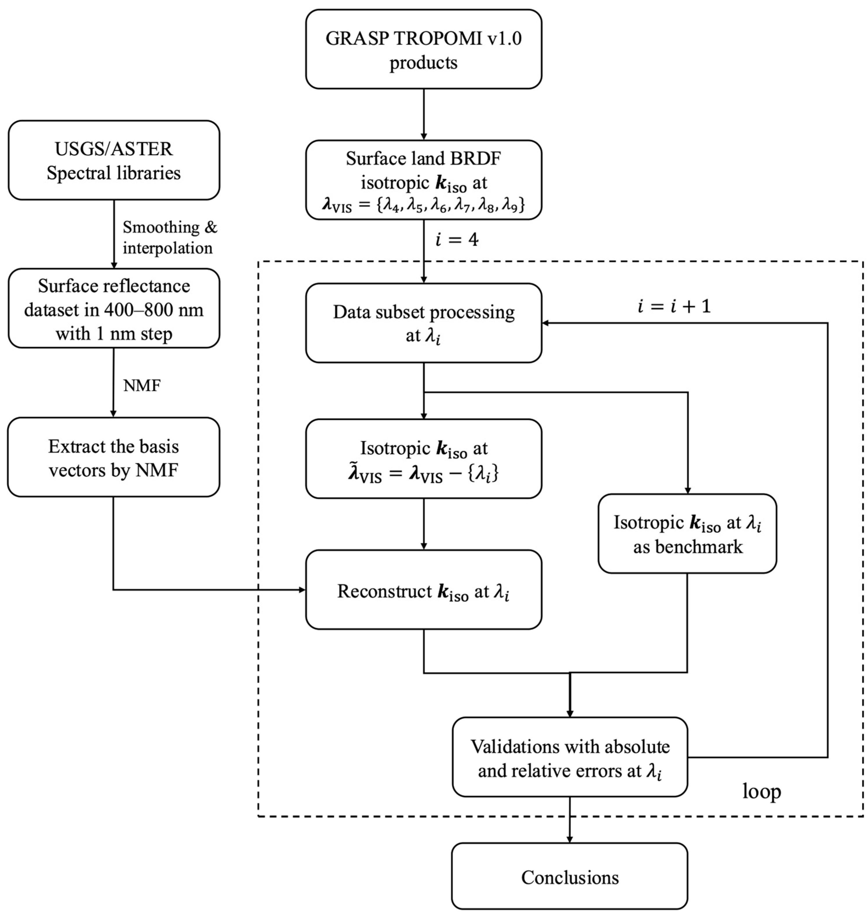
3.1. Flowchart of Research Strategy

Figure 1 shows the general flowchart for surface reflectance reconstruction in this study; the main steps include:

(1)

Using the USGS/ASTER spectral libraries as reference data for spectral analysis, we smooth and interpolate the surface reflectance dataset in the 400–800 nm range to encompass the visible (VIS) spectrum and part of the NIR, with a resolution of 1 nm per step. This interpolation process reduces noise, fills in missing values, and ensures a continuous dataset, enabling the capture of more detailed and accurate spectral information.

(2)

Basis vectors (endmember vectors) are extracted using non-negative matrix factorization (NMF) method, which is crucial for reducing dimensionality and finding meaningful patterns in the spectral dataset.

(3)

We select the wavelength-dependent isotropic parameters of land surface BRDF at six VIS and NIR wavelength bands from the GRASP TROPOMI v1.0 product for surface reflectance reconstruction. These wavelength bands are defined as:

$${\mathit{\lambda }}_{\mathrm{V}\mathrm{I}\mathrm{S}} = \left\{{\lambda }_4,{\lambda }_5,{\lambda }_6,{\lambda }_7,{\lambda }_8,{\lambda }_9\right\},$$

(5)

corresponding to 416, 440, 494, 670, 747, and 772 nm, respectively, from the GRASP TROPOMI BRDF product.

(4)

To quantitatively evaluate the effect of surface reflectance reconstruction, the selected isotropic coefficient dataset is dynamically divided into two subsets during each iteration of a loop. One subset,

$${\tilde{\mathit{\lambda }}}_{\mathrm{V}\mathrm{I}\mathrm{S}}={\mathit{\lambda }}_{\mathrm{V}\mathrm{I}\mathrm{S}} - \left\{{\lambda }_i\right\}, (i = 4,\cdots ,9),$$

(6)

is used to calculate the mixing coefficient vector $\mathit{h}$ for reconstructing the isotropic parameters at ${\lambda }_i$. The other subset, containing ${\lambda }_i$, serves as a benchmark to validate the reconstructed results by comparing absolute and relative errors.

(5)

By iterating through these six VIS and NIR wavelength bands in the loop, the accuracy of surface reflectance construction method can be systematically evaluated.

The BRDF isotropic parameters for wavelengths below 400 nm and above 800 nm can also be reconstructed using a similar surface reflectance reconstruction approach. However, this study primarily focuses on the wavelength range of 400–800 nm. Future research will aim to extend the spectral scope to include both UV and SWIR bands.

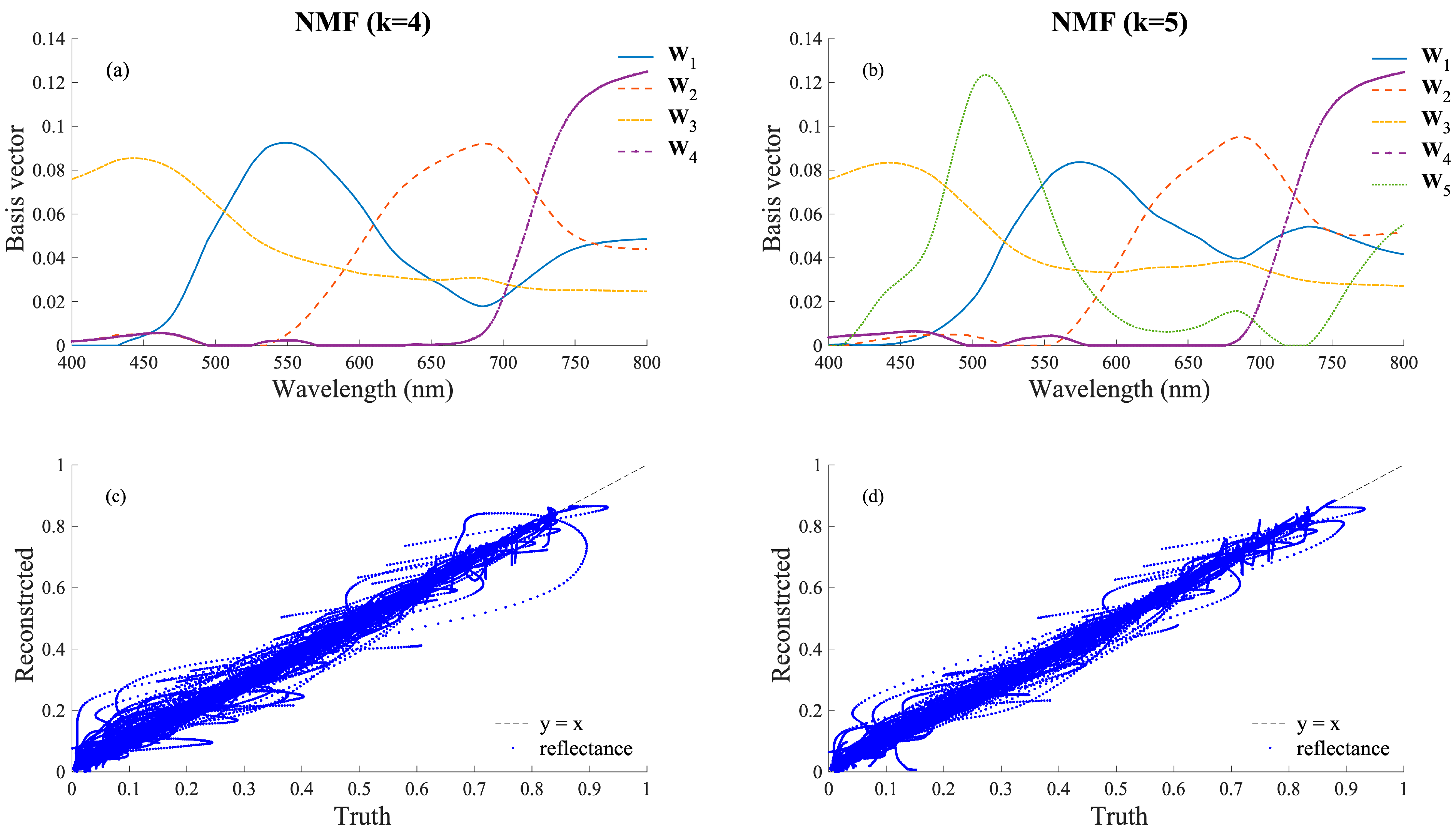
3.2. Extracted Basis Vectors

For a non-negative matrix $\mathit{V}\in R^{n\times m}$, representing hyperspectral or multispectral surface reflectance, NMF seek to decompose $\mathit{V}$ into two non-negative matrices $\mathit{W}\in R^{n\times k}$ and $\mathit{H}\in R^{k\times m}$, satisfying the factorization:

$$\mathit{V}\approx \mathit{W}\mathit{H},$$

(7)

where $n$ is the number of wavelength bands, $m$ is the number of spectra, and $k$ is desired rank with $k\ll \mathrm{m}\mathrm{i}\mathrm{n}\left(n,m\right)$.

By minimizing the difference between $\mathit{V}$ and $\mathit{W}\mathit{H}$, the conventional optimization for factorizing $\mathit{W}$ and $\mathit{H}$ is expressed as [33]

$$\begin{array}{c}min f(\mathit{W},\mathit{H}) = {\Vert \mathit{V} - \mathit{W}\mathit{H}\Vert }_F^2\hfill \\ s.t.\mathit{W}\ge 0, \mathit{H}\ge 0\hfill \end{array},$$

(8)

where ${\parallel \parallel }_F^2$ means the Frobenius norm and “s.t.” stands to “subject to”, indicating the non-negativity constraints on all elements of $\mathit{W}$ and $\mathit{H}$. Due to its nonsubtractive nature, NMF often provides a more intuitive and interpretable decomposition compared to PCA, especially in applications requiring non-negative basis vectors (column vectors of $\mathit{W}$).

Notably, NMF does not guarantee a unique solution for matrices $\mathit{W}$ and $\mathit{H}$ in Equation (8). If a full-rank square matrix $\mathit{X}$ (e.g., an orthogonal matrix) exists, $\mathit{V}$ can be equivalently expressed as:

$$\mathit{V}\approx \mathit{W}\mathit{X}{\mathit{X}}^{-1}\mathit{H},$$

(9)

with $\mathit{W}\mathit{X}\ge 0$ and ${\mathit{X}}^{-1}\mathit{H}\ge 0$. As a result, various algorithms have been developed to solve NMF stably, often incorporating additional constraints for specific applications, such as spectral unmixing. Section 1 has summarized several representative algorithms with their non-negativity constraints, including the BPAS-NMF method applied in this study [49].

Figure 2 illustrates the extracted basis vectors as a function of wavelength and scatterplot of reconstrued results with two different desired ranks ($k=4,5$) using the interpolated surface reflectance data from 400 nm to 800 nm with 1-nm step derived from the USGS/ASTER spectral libraries. For $k=4$, the mean absolute error (MAE) and mean relative error (MRE) of hyperspectral reflectance reconstruction are approximately 0.0050 and 3.71%, respectively, whereas increasing $k$ to 5 slightly reduces these errors to 0.0042 and 2.94%. By comprehensively considering the spectral shape and reconstruction performance in the visible range, we selected $k=4$ for surface reflectance reconstruction.

3.3. Surface Reflectance Reconstruciton

Using the extracted non-negative matrix $\mathit{W}$, composed by a few basis column vectors, any spectral vector $\mathit{r}$ can be reconstructed as a linear combination of these basis vectors [35,74]:

$$\mathit{r}\approx \mathit{W}\mathit{h},$$

(10)

where the details are expressed as

$$\left[\begin{array}{c}{r}_{{\lambda }_1}\\ ⋮\\ r_{{\lambda }_n}\end{array}\right]=\left[\begin{array}{ccc}{w}_{\mathrm{1,1}}& \cdots & w_{1,k}\\ ⋮& \ddots & ⋮\\ w_{n,1}& \cdots & w_{n,k}\end{array}\right]\left[\begin{array}{c}{h}_1\\ ⋮\\ h_k\end{array}\right].$$

(11)

This can also be written as

$$r_{{\lambda }_i}={\sum }_{j=1}^k{h}_j·w_{i,j}, i = 1,\cdots ,n,$$

(12)

where $\mathit{h}$ is the mixing coefficient vector and $r_{{\lambda }_i}$ represents the surface reflectance at the wavelength ${\lambda }_i$.

Once the basis matrix $\mathit{W}$ is determined, the surface reflectance spectra can be reconstructed if the mixing coefficient vector $\mathit{h}$ is known. Based on Equations (10)–(12), we have

$$\tilde{\mathit{r}}\approx \tilde{\mathit{W}} \mathit{h},$$

(13)

where

$$\left[\begin{array}{c}{r}_{d_1}\\ ⋮\\ r_{d_l}\end{array}\right]=\left[\begin{array}{ccc}{w}_{d_1,1}& \cdots & w_{d_1,k}\\ ⋮& \ddots & ⋮\\ w_{d_l,1}& \cdots & w_{d_l,k}\end{array}\right]\left[\begin{array}{c}{h}_1\\ ⋮\\ h_k\end{array}\right],\left(k\le l\right),$$

(14)

where $\tilde{\mathit{r}}$ represents a subset of $\mathit{r}$, $\tilde{\mathit{W}}$ is the corresponding subset of $\mathit{W}$ with the same number of columns, and $d_1,\cdots ,{\mathrm{a}\mathrm{n}\mathrm{d} d}_l$ denote a selected sequence of wavelength bands. The mixing coefficients vector $\mathit{h}$ can be approximately using a least-squares solution:

$$\mathit{h}\approx {\tilde{\mathit{W}}}^{+}\tilde{\mathit{r}},$$

(15)

where ${\tilde{\mathit{W}}}^{+}$ is a generalized inverse of $\tilde{\mathit{W}}$. If $k=l$, ${\tilde{\mathit{W}}}^{+}={\tilde{\mathit{W}}}^{-1}$.

After obtaining $\mathit{h}$, the isotropic coefficients spectral vector ${\mathit{k}}_{\mathbf{i}\mathbf{s}\mathbf{o}}^{\mathbf{r}\mathbf{e}\mathbf{c}}$ is reconstructed as

$${\mathit{k}}_{\mathbf{i}\mathbf{s}\mathbf{o}}^{\mathbf{r}\mathbf{e}\mathbf{c}}\approx \mathit{W}\mathit{h},$$

(16)

where ${\mathit{k}}_{\mathbf{i}\mathbf{s}\mathbf{o}}^{\mathbf{r}\mathbf{e}\mathbf{c}}={\left[k_{\mathrm{i}\mathrm{s}\mathrm{o}}^{\mathrm{r}\mathrm{e}\mathrm{c}}\left({\lambda }_1\right),\cdots ,k_{\mathrm{i}\mathrm{s}\mathrm{o}}^{\mathrm{r}\mathrm{e}\mathrm{c}}\left({\lambda }_n\right)\right]}^T$, and the superscript “$\mathrm{r}\mathrm{e}\mathrm{c}$” denote reconstructed results and $T$ means the transpose of a vector. Finally, the reconstructed BRDF ${\rho }_s^{\mathrm{r}\mathrm{e}\mathrm{c}}$ at any wavelength can be expressed as

$$\begin{array}{c}{\rho }_s^{\mathrm{r}\mathrm{e}\mathrm{c}}\left({\theta }_0,{\theta }_v,\phi ,{\lambda }_i\right) = k_{\mathrm{i}\mathrm{s}\mathrm{o}}^{\mathrm{r}\mathrm{e}\mathrm{c}}\left({\lambda }_i\right)[1 + k_{\mathrm{g}\mathrm{e}\mathrm{o}\mathrm{m}}{f}_{\mathrm{g}\mathrm{e}\mathrm{o}\mathrm{m}}\left({\theta }_0,{\theta }_v,\phi \right) + \\ k_{\mathrm{v}\mathrm{o}\mathrm{l}}{f}_{\mathrm{v}\mathrm{o}\mathrm{l}}\left({\theta }_0,{\theta }_v,\phi \right)], \left(i = 1,\cdots ,n\right).\end{array}$$

(17)

The reconstructed isotropic coefficients and corresponding BRDF results will be discussed the next section.

4. Results

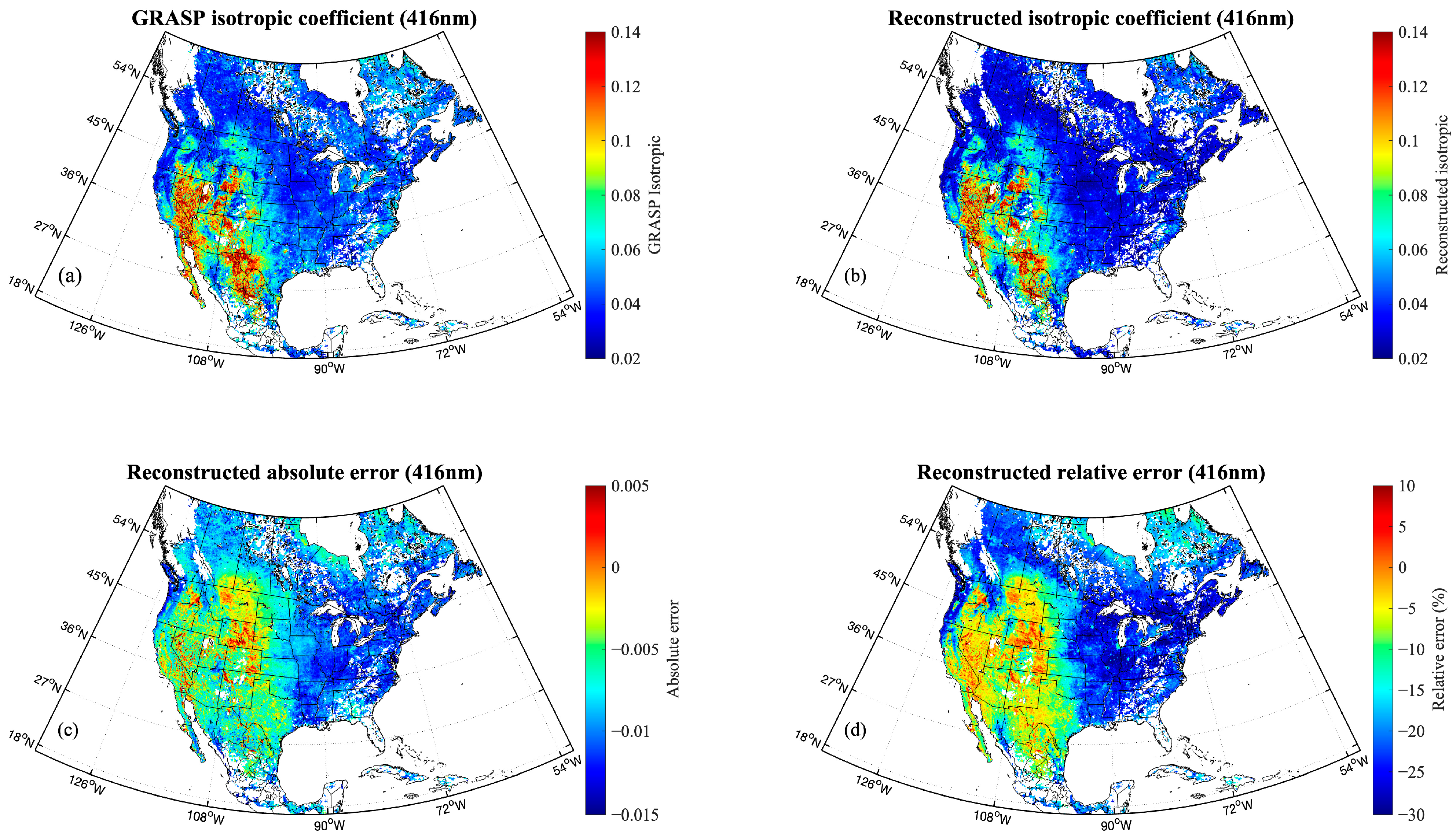
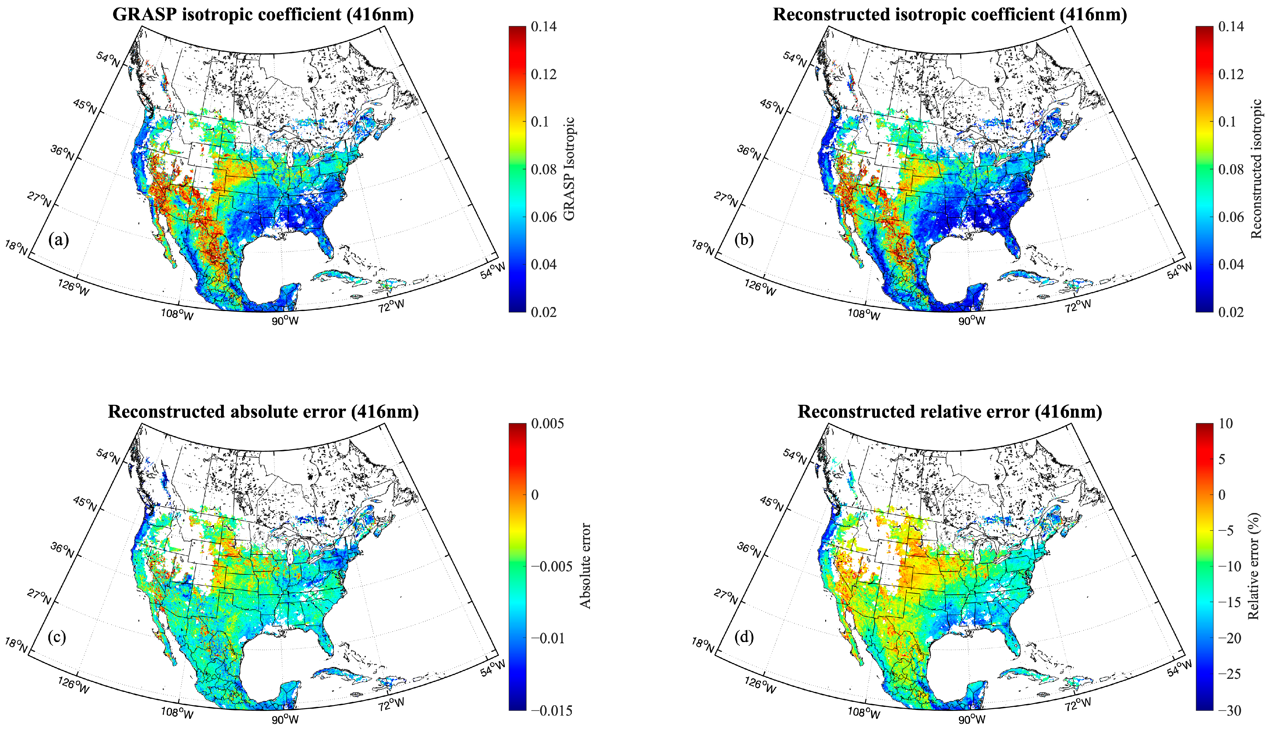
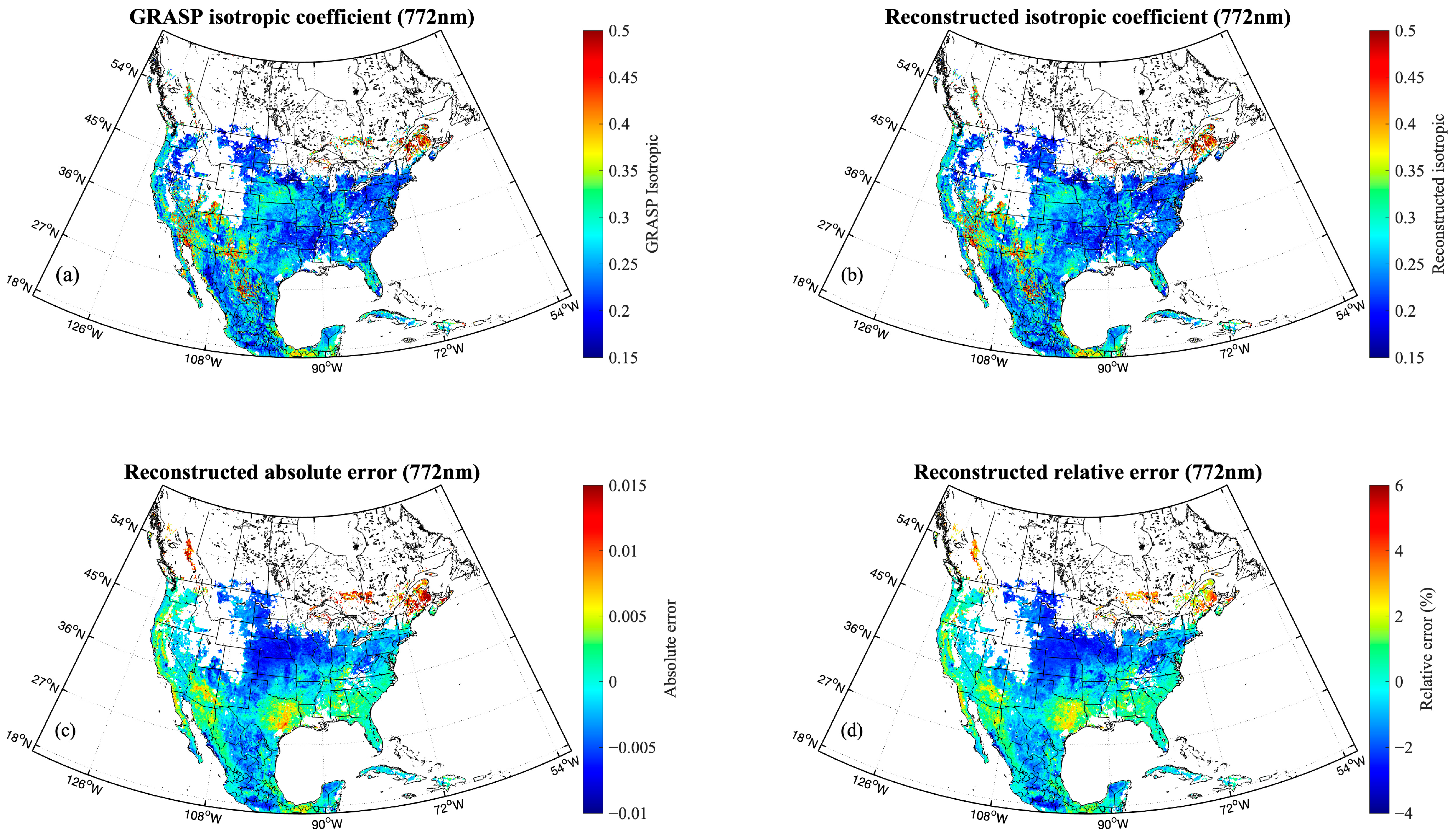
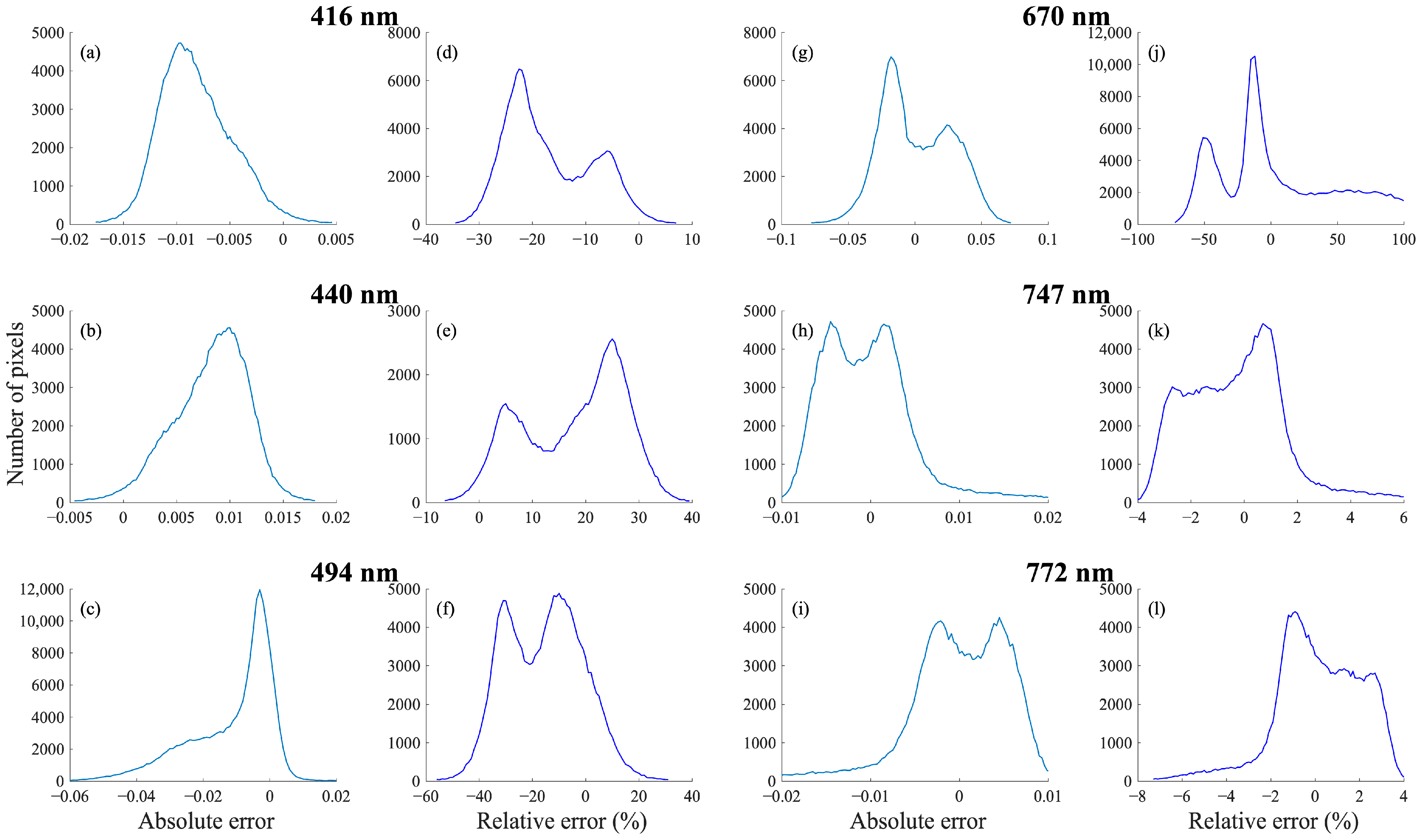
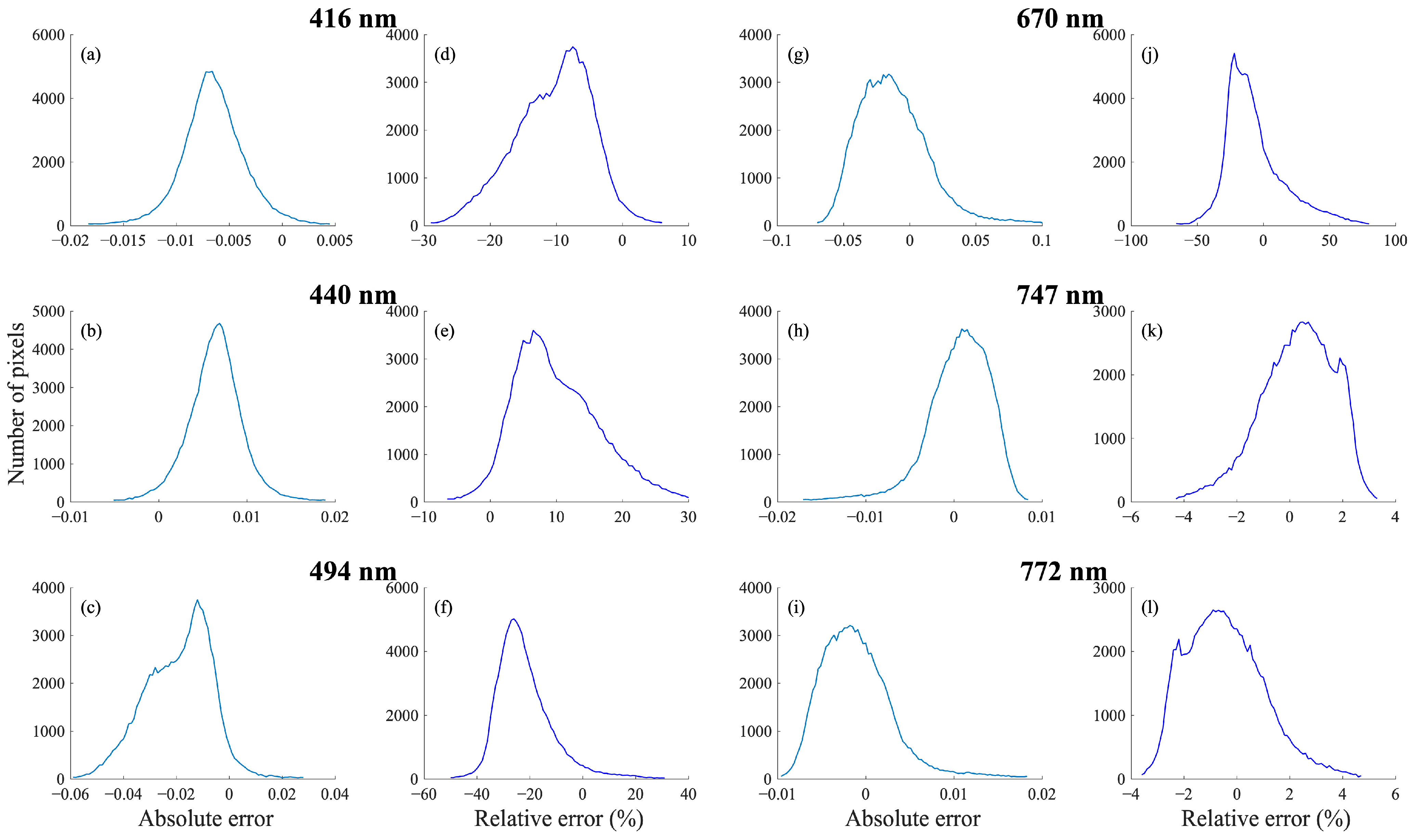
4.1. Reconstructed Spatial Distribution and Error Histogram

This section analyzes the spatial distribution and reconstruction accuracy of the BRDF isotropic coefficient at corresponding wavelengths using the monthly GRASP TROPOMI BRDF over North America for August and March 2020, respectively. Figure 3, Figure 4, Figure 5 and Figure 6 display the spatial maps of the GRASP isotropic coefficient, reconstructed isotropic coefficient, and their corresponding absolute and relative reconstruction errors at 416 nm and 772 nm. The reconstructions at 416 nm are based on five other wavelength bands (440, 494, 670, 747, and 772 nm) while the reconstruction at 772 nm is similarly based on five different wavelength bands (416, 440, 494, 670, and 747 nm). These figures demonstrate the performance of the reconstructed method in capturing the spatial distribution of surface BRDF isotropic coefficients.

Figure 7 and Figure 8 present histograms of absolute and relative errors for the six wavelengths during the same months, illustrating the statistical characteristics of reconstruction’s accuracy. In this analysis, the isotropic coefficient reconstructions at the designated wavelength band are derived using five other wavelength bands through NMF, ensuring that the specified wavelength is excluded from the spectral reconstruction process.

Table 2. Mean and standard deviation (Std. Dev.) of reconstructed absolute error and relative errors for the BRDF isotropic coefficients.

Data Date	Wavelength	Reconstructed Absolute Error		Reconstructed Relative Error
		Mean	Std. Dev.	Mean	Std. Dev.
August 2020	416 nm	−0.0080	0.0036	−16.62%	8.27%
	440 nm	0.0083	0.0037	18.04%	9.65%
	494 nm	−0.0039	0.0492	−4.45%	123.35%
	670 nm	0.0020	0.0273	16.39%	54.91%
	747 nm	0.0001	0.0057	−0.20%	1.94%
	772 nm	−0.0002	0.0065	0.20%	1.96%
March 2020	416 nm	−0.0065	0.0038	−10.22%	6.22%
	440 nm	0.0067	0.0040	10.47%	6.85%
	494 nm	−0.0141	0.0385	−21.96%	38.17%
	670 nm	−0.0092	0.0321	−4.93%	24.05%
	747 nm	0.0005	0.0042	0.33%	1.44%
	772 nm	−0.0007	0.0048	−0.38%	1.55%

shows that the reconstruction errors at 494 nm and 670 nm are notably higher compared to other wavelengths, both in terms of absolute and relative errors. For example, the relative error’s standard deviation at 494 nm in August 2020 reaches 123.35%, and at 670 nm, it is 54.91%, emphasizing the critical importance of these wavelengths for accurate reconstruction. These wavelengths capture key spectral features: 494 nm is associated with chlorophyll absorption and water content in vegetation, while 670 nm highlights red chlorophyll absorption. Both are essential for characterizing vegetation and surface properties. The exclusion of these wavelengths significantly increases reconstruction errors, thereby degrading accuracy in surface reflectance modeling. Consequently, 494 nm and 670 nm are indispensable for reliable surface reflectance reconstruction in this study, especially for vegetation and surface property studies. This does not, however, diminish the importance of other bands. Instead, it underscores the necessity of incorporating at least five bands of valid information. Attempts to perform surface reflectance reconstruction using only the first four bands (416, 440, 494, and 670 nm) or the last four bands (494, 670, 747, and 772 nm) still fall short of producing satisfactory reconstruction results.

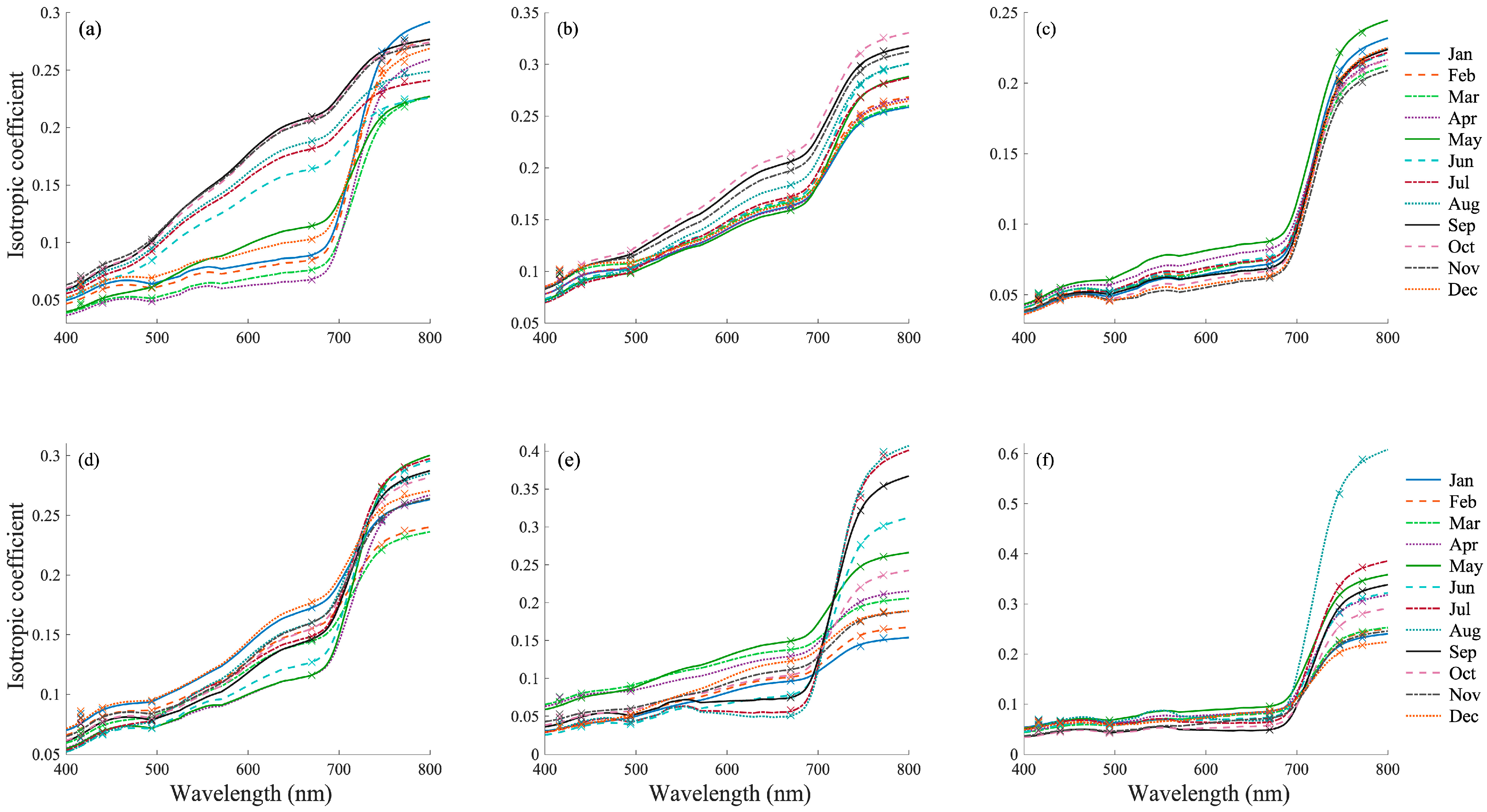
4.2. Reconstructed Spectral Features in the 400–800 nm Range

Figure 9 shows the monthly average spatial distribution of the reconstructed BRDF isotropic coefficient at 550 nm from January to December. The data from January to November are derived from the monthly average BRDF products of the corresponding months in 2020. For December, the monthly average BRDF product from December 2019 is used, as data for December 2020 are unavailable. These results derived using spectral reconstruction based on five wavelength bands (440, 494, 670, 747, and 772 nm) demonstrate the effectiveness of the NMF-based method across varying seasonal and spatial conditions. Due to the stringent quality control of the GRASP BRDF data, including the exclusion of pixels contaminated by snow, ice, and cloud, certain regions show missing data in different months, leading to spatial gaps in the reconstructed maps.

The reconstructed spatial distribution at 550 nm effectively reflects seasonal changes in isotropic coefficients across North America. Given that reflectance in the visible spectrum typically decreases as chlorophyll content increases [75], lower isotropic coefficients are observed during summer months (e.g., July–September) in vegetated areas, corresponding to decreased reflectance from active vegetation. Conversely, higher coefficients are seen in winter months (e.g., December–March), corresponding to reduced vegetation activity and potential snow cover. To further investigate spectral characteristics, six valid locations with consistent monthly data throughout the year are randomly selected for detailed analysis. This ensures representative results across varying seasons, highlighting the robustness of the reconstruction method.

Figure 10 illustrates the monthly spectral variations of the isotropic coefficient as a function of wavelength (400–800 nm) for six selected locations along 35.48°N, ranging from west to east. Panels (a) through (f) provide insights into monthly and seasonal variations across three key spectral regions: 550 nm (green band), 670 nm (red band), and the red-edge region (670–760 nm). These regions are critical for understanding vegetation dynamics.

At 550 nm, a prominent peak is observed in most panels, indicative of vegetation reflectance. Reflectance around 550 nm is relatively low in summer (e.g., June to September) across most panels, reflecting the peak growing season and increased chlorophyll content [75]. During fall and winter months (e.g., October to February), the reflectance increases due to reduced chlorophyll concentration and vegetation senescence.

At 670 nm, strong seasonal variations are evident. Reflectance is lowest in summer (e.g., June to August), corresponding to high chlorophyll absorption and active photosynthesis. In winter (e.g., December to February), reflectance increases due to reduced chlorophyll activity, indicating dormant vegetation or sparse canopy cover.

In the red-edge region (670–760 nm), reflectance increases sharply from red to NIR wavelengths, a phenomenon associated with vegetation’s cell structure and chlorophyll absorption. During summer, the red edge shifts toward longer wavelengths (e.g., closer to 750 nm), indicating high vegetation activity. In winter, the red edge shifts toward shorter wavelengths (e.g., around 700 nm), reflecting reduced vegetation activity. The red-edge slope, steepest in summer, signifies healthy vegetation with a high leaf area index (LAI) [76].

These seasonal and monthly variations reveal critical insights into vegetation phenology, including growth cycles, health, and stress detection. Patterns in these spectral regions can be used to compute vegetation indices such as NDVI, EVI, green NDVI (GNDVI), and the triangular vegetation index (TVI) for applications in agriculture, forestry, and environmental monitoring [68,77,78,79]. Thus, analyzing the 550 nm, 670 nm, and red-edge region provides a robust framework for understanding vegetation dynamics across temporal scales.

Figure 11 presents the spectral variations of reconstructed BRDF across different observation geometries at a selected location (90.88°W, 35.48°N) for 12 months, assuming 9:00 AM local time as an example. The BRDF is calculated using a combination of five view zenith angles (${\theta }_v$ = 0°, 20°, 40°, 60°, and 80°) and four relative azimuth angles ($\varphi$ = 0°, 60°, 120°, and 180°), while the solar zenith angle (${\theta }_0$) is predetermined based on the selected date, time, and geographical coordinates. Observation geometries significantly influence BRDF values. Higher view zenith angles (${\theta }_v$ = 60°, 80°) result in greater BRDF values, particularly in the near-infrared region. Relative azimuth angles ($\varphi$) modulate the reflectance values, with backscattering generally yielding higher BRDF compared to forward scattering.

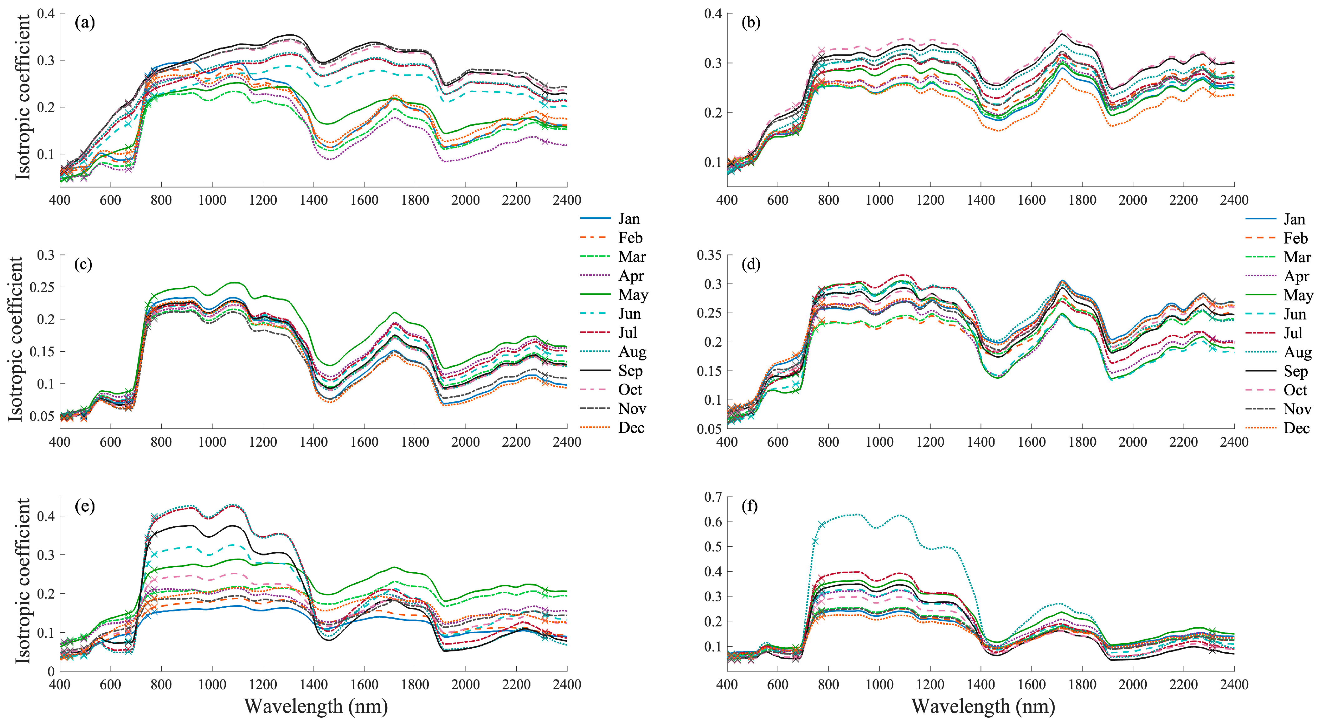
4.3. Reconstructed Spectral Features in the 400–2400 nm Range

To further demonstrate the general applicability and robustness of this proposed surface reflectance reconstruction method based on NMF, we incorporated BRDF data at the 2313 nm wavelength, extending the reconstructed spectral range from 400–800 nm to 400–2400 nm. Since the GRASP TROPOMI BRDF product provides only a single band in the SWIR (2313 nm), we do not evaluate the reconstruction accuracy of the BRDF isotropic coefficient parameters in this broader spectral range as in the earlier sections. Instead, we focus on showcasing the reconstructed spectral features.

Figure 12 illustrates the monthly spectral variations of the reconstructed BRDF isotropic coefficients across the spectral range of 400–2400 nm for the same six randomly selected locations listed in Figure 10. In the NIR (700–1400 nm), there is a sharp increase in reflectance, consistent with vegetation scattering properties, followed by distinct water absorption bands around 980 nm and 1200 nm [76,80]. In the SWIR spectral range (1400–2400 nm), multiple absorption features are present, influenced by water content, soil composition, and mineralogical characteristics [81,82,83]. The variation in depth and width of these absorption features suggests that the isotropic coefficients are sensitive to changes in biophysical and biochemical parameters, including leaf water content, surface moisture, and mineral abundance.

Figure 13 plots the spectral variations of the reconstructed BRDF across the spectral range of 400–2400 nm for different observation geometries. These results underline the robustness of the reconstructed BRDF, emphasizing the importance of incorporating detailed observation geometries and spectral characteristics for addressing spectral resolution gaps of surface reflectance. Notably, the results demonstrate effectiveness not only within the 400–800 nm but also across the broader spectral range of 400–2400 nm. The agreement between the reconstructed results and GRASP-derived values (cross symbols) further validates the effectiveness of the reconstruction approach.

To better interpret the spatial and spectral variations displayed in the figures above, it is essential to consider land cover types, topography, and seasonal changes as key influencing parameters. The reconstructed results, derived from the GRASP TROPOMI BRDF product, provide approximate spectral BRDF information, which facilitates the analysis of surface reflectance across diverse land cover types. However, to fully understand the spatial and temporal variations in surface reflectance, it is crucial to compare them with reference datasets, such as land cover classifications, digital elevation models (DEM), and seasonal vegetation indices (e.g., NDVI and EVI).

Figure 14 and Figure 15 depict the monthly average spatial distributions of NDVI and EVI across North America, derived from GRASP TROPOMI BRDF and the corresponding spectral reconstructions. Both indices exhibit a clear seasonal cycle, with lower values (blue regions) during winter months due to minimal vegetation activity and higher values (red regions) in summer, reflecting peak vegetation growth. During the transition months (e.g., April–May and September–October), vegetation indices gradually increase and decrease, capturing seasonal greening and senescence. The highest NDVI and EVI values are observed in the eastern U.S., central North America, and boreal forests of Canada, whereas arid and semiarid regions, such as the southwestern U.S. and northern Mexico, consistently show lower values. Compared to NDVI, EVI is more sensitive to variations in vegetation structure and density, particularly in sparsely vegetated areas, due to its reduced sensitivity to soil background and atmospheric effects [69,84]. These seasonal and spatial trends emphasize the importance of incorporating vegetation indices as key comparison parameters when analyzing BRDF variations, as they provide valuable insights into surface characteristics.

5. Discussion

The reconstruction of hyperspectral-like surface reflectance from multispectral datasets using NMF provides a complementary approach to address some challenges in remote sensing applications. One of the primary advantages lies in its ability to enhance the spectral reflectance information in specific bands, especially those impacted by strong atmospheric absorption or high atmospheric correction errors. By utilizing advanced reconstruction techniques, multispectral data with limited spectral resolution can be augmented to recover additional spectral information, thereby filling critical gaps in data coverage and improving surface feature differentiation [8,10,11,14,85,86].

It is essential to emphasize that this reconstruction approach is not intended to replace hyperspectral missions. Instead, it provides a cost-effective means to leverage the extensive spatial and temporal coverage offered by existing multispectral datasets, complementing hyperspectral observations. While hyperspectral sensors provide unparalleled spectral detail and accuracy, their high costs and computational demands limit their availability for large-scale and long-term monitoring [87,88]. Reconstruction methods using NMF offer a scalable alternative for augmenting multispectral data, particularly for applications requiring broader temporal coverage or in regions where hyperspectral data are unavailable.

Despite these advantages, several challenges and limitations require attention to ensure reliable application of spectral reconstruction. First, the quality of reconstruction is highly dependent on the accuracy and representativeness of the spectral libraries and prior knowledge. Fine spectral details that characterize hyperspectral data, such as subtle variations in absorption features, may not be fully recoverable, especially for complex surface compositions [11]. Refining spectral libraries and optimizing the extraction of spectral basis vectors through NMF are essential to enhance reconstruction performance.

Second, the generalizability of reconstruction models across diverse scenarios remains a key limitation. While NMF and other machine-learning-based methods provide flexibility in reconstructing spectral data, they may face difficulties when applied to heterogeneous surface conditions or spectral mixtures. Further optimization of these models, particularly through domain-specific constraints and adaptive algorithms, is crucial for expanding their applicability to diverse surface and atmospheric conditions [10,13].

Another critical challenge is the potential for noise and error propagation during the reconstruction process. Uncertainties or inaccuracies in the original multispectral data can be amplified, affecting the fidelity of the reconstructed reflectance. Effective quality control mechanisms, including the careful selection and preprocessing of high-quality multispectral datasets, are necessary to minimize such errors and improve the robustness of the results [8,9].

In short, the spectral reconstruction of land surface reflectance using NMF offers a promising avenue for augmenting spectral information in multispectral datasets. This approach is particularly valuable for addressing limitations in certain spectral bands and for scenarios where high-resolution hyperspectral observations are impractical or unavailable. Continued advancements in spectral library refinement, modeling techniques, and data quality assurance are expected to further enhance the reliability and applicability of surface reflectance reconstruction methods, ensuring their role as a complementary tool in remote sensing.

6. Conclusions

This study presents an approach for enhancing multispectral surface reflectance data by reconstructing additional spectral information, focusing on the spectral range of 400–800 nm using the GRASP TROPOMI BRDF product. Using non-negative matrix factorization (NMF), spectral basis vectors were extracted from reference spectral libraries, enabling the reconstruction of key spectral features with a few limited wavelength bands. The results demonstrate the effectiveness of this approach in complementing multispectral data by enhancing spectral information at specific wavelengths, particularly those affected by strong atmospheric absorption or significant atmospheric correction errors.

The analysis draws attention to the critical role of specific wavelengths, such as 494 nm and 670 nm, in reconstructing spectral features due to their sensitivity to vegetation reflectance and chlorophyll absorption, emphasizing that at least five bands of valid information are necessary for relative reliable results in the spectral range of 400–800 nm. Moreover, by incorporating BRDF data at 2313 nm, the method extends its applicability across the broader spectral range of 400–2400 nm, effectively bridging spectral resolution gaps of multispectral surface reflectance. The reconstructed BRDF results not only closely agree with the GRASP BRDF product but also demonstrate the robustness and reliability of this approach for applications requiring comprehensive and reliable surface reflectance information.

This framework demonstrates the potential to enhance multispectral datasets by filling critical spectral gaps, offering a cost-effective and scalable solution for large-scale remote sensing applications. However, it is not intended to replace hyperspectral data but rather to supplement existing multispectral observations, particularly in scenarios where hyperspectral missions are impractical or unavailable.

In conclusion, this study contributes to advancing spectral reconstruction methods for land surface analysis. Future research will focus on refining spectral libraries, improving reconstruction accuracy, and extending applications across broader spectral ranges from UV to SWIR. These efforts aim to further enhance the reliability and applicability of this approach, supporting more accurate and comprehensive surface characterization.

References

1. Macarringue, L.S.; Bolfe, É.L.; Pereira, P.R.M. Developments in land use and land cover classification techniques in remote sensing: A review. J. Geogr. Inf. Syst. 2022, 14, 1–28. [Google Scholar] [CrossRef]
2. Atzberger, C. Advances in remote sensing of agriculture: Context description, existing operational monitoring systems and major information needs. Remote Sens. 2013, 5, 949–981. [Google Scholar] [CrossRef]
3. Li, J.; Pei, Y.; Zhao, S.; Xiao, R.; Sang, X.; Zhang, C. A review of remote sensing for environmental monitoring in China. Remote Sens. 2020, 12, 1130. [Google Scholar] [CrossRef]
4. Liu, Y.; Wang, Z.; Sun, Q.; Erb, A.M.; Li, Z.; Schaaf, C.B.; Zhang, X.; Román, M.O.; Scott, R.L.; Zhang, Q.; et al. Evaluation of the VIIRS BRDF, Albedo and NBAR products suite and an assessment of continuity with the long term MODIS record. Remote Sens. Environ. 2017, 201, 256–274. [Google Scholar] [CrossRef]
5. Claverie, M.; Vermote, E.F.; Franch, B.; Masek, J.G. Evaluation of the Landsat-5 TM and Landsat-7 ETM+ surface reflectance products. Remote Sens. Environ. 2015, 169, 390–403. [Google Scholar] [CrossRef]
6. Chen, C.; Dubovik, O.; Fuertes, D.; Litvinov, P.; Lapyonok, T.; Lopatin, A.; Ducos, F.; Derimian, Y.; Herman, M.; Tanré, D.; et al. Validation of GRASP algorithm product from POLDER/PARASOL data and assessment of multi-angular polarimetry potential for aerosol monitoring. Earth Syst. Sci. Data 2020, 12, 3573–3620. [Google Scholar] [CrossRef]
7. Zhang, H.; Kondragunta, S.; Laszlo, I.; Zhou, M. Improving GOES Advanced Baseline Imager (ABI) aerosol optical depth (AOD) retrievals using an empirical bias correction algorithm. Atmos. Meas. Tech. 2020, 13, 5955–5975. [Google Scholar] [CrossRef]
8. Wang, W.; Dungan, J.; Genovese, V.; Shinozuka, Y.; Yang, Q.; Liu, X.; Poulter, B.; Brosnan, I. Development of the Ames Global Hyperspectral Synthetic Data Set: Surface Bidirectional Reflectance Distribution Function. J. Geophys. Res. Biogeosci. 2023, 128, e2022JG007363. [Google Scholar] [CrossRef]
9. Yang, Q.; Liu, X.; Wu, W. A Hyperspectral Bidirectional Reflectance Model for Land Surface. Sensors 2020, 20, 4456. [Google Scholar] [CrossRef]
10. Li, Z.; Sun, D.; Qiu, Z.; Xi, H.; Wang, S.; Perrie, W.; Li, Y.; Han, B. A Reconstruction Method for Hyperspectral Remote Sensing Reflectance in the Visible Domain and Applications. J. Geophys. Res. Ocean. 2018, 123, 4092–4109. [Google Scholar] [CrossRef]
11. Roccetti, G.; Bugliaro, L.; Gödde, F.; Emde, C.; Hamann, U.; Manev, M.; Sterzik, M.F.; Wehrum, C. HAMSTER: Hyperspectral Albedo Maps dataset with high Spatial and TEmporal Resolution. Atmos. Meas. Tech. 2024, 17, 6025–6046. [Google Scholar] [CrossRef]
12. Ahmed, M.T.; Villordon, A.; Kamruzzaman, M. Comparative analysis of hyperspectral Image reconstruction using deep learning for agricultural and biological applications. Results Eng. 2024, 23, 102623. [Google Scholar] [CrossRef]
13. Zhang, J.; Su, R.; Fu, Q.; Ren, W.; Heide, F.; Nie, Y. A survey on computational spectral reconstruction methods from RGB to hyperspectral imaging. Sci. Rep. 2022, 12, 11905. [Google Scholar] [CrossRef] [PubMed]
14. Deng, L.; Sun, J.; Chen, Y.; Lu, H.; Duan, F.; Zhu, L.; Fan, T. M2H-Net: A reconstruction method for hyperspectral remotely sensed imagery. ISPRS J. Photogramm. Remote Sens. 2021, 173, 323–348. [Google Scholar] [CrossRef]
15. Zhao, E.; Qu, N.; Wang, Y.; Gao, C. Spectral Reconstruction from Thermal Infrared Multispectral Image Using Convolutional Neural Network and Transformer Joint Network. Remote Sens. 2024, 16, 1284. [Google Scholar] [CrossRef]
16. Shen, H.-L.; Cai, P.-Q.; Shao, S.-J.; Xin, J.H. Reflectance reconstruction for multispectral imaging by adaptive Wiener estimation. Opt. Express 2007, 15, 15545–15554. [Google Scholar] [CrossRef]
17. Zhang, X.; Cui, G.; Ruan, X.; Cui, D.; Gao, X.; Chen, Q.; Yao, Y.; Melgosa, M.; Sueeprasan, S. Spectral reflectance reconstruction based on wideband multi-illuminant imaging and a modified particle swarm optimization algorithm. Opt. Express 2024, 32, 2942–2958. [Google Scholar] [CrossRef]
18. Yao, P.; Wu, H.; Xin, J.H. Improving Generalizability of Spectral Reflectance Reconstruction Using L1-Norm Penalization. Sensors 2023, 23, 689. [Google Scholar] [CrossRef]
19. Zoogman, P.; Liu, X.; Chance, K.; Sun, Q.; Schaaf, C.; Mahr, T.; Wagner, T. A climatology of visible surface reflectance spectra. J. Quant. Spectrosc. Radiat. Transf. 2016, 180, 39–46. [Google Scholar] [CrossRef]
20. Yu, W.; Li, J.; Liu, Q.; Zeng, Y.; Zhao, J.; Xu, B.; Yin, G. Global Land Cover Heterogeneity Characteristics at Moderate Resolution for Mixed Pixel Modeling and Inversion. Remote Sens. 2018, 10, 856. [Google Scholar] [CrossRef]
21. Bioucas-Dias, J.M.; Plaza, A.; Dobigeon, N.; Parente, M.; Du, Q.; Gader, P.; Chanussot, J. Hyperspectral Unmixing Overview: Geometrical, Statistical, and Sparse Regression-Based Approaches. IEEE J. Sel. Top. Appl. Earth Obs. Remote Sens. 2012, 5, 354–379. [Google Scholar] [CrossRef]
22. Du, P.; Liu, S.; Liu, P.; Tan, K.; Cheng, L. Sub-pixel change detection for urban land-cover analysis via multi-temporal remote sensing images. Geo-Spat. Inf. Sci. 2014, 17, 26–38. [Google Scholar] [CrossRef]
23. Hu, Z.; Chu, Y.; Zhang, Y.; Zheng, X.; Wang, J.; Xu, W.; Wang, J.; Wu, G. Scale matters: How spatial resolution impacts remote sensing based urban green space mapping? Int. J. Appl. Earth Obs. Geoinf. 2024, 134, 104178. [Google Scholar] [CrossRef]
24. Clark, R.N.; Swayze, G.A.; Livo, K.E.; Kokaly, R.F.; King, T.V.; Dalton, J.B.; Vance, J.S.; Rockwell, B.W.; Hoefen, T.; McDougal, R.R. Surface reflectance calibration of terrestrial imaging spectroscopy data: A tutorial using AVIRIS. In Proceedings of the 10th Airborne Earth Science Workshop, Pasadena, CA, USA, 27 February–2 March 2001. [Google Scholar]
25. Song, X.; Zou, L.; Wu, L. Detection of Subpixel Targets on Hyperspectral Remote Sensing Imagery Based on Background Endmember Extraction. IEEE Trans. Geosci. Remote Sens. 2021, 59, 2365–2377. [Google Scholar] [CrossRef]
26. Miao, L.; Qi, H. Endmember Extraction From Highly Mixed Data Using Minimum Volume Constrained Nonnegative Matrix Factorization. IEEE Trans. Geosci. Remote Sens. 2007, 45, 765–777. [Google Scholar] [CrossRef]
27. Fan, F.; Deng, Y. Enhancing endmember selection in multiple endmember spectral mixture analysis (MESMA) for urban impervious surface area mapping using spectral angle and spectral distance parameters. Int. J. Appl. Earth Obs. Geoinf. 2014, 33, 290–301. [Google Scholar] [CrossRef]
28. Gómez-Sánchez, A.; Marro, M.; Marsal, M.; Zacchetti, S.; Rocha de Oliveira, R.; Loza-Alvarez, P.; de Juan, A. Linear unmixing protocol for hyperspectral image fusion analysis applied to a case study of vegetal tissues. Sci. Rep. 2021, 11, 18665. [Google Scholar] [CrossRef]
29. Févotte, C.; Dobigeon, N. Nonlinear Hyperspectral Unmixing With Robust Nonnegative Matrix Factorization. IEEE Trans. Image Process. 2015, 24, 4810–4819. [Google Scholar] [CrossRef]
30. Rajabi, R.; Ghassemian, H. Spectral Unmixing of Hyperspectral Imagery Using Multilayer NMF. IEEE Geosci. Remote Sens. Lett. 2015, 12, 38–42. [Google Scholar] [CrossRef]
31. Akhtar, N.; Mian, A. RCMF: Robust Constrained Matrix Factorization for Hyperspectral Unmixing. IEEE Trans. Geosci. Remote Sens. 2017, 55, 3354–3366. [Google Scholar] [CrossRef]
32. Liu, R.; Du, B.; Zhang, L. Hyperspectral Unmixing via Double Abundance Characteristics Constraints Based NMF. Remote Sens. 2016, 8, 464. [Google Scholar] [CrossRef]
33. Lee, D.D.; Seung, H.S. Learning the parts of objects by non-negative matrix factorization. Nature 1999, 6755, 788–791. [Google Scholar] [CrossRef]
34. Fathi Hafshejani, S.; Moaberfard, Z. Initialization for non-negative matrix factorization: A comprehensive review. Int. J. Data Sci. Anal. 2023, 16, 119–134. [Google Scholar] [CrossRef]
35. Hou, W.; Wang, J.; Xu, X.; Reid, J.S.; Han, D. An algorithm for hyperspectral remote sensing of aerosols: 1. Development of theoretical framework. J. Quant. Spectrosc. Radiat. Transf. 2016, 178, 400–415. [Google Scholar] [CrossRef]
36. Hou, W.; Wang, J.; Xu, X.; Reid, J.S.; Janz, S.J.; Leitch, J.W. An algorithm for hyperspectral remote sensing of aerosols: 3. Application to the GEO-TASO data in KORUS-AQ field campaign. J. Quant. Spectrosc. Radiat. Transf. 2020, 253, 107161. [Google Scholar] [CrossRef]
37. Hou, W.; Mao, Y.; Xu, C.; Li, Z.; Li, D.; Ma, Y.; Xu, H. Study on the spectral reconstruction of typical surface types based on spectral library and principal component analysis. SPIE 2019, 11023, 702–711. [Google Scholar]
38. Ferrero, A.; Campos, J.; Rabal, A.M.; Pons, A.; Hernanz, M.L.; Corróns, A. Principal components analysis on the spectral bidirectional reflectance distribution function of ceramic colour standards. Opt. Express 2011, 19, 19199–19211. [Google Scholar] [CrossRef]
39. Hou, W.; Wang, J.; Xu, X.; Reid, J.S. An algorithm for hyperspectral remote sensing of aerosols: 2. Information content analysis for aerosol parameters and principal components of surface spectra. J. Quant. Spectrosc. Radiat. Transf. 2017, 192, 14–29. [Google Scholar] [CrossRef]
40. Pauca, V.P.; Piper, J.; Plemmons, R.J. Nonnegative matrix factorization for spectral data analysis. Linear Algebra Its Appl. 2006, 416, 29–47. [Google Scholar] [CrossRef]
41. Hassani, A.; Iranmanesh, A.; Mansouri, N. Text mining using nonnegative matrix factorization and latent semantic analysis. Neural Comput. Appl. 2021, 33, 13745–13766. [Google Scholar] [CrossRef]
42. Qian, Y.; Jia, S.; Zhou, J.; Robles-Kelly, A. Hyperspectral Unmixing via L1/2 Sparsity-Constrained Nonnegative Matrix Factorization. IEEE Trans. Geosci. Remote Sens. 2011, 49, 4282–4297. [Google Scholar] [CrossRef]
43. Feng, X.-R.; Li, H.-C.; Wang, R.; Du, Q.; Jia, X.; Plaza, A. Hyperspectral unmixing based on nonnegative matrix factorization: A comprehensive review. IEEE J. Sel. Top. Appl. Earth Obs. Remote Sens. 2022, 15, 4414–4436. [Google Scholar] [CrossRef]
44. Lee, D.; Seung, H.S. Algorithms for non-negative matrix factorization. Adv. Neural Inf. Process. Syst. 2000, 13. [Google Scholar]
45. Lin, C.-J. Projected Gradient Methods for Nonnegative Matrix Factorization. Neural Comput. 2007, 19, 2756–2779. [Google Scholar] [CrossRef]
46. Kim, H.; Park, H. Sparse non-negative matrix factorizations via alternating non-negativity-constrained least squares for microarray data analysis. Bioinformatics 2007, 23, 1495–1502. [Google Scholar] [CrossRef] [PubMed]
47. Kim, H.; Park, H. Nonnegative Matrix Factorization Based on Alternating Nonnegativity Constrained Least Squares and Active Set Method. SIAM J. Matrix Anal. Appl. 2008, 30, 713–730. [Google Scholar] [CrossRef]
48. Kim, J.; Park, H. Toward Faster Nonnegative Matrix Factorization: A New Algorithm Comparisons. In Proceedings of the 2008 Eighth IEEE International Conference on Data Mining, Pisa, Italy, 15–19 December 2008; pp. 353–362. [Google Scholar] [CrossRef]
49. Kim, J.; Park, H. Fast Nonnegative Matrix Factorization: An Active-Set-Like Method and Comparisons. SIAM J. Sci. Comput. 2011, 33, 3261–3281. [Google Scholar] [CrossRef]
50. Cichocki, A.; Zdunek, R. Regularized alternating least squares algorithms for non-negative matrix/tensor factorization. In Advances in Neural Network—ISNN 2007; Springer: Berlin/Heidelberg, Germany, 2007; pp. 793–802. [Google Scholar]
51. Hoyer, P.O. Non-negative matrix factorization with sparseness constraints. J. Mach. Learn. Res. 2004, 5, 1457–1469. [Google Scholar]
52. Gillis, N.; Glineur, F. Using underapproximations for sparse nonnegative matrix factorization. Pattern Recognit. 2010, 43, 1676–1687. [Google Scholar] [CrossRef]
53. Schmidt, M.N.; Winther, O.; Hansen, L.K. Bayesian non-negative matrix factorization. In Proceedings of the Independent Component Analysis and Signal Separation: 8th International Conference, ICA 2009, Paraty, Brazil, 15–18 March 2009; Proceedings 8. pp. 540–547. [Google Scholar]
54. Zafeiriou, S.; Tefas, A.; Buciu, I.; Pitas, I. Exploiting discriminant information in nonnegative matrix factorization with application to frontal face verification. IEEE Trans. Neural Netw. 2006, 17, 683–695. [Google Scholar] [CrossRef]
55. Zhang, D.; Zhou, Z.-H.; Chen, S. Non-negative matrix factorization on kernels. In Proceedings of the PRICAI 2006: Trends in Artificial Intelligence: 9th Pacific Rim International Conference on Artificial Intelligence, Guilin, China, 7–11 August 2006; Proceedings 9. pp. 404–412. [Google Scholar]
56. Liu, H.; Wu, Z. Non-negative matrix factorization with constraints. In Proceedings of the AAAI Conference on Artificial Intelligence, Atlanta, GA, USA, 11–15 July 2010; pp. 506–511. [Google Scholar]
57. Li, J.; Bioucas-Dias, J.M.; Plaza, A.; Liu, L. Robust Collaborative Nonnegative Matrix Factorization for Hyperspectral Unmixing. IEEE Trans. Geosci. Remote Sens. 2016, 54, 6076–6090. [Google Scholar] [CrossRef]
58. Wang, Y.-X.; Zhang, Y.-J. Nonnegative matrix factorization: A comprehensive review. IEEE Trans. Knowl. Data Eng. 2012, 25, 1336–1353. [Google Scholar] [CrossRef]
59. Gillis, N. The why and how of nonnegative matrix factorization. Regul. Optim. Kernels Support Vector Mach. 2014, 12, 257–291. [Google Scholar]
60. Dubovik, O.; Lapyonok, T.; Litvinov, P.; Herman, M.; Fuertes, D.; Ducos, F.; Torres, B.; Derimian, Y.; Huang, X.; Lopatin, A.; et al. GRASP: A versatile algorithm for characterizing the atmosphere. SPIE Newsroom 2014, 25, 2-1201408. [Google Scholar] [CrossRef]
61. Torres, B.; Dubovik, O.; Fuertes, D.; Schuster, G.; Cachorro, V.E.; Lapionak, T.; Goloub, P.; Blarel, L.; Barreto, A.; Mallet, M.; et al. Advanced characterization of aerosol properties from measurements of spectral optical depth using the GRASP algorithm. Atmos. Meas. Tech. Discuss. 2016, 10, 3743–3781. [Google Scholar] [CrossRef]
62. Dubovik, O.; Fuertes, D.; Litvinov, P.; Lopatin, A.; Lapyonok, T.; Doubovik, I.; Xu, F.; Ducos, F.; Chen, C.; Torres, B.; et al. A Comprehensive Description of Multi-Term LSM for Applying Multiple a Priori Constraints in Problems of Atmospheric Remote Sensing: GRASP Algorithm, Concept, and Applications. Front. Remote Sens. 2021, 2, 706851. [Google Scholar] [CrossRef]
63. Litvinov, P.; Chen, C.; Dubovik, O.; Bindreiter, L.; Matar, C.; Fuertes, D.; Lopatin, A.; Lapyonok, T.; Lanzinger, V.; Hangler, A.; et al. Extended aerosol and surface characterization from S5P/TROPOMI with GRASP algorithm. Part I: Conditions, approaches, performance and new possibilities. Remote Sens. Environ. 2024, 313, 114355. [Google Scholar] [CrossRef]
64. Chen, C.; Litvinov, P.; Dubovik, O.; Bindreiter, L.; Matar, C.; Fuertes, D.; Lopatin, A.; Lapyonok, T.; Lanzinger, V.; Hangler, A.; et al. Extended aerosol and surface characterization from S5P/TROPOMI with GRASP algorithm. Part II: Global validation and Intercomparison. Remote Sens. Environ. 2024, 313, 114374. [Google Scholar] [CrossRef]
65. Chen, C.; Litvinov, P.; Dubovik, O.; Fuertes, D.; Matar, C.; Miglietta, F.; Pepe, M.; Genesio, L.; Busetto, L.; Bindreiter, L.; et al. Retrieval of aerosol and surface properties at high spatial resolution: Hybrid approach and demonstration using sentinel-5p/TROPOMI and PRISMA. J. Geophys. Res. Atmos. 2024, 129, e2024JD041041. [Google Scholar] [CrossRef]
66. Veefkind, J.P.; Aben, I.; McMullan, K.; Förster, H.; De Vries, J.; Otter, G.; Claas, J.; Eskes, H.; De Haan, J.; Kleipool, Q.; et al. TROPOMI on the ESA Sentinel-5 Precursor: A GMES mission for global observations of the atmospheric composition for climate, air quality and ozone layer applications. Remote Sens. Environ. 2012, 120, 70–83. [Google Scholar] [CrossRef]
67. Litvinov, P.; Hasekamp, O.; Cairns, B. Models for surface reflection of radiance and polarized radiance: Comparison with airborne multi-angle photopolarimetric measurements and implications for modeling top-of-atmosphere measurements. Remote Sens. Environ. 2011, 115, 781–792. [Google Scholar] [CrossRef]
68. Huete, A.; Didan, K.; Miura, T.; Rodriguez, E.P.; Gao, X.; Ferreira, L.G. Overview of the radiometric and biophysical performance of the MODIS vegetation indices. Remote Sens. Environ. 2002, 83, 195–213. [Google Scholar] [CrossRef]
69. Waring, R.; Coops, N.; Fan, W.; Nightingale, J. MODIS enhanced vegetation index predicts tree species richness across forested ecoregions in the contiguous USA. Remote Sens. Environ. 2006, 103, 218–226. [Google Scholar] [CrossRef]
70. Matsushita, B.; Yang, W.; Chen, J.; Onda, Y.; Qiu, G. Sensitivity of the enhanced vegetation index (EVI) and normalized difference vegetation index (NDVI) to topographic effects: A case study in high-density cypress forest. Sensors 2007, 7, 2636–2651. [Google Scholar] [CrossRef]
71. Kokaly, R.F.; Clark, R.N.; Swayze, G.A.; Livo, K.E.; Hoefen, T.M.; Pearson, N.C.; Wise, R.A.; Benzel, W.M.; Lowers, H.A.; Driscoll, R.L.; et al. USGS Spectral Library Version 7; 1035; U.S. Geological Survey: Reston, VA, USA, 2017; p. 68.
72. Baldridge, A.M.; Hook, S.J.; Grove, C.I.; Rivera, G. The ASTER spectral library version 2.0. Remote Sens. Environ. 2009, 113, 711–715. [Google Scholar] [CrossRef]
73. Sridhar, M.; Muthukumar, M. Spectral Library for Various Rocks and Minerals of Salem District: A Comparative Study and Validation with ASTER Data. In On a Sustainable Future of the Earth’s Natural Resources; Ramkumar, M., Ed.; Springer: Berlin/Heidelberg, Germany, 2013; pp. 149–157. [Google Scholar]
74. Hou, W.; Li, Z.; Dong, X.; Zhou, Z.; Ge, B.; Zheng, Y.; Yao, Q.; Fan, C.; Shi, Z. Hyperspectral surface reflectance reconstruction based on non-negative matrix factorization and multispectral results. Proc. SPIE 2021, 12064, 86–92. [Google Scholar] [CrossRef]
75. Yang, Y.; Nan, R.; Mi, T.; Song, Y.; Shi, F.; Liu, X.; Wang, Y.; Sun, F.; Xi, Y.; Zhang, C. Rapid and Nondestructive Evaluation of Wheat Chlorophyll under Drought Stress Using Hyperspectral Imaging. Int. J. Mol. Sci. 2023, 24, 5825. [Google Scholar] [CrossRef]
76. Fang, H.; Baret, F.; Plummer, S.; Schaepman-Strub, G. An Overview of Global Leaf Area Index (LAI): Methods, Products, Validation, and Applications. Rev. Geophys. 2019, 57, 739–799. [Google Scholar] [CrossRef]
77. Hunt, E.R.; Doraiswamy, P.C.; McMurtrey, J.E.; Daughtry, C.S.T.; Perry, E.M.; Akhmedov, B. A visible band index for remote sensing leaf chlorophyll content at the canopy scale. Int. J. Appl. Earth Obs. Geoinf. 2013, 21, 103–112. [Google Scholar] [CrossRef]
78. Galieni, A.; D’Ascenzo, N.; Stagnari, F.; Pagnani, G.; Xie, Q.; Pisante, M. Past and Future of Plant Stress Detection: An Overview From Remote Sensing to Positron Emission Tomography. Front. Plant Sci. 2021, 11, 609155. [Google Scholar] [CrossRef]
79. Qian, B.; Ye, H.; Huang, W.; Xie, Q.; Pan, Y.; Xing, N.; Ren, Y.; Guo, A.; Jiao, Q.; Lan, Y. A sentinel-2-based triangular vegetation index for chlorophyll content estimation. Agric. For. Meteorol. 2022, 322, 109000. [Google Scholar] [CrossRef]
80. Bell, I.E.; Baranoski, G.V.G. Reducing the dimensionality of plant spectral databases. IEEE Trans. Geosci. Remote Sens. 2004, 42, 570–576. [Google Scholar] [CrossRef]
81. Fabre, S.; Briottet, X.; Lesaignoux, A. Estimation of Soil Moisture Content from the Spectral Reflectance of Bare Soils in the 0.4–2.5 µm Domain. Sensors 2015, 15, 3262–3281. [Google Scholar] [CrossRef]
82. Govender, M.; Chetty, K.; Bulcock, H. A review of hyperspectral remote sensing and its application in vegetation and water resource studies. Water Sa 2007, 33, 145–151. [Google Scholar] [CrossRef]
83. Booysen, R.; Lorenz, S.; Thiele, S.T.; Fuchsloch, W.C.; Marais, T.; Nex, P.A.M.; Gloaguen, R. Accurate hyperspectral imaging of mineralised outcrops: An example from lithium-bearing pegmatites at Uis, Namibia. Remote Sens. Environ. 2022, 269, 112790. [Google Scholar] [CrossRef]
84. Shammi, S.A.; Meng, Q. Use time series NDVI and EVI to develop dynamic crop growth metrics for yield modeling. Ecol. Indic. 2021, 121, 107124. [Google Scholar] [CrossRef]
85. Okujeni, A.; Canters, F.; Cooper, S.D.; Degerickx, J.; Heiden, U.; Hostert, P.; Priem, F.; Roberts, D.A.; Somers, B.; van der Linden, S. Generalizing machine learning regression models using multi-site spectral libraries for mapping vegetation-impervious-soil fractions across multiple cities. Remote Sens. Environ. 2018, 216, 482–496. [Google Scholar] [CrossRef]
86. Li, T.; Liu, T.; Wang, Y.; Li, X.; Gu, Y. Spectral reconstruction network from multispectral images to hyperspectral images: A multitemporal case. IEEE Trans. Geosci. Remote Sens. 2022, 60, 1–16. [Google Scholar] [CrossRef]
87. Adam, E.; Mutanga, O.; Rugege, D. Multispectral and hyperspectral remote sensing for identification and mapping of wetland vegetation: A review. Wetl. Ecol. Manag. 2009, 18, 281–296. [Google Scholar] [CrossRef]
88. Yokoya, N.; Grohnfeldt, C.; Chanussot, J. Hyperspectral and multispectral data fusion: A comparative review of the recent literature. IEEE Geosci. Remote Sens. Mag. 2017, 5, 29–56. [Google Scholar] [CrossRef]
Figure 1. General flowchart for surface reflectance reconstructions and validations.
Remotesensing 17 01053 g001
Figure 2. Extracted basis vectors in the range of 400–800 nm with a 1-nm interval from the USGS/ASTER spectral libraries using NMF with two different desired ranks along with scatterplots of reconstrued surface reflectance versus ground truth results from spectral libraries. Left panel (a,c): k = 4 ; right panel (b,d): k = 5 .
Remotesensing 17 01053 g002
Figure 3. Spatial distributions of the GRASP BRDF isotropic coefficient (a), reconstructed isotropic coefficient (b), reconstructed absolute error (c), and reconstructed relative error (d) at a wavelength of 416 nm over North America, based on the average monthly BRDF product for August 2020.
Remotesensing 17 01053 g003
Figure 4. Similar to Figure 3 but showing the isotropic coefficient results at 772 nm, derived from the average monthly BRDF product for August 2020. (a) GRASP BRDF isotropic coefficient, (b) reconstructed isotropic coefficient, (c) reconstructed absolute error, (d) reconstructed relative error.
Remotesensing 17 01053 g004
Figure 5. Similar to Figure 3 but presenting the isotropic coefficient results at 416 nm from the average monthly BRDF product for March 2020. (a) GRASP BRDF isotropic coefficient, (b) reconstructed isotropic coefficient, (c) reconstructed absolute error, (d) reconstructed relative error.
Remotesensing 17 01053 g005
Figure 6. Similar to Figure 3 but depicting the isotropic coefficient results at 772 nm, based on the average monthly BRDF product in March 2020. (a) GRASP BRDF isotropic coefficient, (b) reconstructed isotropic coefficient, (c) reconstructed absolute error, (d) reconstructed relative error.
Remotesensing 17 01053 g006
Figure 7. Histogram distribution of absolute errors and relative errors over North America using the BRDF isotropic coefficient data for August 2020. Panels (ac,gi) show reconstructed absolute error while panels (df,jl) depict reconstructed relative error.
Remotesensing 17 01053 g007
Figure 8. Similar to Figure 7 but for the BRDF isotropic coefficient data from March 2020. (ac,gi) reconstructed absolute error, (df,jl) reconstructed relative error from 416 nm to 772 nm.
Remotesensing 17 01053 g008
Figure 9. Monthly average spatial distribution of the reconstructed BRDF isotropic coefficient at 550 nm from January to December. The rigorous quality control applied to the GRASP BRDF data, which excludes pixels contaminated by snow, ice, and clouds, results in missing data for certain regions during different months. This leads to spatial gaps in the reconstructed maps. Monthly variations: (a) January, (b) February, (c) March, (d) April, (e) May, (f) June, (g) July, (h) August, (i) September, (j) October, (k) November, (l) December.
Remotesensing 17 01053 g009
Figure 10. Monthly spectral variations of reconstructed BRDF isotropic coefficient as a function of wavelength (400–800 nm), labeled from January to December, for six randomly selected locations with relatively uniform spacing from west to east along 35.48°N. The cross symbols represent the isotropic coefficient at six wavelength bands from the GRASP BRDF product. (a) 120.10°W, 35.48°N; (b) 112.91°W, 35.48°N; (c) 105.45°W, 35.48°N; (d) 99.24°W, 35.48°N; (e) 90.88°W, 35.48°N; (f) 78.11°W, 35.48°N.
Remotesensing 17 01053 g010
Figure 11. Spectral variations of reconstructed BRDF for different observation geometries obtained, combining five viewing zenith angles ( θ v = 0°, 20°, 40°, 60°, and 80°) and four relative azimuth angles ( ϕ = 0°, 60°, 120°, and 180°) at the selected location (90.88°W, 35.48°N). The analysis assumes a 9:00 AM local time on the 15th of each month from January to December. The solar zenith angle ( θ 0 ) is precalculated based on the date, time, and geographic coordinates. Different colors indicate varying observation geometries. Solid line represents the BRDF results calculated using Equation (17), incorporating wavelength-independent normalized coefficients ( k g e o m , k v o l ) of the geometric-optical and volumetric surface scattering kernels, along with the wavelength-dependent isotropic coefficients k i s o r e c λ derived from surface reflectance reconstruction. The cross symbols represent the calculated BRDF results at six wavelength bands, obtained using the corresponding coefficients from the GRASP BRDF product. Monthly variations: (a) January, (b) February, (c) March, (d) April, (e) May, (f) June, (g) July, (h) August, (i) September, (j) October, (k) November, (l) December.
Remotesensing 17 01053 g011
Figure 12. Similar to Figure 10 but focusing on the spectral range of 400–2400 nm for the same six randomly selected locations. (a) 120.10°W, 35.48°N; (b) 112.91°W, 35.48°N; (c) 105.45°W, 35.48°N; (d) 99.24°W, 35.48°N; (e) 90.88°W, 35.48°N; (f) 78.11°W, 35.48°N.
Remotesensing 17 01053 g012
Figure 13. Similar to Figure 11 but focusing on the spectral range of 400–2400 nm at the selected location at 12:00 PM local time. Monthly variations: (a) January, (b) February, (c) March, (d) April, (e) May, (f) June, (g) July, (h) August, (i) September, (j) October, (k) November, (l) December.
Remotesensing 17 01053 g013
Figure 14. Monthly average spatial distribution of NDVI derived from GRASP TROPOMI BRDF at 670 nm and 870 nm, in which the isotropic coefficient at 870 nm is reconstructed. Monthly variations: (a) January, (b) February, (c) March, (d) April, (e) May, (f) June, (g) July, (h) August, (i) September, (j) October, (k) November, (l) December.
Remotesensing 17 01053 g014
Figure 15. EVI derived from GRASP TROPOMI BRDF at 550 nm, 670 nm, and 870 nm together, in which the isotropic coefficients at 550 nm and 870 nm are reconstructed. Monthly variations: (a) January, (b) February, (c) March, (d) April, (e) May, (f) June, (g) July, (h) August, (i) September, (j) October, (k) November, (l) December.
Remotesensing 17 01053 g015