Abstract
The Ice, Cloud, and Land Elevation 2 (ICESat-2) mission uses a micropulse photon-counting lidar system for mapping, which provides technical support for capturing forest parameters and carbon stocks over large areas. However, the current algorithm is greatly affected by the slope, and the extraction of the forest canopy height in the area with steep terrain is poor. In this paper, an improved algorithm was provided to reduce the influence of topography on canopy height estimation and obtain higher accuracy of forest canopy height. First, the improved clustering algorithm based on ordering points to identify the clustering structure (OPTICS) algorithm was developed and used to remove the noisy photons, and then the photon points were divided into canopy photons and ground photons based on mean filtering and smooth filtering, and the pseudo-signal photons were removed according to the distance between the two photons. Finally, the photon points were classified and interpolated again to obtain the canopy height. The results show that the improved algorithm was more effective in estimating ground elevation and canopy height, and the result was better in areas with less noise. The root mean square error (RMSE) values of the ground elevation estimates are within the range of 1.15 m for daytime data and 0.67 m for nighttime data. The estimated RMSE values for vegetation height ranged from 3.83 m to 2.29 m. The improved algorithm can provide a good basis for forest height estimation, and its DEM and CHM accuracy improved by 36.48% and 55.93%, respectively.
1. Introduction
Forests are the largest ecosystems on land and their tall canopy provides lots of space to perch, thrive, and forage for food, attracting a variety of wildlife and birds. Forests are important carbon sinks on Earth, with trees absorbing carbon dioxide and releasing oxygen through photosynthesis [1,2,3,4]. Canopy height is one of the most basic structural parameters of forests, which is of great significance for estimating forest biomass, maintaining ecological balance, protecting species diversity, climate regulation, and carbon cycling [5,6,7]. Ground elevation is also a key input to the surface model and plays a crucial role in obtaining canopy height [8]. Therefore, it is necessary to quickly and accurately detect the canopy surface and subsurface topography [4,9,10,11] to obtain accurate forest canopy height values.
Lidar is a sensor device that senses its surroundings by emitting a laser beam and measuring its return time and characteristics. It carries different characteristics due to the different platforms. The accuracy of canopy measurement in a small region using an airborne laser radar is higher, which makes it more appropriate for verifying the accuracy of spaceborne lasers [12,13,14,15]. However, spaceborne lidar has more advantages in the acquisition of large-scale forest canopy height values [12,16,17,18,19,20]. At present, the main spaceborne lidars for monitoring the Earth’s environment are Global Ecosystem Dynamics Investigation (GEDI) and the Advanced Topographic Laser Altimeter System (ATLAS). GEDI is a full-waveform lidar, while ATLAS is a photon-counting laser altimeter. They provide an important scientific basis for the study of surface ice sheets, vegetation, and other related fields.
For ATLAS data, the denoising of photon points and the classification of photon points are important processes, and the effective elimination of background noise has become key to photon-counting lidar data processing because background noise seriously reduces the extraction of surface information [21]. However, the treatment of photon point clouds in different surface regions is slightly different. In forest areas, not only the ground information but also forest canopy information is very important, so it is necessary to classify the signal photon points into ground photon points, canopy points, and canopy top photon points to obtain forest information.
Several denoising techniques have been proposed to improve the accuracy of photon point cloud data. One approach, proposed by Nie [19] using local statistical analysis and specific thresholds to remove noisy photons, helps to reduce the impact of density inhomogeneity. Then, Herzfeld [22] proposed a denoising method by cluster analysis based on large-scale statistical features to describe complex terrain and cracked ice surfaces. Zhang applied the DBSCAN (Density-Based Spatial Clustering of Applications with noise) density clustering algorithm and changed the circular neighborhood into an ellipse to obtain better results for the denoising of photon points [23]. After that, a photonic point cloud denoising algorithm based on OPTICS [24] (Ordering Points To Identify the Clustering Structure) was developed by Zhu and good results were achieved [25]. The change in the denoising method effectively improves the extraction of signal photons, which provides a good foundation for the subsequent classification work.
Following denoising, photon points are classified into different categories. There are two main ways to classify signal photons. The first is to use a filtering algorithm to distinguish different photon points and the second is to completely classify the photon points by determining the initial ground photon and the canopy photon [26], which has high requirements for the selection of the initial photon points, and good results can be obtained when the initial photon point is well determined. Other than that, Nie et al. used the progressive triangular irregular network (TIN) densification method to extract terrestrial photons and defined TOC photons as the 95th percentile of above-ground photons [27]. Chen et al. proposed a Local Outlier Factor (LOF) algorithm based on elliptic density, which removes noise photons by judging the similarity between a given point and the density of neighboring points. He [28] directly marked the lowest and highest points of elevation in the signal point as the ground photon point and the top canopy photon point, respectively, and used curve fitting to obtain the ground surface and canopy surface.
However, when using either the process of denoising or the classification of photon points, the slope of the ground will affect the accuracy. There are few studies on how to remove this effect, therefore reducing this effect is very important. In this paper, we will modify the search neighborhood direction of the denoising algorithm and correct the influence caused by the ground slope by removing pseudo-ground points by the EEMD (Ensemble Empirical Mode Decomposition) method.
2. Study Area and Datasets
2.1. Study Area
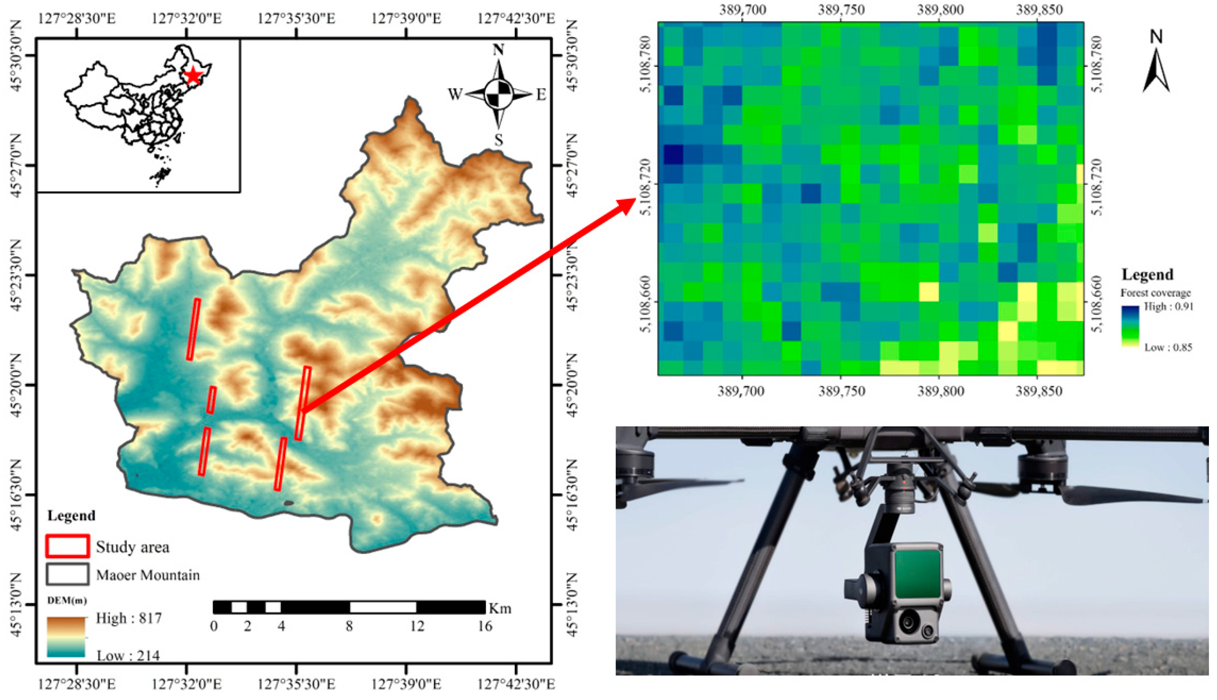
Maoer Mountain, with its complex terrain, was selected as the study area, which is located at 46°47′N and 127°28′E in Heilongjiang Province (Figure 1). The terrain gradually rises from south to north, with an average altitude of 300 m, and the highest peak is about 805 m. The region is located in a temperate monsoon climate with warm summers and cold winters. Affected by the climatic conditions, the forest coverage in this area is high, and the tree species are abundant, mainly including Pinus sylvestris, Pinus koraiensis, Larix olgensis, Fraxinus mandshurica, Juglans mandshurica, Ash, Walnut, and so on.
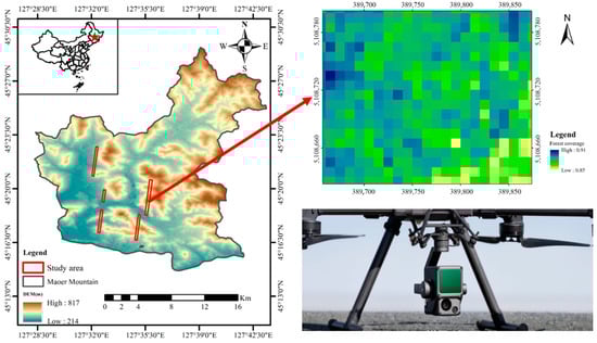
Figure 1.
The graph on the left represents the study area. The upper picture on the right shows the forest cover in the area shown and the lower figure shows the appearance of the drone sensor used in this experiment.
2.2. ATLAS Data
The altitude of the ICESat-2 orbit is about 500 km with an inclination angle and observation coverage of 92° and 88°S~88°N. The repetition period is 91 days, and each cycle has 1387 orbits. The ATLAS system is equipped with two lasers, typically only one in operation that emits a single pulse (532 nm) at a repetition rate of 10 kHz with a pulse width of 1.5 ns, which can acquire overlapping spots spaced approximately 0.7 m apart along the orbit and approximately 17 m in diameter. The ATLAS emits a total of 6 laser beams, arranged in 3 parallel groups along the orbit, each containing a strong signal and a weak signal, with an energy ratio of 4:1. The cross-orbit distance between each group is about 3.3 km, and the cross-orbit distance within the group is about 90 m. The flight trajectory of ICESat-2/ATLAS is shown in Figure 2.
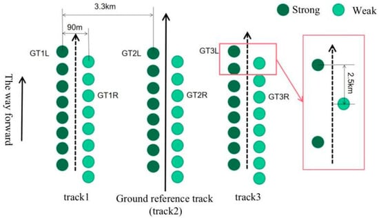
Figure 2.
Schematic diagram of the ICESat-2/ATLAS track.
2.3. Airborne Lidar Data
The drone lidar data were measured by DJI M300RTK equipped with DJI Zenmuse L1, and its RTK positioning accuracy was 1 cm ± 1 pm in the horizontal direction and 1.5 cm ± 1 pm in the vertical direction. The time interval between the collection of UAV lidar data and ATLAS data is one year, but this has little impact on the extraction of forest height in Maoer Mountain because there were no disturbances in this area during this period and the height of the upper forest remained almost unchanged. DTM and CHM are created using the following three steps: (1) The Improved Progressive TIN Densification (IPTD) [29] classification of ground points is first generated from seed points, and then layer-by-layer encryption is carried out through iterative processing until all ground points are classified. An irregular triangulation network (TIN) of ground points is then created and used to linearly interpolate DEM elevations into a 1 m raster grid. (2) Ground point normalization is used to remove the influence of terrain undulation on the elevation of point cloud data. (3) The CHM is created by selecting the maximum canopy height per 1 m grid cell and then interpolating it into a 1 m grating grid using the ground point cloud after normalization. DTM and CHM, with a resolution of 1 m, were used to verify the accuracy of the retrieved ground elevation and vegetation height from ATLAS data, respectively.
3. Methodology
3.1. Denoising
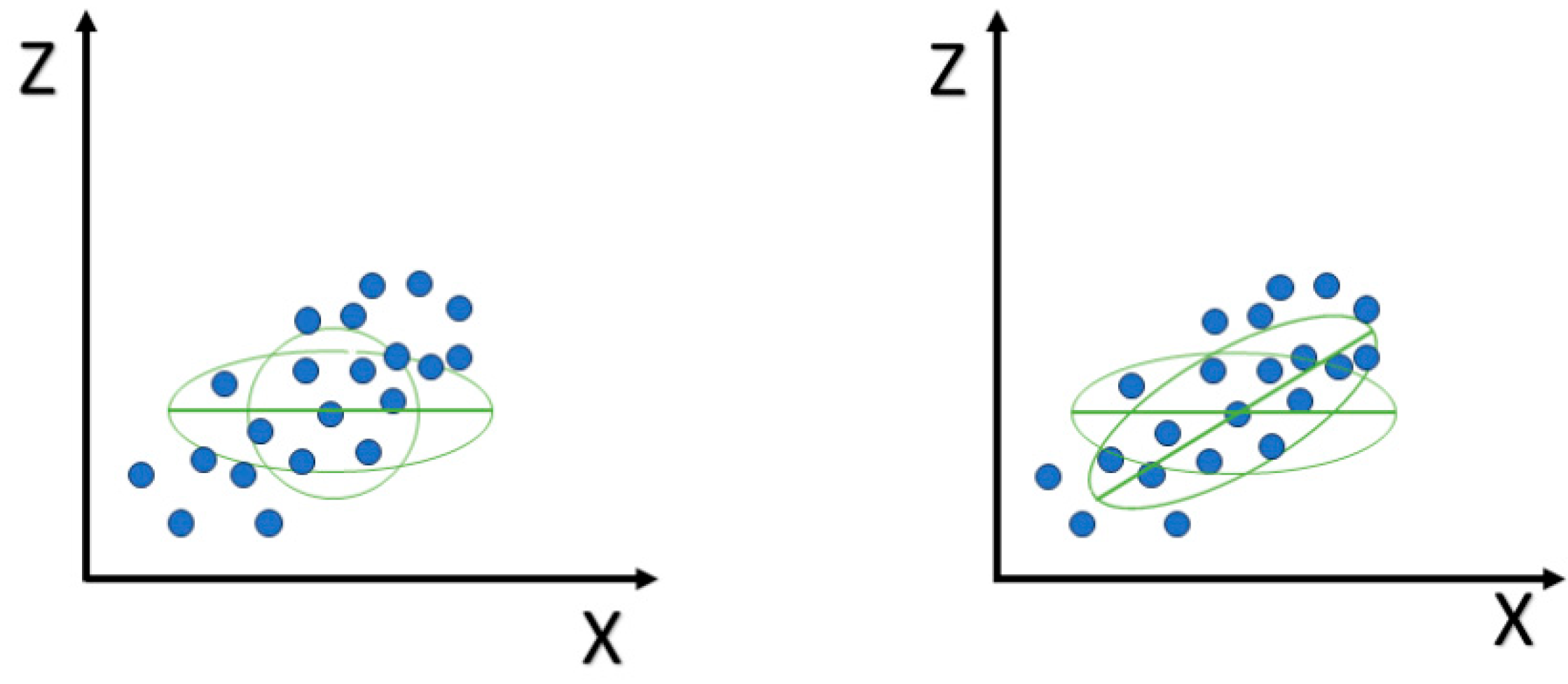
In order to reduce the increase in the amount of computation caused by excessive noise data, simple preliminary denoising of the point cloud data is carried out according to DEM, and only the photon point clouds within the range of 200 m above and below DEM are retained. In view of the obvious difference between the horizontal and vertical point cloud spacing, the density of signal photons is greater than that of noise photons. Therefore, the OPTICS algorithm [30], a density-based clustering analysis method, was used to denoise the photon point cloud. The OPTICS algorithm is an extension of the DBSCAN algorithm [31,32]. However, the DBSCAN algorithm depends on predefined parameters. Different predefined parameters will produce significantly different clustering results. The OPTICS algorithm requires the same input parameters of ε (the Neighborhood Radius) and MinPts (the Minimum Number of Neighborhood Points) as the DBSCAN algorithm. Unlike the DBSCAN algorithm, the OPTICS algorithm does not show the creation of a cluster. It generates cluster orderings and distance values for all photons to represent their density-based clustering structure. Due to the influence of the uneven distribution of photons in the horizontal and vertical directions, it is impossible to effectively distinguish between signal photon points and noise photon points; therefore, the circular search area in the OPTICS algorithm was improved to an elliptical search area in this study (Figure 3). Figure 3 shows the change in the search neighborhood from a circle to an ellipse and the change in the elliptical neighborhood after adjusting the direction.
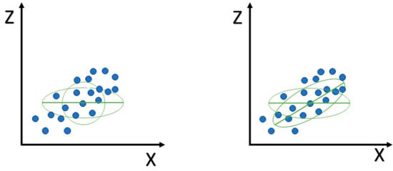
Figure 3.
Search for a neighborhood shape diagram. The circle and the ellipse represent the original neighborhood shape and the improved neighborhood shape, respectively.
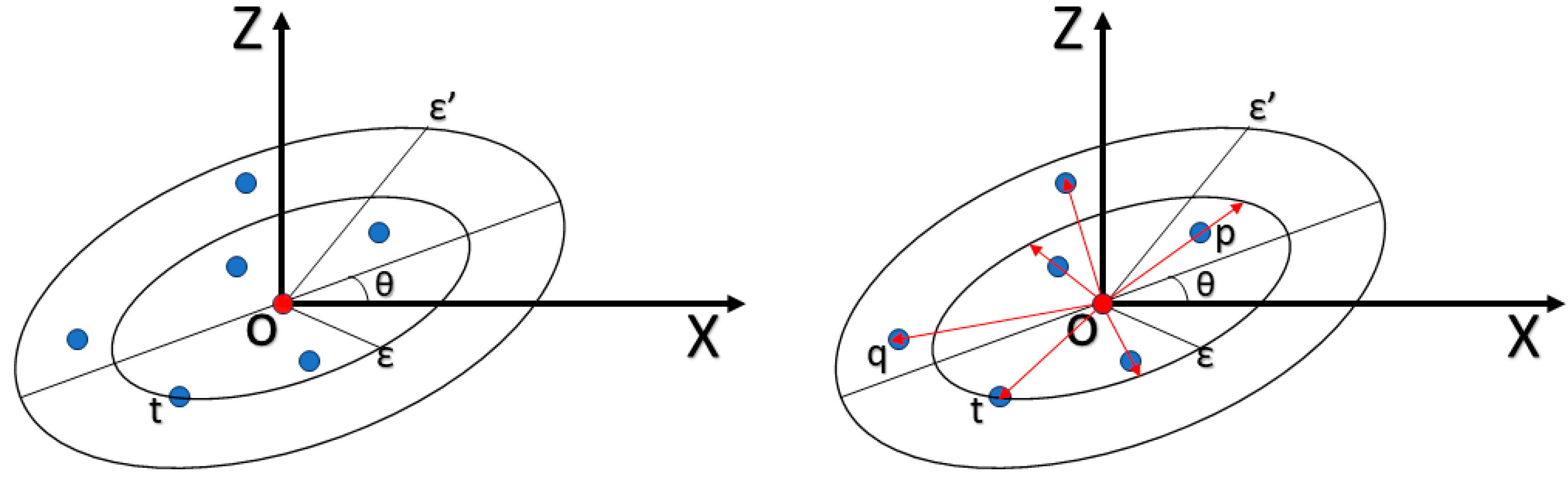
Usually, a horizontal ellipse neighborhood is not suitable for complex terrain because the point cloud signal in these areas will be seriously affected by the terrain slope. Therefore, it is necessary to adjust its angle so that its major semi-axis direction is parallel to the topographic direction to reduce the influence of topography (Figure 4). The algorithm considers that the direction in which the local photon points are densest is the same as the direction of the canopy and terrain inclination.
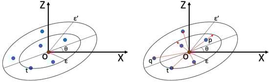
Figure 4.
Core distance and reachability distance schematic diagram. The red arrow indicates the distance from the center point to different locations. The circle and the ellipse represent the original neighborhood shape and the improved neighborhood shape, respectively.
The Core Distance (CD) (Equation (1)) and Reachability Distance (RD) (Equation (2)) of each sub-point were calculated according to the input parameters (ε and MinPts) of the improved OPTICS algorithm. ε and ε’ represent the number of photons in CD and RD, respectively.
where ε denotes the neighborhood radius, MinPts denotes the minimum number of photons in the ε neighborhood, Nε(o) denotes the number of photons in the ε neighborhood at the center point ‘o’, and represents the distance between the photon points q(xq, zq) and o(xo, zo) (where θ is the angle between the major semi-axis of the ellipse and the horizontal line).
Considering that some photon points correspond to multiple reachable distances, the minimum reachable distance of each photon is set as the optimal reachable distance. Finally, according to the characteristics of sparse noise photon distribution and dense signal photon distribution, the optimal reachable distance of all photon points and the OTSU (Nobuyuki Otsu) method are used to determine the threshold. The photon points were then divided into signal photons and noise photons with the calculated threshold (Equations (6)–(10)).
where P1 and P2 are the probabilities of being divided into the first and second categories, k is the hypothetical threshold, and m1 and m2 are the mean values of the two types of data, respectively. α2 is the between-class variance.
3.2. Photon Points Classification
3.2.1. Classification of Ground Points
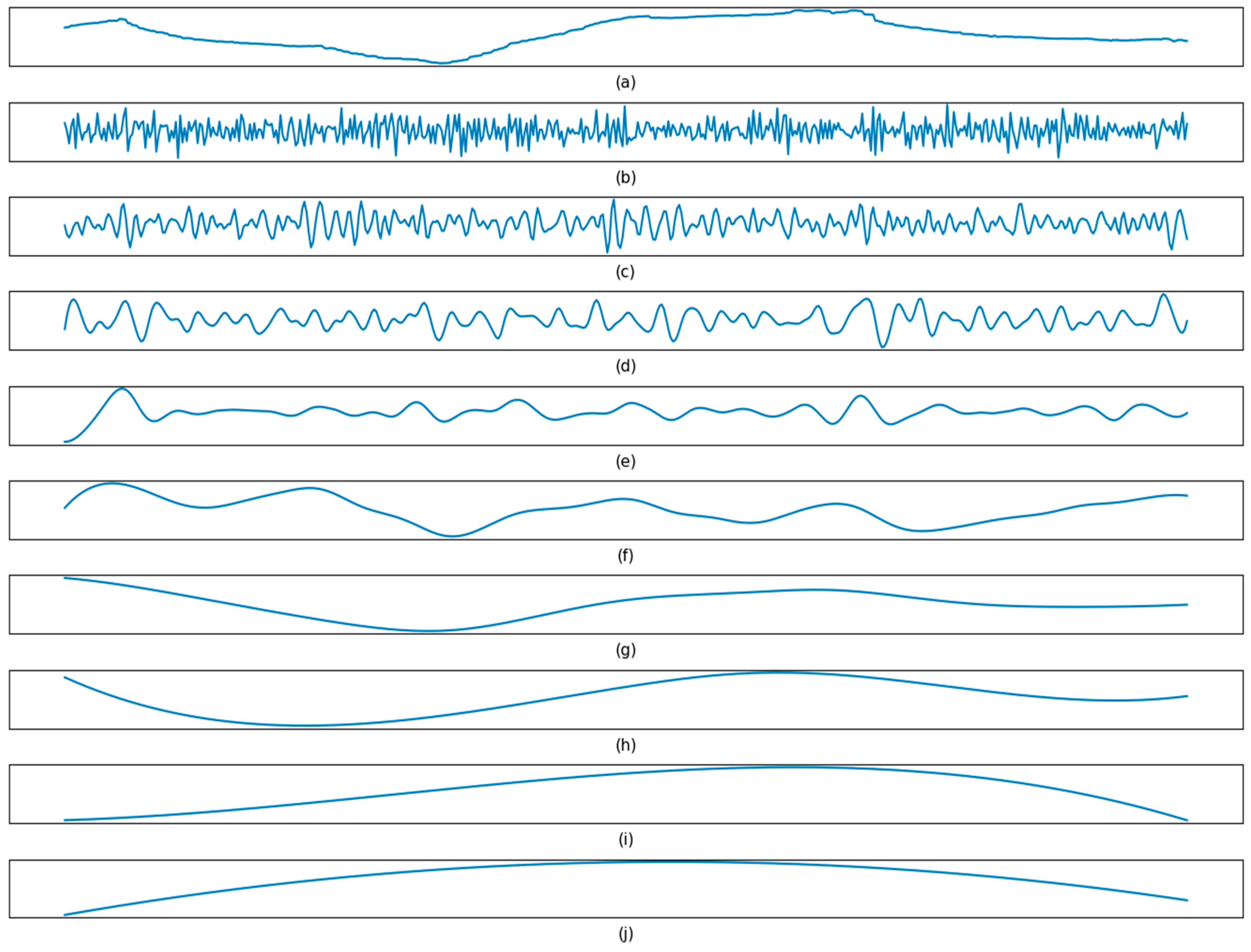
Compared with median filtering, the mean filter can use more photon points, which is conducive to generating smoother curves with higher accuracy. When vegetation covers the surface, the mean curve of the point cloud will be located between the forest canopy and the ground, and therefore photon points above the smoothing curve are identified as vegetation and those below are initially identified as the ground. The iterative mean calculation was used here three times to eliminate most of the vegetation points and retain the ground points, and finally, the continuous ground curve was smoothed by the filtering algorithm. However, there were still some noise points that deviated significantly from the ground curve. There were also some low-rise vegetation photons and near-ground plant-bottom photons incorrectly divided into ground photons, that is, pseudo-ground photons. In order to solve this problem, the EEMD (Ensemble Empirical Mode Decomposition) algorithm was used in this paper for the iterative removal of these discrete points. EEMD is a signal processing method improved from the idea of Empirical Mode Decomposition (EMD). EMD is a method of decomposing nonlinear and nonstationary signals into several Intrinsic Mode Functions (IMFs) (Figure 5), each of which satisfies the following two conditions: the number of local maxima and local minimum equals 1 or less than 1, and the average value of the IMF is 0 [33,34,35,36].
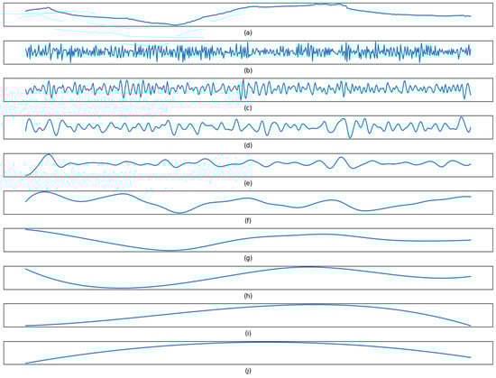
Figure 5.
The decomposition results of initial ground photons using EMD. (a) Original signal; (b) IMF 1; (c) IMF 2; (d) IMF 3; (e) IMF 4; (f) IMF 5; (g) IMF 6; (h) IMF 7; (i) IMF 8; (j) the final residual.
EEMD introduces basic noise analysis based on EMD, which effectively suppresses the modal aliasing effect of EMD and improves its application. First, white noise with a standard normal distribution was added to the original signal, the EDM decomposition was then performed to obtain the sums of all multiple IMFs, the process was repeated M times, and the amplitude of the white noise was different each time. Finally, using the principle that the statistical mean of the sequence is zero, the set average operation is performed on the IMF to obtain the final IMF of EEMD decomposition.
where x(t) is the original signal, ni(t) is white noise with a standard normal distribution (Equation (11)), xi(t) is the newly composed signal, ci,j(t) is the j-th IMF decomposed after adding the white noise for the i time, ri,j(t) is the residual function (Equation (12)), J is the number of IMFs, and xj(t) is the j-th IMF decomposed by EEMD (Equation (13)).
3.2.2. Classification of Canopy Points
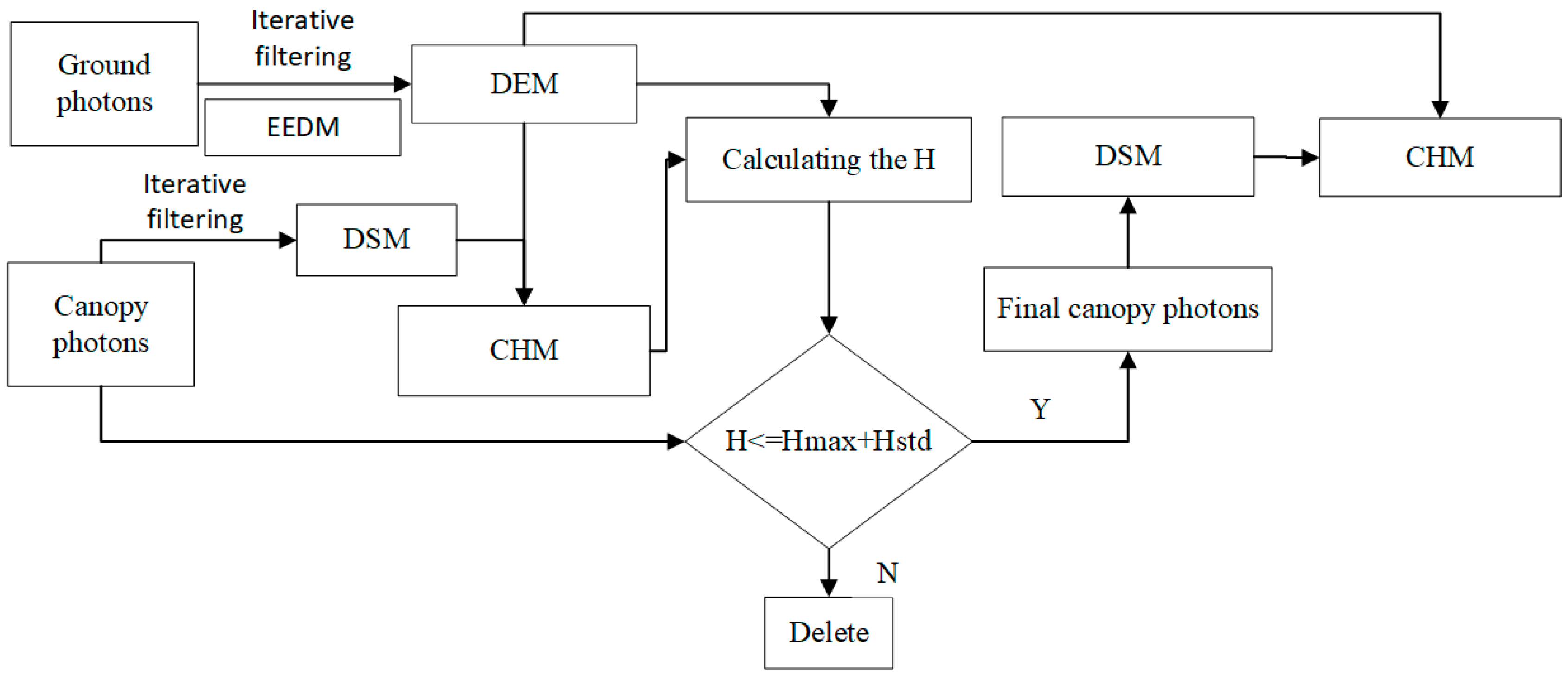
The forest canopy curve was obtained in a similar way as the ground curve. However, the ground curve tends to be more continuous and smoother with few abrupt changes. The canopy curve changes drastically in some areas due to forest gaps or forest disturbances. There is no vegetation cover on this part of the surface, therefore a window size of 20 m was chosen to calculate the height difference between the canopy and DEM. Values less than 2 m were considered to be an area without vegetation cover and the canopy height was set to 0. In addition, due to the poor continuity of the canopy, the direct smoothing of the canopy point cloud may cause a smooth transition after iterative mean filtering. Therefore, it is necessary to remove a portion of the false photons. First, the canopy photons need to be filtered iteratively to obtain the initial canopy curve; after that, the forest canopy height was calculated according to the ground and canopy curves. Then, the maximum and standard deviation of the forest canopy height were counted, respectively, and a small amount of the point cloud was removed by suitable threshold settings. Finally, the smooth canopy curve was obtained after the final canopy photon removal and interpolation (Figure 6).
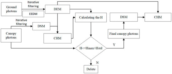
Figure 6.
Canopy photon recognition algorithm flow.
3.3. Estimation and Verification of Canopy Height
Canopy height was obtained at any location along the track direction as the elevation difference between the canopy curve and the ground curve. In this study, DTM and CHM with a resolution of 1 m × 1 m obtained from the airborne lidar data were used to assess the accuracy of ground elevation and canopy height, respectively. The performance of DSM, DEM, and forest canopy height under different slopes, vegetation coverage, and noise conditions will be evaluated by R2 and RMSE.
4. Results
4.1. Noise Removal
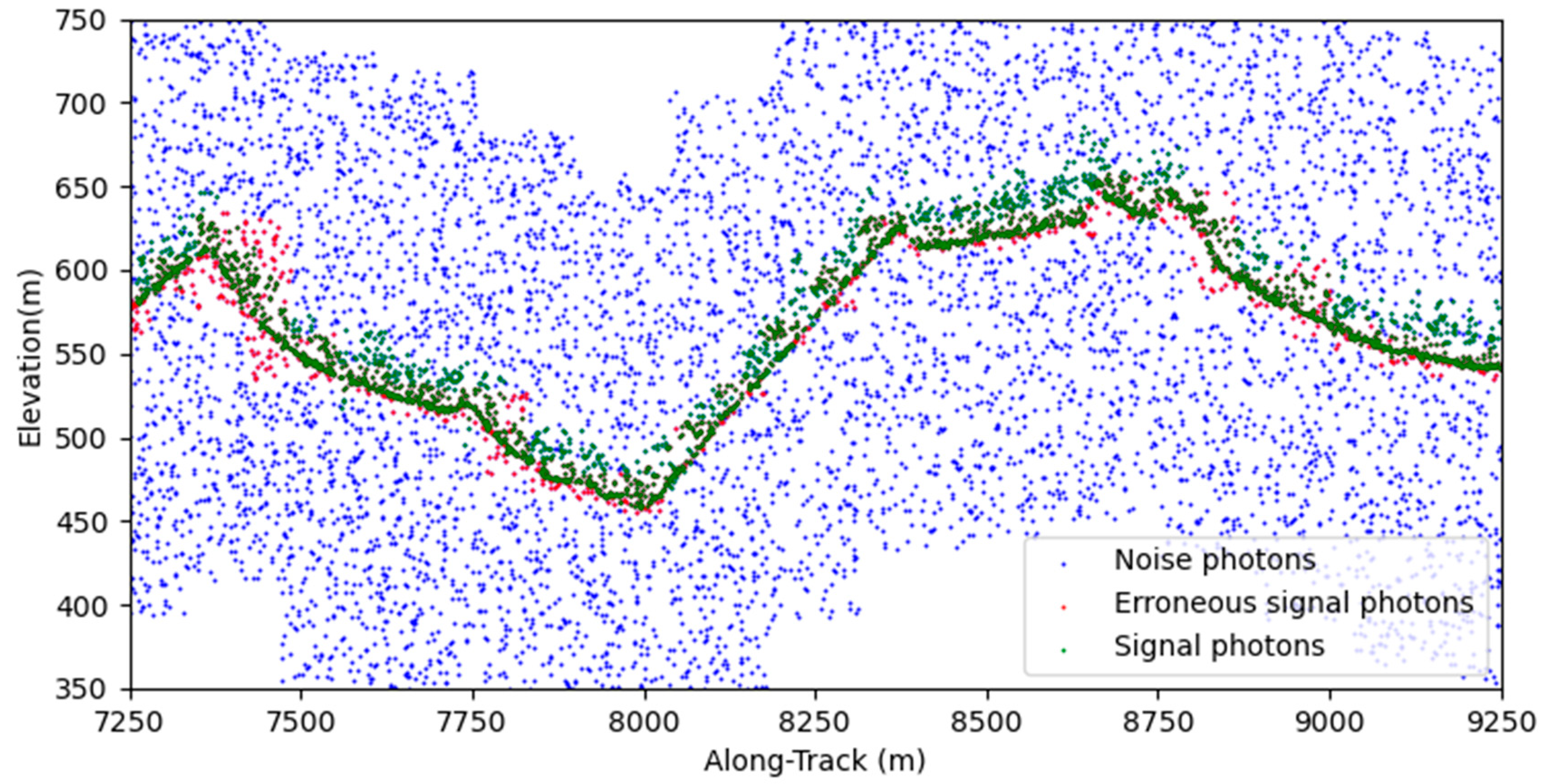
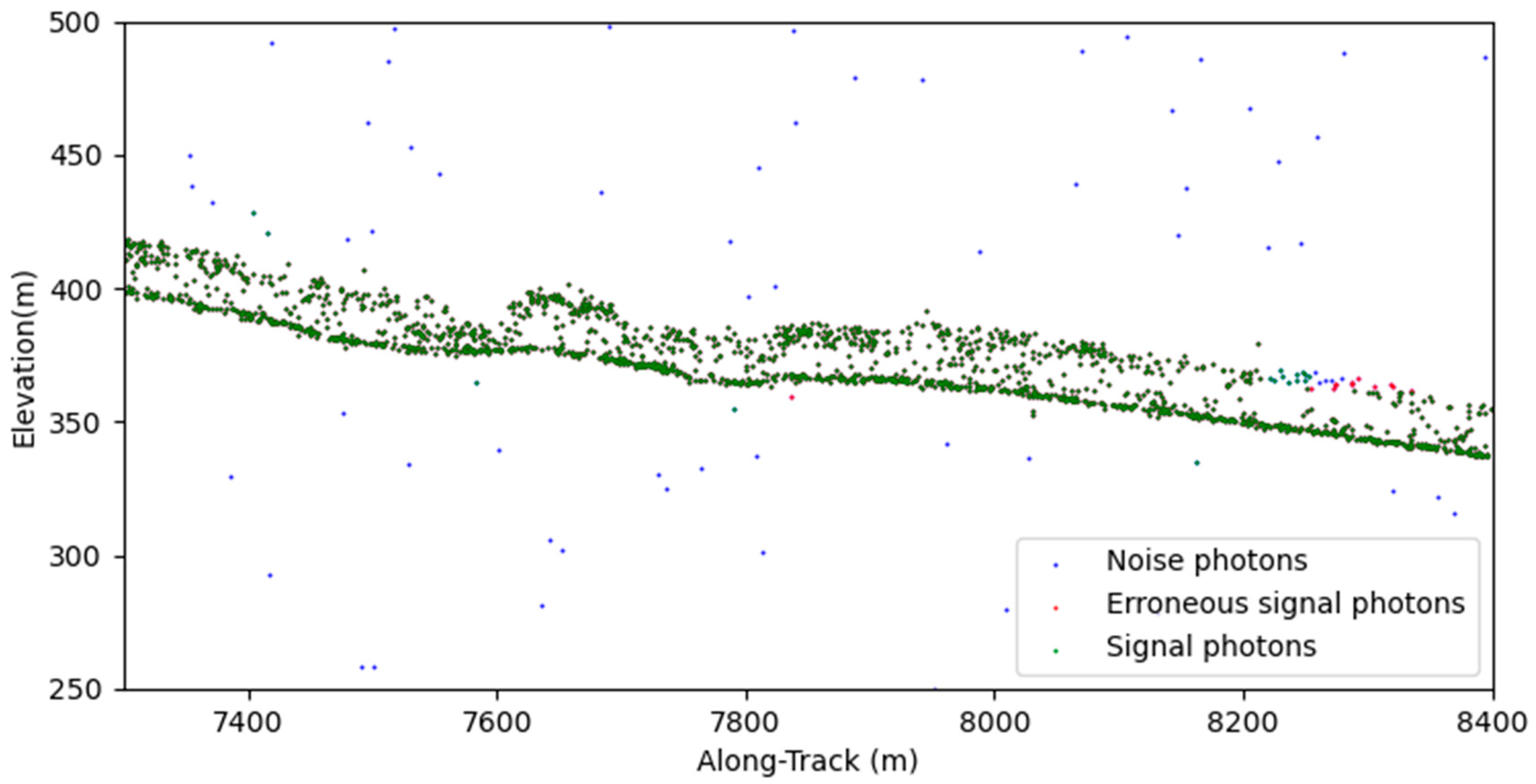
Using the algorithm developed in this study, signal photons can be reliably extracted from the original photons both at low signal-to-noise ratios (Figure 7) and high-signal-to-noise ratios (Figure 8). For denoising, the signal-to-noise ratio has a certain impact on the results of the algorithm, whereby the distance between the signal photons and the noise photons in the photon point cloud with a low signal-to-noise ratio will be closer and the density difference in the photon points will become smaller, which will become a major test for the denoising algorithm. By considering the directivity of the photons, the possible signal photons can be well preserved, especially in areas with steep terrain, as shown in Figure 8. Regardless of the slope of the terrain, the ground photons and canopy photons are completely preserved, and it is clear that the original algorithm of ATLAS can already control the noise but is not as good as the improved algorithm.
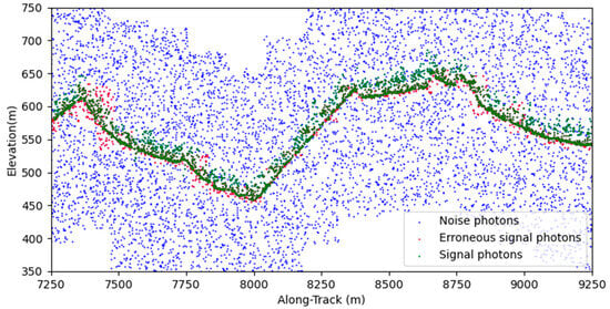
Figure 7.
The final results of noise-removal algorithm (low signal-to-noise ratio, complex terrain).
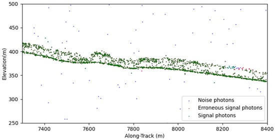
Figure 8.
The final results of noise-removal algorithm (high signal-to-noise ratio, relatively uncomplicated terrain).
Under the same signal-to-noise ratio, the improved algorithm outperforms the original algorithm in both types of terrain. In particular, the classification accuracy in hilly terrain significantly increased from 73.76% in the original method to 83.01%, which indicates a 9.25% improvement in correct classification (Table 1).

Table 1.
The performance of the two algorithms under different terrain conditions under the same signal-to-noise ratio.
Compared with different signal-to-noise ratio regions, the performance differences between the modified and original algorithms were small in the region with a low noise level; however, in the region with a low signal-to-noise ratio, the difficulty of distinguishing noise and signal increased, and the denoising effect of the proposed algorithm was better. The original algorithm will lose a large number of signal photons in the process of denoising, especially in areas with steep terrain and rapid terrain changes such as valleys and ridges, where the photon point cloud will produce discontinuity, resulting in no signal photons in this part of the area for the next step of photon point classification. This has a great impact on the subsequent calculations. This phenomenon is even more pronounced in the canopy, where many weak canopy photons are removed as noise photons because the continuity and density of photons in the canopy are not as good as those on the ground. This is also the case in areas where the slope of the terrain changes rapidly, and a significant reduction in effective signal photons can be clearly seen. It will have a large impact on the subsequent estimation of the canopy height, which will be underestimated due to the absence of some canopy photons. At the same time, it can be proved that when the distribution of the continuous points of the canopy and ground has an obvious trend in a certain direction, the shape and direction of their search neighborhoods should be modified to effectively improve the denoising results.
4.2. Photon Classification
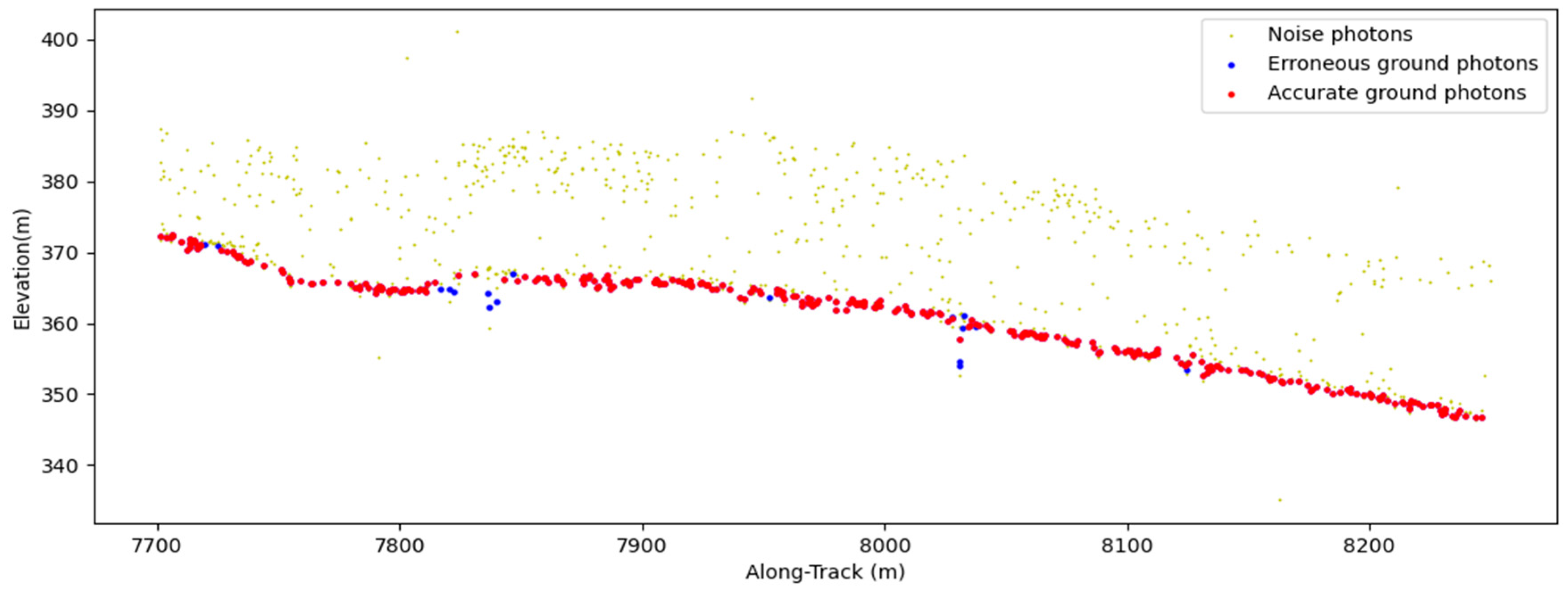
After noise removal in the first step, some of the noise points are still misclassified into terrestrial photons due to the close distance between the signal photons and the high photon density (Figure 9).

Figure 9.
The final ground photon extraction and the ground surface generation.
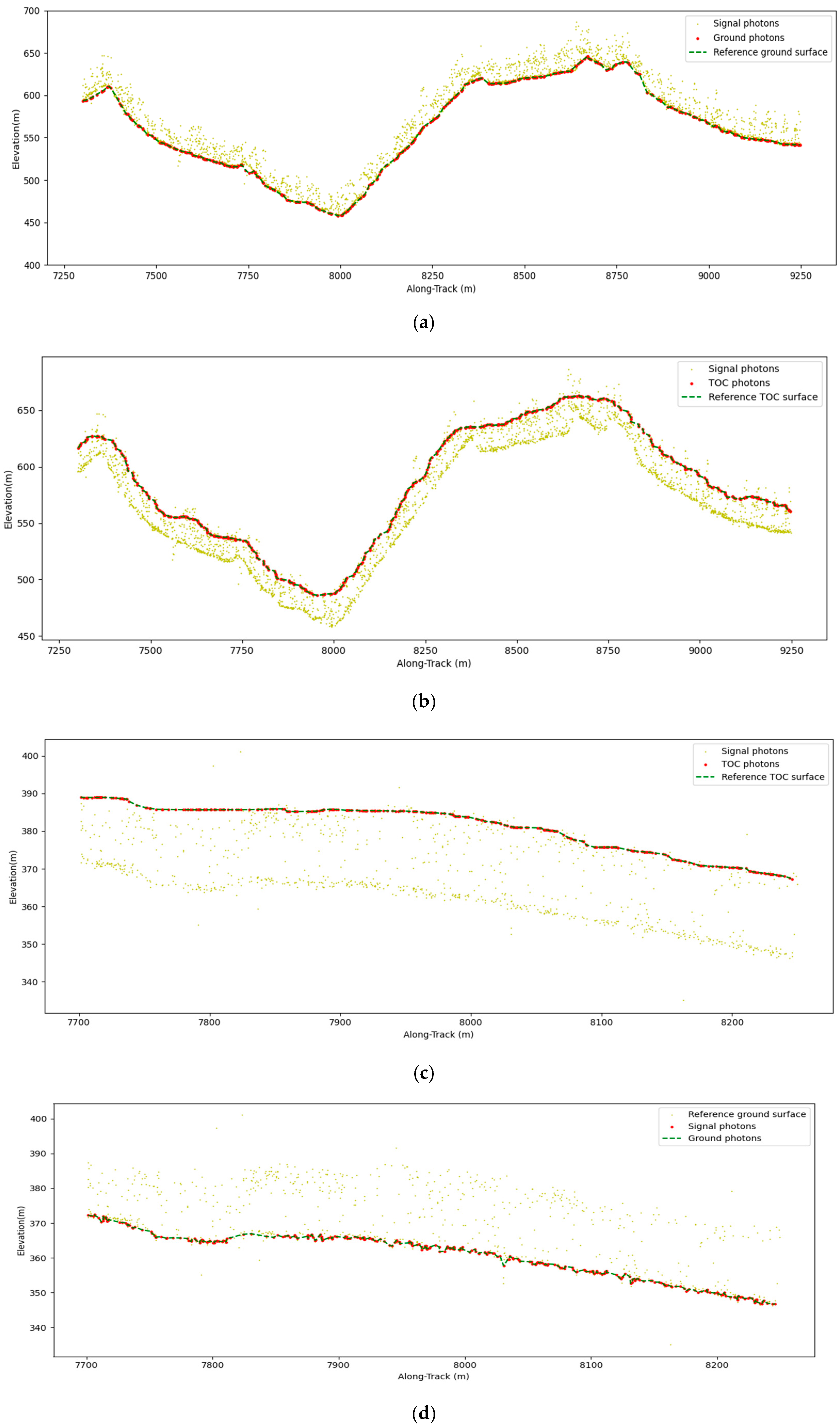
A qualitative analysis was conducted by comparing the processed canopy and ground surfaces and the reference DSM and DEM. The performance of the proposed algorithm under different noise conditions and different slope conditions is shown in Figure 10.
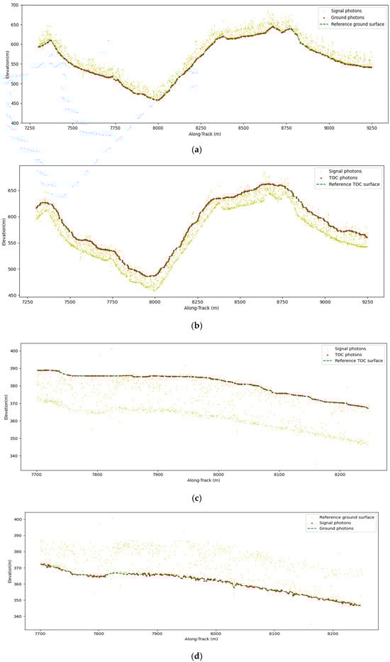
Figure 10.
(a–d) The DSM and DEM results for high signal-to-noise ratio and the DSM and DEM results for low signal-to-noise ratio, respectively.
In spaceborne lidar, a laser beam is emitted through a satellite and travels through the atmosphere. The slope may affect the propagation path and detection performance of the laser beam. On steep slopes, lidar may not be able to effectively cover all areas of the ground, resulting in incomplete detection data. The average slope of the navigation zone is 12.20° and the highest slope can reach 63.08°, so the terrain in this study area is complex. The accuracy of the improved optics algorithm for CHM detection was significantly higher than that before, with an improvement of 36.48%. However, RMSE still increased with the increase in slope, with an RMSE of 2.86 m in the relatively flat area and 4.97 m for the steep terrain. The average RMSE was 3.76 m, which was nearly 3 m lower than that of the original algorithm (Table 2). It can be seen that the modified algorithm has a better performance in DSM extraction. The main reason is that the original algorithm removed too many canopy points in the process of denoising, resulting in the loss of many canopy signal points.
Table 2.
The effect of slope on land surface extraction.
Compared to DSM, DEM was more accurate. The RMSE of the modified algorithm and the original algorithm was 1.19 m and 2.70 m, respectively. The accuracy of the original algorithm was greatly reduced in the area where the terrain changes rapidly due to the lack of signal photons, while for other areas, its accuracy was close to DEM obtained from the modified algorithm because of the higher continuity and lower uncertainty of the terrain than the canopy. The growth and natural succession of forests usually produce forest gaps, which lead to more uncertainty and discontinuity of the canopy.
The accuracy of CHM was slightly lower than both DEM and DSM. The RMSE of these two algorithms was 3.83 m and 6.03 m, respectively, which also gradually decreased with the continuous improvement of the slope. CHM decreased slightly in the area with higher coverage of vegetation because the canopy coverage also affects whether enough photons can reach the ground to obtain accurate ground curves. The R2 values of DEM, DSM, and CHM obtained by the two algorithms were all greater than 0.9, especially for the modified algorithm, which reached 0.99. The overall accuracy of the improved algorithm can reach 84.48%, of which the highest accuracy can exceed 85% when the slope is low and is close to 80% in areas with complex terrain and large slopes. Table 2 uses RMSE (Root Mean Square Error), R2 (R-Square), PA (Product Accuracy), and other indicators to evaluate the results.
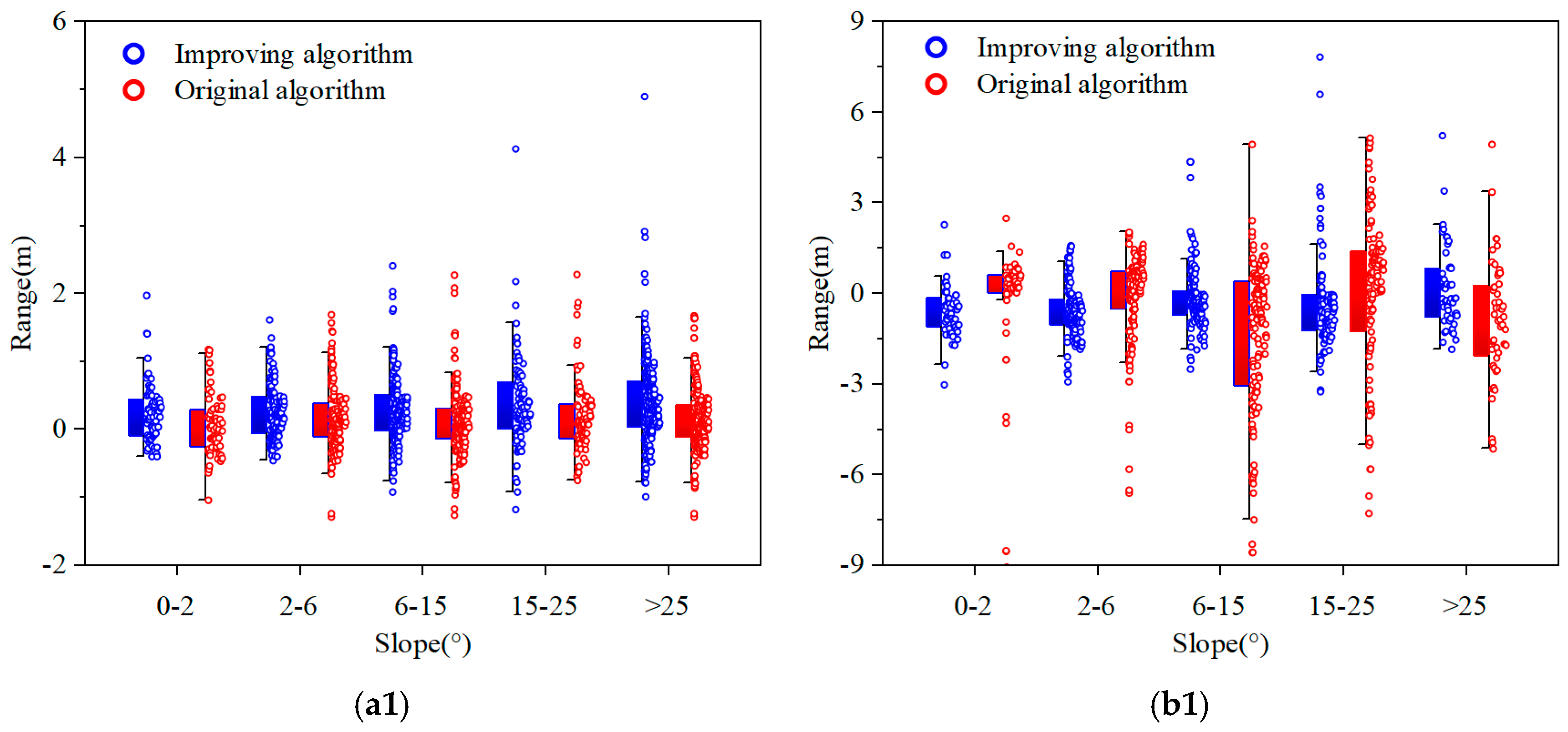
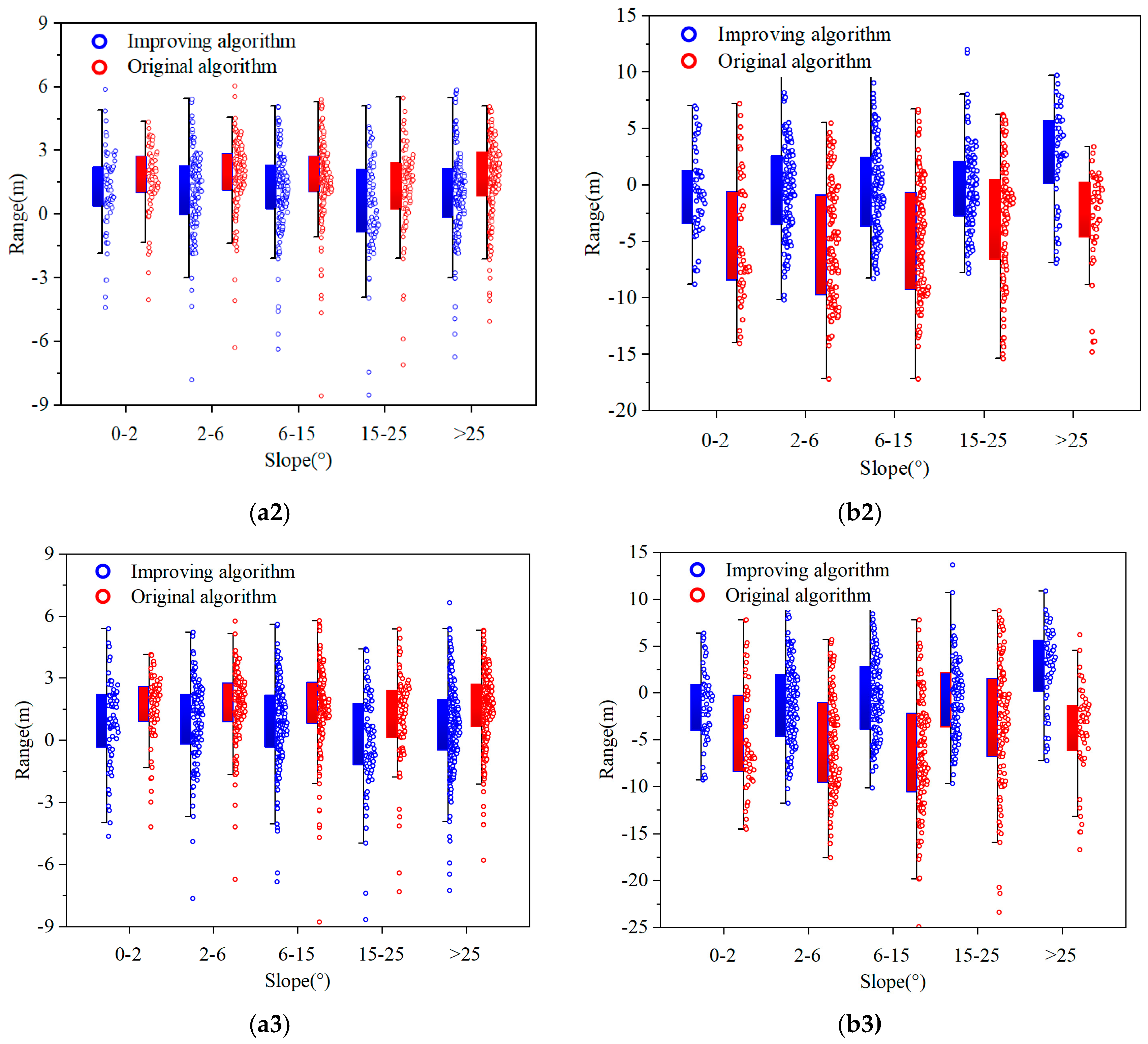
In general, it can be clearly seen that the accuracy of the modified algorithm was improved in the case of different slopes and signal-to-noise ratios, which was especially obvious in the case of more noise. The error fluctuation and outliers were all reduced and the results were more stable. Moreover, when the slope was large, the accuracy was significantly improved, which showed that the algorithm has good adaptability to the slope and can significantly reduce the error caused by the slope (Figure 11).

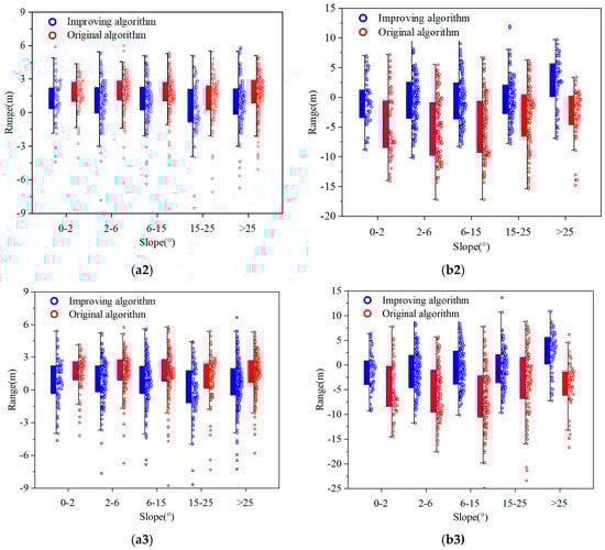
Figure 11.
(a1–a3) The DEM, DSM, and CHM error box plots in the high signal-to-noise ratio region and (b1–b3) the DEM, DSM, and CHM error box plots in the low signal-to-noise ratio region, respectively. I stands for improved algorithm and O stands for original algorithm.
The forest canopy height calculated in this paper was mainly for the area with vegetation coverage of less than 0.2, ignoring the area with vegetation coverage of less than 0.2. Vegetation coverage affects whether the photons can reach the ground through the dense canopy to a certain extent. Too low coverage will result in the failure of DSM extraction.
The accuracy of the algorithm is more than 80%, which is higher than that of the original algorithm under any forest cover, and it can accurately estimate the ground elevation and forest canopy height (Table 3). The highest accuracy of the original algorithm and the improved algorithm in estimating canopy height appeared in the area with a forest coverage rate of 0.4–0.6 and 0.6–0.8 and RMSE of 4.74 and 3.36, respectively, indicating that the improved algorithm has a good estimation ability for high vegetation coverage and the impact of vegetation coverage is far less than that of the original algorithm. Compared with the original algorithm, the algorithm improved by 20% to 40% in RMSE and about 10% in product accuracy. The accuracy of DEM estimation by the original algorithm decreased with the increase in vegetation coverage, while the accuracy of DEM estimation was influenced by vegetation coverage, with the improved algorithm greatly reduced and relatively stable. The results for DEM retrieval with high accuracy can be obtained in different vegetation coverage regions. In general, among the different influencing factors, the influence of slope is greater, and the impact of forest cover will also have a certain impact, but the impact is relatively as small as that of slope. For the area with a high signal-to-noise ratio, there is little difference between the accuracy results of the two, and the variation in accuracy with vegetation coverage is similar to that in the case of a low signal-to-noise ratio. This indicates that for the study of forest canopy extraction using ATLAS data, the signal-to-noise ratio does not change the influence of the algorithm on other factors. The signal photons can be more effectively distinguished in the area with low noise, and more signal photons play an important role in the later process of point cloud classification and canopy height estimation. In the case of a low signal-to-noise ratio, low vegetation coverage may lead to a further reduction in canopy photon points and photon density, making the difference between the canopy photons smaller and more difficult to separate. There may be a possibility that the signal photons are removed as noise photons in the denoising process, and the reduction in canopy photons will inevitably lead to a reduction in DSM accuracy. This can also occur in the case of high signal-to-noise ratios but its impact is smaller. More noise can lead to a decrease in the accuracy of the canopy height in the area. However, due to the penetration of lidar and the obstruction of vegetation, the impact of noise on ground points is small.
Table 3.
The effect of vegetation cover on land surface extraction.
It can be seen in Table 4 that the type of forest stand also has an impact on the accuracy of the algorithm. For coniferous forests, DEM provides the lowest RMSE (0.95 m), indicating that DEM has higher accuracy in canopy height extraction in coniferous forests. In contrast, the RMSE values for DSM (3.05 m) and CHM (2.89 m) are larger. For broadleaf forests, DEM also has the lowest RMSE (1.28 m), compared to DSM (3.49 m) and CHM (3.45 m), indicating that DEM performs better in terms of prediction accuracy in broadleaf forests as well.
Table 4.
Effect of stand type on forest canopy height extraction.
The results presented in Table 4 indicate that the Digital Elevation Model (DEM) yields the best performance across both forest types, particularly in coniferous forests, where it exhibits lower RMSE and higher PA. Although both the Digital Surface Model (DSM) and the Canopy Height Model (CHM) demonstrate very high R2 values (close to 1), their accuracy and consistency are notably reduced in broadleaf forests. This disparity suggests that forest type (coniferous vs. broadleaf) plays a significant role in influencing the performance of these data types. Such variations may be attributed to differences in forest structure and canopy characteristics between the two forest types.
5. Discussion
5.1. Effect of Slope
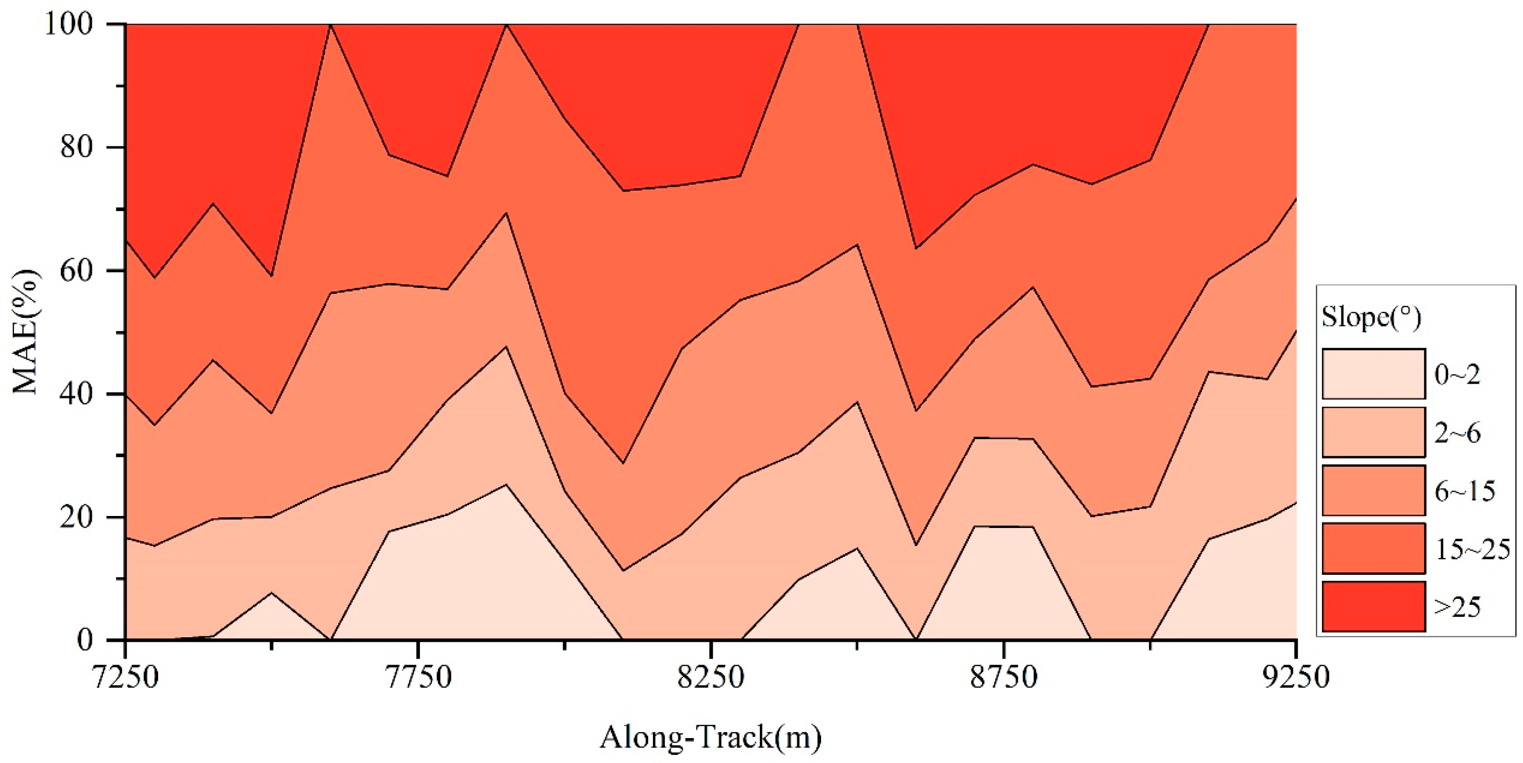
An improved algorithm was proposed in this study to accurately retrieve ground elevation and vegetation height from photon-counting lidar data. It introduced a noise-removal algorithm based on local statistics that improves photon classification. It can be seen from the results of this paper that each denoising and photon classification algorithm will be affected by the signal-to-noise ratio of the original data. The more noise photons, the more difficult it is to distinguish between noise and signal photons, thereby reducing the accuracy of subsequent parameter calculations. The slope has a very important impact on the extraction of ground elevation, surface elevation, and forest canopy height [29,37]. The accuracy of these three items will gradually decrease with the increase in slope. The accuracy of canopy height retrieval was lower in the mountainous area with complex terrain changes. The influence of slope was not only the value of the slope itself but also its change rate, that is, the complexity of the terrain. In addition to improving the accuracy of the estimation of forest canopy height, the algorithm can also improve the stability of the results, and it can be seen that after the improvement of the algorithm, the RMSE range of the accuracy results is smaller and more concentrated and the results are more stable (Figure 12).
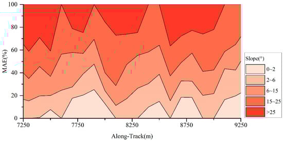
Figure 12.
Scatter plot of the change in the orbital direction of the residual extension satellite due to slope.
5.2. Effect of Forest Cover
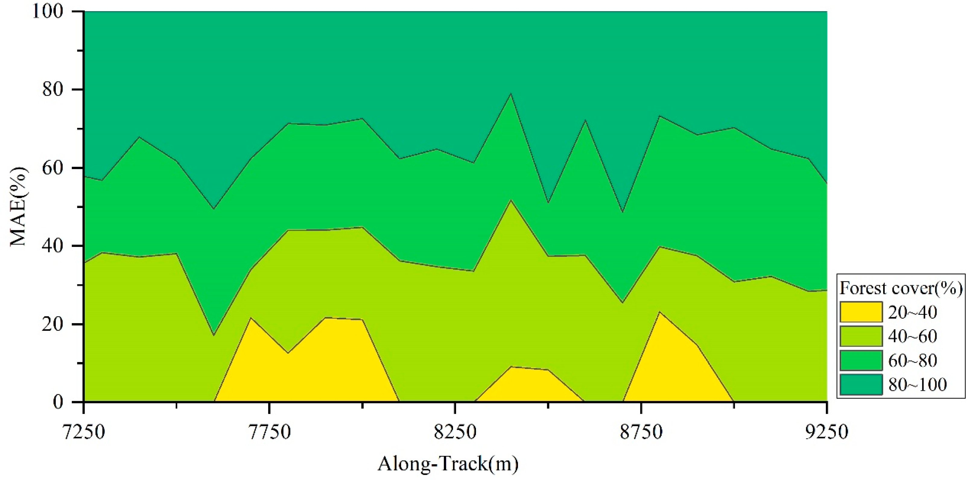
Vegetation coverage was also one of the influencing factors affecting the accuracy of the canopy extraction algorithm, whereby the lower the coverage, the higher the accuracy of DEM [38,39]. Canopy and ground photons are easy to confuse in high vegetation coverage, which may slightly reduce the accuracy of canopy height estimation. Vegetation coverage has a significant impact on lidar. Lidar obtains information about the surface and vegetation by emitting a laser beam and measuring its echo signal. Vegetation coverage is also one of the factors that have a great impact on the penetration of the laser, and when the laser beam propagates above the vegetation, it will reflect and scatter with the vegetation leaves, branches, and other structures. These scattered signals can interfere with the echo signal of the original laser beam, weakening or distorting the received signal of the lidar, resulting in degraded data quality. As a result, dense vegetation increases the scattered signal received by the sensor, making the echo signal intense and complex to parse. The effect of multiple reflections on laser mines is that they increase their propagation path and time. When a laser mine passes over a reflective surface, it can undergo multiple reflections, causing the light rays to travel in different directions. This causes the energy of the laser mine to be dispersed and weakened. In addition, multiple reflections may also cause scattering and interference of the beam, which affects the focus and accuracy of the laser mine. The vegetation coverage affects the penetration ability of lidar. Dense layers of vegetation prevent laser beams from reaching the surface directly. This makes it impossible for lidar to obtain information about the underlying layers of the land, limiting the accuracy of topographic surveys and geomorphological analysis (Figure 13).

Figure 13.
Scatter plot of orbital direction change in residual extension satellite affected by forest cover.
Upon further investigation into the impact of slope and forest coverage on the improvement of the algorithm, both had a significant effect on the accuracy of the algorithm, with a similar degree of influence. Specifically, the impact of forest coverage was slightly greater, accounting for approximately 53%, while slope accounted for 47%.
5.3. Other Effects
The observation time also has an important impact on the accuracy of canopy height estimation. The number of noise photons obtained at night is significantly less than that of the daytime data, with a high signal-to-noise ratio. This is mainly due to the increase in noise, as the difficulty of effective separation will increase. Too much noise will weaken the density characteristics of the effective signal so that the two are more similar and difficult to distinguish. The accuracy of the effective signal is the premise of the subsequent acquisition of forest canopy height.
Stand type also has an important impact on the accuracy of canopy height estimation. It is estimated that the RMSE of coniferous forests is about 10%, higher than that of broadleaf forests. Due to the different composition of the tree species in different stands, with different leaf shapes and canopy structures, the interforest signal photons in the coniferous forest are more abundant and the signal-to-noise ratio is higher. The probability of photons passing through the coniferous is increased, while the blocking of the wide leaf makes it more difficult to obtain effective photons, making noise and signals more similar and indistinguishable and pseudo-ground and real ground points more likely to be confused. The accuracy of the valid signal is a prerequisite for obtaining the height of the forest canopy in the future, and the above situation reduces its accuracy. Therefore, the estimation result in coniferous forests will be better than that of broad-leaved forests.
6. Conclusions
In this study, an improved OPTICS algorithm was developed to remove the noise points of the ATLAS data, and then the processing method was changed according to the characteristics of photons and ground photons in the vegetation canopy to obtain the correct signal photons. The DEM and DSM were further extracted by filtering, and finally, the forest canopy height was obtained. This paper analyzes the influence of the improved algorithm on extraction accuracy due to factors such as forest coverage, slope, and vegetation type. Compared with the original algorithm, the adaptability of the improved algorithm to the above effects is also discussed. Based on the verification of ground elevation and canopy height, the conclusions in this study were as follows: (1) the noise-removal algorithm proposed in this study can reduce the influence of photon directionality caused by slope factors and effectively remove noise photons while retaining more effective signal photons; and (2) the improved filtering algorithm can make more effective use of signal photons, improve the accuracy of extracting ground photons and canopy photons, and thus improve the accuracy of DEM, DSM, and CHM. The new proposed algorithm can provide a valuable basis for estimating ground elevation and vegetation height. However, in densely vegetated areas, the emitted pulses may not penetrate the vegetation canopy and reach the surface, which makes noise removal and photon classification difficult and subsequently limits the estimation accuracy of ground elevation and vegetation height. When calculating the DEM, the vegetation near the ground may be considered as ground points, resulting in the absence of some ground points, which can be improved. In addition, ICESat-2 data can be combined with other data, such as optical images, airborne lidar, radar, and GEDI data, to take advantage of their different measurement methods and characteristics and expand their potential applications.
Author Contributions
Conceptualization, G.W. and Y.Y.; methodology, G.W.; writing—original draft preparation, G.W.; writing—review and editing, M.L., X.Y., and Y.Y.; software, H.D. and X.G. All authors have read and agreed to the published version of the manuscript.
Funding
This research was funded by the National Natural Science Foundation of China (grant number 32471855) and the Fundamental Research Funds for the National Key Research and Development Program of China (grant number 2023YFD2201704).
Data Availability Statement
The raw data supporting the conclusions of this article will be made available by the authors on request.
Conflicts of Interest
The authors declare no conflicts of interest.
References
- Zhang, G.; Ganguly, S.; Nemani, R.R.; White, M.A.; Milesi, C.; Hashimoto, H.; Wang, W.; Saatchi, S.; Yu, Y.; Myneni, R.B. Estimation of Forest Aboveground Biomass in California Using Canopy Height and Leaf Area Index Estimated from Satellite Data. Remote Sens. Environ. 2014, 151, 44–56. [Google Scholar] [CrossRef]
- Chen, Q. Retrieving Vegetation Height of Forests and Woodlands over Mountainous Areas in the Pacific Coast Region Using Satellite Laser Altimetry. Remote Sens. Environ. 2010, 114, 1610–1627. [Google Scholar] [CrossRef]
- Kelly, M.; Su, Y.; Di Tommaso, S.; Fry, D.; Collins, B.; Stephens, S.; Guo, Q. Impact of Error in Lidar-Derived Canopy Height and Canopy Base Height on Modeled Wildfire Behavior in the Sierra Nevada, California, USA. Remote Sens. 2017, 10, 10. [Google Scholar] [CrossRef]
- Sačkov, I.; Kardoš, M. Forest Delineation Based on LiDAR Data and Vertical Accuracy of the Terrain Model in Forest and Non-Forest Area. Ann. For. Res. 2014, 57, 119–136. [Google Scholar] [CrossRef]
- Zhang, W.; Liu, Y.; Shen, M.; Chen, X.; Chen, R. Spatiotemporal Variation of Net Primary Productivity and Response to Climatic Factors in the Yangtze River Basin. Water Resour. Hydropower Eng. 2022, 53, 165–176. [Google Scholar] [CrossRef]
- Zhou, J.; Zhang, K.; Du, T. Research of Vegetation Cover Variations in Reservoir Areas Based on Satellite Remote Sensing: A Case Study of Sanhekou Reservoir Area. Water Resour. Hydropower Eng. 2024, 55, 134–147. [Google Scholar] [CrossRef]
- Li, Y.; Shang, R.; Qu, Y. Assessment of the Dynamics of Vegetation Net Primary Productivity and Its Response to Environmental Chan-Ges before and after the Grain for Green Project: A Case Study Form the Loess Plateau of Northern Shaanxi. Water Resour. Hydropower Eng. 2023, 54, 156–166. [Google Scholar] [CrossRef]
- Potapov, P.; Li, X.; Hernandez-Serna, A.; Tyukavina, A.; Hansen, M.C.; Kommareddy, A.; Pickens, A.; Turubanova, S.; Tang, H.; Silva, C.E.; et al. Mapping Global Forest Canopy Height through Integration of GEDI and Landsat Data. Remote Sens. Environ. 2021, 253, 112165. [Google Scholar] [CrossRef]
- Fu, H.; Zhu, J.; Wang, C.; Wang, H.; Zhao, R. Underlying Topography Estimation over Forest Areas Using High-Resolution P-Band Single-Baseline PolInSAR Data. Remote Sens. 2017, 9, 363. [Google Scholar] [CrossRef]
- Niemi, M.; Vauhkonen, J. Extracting Canopy Surface Texture from Airborne Laser Scanning Data for the Supervised and Unsupervised Prediction of Area-Based Forest Characteristics. Remote Sens. 2016, 8, 582. [Google Scholar] [CrossRef]
- Parker, G.G.; Russ, M.E. The Canopy Surface and Stand Development: Assessing Forest Canopy Structure and Complexity with near-Surface Altimetry. For. Ecol. Manag. 2004, 189, 307–315. [Google Scholar] [CrossRef]
- González-Jaramillo, V.; Fries, A.; Zeilinger, J.; Homeier, J.; Paladines-Benitez, J.; Bendix, J. Estimation of Above Ground Biomass in a Tropical Mountain Forest in Southern Ecuador Using Airborne LiDAR Data. Remote Sens. 2018, 10, 660. [Google Scholar] [CrossRef]
- Nie, S.; Wang, C.; Zeng, H.; Xi, X.; Xia, S. A Revised Terrain Correction Method for Forest Canopy Height Estimation Using ICESat/GLAS Data. ISPRS J. Photogramm. Remote Sens. 2015, 108, 183–190. [Google Scholar] [CrossRef]
- Qin, H.; Wang, C.; Xi, X.; Tian, J.; Zhou, G. Estimation of Coniferous Forest Aboveground Biomass with Aggregated Airborne Small-Footprint LiDAR Full-Waveforms. Opt. Express 2017, 25, A851. [Google Scholar] [CrossRef]
- Yamamoto, K.H.; Powell, R.L.; Anderson, S.; Sutton, P.C. Using LiDAR to Quantify Topographic and Bathymetric Details for Sea Turtle Nesting Beaches in Florida. Remote Sens. Environ. 2012, 125, 125–133. [Google Scholar] [CrossRef]
- Ballhorn, U.; Jubanski, J.; Siegert, F. ICESat/GLAS Data as a Measurement Tool for Peatland Topography and Peat Swamp Forest Biomass in Kalimantan, Indonesia. Remote Sens. 2011, 3, 1957–1982. [Google Scholar] [CrossRef]
- Jang, J.-D.; Payan, V.; Viau, A.A.; Devost, A. The Use of Airborne Lidar for Orchard Tree Inventory. Int. J. Remote Sens. 2008, 29, 1767–1780. [Google Scholar] [CrossRef]
- Mahoney, C.; Hopkinson, C.; Kljun, N.; Van Gorsel, E. Estimating Canopy Gap Fraction Using ICESat GLAS within Australian Forest Ecosystems. Remote Sens. 2017, 9, 59. [Google Scholar] [CrossRef]
- Murgoitio, J.; Shrestha, R.; Glenn, N.; Spaete, L. Airborne LiDAR and Terrestrial Laser Scanning Derived Vegetation Obstruction Factors for Visibility Models. Trans. GIS 2014, 18, 147–160. [Google Scholar] [CrossRef]
- Pourrahmati, M.R.; Baghdadi, N.N.; Darvishsefat, A.A.; Namiranian, M.; Fayad, I.; Bailly, J.-S.; Gond, V. Capability of GLAS/ICESat Data to Estimate Forest Canopy Height and Volume in Mountainous Forests of Iran. IEEE J. Sel. Top. Appl. Earth Obs. Remote Sens. 2015, 8, 5246–5261. [Google Scholar] [CrossRef]
- Magruder, L.; Neumann, T.; Kurtz, N. The Ice, Cloud and Land Elevation Satellite-2 (ICESat-2): Mission Status, Science Results and Outlook. 2021. Available online: https://ui.adsabs.harvard.edu/abs/2021EGUGA..23.8967M/abstract (accessed on 20 November 2024).
- Herzfeld, U.C.; Trantow, T.M.; Harding, D.; Dabney, P.W. Surface-Height Determination of Crevassed Glaciers—Mathematical Principles of an Autoadaptive Density-Dimension Algorithm and Validation Using ICESat-2 Simulator (SIMPL) Data. IEEE Trans. Geosci. Remote Sens. 2017, 55, 1874–1896. [Google Scholar] [CrossRef]
- Zhang, J.; Kerekes, J. An Adaptive Density-Based Model for Extracting Surface Returns From Photon-Counting Laser Altimeter Data. IEEE Geosci. Remote Sens. Lett. 2015, 12, 726–730. [Google Scholar] [CrossRef]
- Febriana, N.L.; Sitanggang, I.S. Outlier Detection on Hotspot Data in Riau Province Using OPTICS Algorithm. IOP Conf. Ser. Earth Environ. Sci. 2017, 58, 012004. [Google Scholar] [CrossRef]
- Pan, J.; Gao, F.; Wang, J.; Zhang, J.; Liu, Q.; Deng, Y. A Main Direction-Based Noise Removal Algorithm for ICESat-2 Photon-Counting LiDAR Data. J. Geod. 2024, 98, 80. [Google Scholar] [CrossRef]
- Popescu, S.C.; Zhou, T.; Nelson, R.; Neuenschwander, A.; Sheridan, R.; Narine, L.; Walsh, K.M. Photon Counting LiDAR: An Adaptive Ground and Canopy Height Retrieval Algorithm for ICESat-2 Data. Remote Sens. Environ. 2018, 208, 154–170. [Google Scholar] [CrossRef]
- Yang, X.; Wang, C.; Nie, S.; Xi, X.; Hu, Z.; Qin, H. Application and Validation of a Model for Terrain Slope Estimation Using Space-Borne LiDAR Waveform Data. Remote Sens. 2018, 10, 1691. [Google Scholar] [CrossRef]
- Chen, B.; Pang, Y.; Li, Z.; Lu, H.; Liu, L.; North, P.R.J.; Rosette, J.A.B. Ground and Top of Canopy Extraction From Photon-Counting LiDAR Data Using Local Outlier Factor With Ellipse Searching Area. IEEE Geosci. Remote Sens. Lett. 2019, 16, 1447–1451. [Google Scholar] [CrossRef]
- Zhao, X.; Guo, Q.; Su, Y.; Xue, B. Improved Progressive TIN Densification Filtering Algorithm for Airborne LiDAR Data in Forested Areas. ISPRS J. Photogramm. Remote Sens. 2016, 117, 79–91. [Google Scholar] [CrossRef]
- Guo, Y.; Zhong, L.; Min, L.; Wang, J.; Wu, Y.; Chen, K.; Wei, K.; Rao, C. Adaptive Optics Based on Machine Learning: A Review. Opto-Electron. Adv. 2022, 5, 200082. [Google Scholar] [CrossRef]
- Schubert, E.; Sander, J.; Ester, M.; Kriegel, H.P.; Xu, X. DBSCAN Revisited, Revisited. ACM Trans. Database Syst. 2017, 42, 1–21. [Google Scholar] [CrossRef]
- Hahsler, M.; Piekenbrock, M.; Doran, D. Dbscan: Fast Density-Based Clustering with R. J. Stat. Softw. 2019, 91, 1–30. [Google Scholar] [CrossRef]
- Geelhood, K.; Colameco, D.; Bales, M.; Corson, J.; Kyriazidis, L. FAST-1.0 Software Release Document; U.S. Department of Energy: Richland, WA, USA, 2020.
- Kopsinis, Y.; McLaughlin, S. Development of EMD-Based Denoising Methods Inspired by Wavelet Thresholding. IEEE Trans. Signal Process. 2009, 57, 1351–1362. [Google Scholar] [CrossRef]
- Li, D.; Xu, L.; Li, X.; Ma, L. Full-Waveform LiDAR Signal Filtering Based on Empirical Mode Decomposition Method. In Proceedings of the 2013 IEEE International Geoscience and Remote Sensing Symposium—IGARSS, Melbourne, VIC, Australia, 21–26 July 2013; pp. 3399–3402. [Google Scholar]
- Zhang, Y.; Ma, X.; Hua, D.; Cui, Y.; Sui, L. An EMD-Based Denoising Method for Lidar Signal. In Proceedings of the 2010 3rd International Congress on Image and Signal Processing, Yantai, China, 16–18 October 2010; pp. 4016–4019. [Google Scholar]
- Beland, M.; Parker, G.; Sparrow, B.; Harding, D.; Chasmer, L.; Phinn, S.; Antonarakis, A.; Strahler, A. On Promoting the Use of Lidar Systems in Forest Ecosystem Research. For. Ecol. Manag. 2019, 450, 117484. [Google Scholar] [CrossRef]
- Matasci, G.; Hermosilla, T.; Wulder, M.A.; White, J.C.; Coops, N.C.; Hobart, G.W.; Zald, H.S.J. Large-Area Mapping of Canadian Boreal Forest Cover, Height, Biomass and Other Structural Attributes Using Landsat Composites and Lidar Plots. Remote Sens. Environ. 2018, 209, 90–106. [Google Scholar] [CrossRef]
- Liu, A.; Cheng, X.; Chen, Z. Performance Evaluation of GEDI and ICESat-2 Laser Altimeter Data for Terrain and Canopy Height Retrievals. Remote Sens. Environ. 2021, 264, 112571. [Google Scholar] [CrossRef]

Disclaimer/Publisher’s Note: The statements, opinions and data contained in all publications are solely those of the individual author(s) and contributor(s) and not of MDPI and/or the editor(s). MDPI and/or the editor(s) disclaim responsibility for any injury to people or property resulting from any ideas, methods, instructions or products referred to in the content. |
© 2025 by the authors. Licensee MDPI, Basel, Switzerland. This article is an open access article distributed under the terms and conditions of the Creative Commons Attribution (CC BY) license (https://creativecommons.org/licenses/by/4.0/).