A 3D Blur Suppression Method for High-Resolution and Wide-Swath Blurred Images Based on Estimating and Eliminating Defocused Point Clouds

Abstract

Traditional single-channel Synthetic Aperture Radar (SAR) cannot achieve high-resolution and wide-swath (HRWS) imaging due to the constraint of the minimum antenna area. Distributed HRWS SAR can realize HRWS imaging and also possesses the resolution ability in the height dimension by arranging multiple satellites in the elevation direction. Nevertheless, due to the excessively high pulse repetition frequency (PRF) of the distributed SAR system, range ambiguity will occur in large detection scenarios. When directly performing 3D-imaging processing on SAR images with range ambiguity, both focused point clouds and blurred point clouds will exist simultaneously in the generated 3D point clouds, which affects the quality of the generated 3D-imaging point clouds. To address this problem, this paper proposes a 3D blur suppression method for HRWS blurred images, which estimates and eliminates defocused point clouds based on focused targets. The echoes with range ambiguity are focused in the near area and the far area, respectively. Then, through image registration, amplitude and phase correction, and height-direction focusing, the point clouds in the near area and the far area are obtained. The strongest points in the two sets of point clouds are iteratively selected to estimate and eliminate the defocused point clouds in the other set of point clouds until all the ambiguity is eliminated. Simulation experiments based on airborne measured data verified the capability to achieve HRWS 3D blur suppression of this method.

1. Introduction

Recently, HRWS SAR imaging technology has become a key research object in the field of remote sensing. High-resolution images can ensure the accuracy of the obtained information and can be used for the fine identification of targets. A wide swath enables the radar to image a broader area, shortens the revisit cycle and improves the efficiency of information acquisition. However, in the traditional single-transmit and single-receive SAR systems, there is a contradiction between high azimuth resolution and wide-range swath. In the range direction, there is an obvious time difference between the time when the electromagnetic waves emitted by the system reach the near area and the far area of the swath, and the corresponding echo signals also span a certain time length. In order to completely receive the signals within the time remaining after subtracting the transmission time from one Pulse Repetition Interval (PRI), the PRI should be longer than the time when the echo from the farthest end of the swath arrives, that is, the PRF should be small enough. Otherwise, the echoes of different transmitted pulses will overlap with each other, resulting in range ambiguity. However, high azimuth resolution requires a large azimuth angle accumulation between the SAR carrying platform and the target, corresponding to a large azimuth bandwidth of the signal. According to the Nyquist sampling criterion, the PRF needs to be greater than the azimuth bandwidth, that is, the PRF should be large enough. The mutual constraint between high azimuth resolution and wide-range swath width is called the “minimum antenna area constraint”.

In order to overcome the limitations of traditional single-channel SAR and achieve HRWS imaging, we introduce the distributed HRWS SAR system [1]. The distributed SAR system decomposes the functions of a single-station multi-channel system onto multiple satellites, and realizes functions such as HRWS and 3D-imaging through the formation flight and collaborative work of multiple satellites. Various countries have conducted some research work on spaceborne distributed SAR systems. The TechSAT-21 program proposed by the American Space Laboratory [2,3,4,5] adopts the formation flight of multiple satellites and realizes functions such as HRWS imaging and 3D-imaging through collaborative work. Canada’s RadarSat-2/3 program [6,7] utilizes the formation flight of two satellites several kilometers apart, with a one-transmit and two-receive working mode. Two channels are set up simultaneously on the two satellites for reception, enabling the simultaneous realization of single-station/dual-station multi-phase center imaging structures. In June 2019, Canada launched the RADARSAT constellation [8]. Composed of three SAR satellites, it can observe 90% of the global area and achieve a resolution of 3 m. Italy has also developed the Cosmo-Skymed system [9], which consists of a formation of four SAR satellites operating in the X-band. The four satellites are evenly spaced. By changing the formation configuration, it can meet the requirements for different observation resolutions and regional areas in Earth observation. The Cartwheel program proposed by the French Space Agency [10,11,12,13] forms a wheel-shaped formation with three small satellites and is in the same orbit as Envisat in the forward and backward directions, aiming to achieve 3D measurement of the Earth’s surface and ocean observation. The TerraSAR-X and TanDEM-X dual-satellite formation system developed by the German Aerospace Center [14,15,16] can achieve global 3D topographic measurement with a height accuracy of 2 m and a ground resolution of 1 m. In addition, the German Aerospace Center has also developed the SAR-Lupe reconnaissance satellite system [17], which consists of five small satellites distributed on three orbital planes at an orbital height of 500 km and can achieve rapid monitoring of ground targets. The HT-1 [18] developed by the Aerospace Information Research Institute of the Chinese Academy of Sciences was launched on 30 March 2023. It forms a cartwheel interferometric formation with one main satellite and three auxiliary satellites. One flight can obtain four sets of observation data and six effective mapping baselines, and the highest resolution of the system is better than 0.5 m.

The distributed HRWS SAR system used in this paper arranges multiple satellites in the elevation direction to synthesize a large “virtual satellite”. It adopts a multi-transmit and multi-receive working mode, and more observational data of “equivalent channels” can be obtained through a single pass. By transmitting signals with a high PRF, high azimuth resolution can be achieved. The distributed SAR HRWS 3D-imaging technology combines the distributed SAR HRWS imaging with tomographic 3D reconstruction technology. It can achieve HRWS 3D-imaging of the scene in a single pass, greatly reducing the information redundancy, enhancing the time correlation, and improving the mapping efficiency at the same time, which is of great significance in applications such as resource monitoring, map mapping, environmental monitoring, disaster prevention, and military reconnaissance. However, due to the excessively high PRF of the distributed SAR system, the echoes of different pulses will be aliased in a large detection scene. As a result, in the generated SAR images, the distant targets and the proximal targets will be superimposed within the same range-azimuth cell, causing range ambiguity. When directly performing 3D-imaging processing on SAR images with range ambiguity, both aggregated point clouds and ambiguous point clouds will exist simultaneously in the generated 3D point clouds, which affects the quality of the generated 3D-imaging point clouds.

In 1999, the multi-channel digital beamforming (DBF) technology in the elevation direction was introduced to suppress range ambiguities [19]. This algorithm utilizes multi-channel antennas distributed in the elevation direction to receive the echo signals. After that, through DBF technology, it generates narrow-beam receiving signals and directs them towards the target observation area, so as to achieve high-gain reception in the target area and suppress range ambiguities [20,21,22]. However, the DBF weighting vector of this algorithm is calculated based on the assumption that the Earth is an ideal sphere. In areas with large topographic undulations, it will cause serious deviations in beam pointing and lead to elevation mismatches. There are also improved algorithms that adaptively adjust the DBF weighting vector later [23,24,25,26,27]. The Frequency Diversity Array (FDA) is also a mainstream technology for range ambiguity resolution [28,29,30,31]. It utilizes its unique range-angle coupling characteristics to distinguish targets at different ranges, thereby reducing range ambiguities. In an FDA, the signals transmitted by each element have a slight frequency increment. This makes the beam pattern of the FDA related not only to the spatial angle but also to the range, resulting in a range-angle coupling effect. Since targets at different ranges will produce different spatial angle responses under different frequency increments, even if they may overlap in the time domain, they can be distinguished based on their different responses in the range-angle domain. In addition, Range ambiguity resolution for HRWS imaging can also be achieved by modulating the transmitted signals. Jingyi Wei et al. [32] transmitted multi-pulse signals with different high PRF within the original PRI through Continuous Pulse Coding (CPC) modulation. They utilized the form of the CPC signals and the radar’s strip width to construct a model of the aliased echo signals in the receiving window, and resolved the range ambiguity by solving the model equations. Xuejiao Wen et al. [33] modulated the transmitted signals using Up and Down Chirp modulation. They employed opposite modulation rates and a Constant False Alarm Rate (CFAR) detector to conduct ambiguity target detection based on pulse compression, obtained images of the ambiguous regions, and appropriately reduced the power of the ambiguous signals. In addition, inspired by the cocktail party effect, Sheng Chang et al. [34,35] proposed a method for suppressing range ambiguity based on blind source separation (BSS). They utilized multiple sub-antennas to collect multiple sets of echo datasets and assigned different patterns to these datasets. By doing so, the echo signals from the desired region and the ambiguous region were weighted with different coefficients. In the subsequent processing, the second-order blind identification (SOBI) algorithm was employed to effectively estimate the source signals, enabling the successful separation of the desired echoes from the mixed echo datasets. Nevertheless, current range ambiguity resolution algorithms are all processed on 2D SAR images. They do not utilize the height information of targets to eliminate range ambiguity, nor can they distinguish the overlapping targets.

In response to the above issues, this paper proposes a 3D blur suppression method for HRWS blurred images based on estimating and eliminating defocused point clouds with a focused target. Firstly, the echoes with range ambiguity are imaged in the near area and the far area, respectively, to generate two sets of SAR 2D images, namely, the images with the near area focused and the far area blurred and the images with the near area blurred and the far area focused. Then, operations such as image registration, amplitude and phase correction, and height-direction focusing are performed on the two sets of images to generate the corresponding 3D point clouds. Subsequently, the focused targets are selected from the two sets of point clouds, and the defocused point clouds of them in the other set of point clouds are calculated and then eliminated. The above steps are iteratively executed until the blurred point clouds in both sets of point clouds are eliminated, and thus the HRWS 3D point clouds in the near area and the far area are obtained. The main contributions of this method are summarized as follows:

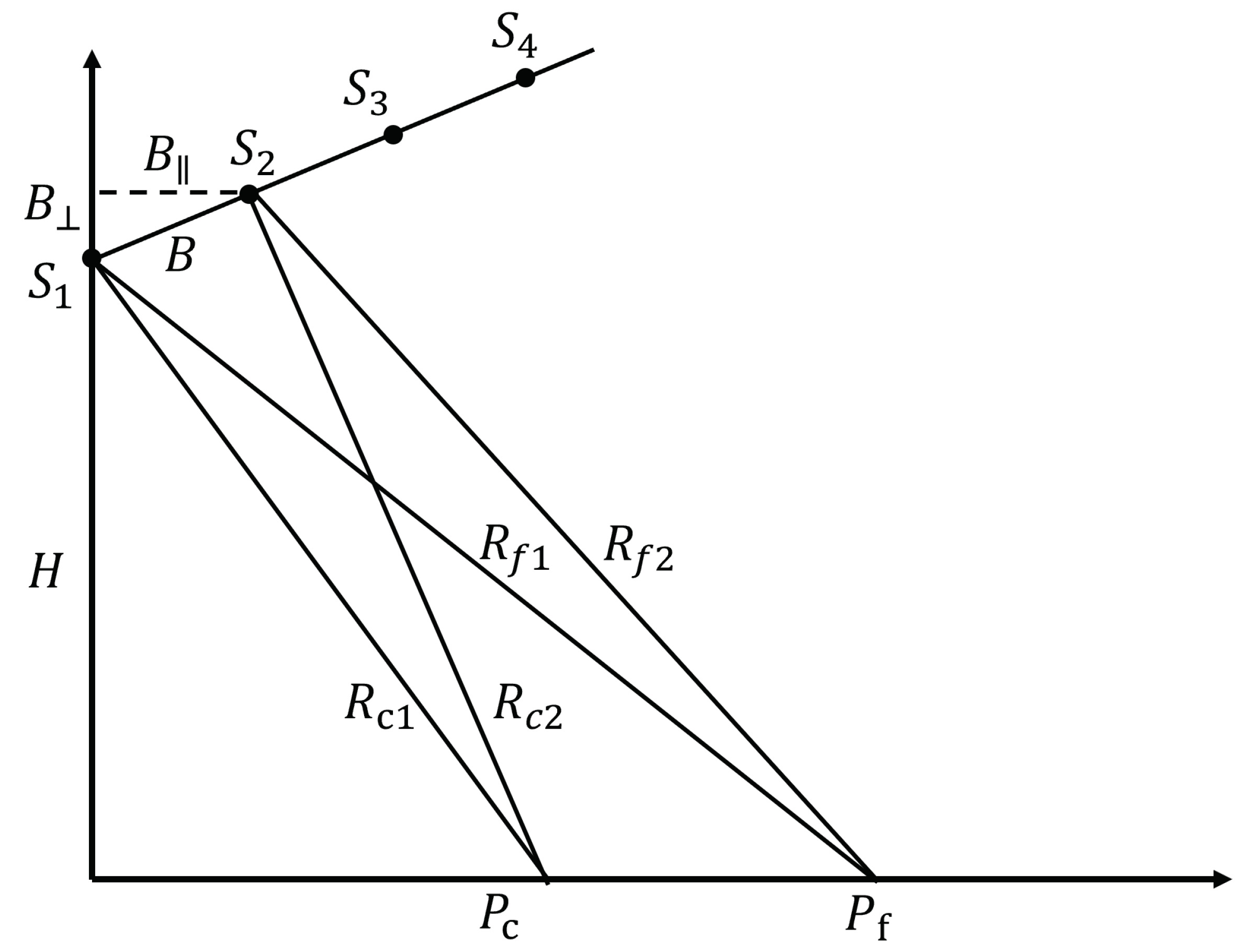
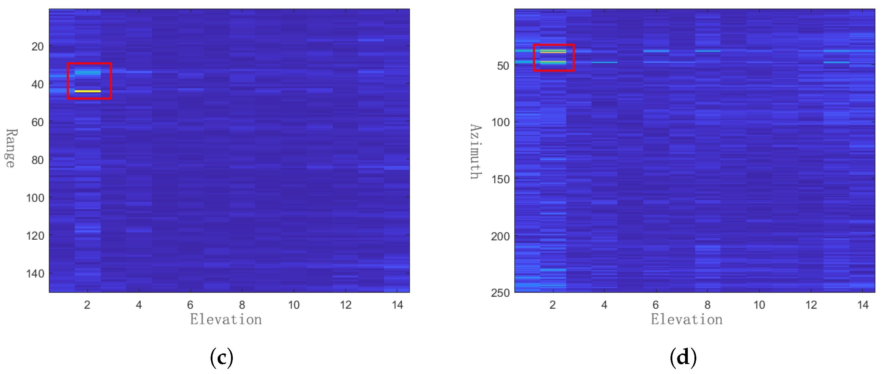
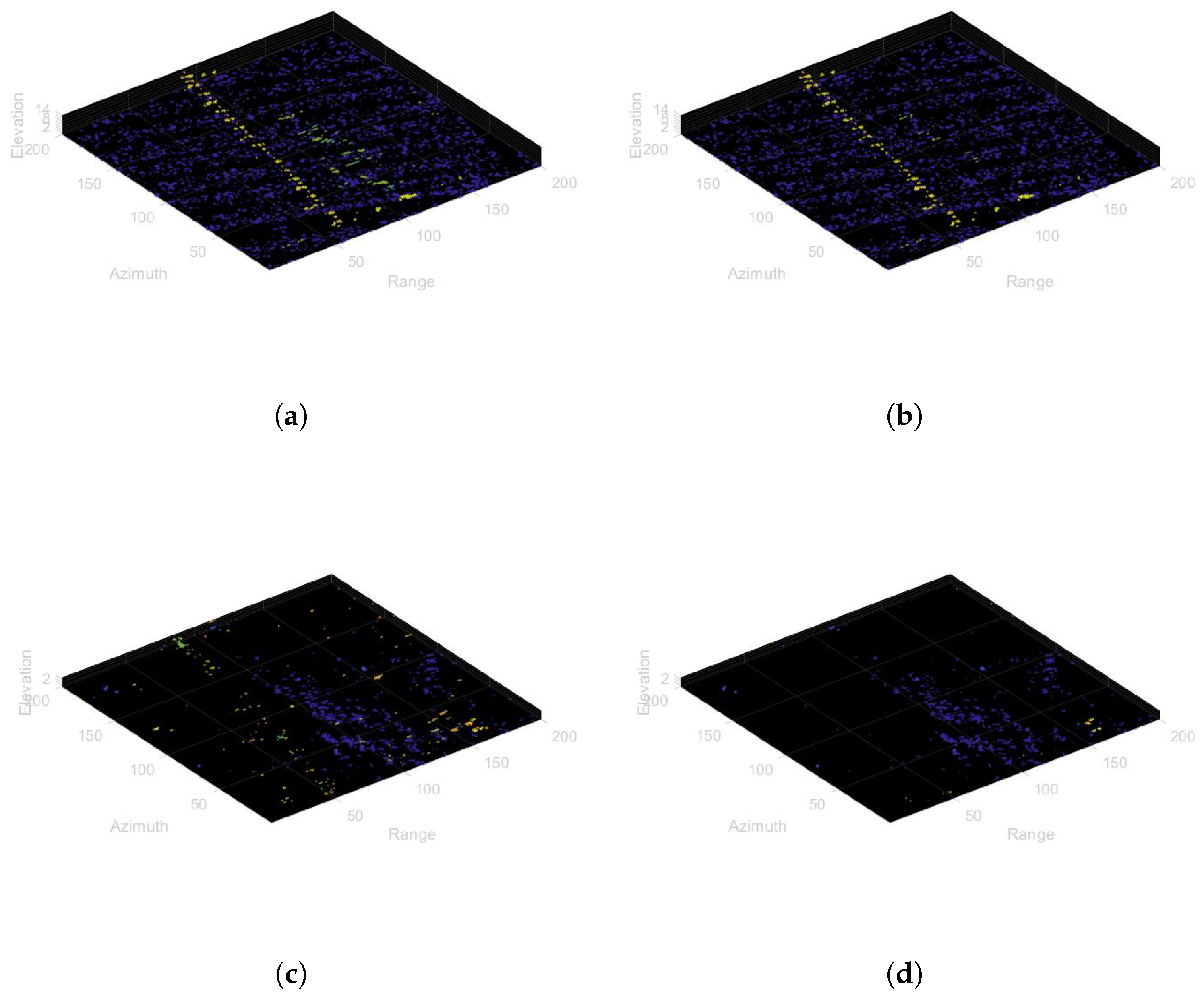
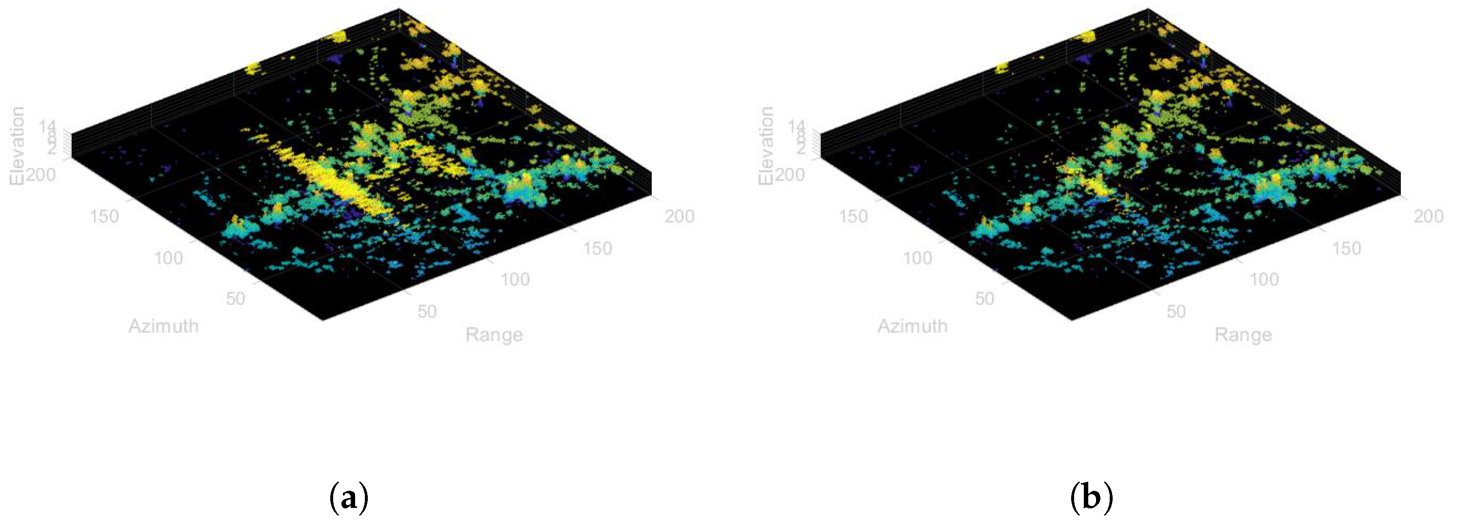
• Range de-ambiguity is carried out in 3D-space. By taking advantage of the characteristic that range ambiguity will cause further defocusing in the height direction, focused targets are selected, and the defocused point clouds are estimated and eliminated by using the focused targets to achieve range de-ambiguity.
• The phase errors existing in the process of estimating the defocused point clouds are analyzed. Part of these errors is introduced by the registration offset in the near-area and far-area images, and the other part is introduced during the transformation process between the near-area and far-area targets. Moreover, these errors have been corrected.

The rest of this paper is organized as follows: The method and principles are introduced in Section 2. The experimental data and results are provided in Section 3. Section 4 discusses the results of the method, as well as some potential applications, and finally, Section 5 concludes this paper.

2. Methods

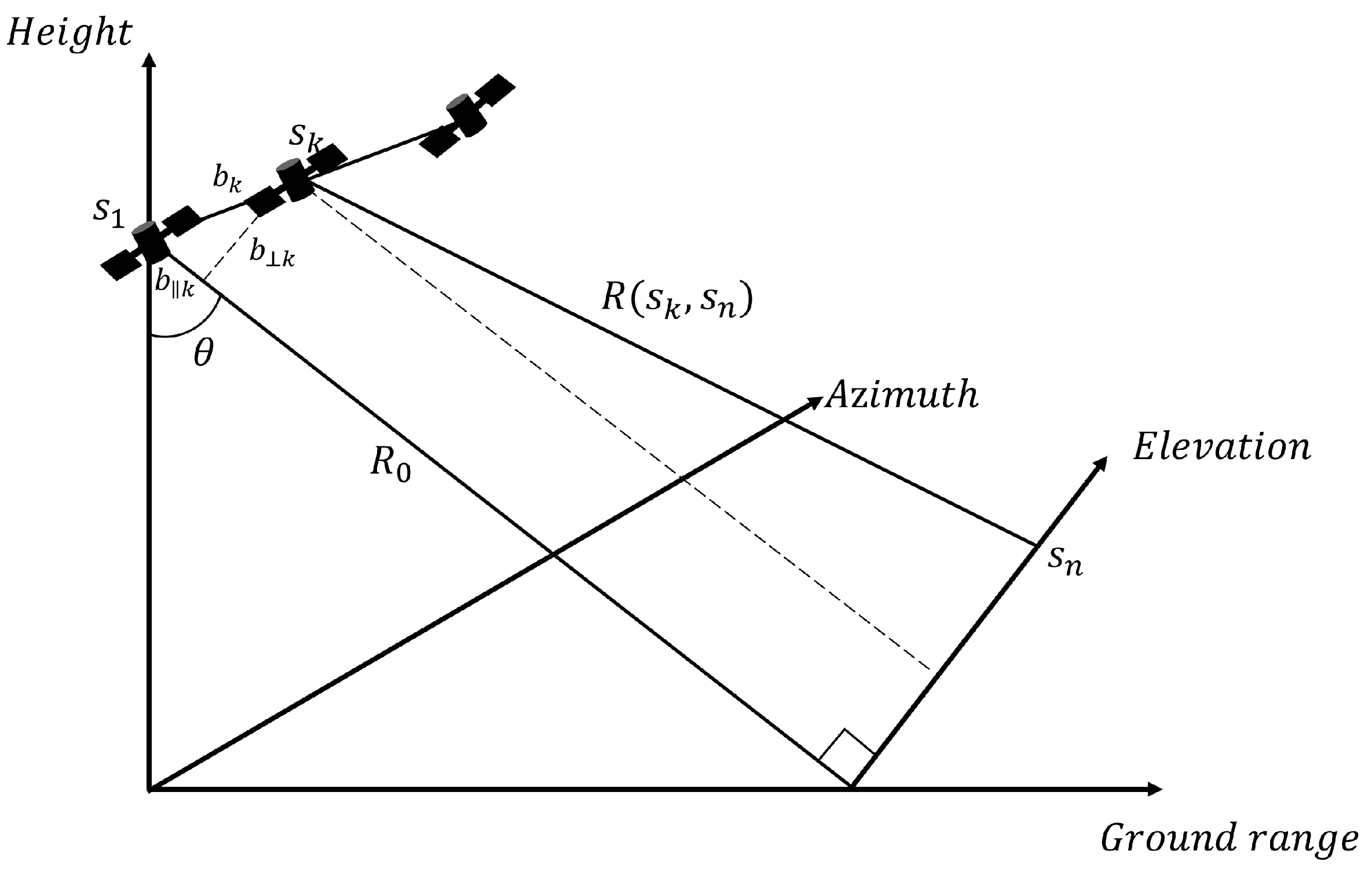
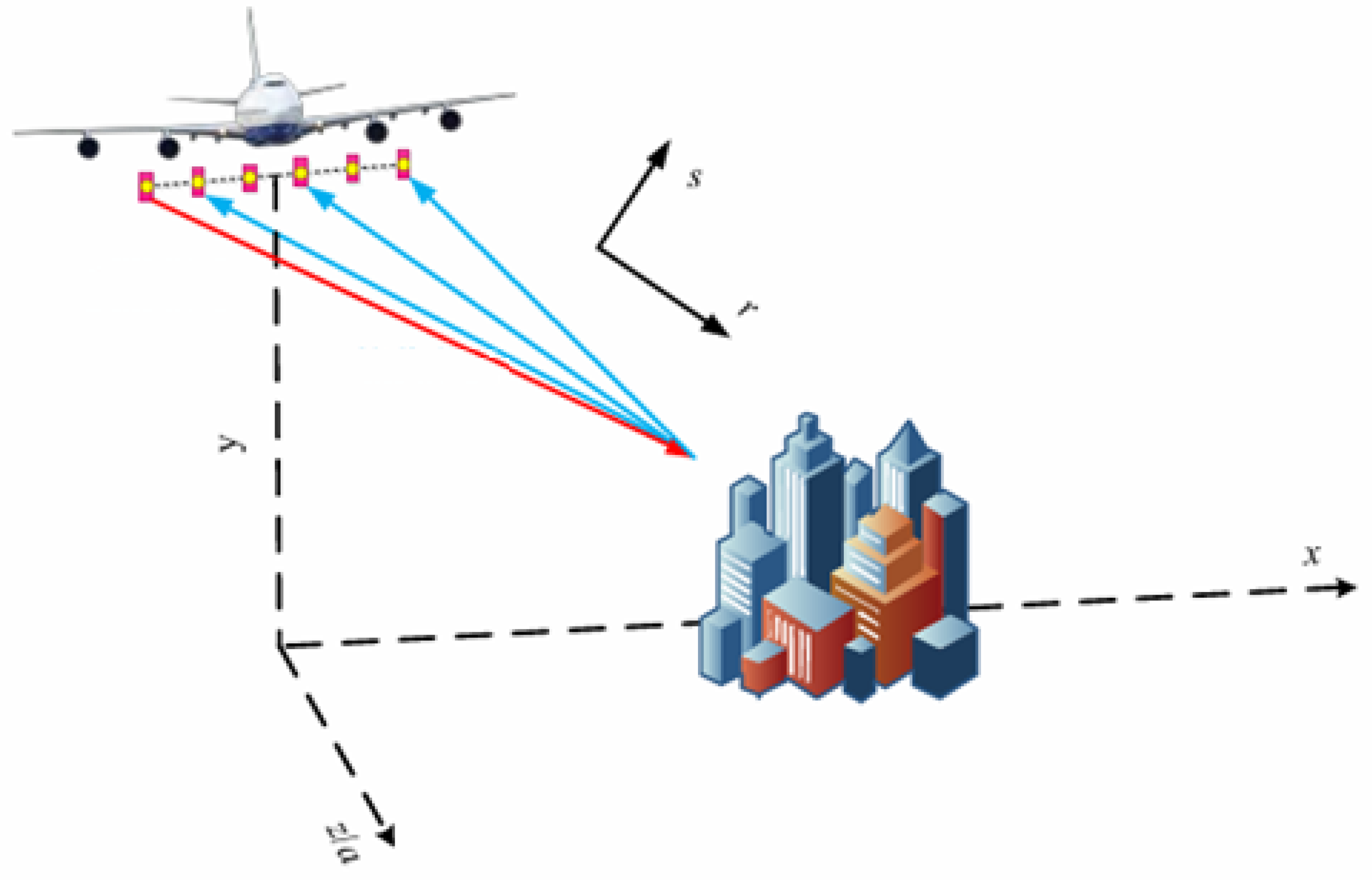
2.1. 3D-Imaging Principle of Distributed SAR System

Multi-channel SAR obtains height dimension resolution by adding antennas in the cross-track direction to form a virtual aperture. In a distributed SAR system, multiple satellite SARs are used to measure the same area from different angles and form a synthetic aperture in the elevation direction to achieve high-dimensional geometric resolution and realize true 3D-imaging. The distributed SAR multi-channel 3D-imaging system adopted in this paper has $N_k$ SAR received echoes, which are spatially distributed and arranged with baselines $b_{\perp k},k=0,\cdots ,N_{k-1}$ relative to the reference image.

To facilitate a more intuitive analysis of the layover phenomenon existing in multi-channel SAR, the capture geometry in the range-azimuth-height 3D plane is given as shown in Figure 1. The target at height $s_n$ and the ground target will fall within the same range-azimuth cell during the imaging process due to the same slant range, and the target cannot be resolved, that is, the layover phenomenon occurs.

After performing phase correction on the echo dataset, the received signals in each azimuth-range cell can be represented as the superposition of the backscattering intensities of all signals along the azimuth direction [36].

$$g\left(s_k\right)=\sum _n^{N_T}\gamma \left(s_n\right)e^{-j{\displaystyle \frac{4\pi }{\lambda }}R(s_k,s_n)}$$

(1)

Among them, $N_T$ represents the number of layover targets in the same azimuth-range cell, and $\gamma \left(s_n\right)$ represents the distribution of the backscattering coefficient in elevation. $s_n$ represents the height of the n-th layover target. $R(s_k,s_n)$, which represents the distance between the channel and the layover target, can be expanded by the Taylor series and approximated as:

$$R(s_k,s_n)=\sqrt{{(R_0-b_{\Vert k})}^2+{(b_{\perp k}-s_n)}^2}\approx R_0-b_{\Vert k}+{(b_{\perp k}-s_n)}^2/\left(2(R_0-b_{\Vert k})\right)$$

(2)

Since $R_0$ is a constant and can be neglected, and $b_{\Vert k}$, $s_k\ll R_0$, then Equation (1) can be expressed as:

$$\begin{array}{cc}\hfill \overline{g}\left(s_k\right)& =\sum _n^{N_T}\gamma \left(s_n\right)e^{-j{\displaystyle \frac{4\pi }{\lambda R_0}}{s}_n^2}{e}^{j{\displaystyle \frac{4\pi }{\lambda R_0}}{b}_{\perp k}{s}_n}=\sum _n^{N_T}\tilde{\gamma }\left(s_n\right)e^{j{\displaystyle \frac{4\pi }{\lambda R_0}}{b}_{\perp k}{s}_n}\hfill \end{array}$$

(3)

$$\begin{array}{cc}\hfill \tilde{\gamma }\left(s_n\right)& =\gamma \left(s_n\right)e^{-j{\displaystyle \frac{4\pi }{\lambda R_0}}{s}_n^2}\hfill \end{array}$$

(4)

Equation (3) indicates that the channel $s_k$ and the target elevation $s_n$ are Fourier transforms of each other. That is, on the premise that the system baseline interval satisfies the Nyquist sampling theorem, the scattering coefficient $\tilde{\gamma }\left(s_n\right)$ of the target scene can be retrieved by performing the inverse Fourier transform on the targets within the azimuth-range cells in the obtained SAR images.

2.2. 3D Blur Suppression Method

When the echoes with range ambiguity are focused in the near area and the far area, respectively, images with the near area focused and the far area blurred and images with the far area focused and the near area blurred will be obtained, respectively. In the images with the near area focused, the targets in the proximal area appear as focused bright points, while the targets in the distal area appear as a defocused patch of pixels. In the images with the far area focused, the targets in the distal area appear as focused bright points, while the targets in the proximal area appear as a defocused patch of pixels. The defocused targets will further defocus in 3D-space, while the focused targets will not.

Therefore, this paper proposes a 3D blur suppression method for HRWS blurred images. Firstly, image registration and phase compensation are performed on the multi-channel images with the far area focused and the near area blurred as well as those with the near area focused and the far area blurred. Then, Fourier transforms are conducted on the channel directions of the two sets of images, respectively, for elevation dimension focusing to obtain the 3D point clouds with the near area focused and the far area focused. Subsequently, the strong points are selected in the two sets of point clouds as the focused points, the defocused point clouds of these points are calculated in the other set of point clouds, and then the defocused point clouds are substracted from the other set of point clouds. Strong points continue to be selected from the remaining points and the same operations are performed until the defocused points in both the near-area focused and far-area focused point clouds are removed. Finally, those obtained are the unambiguous 3D point clouds in the near area and the far area, respectively, thus realizing 3D-imaging of blurred images. The specific scheme process is shown in Figure 2.

2.3. Calculation of Defocused Point Clouds

The key step of this method is the calculation of defocused point clouds. There are five steps in total for the calculation of defocused point clouds, and the specific process is shown in Figure 3.

• Inverse Fourier Transform (IFT) in the height direction

For the focused target point $(n_a,n_r,n_h)$, where $n_a$ represents the azimuth position, $n_r$ represents the range position, and $n_h$ represents the height position. Firstly, the IFT is performed in the elevation direction to restore the component of the focused point in the channel direction.

$$s=IFT\left\{S_h\right\}$$

(5)

Among them, $s_h$ is the signal of the focused point, and s is the component of the focused point in the channel direction.

2.

Azimuth Defocusing

The azimuth defocusing of points is calculated in each channel. The components of different channels are transformed to the azimuth frequency domain, then they are multiplied by the quadratic phase, and the IFT is performed to obtain the signals that are defocused in both the azimuth and channel directions. The specific calculation for the defocusing of the proximal targets is as follows:

$$\begin{array}{cc}\hfill S(f,k)& =\mathrm{FT}\left\{s(n_a,k)\right\}k=1,\cdots ,N_k{n}_a=1,\cdots ,N_a\hfill \end{array}$$

(6)

$$\begin{array}{cc}\hfill s_a(n_a,k)& =\mathrm{IFT}\left\{S(f,k)exp\left(-i\times 100\pi \times {\left({\displaystyle \frac{f}{N_a}}\right)}^2\right)\right\}\hfill \end{array}$$

(7)

The calculation of the defocusing of distal targets is as follows:

$$s_a(n_a,k)=\mathrm{IFT}\left\{S(f,k)exp\left(i\times 100\pi \times {\left({\displaystyle \frac{f}{N_a}}\right)}^2\right)\right\}$$

(8)

Among them, S is the signal in the azimuth frequency domain, $N_k$ is the number of channels, $N_a$ is the number of sampling points in the azimuth direction, and $s_a$ is the signal that is defocused in both the azimuth and channel directions.

3.

Range Offset and Sinc Defocusing

When registering the near-area focused and far-area blurred images as well as the far-area focused and near-area blurred images, in order to ensure the corresponding points of the two sets of images are located within the same range-azimuth cell, the near-area focused and far-area focused images are spliced into one set of images according to their positional relationships, and then registration is carried out with the proximal focused targets as the registration benchmark.

Performing registration according to the above steps can achieve a relatively good registration effect for proximal targets. However, for the registration of distal targets, there will be offsets in different channels in the range direction, as shown in Figure 4.

After registering according to the proximal targets, the offset $\Delta R$ of the distal targets relative to the proximal targets in the range direction can be calculated by the following steps: Taking the SAR image of the first channel as the registration benchmark, the range differences are first calculated between the different channels of the proximal targets and the distal targets and the first channel:

$$\begin{array}{cc}\hfill R_{ck}-R_{c1}& =\sqrt{{(\sqrt{(R_{c1}^2-H^2)}+B_{k\Vert })}^2+{(H+B_{k\perp })}^2}-R_{c1}\hfill \end{array}$$

(9)

$$\begin{array}{cc}\hfill R_{fk}-R_{f1}& =\sqrt{{(\sqrt{(R_{f1}^2-H^2)}+B_{k\Vert })}^2+{(H+B_{k\perp })}^2}-R_{f1}\hfill \end{array}$$

(10)

Among them, $R_{ck}$ represents the range difference between different channels of the proximal targets and the first channel, $R_{fk}$ represents the range difference between different channels of the distal targets and the first channel, H is the platform height, and $B_{\Vert }$ and $B_{\perp }$ are the horizontal and vertical components of the baseline of the k-th channel, respectively.

The offset $\Delta R$ of the distal targets relative to the proximal targets in the range direction can be expressed as follows:

$$\Delta R\left(k\right)=(R_{fk}-R_{f1})-(R_{ck}-R_{c1})$$

(11)

After calculating the registration offset in the range direction, it is necessary to calculate the defocusing in the range direction. The defocusing in the range direction can be regarded as the inverse process of sinc interpolation. In this paper, it is defocused by 8 pixels on each side in the range direction, and the weights at the corresponding positions after defocusing in the range direction are as follows:

$$\begin{array}{cc}\hfill w_{c-f}(m,k)& =\sin \mathrm{c}\left(m+{\displaystyle \frac{\Delta R\left(k\right)}{R_{\min }}}-⌊{\displaystyle \frac{\Delta R\left(k\right)}{R_{\min }}}⌋\right)m=-8,\cdots ,0,\cdots 8\hfill \end{array}$$

(12)

$$\begin{array}{cc}\hfill w_{f-c}(m,k)& =\sin \mathrm{c}\left(m-\left({\displaystyle \frac{\Delta R\left(k\right)}{R_{\min }}}-⌊{\displaystyle \frac{\Delta R\left(k\right)}{R_{\min }}}⌋\right)\right)\hfill \end{array}$$

(13)

Among them, $R_{\min }$ is the pixel width in the range direction, $w_{c-f}$ is the weight for calculating the distal defocused targets using the proximal focused targets, and $w_{f-c}$ is the weight for calculating the proximal defocused targets using the distal focused targets.

The values at the corresponding positions after defocusing are as follows:

$$\begin{array}{cc}\hfill s_{c-f}\left(n_a,n_r+m-⌊{\displaystyle \frac{\Delta R\left(k\right)}{R_{\min }}}⌋,k\right)& =s_a(n_a,n_r,k)\times w_{c-f}(m,k)\hfill \end{array}$$

(14)

$$\begin{array}{cc}\hfill s_{f-c}\left(n_a,n_r+m+⌊{\displaystyle \frac{\Delta R\left(k\right)}{R_{\min }}}⌋,k\right)& =s_a(n_a,n_r,k)\times w_{f-c}(m,k)\hfill \\ \hfill n_a=1,\cdots ,N_a{n}_r=1,\cdots ,N_r\end{array}$$

(15)

Among them, $N_r$ is the number of sampling points in the range direction, $s_{c-f}$ is the value for calculating the distal defocused targets using the proximal focused targets, and $s_{f-c}$ is the value for calculating the proximal defocused targets using the distal focused targets.

4.

Phase Error Compensation

After the above processes, the defocused signals of the near and far areas are basically calculated, but there are still some phase errors. Part of these errors is the phase error caused by the offset in the range direction, which can be expressed as:

$${\theta }_r\left(k\right)={\displaystyle \frac{4\pi \Delta R\left(k\right)}{\lambda }}$$

(16)

The other part is the phase error in the calculation process, which can be estimated by the phase error of the 2D image. Azimuth defocusing, range offset, and sinc interpolation are performed on the two-dimensional SAR image in one area to obtain the estimation of the image in the other area. The mean value is taken of the interference phase of the estimated image and the real image as the error in the calculation process. The specific calculation process for estimating the phase error of the far-area image from the near area is as follows:

$${\widehat{s}}_f(n_a,n_r,k)=\sum _{m=-8}^8{s}_a(n_a,n_r+m+⌊{\displaystyle \frac{\Delta R\left(k\right)}{R_{\min }}}⌋,k)\times \sin \mathrm{c}\left(m-\left({\displaystyle \frac{\Delta R\left(k\right)}{R_{\min }}}-⌊{\displaystyle \frac{\Delta R\left(k\right)}{R_{\min }}}⌋\right)\right)\times exp\left({\theta }_r\left(k\right)\right)$$

(17)

$${\theta }_{c-f}\left(k\right)=\mathrm{angle}\left({\displaystyle \frac{1}{N_a\times N_r}}\sum _{n_a=1}^{N_a}\sum _{n_r=1}^{N_r}{\widehat{s}}_f(n_a,n_r,k)\times s^{*}\right)$$

(18)

The specific calculation process for estimating the phase error of the near-area image from the far area is as follows:

$${\widehat{s}}_f(n_a,n_r,k)=\sum _{m=-8}^8{s}_a(n_a,n_r+m-⌊{\displaystyle \frac{\Delta R\left(k\right)}{R_{\min }}}⌋,k)\times \sin \mathrm{c}\left(m+\left({\displaystyle \frac{\Delta R\left(k\right)}{R_{\min }}}-⌊{\displaystyle \frac{\Delta R\left(k\right)}{R_{\min }}}⌋\right)\right)\times exp(-{\theta }_r\left(k\right))$$

(19)

$${\theta }_{f-c}\left(k\right)=\mathrm{angle}\left({\displaystyle \frac{1}{N_a\times N_r}}\sum _{n_a=1}^{N_a}\sum _{n_r=1}^{N_r}{\widehat{s}}_f(n_a,n_r,k)\times s^{*}\right)$$

(20)

Among them, $s_a$ has been mentioned above, ${\theta }_{c-f}$ and ${\theta }_{f-c}$ are the phase errors of the defocused near-area and far-area targets, respectively.

The defocused signals after removing the phase errors are as follows:

$$\begin{array}{cc}\hfill {\widehat{s}}_{c-f}\left(k\right)& =s_{c-f}\left(k\right)\times exp\left({\theta }_r\left(k\right)\right)\times exp(-{\theta }_{c-f}\left(k\right))\hfill \end{array}$$

(21)

$$\begin{array}{cc}\hfill {\widehat{s}}_{f-c}\left(k\right)& =s_{f-c}\left(k\right)\times exp(-{\theta }_r\left(k\right))\times exp(-{\theta }_{f-c}\left(k\right))\hfill \end{array}$$

(22)

5.

Fourier Transform (FT) in the channel direction

Finally, the Fourier transform is performed in the channel direction and the signal is converted back to the height direction, so that the defocused point cloud of the near-area target and the far-area target in the 3D-space can be obtained.

$$\begin{array}{cc}\hfill S_{c-f}& =FT\left\{{\widehat{s}}_{c-f}\left(k\right)\right\}\hfill \end{array}$$

(23)

$$\begin{array}{cc}\hfill S_{f-c}& =FT\left\{{\widehat{s}}_{f-c}\left(k\right)\right\}\hfill \end{array}$$

(24)

3. Experiments and Results

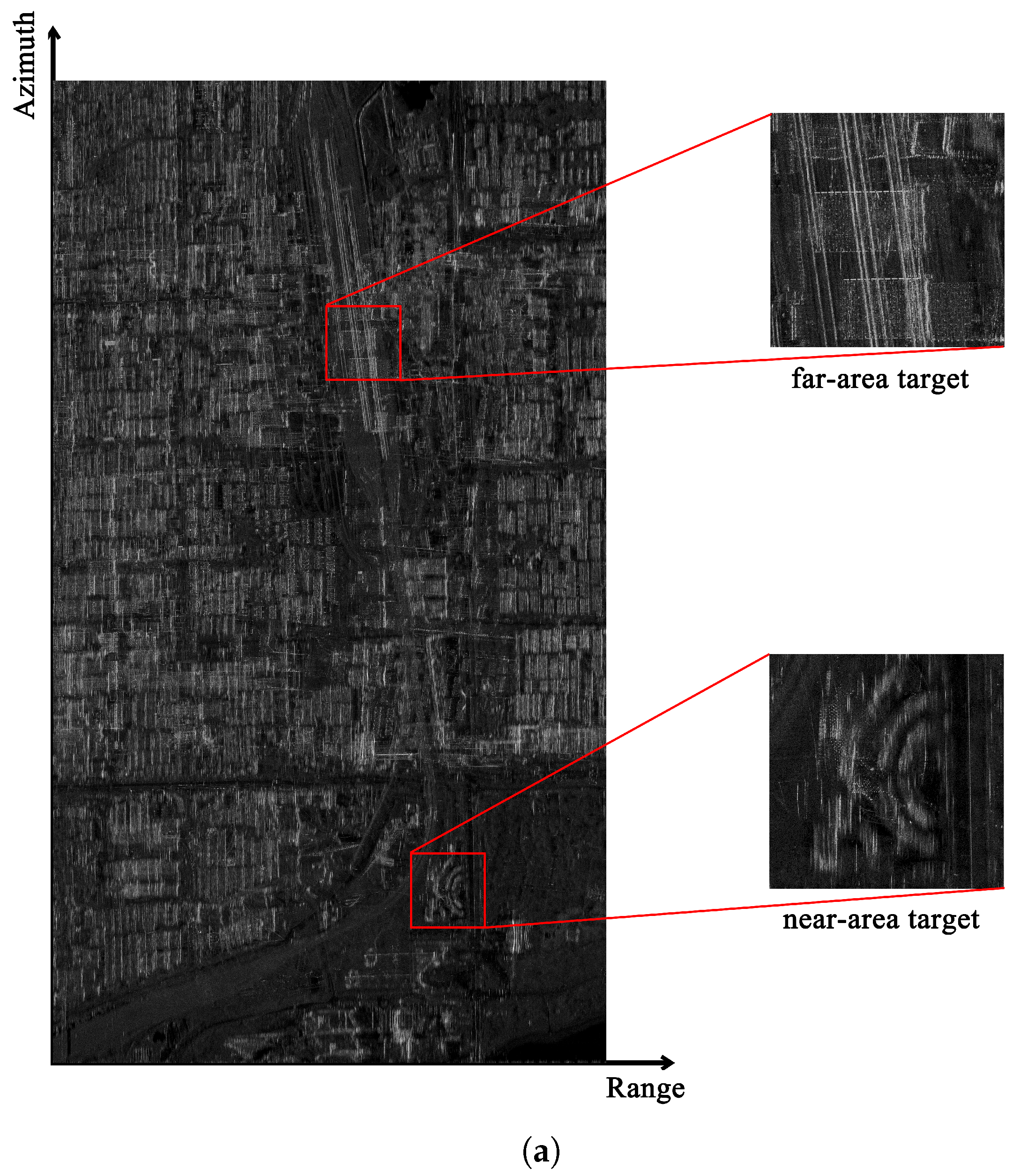
3.1. Study Area and Data

The experimental system in this experiment is the mechanism array tomography SAR system developed by the Aerospace Information Research Institute of the Chinese Academy of Sciences (AIRCAS). Its schematic diagram is shown in Figure 5, and it is a multi-transmit and multi-receive mechanism. The data selected are the original urban area data obtained by our team in 2021 in Rizhao City, Shandong Province, China. The optical image of the target area is shown in Figure 6, and the detailed parameters of the experimental system are listed in

Table 1. Main parameters of the experimental system.

Parameter	Value
Center frequency	10 GHz
Flight height	5 km
Bandwidth	500 MHz
Baseline length	2.0 m
Baseline interval	0.2 m
The horizontal inclination of the baseline	0°
Central incidence angle	35°

.

3.2. Experimental Results

The experimental data in this test are the airborne array tomography SAR data of the urban area in Rizhao City, Shandong Province. The acquired airborne data do not contain range ambiguities, so it is necessary to simulate range ambiguities first. In this paper, after adding range ambiguities to the original echo in a semi-physical manner, 2D SAR imaging was carried out in the near area and the far area, respectively, and two sets of imaging results of the target area were obtained, as shown in Figure 7. As analyzed above, an excessively high PRF of the radar will cause range ambiguities. By comparing Figure 7 with Figure 6, it can be intuitively seen that the targets in the distance and those in the vicinity are superimposed together after range ambiguities occur. Among them, different buildings, buildings and roads, as well as buildings and the ground, are all superimposed on each other, and it is difficult to distinguish the targets from the ambiguous signals. Moreover, the near-area targets enclosed in the box in Figure 7a are in focus, while the far-area targets are out of focus. In contrast, the corresponding near-area targets enclosed in the box in Figure 7b appear out of focus, and the far-area targets appear in focus.

The image obtained by splicing the two sets of images according to their positional relationship is shown in Figure 8. Using the proximal targets as the registration benchmark, the spliced image is registered and the amplitude and phase error compensation is carried out. Then, the regions within the boxes in the near-area and far-area images are selected for height-direction focusing, and the near-area focused and far-area blurred point cloud as well as the far-area focused and near-area blurred point cloud are generated, respectively.

The phase error in the process of near-area and far-area image conversion is shown in Figure 9. Taking channel 1 as the registration reference, it can be observed that as the distance from channel 1 increases, the existing phase error basically becomes larger as well, which is in line with the reasoning above.

The results of phase error correction are shown in Figure 10. Figure 10a,b display the interferometric phases of the estimated image and the original image before the transformation phase error correction. The average interferometric phase of the near-end image is approximately $0.8$, and the average interferometric phase of the far-end image is approximately $-0.7$. Figure 10c,d present the interferometric phases of the estimated image and the original image after the transformation phase error correction. The average interferometric phases of the two images are almost zero. It can be seen that most of the phase error has been corrected except for the edge regions.

The processed point cloud is shown in Figure 11. It can be seen that whether it is in the near area or the far area, the blurred point cloud has been removed while the focused point cloud has been retained. In Figure 11, a set of near-area point targets, a set of far-area point targets, and a set of near-area zone targets were selected for analysis. After magnifying the three sets of targets in the red box of Figure 11, Figure 12 is obtained. The two near-area point targets in Figure 12a are presented as blurred point clouds in the far-area image, as shown in Figure 12b. The blurred point clouds are blurred to varying degrees in the azimuth direction, range direction, and height direction. The result of blurring suppression using the method proposed in this paper is shown in Figure 12c, and it can be observed that the blurred point clouds are eliminated. The three far-area point targets in Figure 12d are presented as blurred point clouds in the near-area image, as shown in Figure 12e. The result of blurring suppression is shown in Figure 12f, and it can be observed that the blurred point clouds are eliminated. The near-area zone targets in Figure 12g are presented as blurred point clouds in the far-area image, as shown in Figure 12h. The original zone targets are blurred into a mass, and it is completely impossible to discern the target structure from it. The result of blurring suppression is shown in Figure 12i, and it can be observed that the blurred point clouds are basically eliminated.

The image obtained by superimposing the processed point cloud along the range direction and the azimuth direction is shown in Figure 13. The targets outlined in the figure were submerged in the blurred point clouds before processing. However, after applying the blurring suppression method proposed in this paper, these targets became visible. It can be seen that the blurred signals have been removed and the focused signals have been retained.

As the experimental results obtained through the method proposed in this paper are in the form of 3D point clouds, this paper employs the proportion of eliminated blurred point clouds as an objective evaluation metric to quantify the effectiveness of blurring suppression. The detailed formula is presented as follows:

$$R={\displaystyle \frac{(n_{origin}-n_{clear})-(n_{result}-n_{clear})}{(n_{origin}-n_{clear})}}$$

(25)

Among them, $n_{origin}$ represents the number of points in the original point cloud, which includes both blurred point clouds and clear point clouds, $n_{clear}$ represents the number of points in the clear point cloud, and $n_{result}$ represents the number of points in the processed point cloud, which contains residual blurred point clouds and clear point clouds.

The proportion of eliminated blurred point clouds in the experimental area is shown in

Table 2. The proportion of eliminated blurred point clouds in the experimental area.

Near Area	Far Area
87.2%	92.6%

. Among them, the proportion of eliminated blurred point clouds in the near area of the experimental area is 87.2%, and that in the far area is 92.6%. Most of the blurred point clouds have been eliminated, which demonstrates the effectiveness of this method.

In addition, we specifically selected two sets of data from vegetated areas and water areas for experiments. The experimental results for the vegetated area are shown in Figure 14. The vegetation is located in the far area, and the corresponding target in the near area is a section of road. As can be seen from Figure 14b,d, the ambiguous point clouds are basically eliminated, and the clear point clouds of the vegetation and the road are restored. There are few targets in the water area. Therefore, the ambiguous signals in the corresponding area generate relatively few ambiguous point clouds. Meanwhile, most of the ambiguous point clouds formed by the blurred signals in the water area are not located at the same positions as the clear point clouds. So, the ambiguity suppression effect is better. The experimental results for the water area are shown in Figure 15. The near-area target is the roof part of a high-rise building, and the far-area target is the water area with a boat on the water surface. As can be seen from Figure 15b,d, the ambiguous point clouds are basically eliminated. The boat originally covered by the ambiguous point clouds is revealed, and the building roof also becomes clear.

4. Discussion

When the echoes with range ambiguity are focused in the near area and the far area, respectively, images with the near area focused and the far area blurred, and images with the far area focused and the near area blurred will be obtained, respectively. In the near-area focused image, the proximal targets appear as focused strong points, while the far-area targets blurred in the near-area image appear as a defocused patch of pixels. In the far-area focused image, the far-area targets appear as focused strong points, while the near-area targets blurred in the far-area image appear as a defocused patch of pixels.

The range ambiguity existing in the spaceborne distributed HRWS SAR system will lead to the simultaneous presence of focused point clouds and blurred point clouds in the generated 3D point clouds, which seriously affects the quality of the 3D point clouds. Blurred targets will be further defocused in 3D-space, while focused targets will not. Therefore, in this study, a 3D blur suppression method for distributed HRWS SAR blurred images based on estimating and eliminating defocused point clouds from focused point clouds is proposed. Different from previous range de-ambiguity methods, this method innovatively discusses range de-ambiguity in 3D-space. First, 3D-imaging is performed on the observed scene, the focused points in the 3D-space are directly searched for and retained, and the focused points in one area are used to estimate and eliminate the blurred point clouds in the other area, so as to obtain unambiguous 3D point clouds and simultaneously achieve high-resolution wide-swath imaging and 3D-imaging.

The estimation of blurred point clouds requires undergoing inverse Fourier transform in the height direction, defocusing in the azimuth direction, offsetting in the range direction, and sinc defocusing first, then performing phase error correction, and finally, performing Fourier transform in the channel direction to estimate the blurred point clouds. Phase errors include errors introduced by registration offsets and phase errors existing in the conversion process. The phase errors introduced by registration offsets can be calculated through the SAR geometric relationship, and the phase errors existing in the conversion process can be estimated through the phase errors of the conversion of 2D images.

In the experimental part of Section 3, experiments were carried out using the measured data from airborne flights and by simulating SAR images with range ambiguity. After performing 3D-imaging according to the method proposed in this paper, both focused targets and defocused blurred point clouds can be observed simultaneously in the experimental area. After range de-ambiguity, it can be clearly observed that the blurred point clouds are basically eliminated, and the focused point clouds are retained as targets. By superimposing the processed point clouds along the range direction and the azimuth direction, it can be clearly seen that the targets that were originally blurred in the point clouds become clear, indicating that the method proposed in this paper can effectively eliminate the impact of range ambiguity on 3D-imaging and achieve HRWS 3D-imaging.

5. Conclusions

The distributed HRWS system transmits signals with a high PRF which will lead to range ambiguity in large detection scenarios. To address this issue, this paper proposes a 3D blur suppression method for distributed HRWS SAR images with ambiguity, which estimates and eliminates defocused point clouds with focused point clouds. Firstly, 3D-imaging is performed on the observed scene to generate the 3D point clouds of the scene. Then, the focused points in the 3D-space are search for and retained, and the focused points in one area are used to estimate and eliminate the blurred point clouds in the other area, so as to obtain unambiguous 3D point clouds and achieve HRWS 3D-imaging. Simulation experiments based on airborne measured data proved that the method in this paper can effectively eliminate the blurred point clouds in the 3D point clouds and has the capability of HRWS 3D-imaging.

References

1. Goodman, N.; Lin, S.C.; Rajakrishna, D.; Stiles, J. Processing of multiple-receiver spaceborne arrays for wide-area SAR. IEEE Trans. Geosci. Remote Sens. 2002, 40, 841–852. [Google Scholar] [CrossRef]
2. Das, A.; Cobb, R.G.; Stallard, M. Techsat 21—A revolutionary concept in distributed space based sensing. In Proceedings of the AIAA Defense and Civil Space Programs Conference and Exhibit, Huntsville, AL, USA, 28–30 October 1998. [Google Scholar] [CrossRef]
3. Martin, M.; Stallard, M. Distributed satellite missions and technologies—The TechSat 21 program. In Proceedings of the Space Technology Conference and Exposition, Albuquerque, NM, USA, 28–30 September 1999. [Google Scholar] [CrossRef]
4. Jilla, C.; Miller, D. A Multiobjective, Multidisciplinary Design Optimization Methodology for the Conceptual Design of Distributed Satellite Systems. In Proceedings of the 9th AIAA/ISSMO Symposium on Multidisciplinary Analysis and Optimization, Atlanta, GA, USA, 4–6 September 2002. [Google Scholar] [CrossRef]
5. Burns, R.; McLaughlin, C.; Leitner, J.; Martin, M. TechSat 21: Formation design, control, and simulation. In Proceedings of the 2000 IEEE Aerospace Conference, Big Sky, MT, USA, 18–25 March 2000. [Google Scholar] [CrossRef]
6. Girard, R.; Séguin, G. The RADARSAT-2 & 3 interferometric mission. In Proceedings of the 2002 9th International Symposium on Antenna Technology and Applied Electromagnetics, St. Hubert, QC, Canada, 31 July–2 August 2002; pp. 1–4. [Google Scholar]
7. Lee, P.; James, K. The RADARSAT-2/3 topographic mission. In Proceedings of the IEEE 2001 International Geoscience and Remote Sensing Symposium, Scanning the Present and Resolving the Future, Sydney, NSW, Australia, 9–13 July 2001; Proceedings (Cat. No.01CH37217). IEEE: New York, NY, USA, 2001; Volume 1, pp. 499–501. [Google Scholar] [CrossRef]
8. Cote, S.; Lapointe, M.; De Lisle, D.; Arsenault, E.; Wierus, M. The RADARSAT Constellation: Mission Overview and Status. In Proceedings of the EUSAR 2021, 13th European Conference on Synthetic Aperture Radar, Online, 29 March–1 April 2021; pp. 1–5. [Google Scholar]
9. Moro, M.; Chini, M.; Saroli, M.; Atzori, S.; Stramondo, S.; Salvi, S. Analysis of large, seismically induced, gravitational deformations imaged by high-resolution COSMO-SkyMed synthetic aperture radar. Ann. Biol. Clin. 2011, 39, 527–530. [Google Scholar] [CrossRef]
10. Massonnet, D. Capabilities and limitations of the interferometric cartwheel. IEEE Trans. Geosci. Remote Sens. 2001, 39, 506–520. [Google Scholar] [CrossRef]
11. Massonnet, D. The interferometric cartwheel: A constellation of passive satellites to produce radar images to be coherently combined. Int. J. Remote Sens. 2001, 22, 2413–2430. [Google Scholar] [CrossRef]
12. Romeiser, R. On the suitability of a TerraSAR-L Interferometric Cartwheel for ocean current measurements. In Proceedings of the IGARSS 2004—2004 IEEE International Geoscience and Remote Sensing Symposium, Anchorage, AK, USA, 20–24 September 2004; Volume 5, pp. 3345–3348. [Google Scholar] [CrossRef]
13. Mittermayer, J.; Krieger, G.; Moreira, A.; Wendler, M. Interferometric performance estimation for the interferometric Cartwheel in combination with a transmitting SAR-satellite. In Proceedings of the IEEE 2001 International Geoscience and Remote Sensing Symposium, Scanning the Present and Resolving the Future, Sydney, NSW, Australia, 9–13 July 2001; Proceedings (Cat. No.01CH37217). IEEE: New York, NY, USA, 2001; Volume 7, pp. 2955–2957. [Google Scholar] [CrossRef]
14. Ebner, H.; Riegger, S.; Hajnsek, I.; Hounam, D.; Krieger, G.; Moreira, A.; Werner, M. Single-Pass SAR Interferometry with a Tandem TerraSAR-X Configuration. In Proceedings of the EUSAR 2004, Ulm, Germany, 25–27 May 2004; VDE/ITG, Ed.; VDE: San Jose, CA, USA, 2004; Volumes 1 and 2, p. 53. [Google Scholar]
15. Krieger, G.; Moreira, A.; Fiedler, H.; Hajnsek, I.; Werner, M.; Younis, M.; Zink, M. TanDEM-X: A Satellite Formation for High-Resolution SAR Interferometry. IEEE Trans. Geosci. Remote Sens. 2007, 45, 3317–3341. [Google Scholar] [CrossRef]
16. Fiedler, H.; Krieger, G.; Werner, M.; Reiniger, K.; Eineder, M.; D’Amico, S.; Diedrich, E.; Wickler, M. The TanDEM-X Mission Design and Data Acquisition Plan. In Proceedings of the European Conference on Synthetic Aperture Radar (EUSAR), Dresden, Germany, 16–18 May 2006; VDE, Ed.; VDE: San Jose, CA, USA, 2006; p. 4. [Google Scholar]
17. Sanfourche, J.P. ‘SAR-lupe’, an important German initiative. Air Space Eur. 2000, 2, 26–27. [Google Scholar] [CrossRef]
18. Mou, J.; Wang, Y.; Fu, X.; Guo, S.; Lu, J.; Yang, R.; Ma, X.; Hong, J. Initial Results of Geometric Calibration of Interferometric Cartwheel SAR HT-1. In Proceedings of the IGARSS 2024—2024 IEEE International Geoscience and Remote Sensing Symposium, Athens, Greece, 7–12 July 2024; pp. 8886–8890. [Google Scholar] [CrossRef]
19. Callaghan, G.D.; Longstaff, I.D. Wide-swath space-borne SAR using a quad-element array. IEE Proc.—Radar Sonar Navig. 1999, 146, 159–165. [Google Scholar] [CrossRef]
20. Bordoni, F.; Younis, M.; Varona, E.M.; Gebert, N.; Krieger, G. Performance Investigation on Scan-On-Receive and Adaptive Digital Beam-Forming for High-Resolution Wide-Swath Synthetic Aperture Radar. In Proceedings of the International ITG Workshop of Smart Antennas, Berlin, Germany, 16–18 February 2009; EURASIP, Ed.; Informationstechnische Gesellschaft im VDE, ITG: San Jose, CA, USA, 2009; pp. 114–121. [Google Scholar]
21. Gebert, N.; Krieger, G.; Moreira, A. Digital Beamforming on Receive: Techniques and Optimization Strategies for High-Resolution Wide-Swath SAR Imaging. IEEE Trans. Aerosp. Electron. Syst. 2009, 45, 564–592. [Google Scholar] [CrossRef]
22. Suess, M.; Grafmueller, B.; Zahn, R. A novel high resolution, wide swath SAR system. In Proceedings of the IEEE 2001 International Geoscience and Remote Sensing Symposium, Scanning the Present and Resolving the Future, Sydney, NSW, Australia, 9–13 July 2001; Proceedings (Cat. No.01CH37217). Volume 3, pp. 1013–1015. [Google Scholar] [CrossRef]
23. Makhoul Varona, E. Adaptive Digital Beam-Forming for High-Resolution Wide-Swath Synthetic Aperture Radar. Ph.D. Thesis, UPC, Escola Tècnica Superior d’Enginyeria de Telecomunicació de Barcelona, Departament de Teoria del Senyal i Comunicacions, Barcelona, Spain, 2009. [Google Scholar]
24. Liu, B.; He, Y. Improved DBF Algorithm for Multichannel High-Resolution Wide-Swath SAR. IEEE Trans. Geosci. Remote Sens. 2016, 54, 1209–1225. [Google Scholar] [CrossRef]
25. Xie, H.; Gao, Y.; Dang, X.; Tan, X.; Li, S.; Chang, X. A robust DBF method for Spaceborne SAR. In Proceedings of the 2019 IEEE International Conference on Signal, Information and Data Processing (ICSIDP), Chongqing, China, 11–13 December 2019; pp. 1–4. [Google Scholar] [CrossRef]
26. Ye, S.; Yang, T.; Li, W. A Novel Algorithm for Spacebome SAR DBF Based on Sparse Spatial Spectrum Estimation. In Proceedings of the 2018 China International SAR Symposium (CISS), Shanghai, China, 10–12 October 2018; pp. 1–4. [Google Scholar] [CrossRef]
27. Yang, Y.; Zhang, F.; Tian, Y.; Chen, L.; Wang, R.; Wu, Y. High-Resolution and Wide-Swath 3D Imaging for Urban Areas Based on Distributed Spaceborne SAR. Remote Sens. 2023, 15, 3938. [Google Scholar] [CrossRef]
28. Wang, W.Q. Range-Angle Dependent Transmit Beampattern Synthesis for Linear Frequency Diverse Arrays. IEEE Trans. Antennas Propag. 2013, 61, 4073–4081. [Google Scholar] [CrossRef]
29. Xu, J.; Liao, G.; Zhu, S. Receive beamforming of frequency diverse array radar systems. In Proceedings of the 2014 XXXIth URSI General Assembly and Scientific Symposium (URSI GASS), Beijing, China, 16–23 August 2014; pp. 1–4. [Google Scholar] [CrossRef]
30. Sammartino, P.F.; Baker, C.J.; Griffiths, H.D. Frequency Diverse MIMO Techniques for Radar. IEEE Trans. Aerosp. Electron. Syst. 2013, 49, 201–222. [Google Scholar] [CrossRef]
31. Wang, W.Q.; So, H.C.; Shao, H. Nonuniform Frequency Diverse Array for Range-Angle Imaging of Targets. IEEE Sens. J. 2014, 14, 2469–2476. [Google Scholar] [CrossRef]
32. Wei, J.; Li, Y.; Sun, Z. A Range Ambiguity Resolution Method for High-Resolution and Wide-Swath SAR Imaging Based on Continuous Pulse Coding. In Proceedings of the 2021 CIE International Conference on Radar (Radar), Hainan, China, 15–19 December 2021; pp. 211–214. [Google Scholar] [CrossRef]
33. Wen, X.; Qiu, X.; Han, B.; Ding, C.; Lei, B.; Chen, Q. A Range Ambiguity Suppression Processing Method for Spaceborne SAR with Up and Down Chirp Modulation. Sensors 2018, 18, 1454. [Google Scholar] [CrossRef] [PubMed]
34. Chang, S.; Deng, Y.; Zhang, Y.; Zhao, Q.; Wang, R.; Zhang, K. An Advanced Scheme for Range Ambiguity Suppression of Spaceborne SAR Based on Blind Source Separation. IEEE Trans. Geosci. Remote Sens. 2022, 60, 5230112. [Google Scholar] [CrossRef]
35. Chang, S.; Deng, Y.; Zhang, Y.; Zhao, Q.; Wang, R.; Jia, X. An Advanced Scheme for Range Ambiguity Suppression of Spaceborne SAR Based on Cocktail Party Effect. In Proceedings of the IGARSS 2022—2022 IEEE International Geoscience and Remote Sensing Symposium, Kuala Lumpur, Malaysia, 17–22 July 2022; pp. 2075–2078. [Google Scholar] [CrossRef]
36. Budillon, A.; Evangelista, A.; Schirinzi, G. Three-Dimensional SAR Focusing From Multipass Signals Using Compressive Sampling. IEEE Trans. Geosci. Remote Sens. 2011, 49, 488–499. [Google Scholar] [CrossRef]
Figure 1. Capture geometry of multi-channel SAR.
Remotesensing 17 00928 g001
Figure 2. Research scheme of the 3D blur suppression method for HRWS blurred images.
Remotesensing 17 00928 g002
Figure 3. Flow chart of defocused point cloud calculation.
Remotesensing 17 00928 g003
Figure 4. Range offset in different channels.
Remotesensing 17 00928 g004
Figure 5. Schematic diagram of the experimental system.
Remotesensing 17 00928 g005
Figure 6. Optical image of the experimental area.
Remotesensing 17 00928 g006
Figure 7. 2D SAR images after adding range ambiguities. (a) Image with near-area focusing and far-area blurring; (b) Image with far-area focusing and near-area blurring.
Remotesensing 17 00928 g007aRemotesensing 17 00928 g007b
Figure 8. Spliced SAR image.
Remotesensing 17 00928 g008
Figure 9. Phase error in the process of near-area and far-area image conversion. (a) Phase error of the far area estimated by the near area; (b) Phase error of the near area estimated by the far area.
Remotesensing 17 00928 g009
Figure 10. Interference phase of the estimated image and the original image. (a) Near area before phase error correction; (b) Far area before phase error correction; (c) Near area after phase error correction; (d) Far area after phase error correction.
Remotesensing 17 00928 g010
Figure 11. Experimental results. (a) Original point cloud in the near area; (b) Point cloud in the near area after deblurring; (c) Original point cloud in the far area; (d) Point cloud in the far area after deblurring.
Remotesensing 17 00928 g011
Figure 12. Analysis of experimental results for three groups of targets. (a) Point targets in the near area; (b) Blurred point clouds of near-area point targets; (c) Experimental result of near-area point targets; (d) Point targets in the far area; (e) Blurred point clouds of far-area point targets; (f) Experimental result of far-area point targets; (g) Zone targets in the far area; (h) Blurred point clouds of near-area zone targets; (i) Experimental result of near-area zone targets.
Remotesensing 17 00928 g012
Figure 13. Image after the point cloud is superimposed along the range direction and the azimuth direction. (a) Image superimposed along the azimuth before processing; (b) Image superimposed along the range before processing; (c) Image superimposed along the azimuth after processing; (d) Image superimposed along the range after processing.
Remotesensing 17 00928 g013aRemotesensing 17 00928 g013b
Figure 14. Experimental results in vegetated area. (a) Original point cloud in the near area; (b) Point cloud in the near area after deblurring; (c) Original point cloud in the far area; (d) Point cloud in the far area after deblurring.
Remotesensing 17 00928 g014
Figure 15. Experimental results in water area. (a) Original point cloud in the near area; (b) Point cloud in the near area after deblurring; (c) Original point cloud in the far area; (d) Point cloud in the far area after deblurring.
Remotesensing 17 00928 g015aRemotesensing 17 00928 g015b