Spatiotemporal Footprints of Surface Urban Heat Islands in the Urban Agglomeration of Yangtze River Delta During 2000–2022

Abstract

Compared with atmospheric urban heat islands, surface urban heat islands (SUHIs) are easily monitored by the thermal sensors on satellites and have a more stable spatial pattern resembling the urban and built-up lands across single cities, large metropolitans, and urban agglomerations; hence, they are gaining more attention from scholars and urban planners worldwide in the search for reasonable urban spatial patterns and scales to guide future urban development. Traditional urban–rural dichotomies, being sensitive to the representative urban and rural areas and the diurnal and seasonal variations in the land surface temperature (LST), obtain inflated and varying SUHI spatial footprints of approximately 1.0–6.5 times the urban size from different satellite-retrieved LST datasets in many cities and metropolitan areas, which are not conducive to urban planners in developing reasonable strategies to mitigate SUHIs. Taking the Yangtze River Delta urban agglomeration of China as an example, we proposed an improved structural similarity index to quantify more reasonable spatial patterns and footprints of SUHIs from multiple LST datasets at an annual interval. We identified gridded LST anomalies (LSTAs) related to urbanization by adopting random forest models with climate, urbanization, geographical, biophysical, and topographical parameters. Using a structural similarity index of the LSTA annual cycle at a grid point relative to the urban reference LSTA annual cycle in terms of average values, variances, and shapes to characterize the SUHIs, cross-validated SUHI footprints ~1.06–2.45 × 10⁴ km² smaller than the urban size and clear transition zones between urban areas and the SUHI zone were obtained from multiple LST datasets for 2000–2022. Hence, urban planners can balance urbanization’s benefits with the adverse effects of SUHIs by enhancing the transition zone between urban areas and the SUHI zone in future urban design. Considering that urban areas rapidly transformed into SUHIs, with the ratio of the SUHI extent to the urban size increasing from 0.43 to 0.62 during 2000–2022, urban planners should also take measures to prevent the rapid expansion of high-density urban areas with an ISA density above 65% in future urban development.

1. Introduction

Urban heat islands (UHIs) refer to the phenomena of higher surface and air temperatures in urban centers than in their adjacent rural areas [1,2], and they are defined differently depending on the layers in which the highest temperatures are recorded, namely, surface UHIs (SUHIs), canopy-layer UHIs (CUHIs), and boundary-layer UHIs (BLUHIs) [3,4,5]. The intensity and spatial scales of CUHIs and BLUHIs are generally quantified by the urban–rural contrast in air temperature and the temperature cliffs from urban to rural areas, and they strongly vary with the weather and climate conditions and human activities at various spatiotemporal scales [6]. SUHIs primarily arise from thermal differences between urban and other land covers and show a relatively stable spatial pattern resembling built-up land covers across single cities, large metropolitans, and urban agglomerations [7,8,9,10]. The SUHI intensity is quantified by the urban–rural difference in buffer-averaged land surface temperatures (LSTs) from high-density ground stations or thermal sensors on satellites. Urban agglomerations and metropolitan areas have gradually become the primary forms of urbanization in many developing countries in recent years [11], and their rapid expansion has brought increasingly severe threats to the ecological environment [12]. In China, regional-level SUHIs generated by the development of high-speed urbanization have become one of the major problems affecting the urban eco-environment in the urban agglomerations of Beijing–Tianjin–Hebei, the Yangtze River Delta, and the Guangdong–Hong Kong–Macao Greater Bay Area [13,14,15,16,17,18,19]. Given the more stable spatial patterns resembling built-up land covers relative to CUHIs and BLUHIs and the advantage of being easily monitored by thermal sensors on satellites [20], scholars and urban planners have paid more attention to SUHIs and strive to search for reasonable urban spatial patterns and scales to balance the benefits of urbanization and SUHI-related environmental degradation in planning future urban development [21].

The urban–rural dichotomy is most frequently used to quantify the intensity and footprint of SUHIs from satellite-retrieved LST datasets. A breakpoint of the buffer-averaged SUHI intensity from an urban center to its rural surroundings is assumed to exist. Urban areas with an SUHI intensity higher than the breakpoint value are then identified as the footprint of SUHIs [22,23,24]. The difficulty with this method is determining the extent of the rural background according to the distance from the urban center, topography, impervious surface area (ISA), urban boundary, land use, and vegetation cover [25,26], leading to strongly varying SUHI intensities and inflated SUHI spatial footprints of approximately 1.0–6.5 times the urban size from various data sources in many cities and metropolitan areas worldwide [22,27,28,29,30]. Ambiguous definitions of urban and rural areas and the predefined models used to quantify SUHIs are mainly responsible for the varying intensities and inflated footprints of SUHIs [31,32,33]. For instance, using nearby suburban areas as the reference background led to an underestimation of the SUHI intensity of approximately 1.48 °C, whereas ignoring the effects of elevation and water bodies on the selection of rural areas led to an SUHI intensity overestimated by 1.68 °C in 31 provincial capital cities of China [34]. Satellite-retrieved LSTs and land use covers overcome many of the limitations of in situ measurements in providing accessibility, broader coverage, and repeat observations, and they have been widely used to investigate the regional-level SUHIs over urban agglomerations [20,21,35,36,37,38,39,40]. Following the 1 km × 1 km satellite-retrieved land surface temperature (LST) data, many studies have identified urban and built-up areas by applying a 1 km × 1 km sliding window to the 30 m × 30 m or 10 m × 10 m impervious surface area (ISA) data from Landsat TM/ETM or Sentinel-2 and divided urban and surrounding areas into urban (ISA density greater than 50%), suburban (ISA density range of 10–50%), and rural areas (ISA density less than 10%) [5,41,42,43]. However, using the 50% ISA threshold to identify urban areas can result in underestimating the urban extent and inflating the ratio of the SUHI footprint to the urban size. Moreover, the integration of the urban–rural dichotomy with machine learning algorithms, such as the two-dimensional Gaussian, random forest (RF), cubist regression, and support vector machine algorithms, has yielded varying SUHI footprints of approximately 2.3–3.9, 1.3–2.5, 1.5–2.0, and 1.0–6.5 times the urban size based on the LST data of the Moderate Resolution Imaging Spectroradiometer (MODIS) sensors onboard the Terra and Aqua satellites in many urban agglomerations [6,29,44,45,46]. Urban planners require sufficiently stable and reliable spatial information on SUHIs that can be cross-validated among different data sources to guide urban design to mitigate the adverse effects of SUHIs in rapidly developing metropolitan areas.

Considering the great difficulty in selecting representative urban and rural areas due to the presence of multiple adjacent high-temperature centers in urban agglomerations [47,48,49], more reasonable methods are needed to investigate the relationship between urbanization and SUHIs as a continuous and dynamic system rather than a rigid dichotomy [50]. The local climate zone (LCZ) classification system, introduced by Stewart and Oke (2012) [51], has been adopted to quantify the gridded intensities and spatial information of SUHIs, yet it relies strongly on the accuracy of the classification of local climate zones [52]. For instance, the 100 m resolution global LCZ-based classification probabilities in 2019 showed mean classification probabilities across the globe greater than 50% for all LCZ classes and the highest classification probability values of ~80% to 100% for LCZs 6, 8, A (“Dense trees”), and G (“Water”) [53]. Achieving large-scale, temporally continuous, and accurate LCZ mapping in a long period is another challenge for large areas, as well as the need for more ground truth data to validate the LCZ classification results [54]. As the relatively static nature of LCZ maps may hinder the ability to capture interval annual changes in the footprints of SUHIs, reliable methods for continuously identifying SUHIs over multiple years or decades are essential for understanding the temporal dynamics of SUHIs and assessing the effectiveness of mitigation strategies.

When the development of urban agglomerations needs to balance regional economic growth and environmental degradation, urban designs require adequate high-precision measurements to quantify the pattern and scale of SUHIs in the mitigation of heat-related health risks [55]. Defining an SUHI as an additional anomaly on background conditions at each grid point in an urban agglomeration, we previously proposed a machine learning-assisted solution to quantifying the gridded intensities and spatial scales of SUHIs in the Yangtze River Delta urban agglomeration of China (YRDUA) and obtained a varying footprint that was approximately 38,884–42,328 km² larger than the urban size for the period of 2003–2020 from multiple LST datasets [21]. The varying footprint of the SUHIs most likely resulted from the similarity index IRegM, proposed by Xie et al. in 2022 [20], which ignores the effect of gridded SUHI intensities on the spatial similarity of LST annual cycles between urban and other land cover types. Here, we investigated the spatiotemporal footprints of SUHIs in the YRDUA region from multiple satellite-retrieved LST datasets in 2000–2022. Given the spatial complexity of regional SUHIs, the gridded intensities of regional SUHIs and their spatial patterns and extent in urban agglomeration were quantified separately in this study. Applying the structural similarity (SSIM) index proposed by Wang et al. in 2004 [56], we improved the estimation of spatial patterns and footprints of regional SUHIs from the spatial similarity of the annual cycle of LST anomalies (LSTAs) related to urbanizations. The SSIM index accommodates the average values, variations, and shapes of LSTA annual cycles. Hence, we identified the LSTAs related to urbanization by adopting RF models with climate, urbanization, geographical, biophysical, and topographical parameters to provide adequate information for the SSIM index, rather than first identifying the SUHI zone from the IRegM index before estimating the gridded SUHI intensities in the SUHI zone [21]. Since 2016, the concept of an ecological redline has been emphasized in urban development planning for the YRDUA region to avoid the too-fast expansion of high-density urban areas. We further explored the ISA threshold for urban and built-up lands associated with a stable SUHI phenomenon, aiming to identify the ecological redline control of high-density urban areas in the YRDUA region. The improved solution generated stable spatial patterns and cross-validated SUHI footprints smaller than the corresponding urban sizes from multiple data sources in the YRDUA region during 2000–2022. The solution will enable decision-makers and urban planners to search for more reasonable spatial patterns and scales of SUHs to balance urbanization’s benefits and the damage to the eco-environment by enhancing the transition zone between urban areas and the SUHI zone in future urban development.

2. Materials and Methods

The YRDUA is located along the Western Pacific coast in eastern China and borders Hangzhou Bay to the south. It encompasses the Shanghai metropolitan area, southern Jiangsu province, and northern Zhejiang province, within the coordinates [117.5°–123°E, 28.5°–33.7°N]. According to the MCD12Q1 data with an International Geosphere–Biosphere Program (IGBP) classification scheme, the main land cover types are cropland, forest, water bodies, and urban and built-up lands in the YRDUA region (Figure 1a), in which spatially continuous large cities with an ISA area exceeding 100 km² are identified as representative areas having notable SUHI effects [20].

2.1. Data Sources and Preprocessing

Among the currently available all-weather and gap-free LST products derived from polar-orbiting and geostationary satellites [57], the daily 1 km TRIMS LST and GF LST data retrieved from the MODIS sensors onboard the Terra and Aqua satellites have well captured the SUHI phenomenon and were used to quantify regional SUHIs in the YRDUA region for 2000–2022 [58,59]. A 500 m MODIS MCD12Q1 land cover dataset for 2001–2022 and a 30 m annual land cover dataset in China for 2000–2022 (referred to as CLCD data) were used to extract urban and built-up areas [41,60]. A global 8-day composite fractional vegetation coverage (FVC) dataset from MODIS and Sentinel-3 data for 2000–2022 and a suite of global 1 km topographic variables were used to input features into RF models to fit the 8-day composite MODIS LST data in the YRDUA region [61,62].

All these data are spatially and temporally continuous with no gaps or missing values. Determined by the data source of the MODIS/LSTs and topographic variables, we investigated the SUHIs in the YRDUA region at a spatial resolution of 1 km × 1 km with an 8-day composite. A simple 8-day averaging method was conducted for the daily LST dataset to fit the 8-day composite FVC products in 2000–2022. The 30 m CLCD ISA data were up-scaled to 1 km by summarizing the ISA density to the 1 km grid. Finally, all these gap-free data were re-projected to a latitude–longitude grid at a resolution of 30 arc seconds (approximately 1 km × 1 km) to generate all variables for training the RF models.

2.2. Estimation of the Local LST Anomaly Related to Urbanization

Instead of the urban–rural dichotomy, the local LST anomaly (LSTA_i) related to urbanization is calculated as the difference between actual (T_i) and background (TB_i) LSTs at grid point i:

LSTA_i = T_i − TB_i.

(1)

The urban LST background can be estimated using RF models and high-quality satellite data because the LST background depends on the climate, environmental, geographical, biophysical, and topographical conditions [21]. The seasonally varying biophysical factors related to SUHIs and the complex terrain, geographical, and environmental conditions are well quantified by high-quality datasets without gaps and missing values [61,62]. Similar to the case for the MCD12Q1 land cover data, a 30% ISA threshold was used to identify non-urban areas in the CLCD ISA data. RF regression is a nonlinear machine learning technique based on decision trees with a good generalization ability [63], and it was used to fit LST samples in rural areas with a CLCD ISA proportion below 30% with the geographical, biophysical, and urbanization input features. Three critical hyper-parameters used in the RF models—the tree depth (max_depth), the minimum number of samples at a leaf node (min_sample_count), and the maximum number of trees (ntree)—were first determined by evaluating the out-of-bag error across the ranges of 5–25, 0.5–3%, and 5–300, respectively, with increments of 1, 0.05%, and 5 during the training. As a result, all RF models showed a small out-of-bag error for the optimal parameters min_sample_count = 1.05%, max_depth = 10, and ntree = 200 for the 8-day composite LSTs from the GF Aqua, TRMIS Terra, and TRIMS Aqua data in 2000–2022. The detailed procedure for adopting RF models to estimate the LST background and anomaly at each grid point is described in Section 2.4 and Section 3.2 of our previous work [21]. A brief description is given as follows.

An RF model was first trained by the FVC samples from the non-urban areas with a CLCD ISA proportion below 30%, using the above-mentioned input features and optimal hyper-parameters. This model was then used to estimate the vegetation background FVC_bkg without the urban effect (the CLCD ISA was set to zero) at each grid point for each 8-day composite FVC dataset in the YRDUA region during 2000–2022. In the same way, the non-urban LST samples were used to train another RF model for each 8-day composite LST during 2000–2022. This RF model was subsequently used to estimate the temperature background LST_bkg, with the ISA set to zero and the FVC set to FVC_bkg at each grid point. The RF models performed well in fitting rural LSTs, yielding simulation errors of 0.07–0.85, 0.12–1.03, and 0.08–0.95 °C for the TRMIS Terra, TRIMS Aqua, and GF Aqua datasets. The gridded LSTAs related to urbanization were finally obtained from the difference between actual and background LSTs (Figure 1b,c).

2.3. Automatically Detecting Each Annual Cycle of the Urban Reference LSTA Series

The LSTA series exhibited 23 annual cycles that are not completely consistent with the calendar cycles in the period of 2000–2022 (Figure 1d). Characterizing the yearly footprints of regional SUHIs from the spatial similarity of LSTA annual cycles requires accurate annual cycles of the urban reference LSTA series. Here, we adopted the AMP peak detection algorithm proposed by Scholkmann et al. in 2012 to identify each annual cycle in the urban reference LSTA series for 2000–2022 [64].

Let X = [x₁, x₂, …, x_i, …, x_N] be the samples of the urban reference LSTA series. The local maxima for each scale k and i = k + 2, …, N − k + 1 are expressed as

$${\mathrm{m}}_{\mathrm{k},\mathrm{i}}=\left\{\begin{array}{cc}0,& {\mathrm{x}}_{\mathrm{i}-1}>{\mathrm{x}}_{\mathrm{i}-\mathrm{k}-1} \mathrm{a}\mathrm{n}\mathrm{d} {\mathrm{x}}_{\mathrm{i}-1}>{\mathrm{x}}_{\mathrm{i}+\mathrm{k}-1}\\ 1,& \mathrm{o}\mathrm{t}\mathrm{h}\mathrm{e}\mathrm{r}\mathrm{w}\mathrm{i}\mathrm{s}\mathrm{e}\end{array}\right.,$$

(2)

$${\mathsf{\gamma }}_{\mathrm{k}}={\sum }_{\mathrm{i}=1}^{\mathrm{N}}{\mathrm{m}}_{\mathrm{k},\mathrm{i}}, \mathrm{f}\mathrm{o}\mathrm{r} \mathrm{k}\in \{1,2,\dots ,{\displaystyle \raisebox{1ex}{$\mathrm{N}$}\!\left/ \!\raisebox{-1ex}{$2$}\right.}-1\}.$$

(3)

The global minimum of $\mathsf{\lambda }=\arg \min \left({\mathsf{\gamma }}_{\mathrm{i}}\right)$ represents the scale k with the most local maxima. All elements ${\mathrm{m}}_{\mathrm{k},\mathrm{i}}$ with k > $\mathsf{\lambda }$ are removed from the matrix M = $\left({\mathrm{m}}_{\mathrm{k},\mathrm{i}}\right)$, leading to the new $\mathsf{\lambda }$ × N-matrix M_r = $\left({\mathrm{m}}_{\mathrm{k},\mathrm{i}}\right),\mathrm{f}\mathrm{o}\mathrm{r} \mathrm{i}\in \left\{\mathrm{1,2},\dots ,\mathrm{N}\right\} \mathrm{a}\mathrm{n}\mathrm{d} \mathrm{k}\in \left\{1,2,\dots ,\mathsf{\lambda }\right\}$. Thus, each peak in the urban LSTA series is identified as a point with ${\mathsf{\sigma }}_{\mathrm{i}}=0$ in the matrix M_r:

$${\mathsf{\sigma }}_{\mathrm{i}}={\displaystyle \frac{1}{\mathsf{\lambda }-1}}{\sum }_{\mathrm{k}=1}^{\mathsf{\lambda }}{\left[{({\mathrm{m}}_{\mathrm{k},\mathrm{i}}-{\displaystyle \frac{1}{\mathsf{\lambda }}}{\sum }_{\mathrm{k}-1}^{\mathsf{\lambda }}{\mathrm{m}}_{\mathrm{k},\mathrm{i}})}^2\right]}^{1/2}, \mathrm{f}\mathrm{o}\mathrm{r} \mathrm{i}\in \{1,2,\dots ,\mathrm{N}\}$$

(4)

The AMP peak-detecting algorithm (black lines in Figure 1d) detected all troughs that corresponded to the peaks in the reverse urban reference LSTA series on days 1, 9, 17, 25, 345, and 361.

2.4. Quantifying SUHI Footprints from the Structural Similarity of LSTA Annual Cycles

Figure 1a–c show the intensity, spatial patterns, and extent of regional SUHIs varying with seasonal variations in solar, vegetation, and climate conditions. The spatial extent of SUHIs is most likely less than the MCD12Q1 urban size because there is no SUHI phenomenon in many small cities and towns. Compared with the strong variations in the intensity, spatial patterns, and extent of seasonal SUHIs [20,21], the information on SUHIs at the annual scale is more conducive for urban planners to find reasonable urban spatial patterns and scales to mitigate the adverse effects of SUHIs (Figure 1a–c).

Applying the spatial similarity of the LSTA annual cycle at each grid point to the urban reference LSTA annual cycle provides an effective solution for characterizing the spatial features of regional SUHIs in urban agglomerations. This approach is based on distinct differences in the curve shapes (quantified by the correlation coefficient), average values, and amplitudes of LSTA annual cycles among large cities, mid-sized cities, towns, cropland, and forests (Figure 1d). Replacing the IRegM model proposed by Xie et al. (2022) with a structural similarity index to quantify the similarity of LSTA annual cycles between urban and other land cover types [20], we further improved the previously proposed solution for characterizing the regional SUHIs from multiple LST data sources in the YRDUA region. The structural similarity index SSIM(x, y), defined as the combination of the averaged values l(x, y), variations c(x, y), and correlation coefficient s(x, y) of two images [56], has been widely used to quantify the quality of images and videos based on human visual perception. Here, it was used to characterize the spatial patterns and footprints of regional SUHIs at annual intervals.

$$\mathrm{S}\mathrm{S}\mathrm{I}\mathrm{M}\left(\mathrm{x},\mathrm{y}\right)=\mathrm{l}\left(\mathrm{x},\mathrm{y}\right)·\mathrm{c}\left(\mathrm{x},\mathrm{y}\right)·\mathrm{s}\left(\mathrm{x},\mathrm{y}\right)={\displaystyle \frac{2{{|\mathsf{\mu }}_{\mathrm{x}}\mathsf{\mu }}_{\mathrm{y}}|+{\mathrm{C}}_1}{{\mathsf{\mu }}_{\mathrm{x}}^2+{\mathsf{\mu }}_{\mathrm{y}}^2+{\mathrm{C}}_1}}·{\displaystyle \frac{2{\mathsf{\sigma }}_{\mathrm{x}}{\mathsf{\sigma }}_{\mathrm{y}}+{\mathrm{C}}_2}{{\mathsf{\sigma }}_{\mathrm{x}}^2+{\mathsf{\sigma }}_{\mathrm{y}}^2+{\mathrm{C}}_2}}·{\displaystyle \frac{{\mathsf{\sigma }}_{\mathrm{x}\mathrm{y}}+{\mathrm{C}}_3}{{\mathsf{\sigma }}_{\mathrm{x}}{\mathsf{\sigma }}_{\mathrm{y}}+{\mathrm{C}}_3}}\in [-1,1],$$

(5)

$$\mathrm{i}\mathrm{f} {\mathrm{C}}_3={\displaystyle \frac{{\mathrm{C}}_2}{2}},\mathrm{S}\mathrm{S}\mathrm{I}\mathrm{M}\left(\mathrm{x},\mathrm{y}\right)={\displaystyle \frac{(2|{{\mathsf{\mu }}_{\mathrm{x}}\mathsf{\mu }}_{\mathrm{y}}|+{\mathrm{C}}_1)({2\mathsf{\sigma }}_{\mathrm{x}\mathrm{y}}+{\mathrm{C}}_2)}{({\mathsf{\mu }}_{\mathrm{x}}^2+{\mathsf{\mu }}_{\mathrm{y}}^2+{\mathrm{C}}_1)({\mathsf{\sigma }}_{\mathrm{x}}^2+{\mathsf{\sigma }}_{\mathrm{y}}^2+{\mathrm{C}}_2)}},$$

(6)

where C₁ = (0.01 Lmax)² and C₂ = (0.03 Lmax)² are small positive values set to avoid unstable SSIM(x, y) values resulting from ${(\mathsf{\mu }}_{\mathrm{x}}^2+{\mathsf{\mu }}_{\mathrm{y}}^2)=0$ or $\left({\mathsf{\sigma }}_{\mathrm{x}}^2+{\mathsf{\sigma }}_{\mathrm{y}}^2\right)=0$. Lmax is the maximum of all LSTA values in the YRDUA region during 2000–2022. In particular, when the average value at a grid point in the LSTA annual cycle was more than the average in the urban LSTA annual cycle (${\mathsf{\mu }}_{\mathrm{x}}$ > ${\mathsf{\mu }}_{\mathrm{y}}$), we adjusted the LSTA annual cycle to the urban LSTA annual cycle with ${\mathsf{\mu }}_{\mathrm{x}}$ = ${\mathsf{\mu }}_{\mathrm{y}}$ to increase the SSIM index and thus avoid high-LSTA grid points from being wrongly marked as belonging to rural areas. All SSIM(x, y) values were classified into five zones—two zones with strong positive or negative values (SSIM ~ ±1.0), two transition zones with positive/negative correlations, and an uncorrelated zone (SSIM ~ 0)—using a natural-break algorithm. Ultimately, the zone with high positive SSIM values was taken as the SUHI zone. The positive SSIM transition zone comprised the background areas surrounding the SUHI zone. The SUHI intensity at each grid point in the SUHI zone was thus calculated as the LSTA minus the regional averaged value in background areas.

2.5. Selection of the Optimal Urban LSTA Reference Series Having Stable SUHI Effects

Adopting the SSIM index to quantify regional SUHIs requires reliable urban reference LSTA samples that accurately represent a stable SUHI phenomenon in the YRDUA region. Spatially continuous large cities, covering more than 100 km², had low-density urban and built-up areas in their peripheral zones, as classified by the MCD12Q1 IGBP urban types at an ISA density of at least 30% (Figure 1a). During the period of 2000–2022, the peripheral zones of large cities experienced the largest increase in the yearly LSTA, exceeding 1.5 °C, with the long-term average LSTA being below 1.0 °C (Figure 2b,d–f). Conversely, yearly LSTAs showed a slight decrease of approximately 0.5 °C in the urban center of large cities owing to the implementation of mitigating SUHIs. When selecting LSTA samples in large cities as urban reference data, the urban centers of large cities were wrongly excluded from the regional SUHIs, as indicated by the SSIM values lower than 0.83 in Figure 2e. This exclusion was mainly attributed to the SSIM index reflecting LSTA annual cycles better within the peripheral areas of large cities than within the urban centers during the period of 2000–2022. Hence, the large cities in the MCD12Q1 urban and built-up areas at a 30% ISA density did not well represent the urban reference areas with a stable SUHI phenomenon over the YRDUA region in 2000–2022.

To identify reasonable urban reference LSTA samples exhibiting a stable SUHI phenomenon in the YRDUA region during 2000–2022, we adopted a K-means clustering method with K = 2–8 to classify long-term average LSTAs that relate to urbanization, resulting in seven high-LSTA series that served as urban reference data for quantifying the regional SUHIs. The SSIM-estimated SUHIs progressively covered the corresponding high-LSTA zone as K increased from 2 to 4 (Figure 2c,e,f). The high-LSTA zone, obtained from the long-term average LSTA values adopting K-means clustering with K = 4, was selected as the representative urban area exhibiting a stable SUHI phenomenon.

3. Results

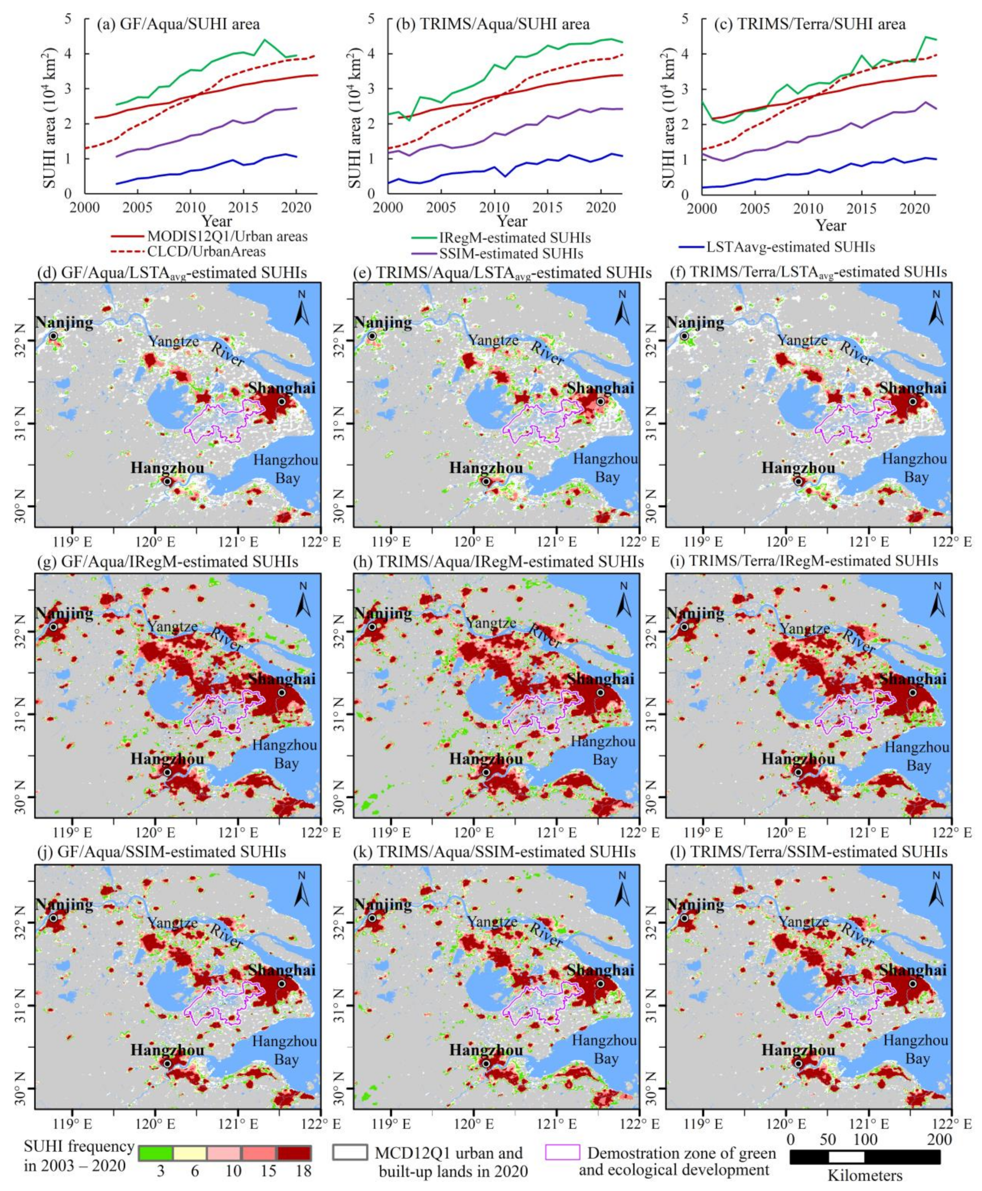
3.1. Temporal Variations in the Footprint of SUHIs in the YRDUA Region During 2000–2022

Each grid point classified as part of the SUHIs was identified on the basis that its LSTA annual cycle significantly resembled the urban reference LSTA annual cycle in terms of average values, variations, and shapes in the YRDUA region for each year in 2000–2022 (chi-square test, 0.05 significance level). Using the seven urban reference LSTA series generated from long-term mean LSTAs adopting K-means clustering with K = 2–8, the SUHI footprints were found to have consistent linear growth rates of 0.74–0.80 × 10⁴ km², 0.70–0.94 × 10⁴ km², and 0.82–0.87 × 10⁴ km² per decade for the GF Aqua, TRIMS Terra, and TRIMS Aqua datasets, respectively, in the same period of 2003–2020. Differences in the SUHI footprints between two adjacent urban reference LSTA series decreased from 1.0 × 10⁴ km² at K = 2–3 to 0.15 × 10⁴ km² at K = 4 and were lower than 0.03 × 10⁴ km² at K = 5–8 (Figure 3a–c). Barely urban grid points were wrongly excluded from the SUHIs within the urban reference areas at K >3 (Figure 3d–f). We selected the maximum SUHI footprint obtained from the urban reference LSTA with K = 4 in the K-means clustering as the optimal footprint for each year in 2000–2022 (purple lines in Figure 3d–f). These optimal SUHI footprints were cross-validated among the TRIMS Terra, TRIMS Aqua, and GF Aqua datasets for the same period of 2003–2020, showing the same linear growth rate of 0.80 × 10⁴ km² per decade and consistent ranges of approximately 1.06–2.39 × 10⁴ km², 1.09–2.44 × 10⁴ km², and 1.06–2.45 × 10⁴ km².

Importantly, the consistent footprints of the SUHIs derived from the TRIMS Terra, TRIMS Aqua, and GF Aqua datasets were far smaller than the corresponding urban sizes indicated by the MCD12Q1 and CLCD datasets at a 30% ISA threshold (Figure 4a), meaning that urban planners can enhance the transition zone surrounding the SSIM-estimated SUHI zone in urban areas to mitigate the adverse effects of SUHIs over the YRDUA region in future urban development.

3.2. Spatial Expansions of the SUHIs in the YRDUA Region During 2000–2022

Accurate spatial information on the transition zone between urban areas and the SUHI zone assists urban planners in developing strategies for mitigating SUHIs. The SSIM-based method captured similar spatial patterns and consistent footprints of the SUHIs from the GF Aqua, TRIMS Terra, and TRIMS Aqua datasets in the YRDUA region during the period of 2003–2020 (Figure 4). The SSIM-estimated SUHIs and the MCD12Q1 and CLCD urban areas showed linear growths of approximately 0.80 × 10⁴ km², 0.60 × 10⁴ km², and 1.30 × 10⁴ km² per decade, respectively (Figure 4a). In addition, the ratio of the SSIM-estimated SUHI footprint to the MCD12Q1 urban size increased notably from 43.0% in 2000 to 62.0% in 2022 (Figure 4b). After 2005, this ratio fluctuated approximately within the range of 54.5–68.2% relative to the CLCD urban size at a 30% ISA threshold (Figure 4c). Regional SUHIs had a spatial size larger than the CLCD high-density urban and built-up areas at a 50% ISA threshold (Figure 4a), and they experienced rapid expansion over mid-sized and large cities, with a footprint less than the urban size derived from the low-density to high-density MCD12Q1 and CLCD urban and built-up areas at a 30% ISA threshold (Figure 4d–f). Since the Chinese government implemented a development plan in 2016 to restrict the rapid expansion of large cities in the YRDUA region, the growth of SUHIs has shifted from large cities (e.g., Nanjing, Changzhou, Shanghai, and Hangzhou) along the Yangtze River and in Hangzhou Bay in 2003–2010 to small- and mid-sized cities in the middle and northern YRDUA after 2015.

Urban reference areas exhibiting a stable SUHI phenomenon had the highest yearly LSTA, exceeding 3 °C for the GF Aqua and TRIMS Aqua datasets and 2 °C for the TRIMS Terra dataset. The transition zone between the MCD12Q1 urban areas and the SUHI zone exhibited a relatively weak LSTA lower than 1.5 °C for the GF Aqua, TRIMS Aqua, and TRIMS Terra datasets (Figure 5a,c,e). Importantly, the ratio of the average SUHI footprint from the three LST data sources to the MCD12Q1 urban size increased monotonically from 0.43 to 0.62 because of rapid urbanization in 2000–2022 (Figure 4b), with there being a stable transition zone of approximately 1.2 × 10⁴ km² between the MCD12Q1 urban areas and SUHI zone, meaning that the YRDUA region experienced worsening SUHIs over low-density MCD12Q1 urban areas in 2000–2022 (Figure 5b,d,f).

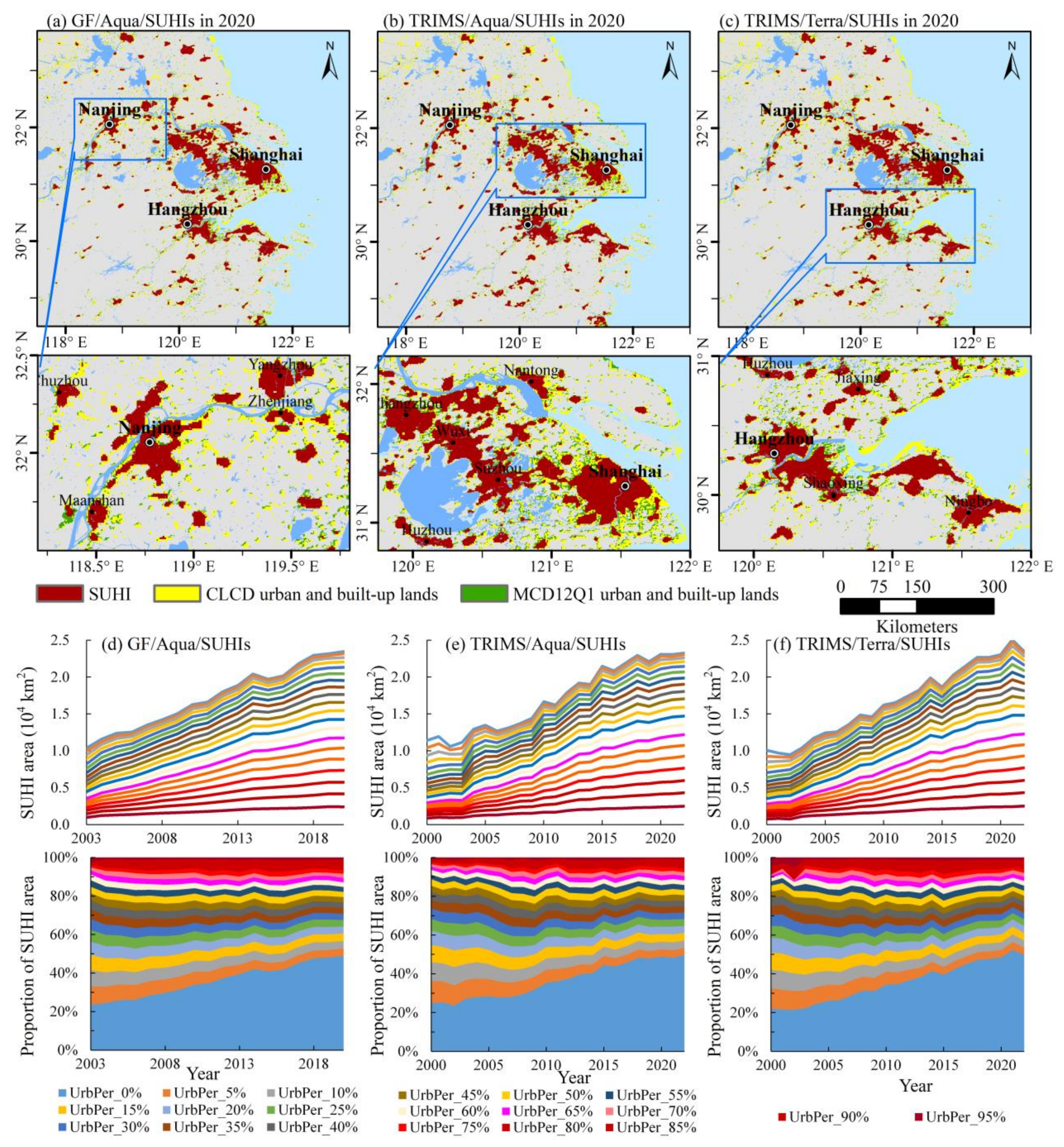
3.3. ISA Proportion Threshold of Urban and Built-Up Areas Related to a Stable SUHI Phenomenon

Ecological redline controls in urban and built-up areas should urgently be strengthened to prevent urban filling and clustering expansion in many urban agglomerations of China [65]. An ecological redline to limit the rapid expansion of high-density urban areas has been emphasized in urban development planning for the YRDUA region since 2016. We further investigated the ISA threshold of urban and built-up areas related to a stable SUHI phenomenon to identify the ecological redline control of high-density built-up areas in the YRDUA region. Following the 1 km × 1 km LST data, we identified urban and built-up areas with a continuous ISA density by applying a 1 km × 1 km sliding window to the 30 m × 30 m CLCD ISA data for 2000–2022.

Figure 6a–c show that the footprint of regional SUHIs was notably less than the spatial extent of urban and built-up areas derived from the CLCD and MCD12Q1 land cover data at a 30% ISA threshold. Here, using 20 ISA thresholds from 0% to 100% at 5% intervals, we identified the urban and built-up areas and assessed their relationship with the SUHIs according to the continuous density of the CLCD ISA data. The spatial extent of SUHIs expanded more rapidly within the mid- and low-density urban areas (ISA density below 60%) than within the high-density urban areas (ISA density above 60%) during 2000–2022 (lines in Figure 6d–f). The low-density CLCD urban areas experienced a growth rate of approximately 0.53–0.80 × 10⁴ km² per decade, whereas high-density urban areas grew more slowly at a rate of approximately 0.08–0.49 × 10⁴ km² per decade. Correspondingly, a stable SUHI proportion above 90% persisted within the high-density urban regions with an ISA density exceeding 65%, and urban areas with an ISA density below 60% exhibited a rapidly increasing tendency in SUHI proportion during the period of 2000–2022 (shading in Figure 6d–f). Therefore, the rapid expansion of SUHIs was mainly located within the mid- and low-density urban areas with an ISA density below 60%. Furthermore, no specific ISA threshold accurately captured the spatial size of regional SUHIs equal to the CLCD urban size in the YRDUA region during 2000–2022, mainly attributed to the strong fluctuations in the proportion of SUHIs within urban areas at a 25–60% ISA threshold, along with the high-density urban size being far less than the scale of the SUHIs (shading in Figure 6d–f). Given a stable SUHI proportion of approximately 90% within the high-density urban areas during 2000–2022, we recommend an ISA proportion of 65% as the ecological redline of urbanization to prevent the worsening of SUHIs in the YRDUA region.

3.4. Temporal Variations in SUHI Extent at Different SUHI Intensities in the SUHI Zone

The rapid expansion of SUHI footprints derived from the GF Aqua, TRIMS Aqua, and TRIMS Terra datasets mainly occurred in areas with moderate-to-high levels of yearly maximum and average SUHI intensities, with a severe SUHI intensity corresponding to a higher CLCD ISA density (Figure 6 and

Table 1. Linear tendencies in the spatial extent of SUHIs at different intensities and the CLCD urban areas during 2000–2022 (unit: 10⁴ km² per decade).

SUHI levels		Weak		Moderate		Severe
		2 °C	3 °C	4 °C	5 °C	6 °C	7 °C	8 °C	9 °C	10 °C
Maximum SUHI	GF/Aqua	–	−0.17	0.38	0.39	0.23	0.07	0.02	–	–
	TRIMS/Aqua	–	−0.15	0.08	0.28	0.25	0.15	0.08	–	–
	TRIMS/Terra	−0.18	0.29	0.4	0.21	0.05	0.01	–	–	–
SUHI levels		Weak			Moderate			Severe
		0.5 °C	1.0 °C	1.5 °C	2.0 °C	2.5 °C	3.0 °C	3.5 °C	4.0 °C	4.5 °C
Averaged SUHI	GF/Aqua	–	−0.14	−0.01	0.41	0.32	0.18	0.06	0.01	–
	TRIMS/Aqua	–	−0.13	−0.14	0.11	0.28	0.24	0.16	0.09	0.05
	TRIMS/Terra	−0.12	−0.16	0.43	0.34	0.17	0.06	0.01	–	–
CLCD/ISAlevels	Low density			Moderate density				High density
	10%	20%	30%	40%	50%	60%	70%	80%	90%	100%
Tendency	−0.58	−0.18	−0.02	0.04	0.09	0.10	0.13	0.15	0.15	0.15

Note: “–” represents no data.

). A weak SUHI intensity was observed in urban areas with a CLCD ISA density below 60%, whereas moderate and severe SUHI intensities corresponded to a high CLCD ISA density above 60% in 2000–2022. The spatial extent of areas experiencing moderate and severe intensities of the yearly maximum GF Aqua SUHI expanded rapidly, by approximately 0.23–0.39 × 10⁴ km² per decade; the spatial extent of areas experiencing moderate and severe intensities of the yearly maximum TRIMS Aqua SUHI increased linearly at approximately 0.15–0.28 × 10⁴ km² per decade; and the spatial extent of areas experiencing a moderate intensity of the yearly maximum TRIMS Terra SUHI had the highest linear increases of approximately 0.21–0.40 × 10⁴ km² per decade from 2000 to 2022.

Compared with the yearly maximum SUHI derived from the GF Aqua, TRIMS Aqua, and TRIMS Terra datasets, the yearly SUHI showed a faster spatial expansion of approximately 0.11–0.43 × 10⁴ km² per decade for the moderate type of SUHI, whereas the severe SUHI type exhibited a slower linear increase of 0.01–0.16 × 10⁴ km² per decade (Table 1). Except for the weak and severe types of the yearly maximum TRIMS Aqua SUHIs, all other SUHI types had a stable CLCD ISA density (the line graphs in Figure 7). In the SSIM-estimated SUHI zone, areas of a low CLCD ISA density showed a rapid decline of approximately −0.58 to −0.02 × 10⁴ km² per decade, whereas areas of moderate and high CLCD ISA densities showed notable expansion at a rate of approximately 0.04–0.15 × 10⁴ km² per decade. Urban planners and decision-makers should take effective measures to prevent the rapid expansion of moderate and severe SUHIs in moderate- and high-density urban areas in the YRDUA region.

4. Discussion

4.1. Advantages of the SSIM-Based Method in Quantifying Regional SUHIs

Setting the long-term mean LSTA to 1.0 °C as an intensity threshold to quantify SUHI footprints led to overestimations in the Shanghai metropolitan area and underestimations in the Nanjing and Hangzhou metropolitan areas (Figure 2b). Therefore, no single threshold can accurately capture the spatial patterns and footprints of regional SUHIs, given the large spatial differences in LSTA_avg over the YRDUA region. By applying a natural-break algorithm to classify the LSTA_avg, IRegM, and SSIM values into five categories for each year in 2000–2022, we defined the first category—characterized by the highest LSTA_avg and SSIM values and the lowest IRegM values—as the LSTA_avg-estimated, SSIM-estimated, and IRegM-estimated SUHI zones. This classification revealed diverse spatial patterns and footprints of the SUHIs in the YRDUA region during 2000–2022 (Figure 8). The LSTA_avg-based method, by ignoring spatial differences in the SUHI intensity, generated inconsistent spatial patterns in the Shanghai and Nanjing metropolitan areas and underestimated SUHI footprints as being approximately one-third of the MCD12Q1 urban size in the YRDUA region, as evidenced by the GF Aqua, TRIMS Aqua, and TRIMS Terra datasets (Figure 8a–f). Compared with the IRegM-estimated and SSIM-estimated SUHIs, the LSTA_avg-estimated SUHIs exhibited the slowest growth, expanding by approximately 0.39–0. 50 × 10⁴ km² per decade. Among the three methods, the IRegM-based method was sensitive to urbanization and the weather and climate conditions, resulting in the most inflated and fluctuating SUHI footprints exceeding the MCD12Q1 urban size in 2000–2022. This overestimation was due to the method not accounting for spatial differences in the annual averaged SUHI intensity within urban agglomerations (Figure 8g–i), resulting in a maximum linear increasing rate of approximately 1.02–1.15 × 10⁴ km² per decade across the GF Aqua, TRIMS Aqua, and TRIMS Terra data in 2000–2022. Given that the footprints of the IRegM-estimated SUHIs exceeded the MCD12Q1 urban size, urban planners have almost no chance of balancing the social and economic benefits of urbanization with worsening regional SUHIs in future urban planning.

The SSIM-based method effectively integrated the structural similarity of the LSTA annual cycle at each grid point with the urban reference LSTA annual cycle in terms of average values, variances, and shapes. This method yielded stable spatial patterns and consistent footprints of the SUHIs from the GF Aqua, TRIMS Aqua, and TRIMS Terra data, despite notable differences in LSTAs among the three LST data sources (Figure 1c and Figure 5a,c,e). In comparison with the IRegM-based and LSTA_avg-based methods, the SSIM-based method generated more reliable spatial patterns (Figure 8g–l) and yielded more reasonable footprints of regional SUHIs that were smaller than the urban size in the YRDUA region from 2000 to 2022. Hence, urban planners can enhance the transition zone between the SSIM-estimated SUHI zone and the MCD12Q1 urban areas to mitigate the adverse effects of SUHIs in future urban planning (Figure 8j–l).

4.2. Potential Implications of the SSIM-Estimated SUHIs in Urban Planning

Since 2016, urban development planning for the YRDUA has emphasized the need for an ecological redline to slow the expansion of high-density urban areas. In 2019, the Chinese government further established a demonstration zone of green and integrated ecological development to maximize the benefits of urbanization at the minimum cost of resources, the eco-environment, and the climate over the YRDUA region. This demonstration zone comprises the Qingpu district of Shanghai, the Wujiang district of Suzhou in Jiangsu province, and the Jiashan County in Zhejiang province, depicted by a purple polygon in Figure 8.

The LSTA_avg-based and IRegM-based methods yielded contradictory guidelines for urban planning. The weak LSTA_avg-estimated SUHIs in the demonstration zone suggest that reasonable urbanization can be encouraged, whereas the inflated IRegM-estimated SUHIs larger than the MCD12Q1 urban size suggest that rapid urbanization should be restricted. Figure 1b and Figure 2b,c show that the demonstration zone had a small spatial extent of SUHIs in 2000–2022. Correspondingly, the SSIM-based method yielded a spatial extent of SUHIs less than the MCD12Q1 urban size in this demonstration zone (Figure 8j–l). Hence, the SSIM-estimated SUHIs provide unambiguous guidance for urban planning in mitigating the adverse effects of SUHIs in this demonstration zone; that is, urban planners can restrict the excessive expansion of urban areas with an ISA density exceeding 65%, and they can enhance the transition zone between urban areas and the SSIM-estimated SUHI zone by reasonably allocating commercial, industrial, and other functional zones in future development.

4.3. Uncertainties of SSIM-Estimated SUHIs over Urban Agglomerations

The SSIM index of the annual cycles of LSTAs between urban and other land cover types was adopted to characterize the spatial patterns and footprints of regional SUHIs. This approach considers that several factors potentially affect the accuracy of SSIM-estimated SUHIs. Given its strong dependency on variations in the annual LSTA cycle between urban areas and other land cover types, the SSIM-based method is more effective for characterizing the SUHI during the day than at night. As shown in Figure 2 and Figure 3, the performance of the SSIM-based method in quantifying regional SUHIs depends on the selection of urban reference LSTA series. Seven urban reference LSTA series, derived from the long-term averaged LSTA from 2000 to 2022 by applying a K-means approach, corresponded to different SUHI footprints and can introduce uncertainty in the characterization of regional SUHIs. Moreover, uncertainties in SSIM-estimated SUHIs are linked with the accuracy of quantifying the LSTA related to urbanization using the RF algorithm together with climate, environmental, geographical, biophysical, and topographical parameters.

Fortunately, despite the strong effects of inter-annual variations in weather and climate and different LST data sources on SUHI intensities, the SSIM-based method generated stable spatial patterns and reasonable footprints of the SUHIs from three data sources in the YRDUA region during 2000–2022. This stability is attributed to the SSIM index accommodating the integrated contribution of the averaged values, variations, and shapes of all LSTA annual cycles within urban agglomerations.

5. Conclusions

Previous studies have reported inflated and varying SUHI spatial footprints of approximately 1.0–3.0 times the urban size from the 8-day composite daytime MODIS Aqua LST datasets in the metropolitans of Nanjing, Shanghai, and Hefei over the YRDUA region during 2003–2012 [22] and of approximately 42,328 km² and 38,884 km², being 1.58 and 2.0 times the urban size in the entire YRDUA region, from the 8-day composite MODIS Terra and Aqua LST datasets in 2015–2020 [21]. The varying and inflated footprints of SUHIs from different methods and LST datasets are not conducive to urban planners developing reasonable strategies to mitigate the SUHIs in future urban development. Our proposed solution classified each grid point as part of the SUHIs on the basis that its LSTA annual cycle significantly resembled the urban reference LSTA annual cycle in terms of average values, variations, and shapes, thereby yielding stable and reliable spatial patterns of the SUHIs. A clear transition zone within urban areas and cross-validated footprints of approximately 1.06–2.39 × 10⁴ km², 1.09–2.44 × 10⁴ km², and 1.06–2.45 × 10⁴ km² were obtained from among the TRIMS Terra, TRIMS Aqua, and GF Aqua datasets for the same period of 2003–2020, although significant differences in the seasonal or diurnal SUHI intensity were observed among the three LST datasets. The consistent footprints of the SUHIs derived from the TRIMS Terra, TRIMS Aqua, and GF Aqua datasets were far smaller than the corresponding urban sizes indicated by the MCD12Q1 and CLCD datasets at a 30% ISA threshold, meaning that urban planners can enhance the transition zone surrounding the SSIM-estimated SUHI zone in urban areas to mitigate the adverse effects of SUHIs over the YRDUA region in future urban design.

Given that all SUHIs derived from the TRIMS Terra, TRIMS Aqua, and GF Aqua LST datasets maintained a stable proportion of approximately 90% in high-density urban regions with an ISA above 65%, we recommend the 65% ISA threshold as an ecological redline control for the expansion of high-density urban areas to prevent the worsening of SUHIs in the YRDUA region. In 2019, the Chinese government established a demonstration zone to maximize the social and economic benefits at a minimum cost of resources, the environment, and the climate in the YRDUA region. The SSIM-estimated SUHIs exhibited a spatial extent smaller than the urban size, providing clear guidance for urban planning to mitigate SUHI-related adverse effects in this demonstration zone; that is, urban planners can restrict the excessive expansion of urban areas with an ISA density exceeding 65%, and they can enhance the transition zone between urban areas and the SSIM-estimated SUHI zone by reasonably allocating commercial, industrial, and other functional zones in future development. Considering that urban areas rapidly transformed into SUHIs, with the ratio of the SUHI extent to the urban size increasing from 0.43 to 0.62 during 2000–2022, urban planners should also take measures to prevent the rapid expansion of high-density urban areas. In summary, this study provides a practicable solution for decision-makers and urban planners to systematically understand the spatiotemporal variations in regional SUHIs and search for cross-validated urban spatial patterns and scales from multiple data sources to guide future urban development.

References

1. Voogt, J.A.; Oke, T.R. Thermal remote sensing of urban climates. Remote Sens. Environ. 2003, 86, 370–384. [Google Scholar] [CrossRef]
2. Manoli, G.; Fatichi, S.; Schläpfer, M.; Yu, K.L.; Crowther, T.W.; Meili, N.; Burlando, P.; Katul, G.G.; Bou-Zeid, E. Magnitude of urban heat islands largely explained by climate and population. Nature 2019, 573, 55–60. [Google Scholar] [CrossRef] [PubMed]
3. Oke, T.R.; Mills, G.; Christen, A.; Voogt, J.A. Urban Climates; Cambridge University Press: Cambridge, UK, 2017. [Google Scholar] [CrossRef]
4. Stewart, I.D.; Krayenhoff, E.S.; Voogt, J.A.; Lachapelle, J.A.; Broadbent, A.M. Time evolution of the surface urban heat island. Earths Future 2021, 9, e2021EF002178. [Google Scholar] [CrossRef]
5. Hu, J.; Yang, Y.B.; Zhou, Y.Y.; Zhang, T.; Ma, Z.F.; Meng, X.J. Spatial patterns and temporal variations of footprint and intensity of surface urban heat island in 141 China cities. Sustain. Cities Soc. 2022, 77, 103585. [Google Scholar] [CrossRef]
6. Venter, Z.S.; Chakraborty, T.; Lee, X.H. Crowdsourced air temperatures contrast satellite measures of the urban heat island and its mechanisms. Sci. Adv. 2021, 7, eabb9569. [Google Scholar] [CrossRef]
7. Li, X.M.; Asrar, G.R.; Imhoff, M.; Li, X.C. The surface urban heat island response to urban expansion: A panel analysis for the conterminous United States. Sci. Total Environ. 2017, 605, 426–435. [Google Scholar] [CrossRef]
8. Zhou, X.F.; Chen, H. Impact of urbanization-related land use land cover changes and urban morphology changes on the urban heat island phenomenon. Sci. Total Environ. 2018, 635, 1467–1476. [Google Scholar] [CrossRef]
9. Lyu, H.; Wang, W.; Zhang, K.E.; Cao, C.; Xiao, W.; Lee, X.H. Factors influencing the spatial variability of air temperature urban heat island intensity in Chinese cities. Adv. Atmos. Sci. 2024, 41, 817–829. [Google Scholar] [CrossRef]
10. Mathivanan, M.; Duraisekaran, E. Identification and quantification of localized urban heat island intensity and footprint for Chennai Metropolitan Area during 1988–2023. Environ. Monit. Assess. 2025, 197, 91. [Google Scholar] [CrossRef]
11. United Nations, Department of Economic and Social Affairs, Population Division. World Urbanization Prospects: The 2018 Revision; United Nations: New York, NY, USA, 2019; Available online: https://www.un.org/development/desa/pd/sites/www.un.org.development.desa.pd/files/files/documents/2020/Feb/un_2018_wup_highlights.pdf (accessed on 1 February 2025).
12. Fang, C.L.; Yu, D.L. Urban agglomeration: An evolving concept of an emerging phenomenon. Landsc. Urban Plan. 2017, 162, 126–136. [Google Scholar] [CrossRef]
13. Geng, S.B.; Yang, L.; Sun, Z.Y.; Wang, Z.H.; Qian, J.X.; Jiang, C.; Wen, M.L. Spatiotemporal patterns and driving forces of remotely sensed urban agglomeration heat islands in South China. Sci. Total Environ. 2021, 800, 149499. [Google Scholar] [CrossRef] [PubMed]
14. Wang, Z.A.; Meng, Q.Y.; Allam, M.; Hu, D.; Zhang, L.L.; Menenti, M. Environmental and anthropogenic drivers of surface urban heat island intensity: A case-study in the Yangtze River Delta, China. Ecol. Indic. 2021, 128, 107845. [Google Scholar] [CrossRef]
15. Wu, Z.F.; Xu, Y.; Cao, Z.; Yang, J.X.; Zhu, H. Impact of urban agglomeration and physical and socioeconomic factors on surface urban heat islands in the Pearl River Delta Region, China. IEEE J. Sel. Top. Appl. Earth Obs. Remote Sens. 2021, 14, 8815–8822. [Google Scholar] [CrossRef]
16. Fu, X.C.; Yao, L.; Xu, W.T.; Wang, Y.X.; Sun, S. Exploring the multi-temporal surface urban heat island effect and its driving relation in the Beijing-Tianjin-Hebei urban agglomeration. Appl. Geogr. 2022, 144, 102714. [Google Scholar] [CrossRef]
17. Peng, J.; Qiao, R.L.; Wang, Q.; Yu, S.Y.; Dong, J.Q.; Yang, Z.W. Diversified evolutionary patterns of surface urban heat island in new expansion areas of 31 Chinese cities. Npj Urban Sustain. 2024, 4, 14. [Google Scholar] [CrossRef]
18. Ren, J.Y.; Yang, J.; Yu, W.B.; Cong, N.; Xiao, X.M.; Xia, J.H.; Li, X.M. Spatiotemporal evolution of surface urban heat islands: Concerns regarding summer heat wave periods. J. Geogr. Sci. 2024, 34, 1065–1082. [Google Scholar] [CrossRef]
19. Zhang, H.; Cen, X.H.; An, H.; Yin, Y.X. Quantitative assessment and driving factors analysis of surface urban heat island of urban agglomerations in China based on GEE. Environ. Sci. Pollut. Res. 2024, 31, 47350–47364. [Google Scholar] [CrossRef]
20. Xie, Z.Q.; Du, Y.; Miao, Q.; Zhang, L.L.; Wang, N. An approach to characterizing the spatial pattern and scale of regional heat islands over urban agglomerations. Geophys. Res. Lett. 2022, 49, e2022GL099117. [Google Scholar] [CrossRef]
21. Du, Y.; Xie, Z.Q.; Zhang, L.L.; Wang, N.; Wang, M.; Hu, J.W. Machine-learning-assisted characterization of regional heat islands with a spatial extent larger than the urban size. Remote Sens. 2024, 16, 599. [Google Scholar] [CrossRef]
22. Zhou, D.C.; Zhao, S.Q.; Zhang, L.X.; Sun, G.; Liu, Y.Q. The footprint of urban heat island effect in China. Sci. Rep. 2015, 5, 11160. [Google Scholar] [CrossRef]
23. Si, M.; Li, Z.L.; Nerry, F.; Tang, B.H.; Leng, P.; Wu, H.; Zhang, X.; Shang, G. Spatiotemporal pattern and long-term trend of global surface urban heat islands characterized by dynamic urban-extent method and MODIS data. ISPRS J. Photogramm. 2022, 183, 321–335. [Google Scholar] [CrossRef]
24. Wang, R.; Voogt, J.; Ren, C.; Ng, E. Spatial-temporal variations of surface urban heat island: An application of local climate zone into large Chinese cities. Build. Environ. 2022, 222, 109378. [Google Scholar] [CrossRef]
25. Martin, P.; Baudouin, Y.; Gachon, P. An alternative method to characterize the surface urban heat island. Int. J. Biometeorol. 2015, 59, 849–861. [Google Scholar] [CrossRef] [PubMed]
26. Liu, Y.H.; Fang, X.Y.; Xu, Y.M.; Zhang, S.; Luan, Q.Z. Assessment of surface urban heat island across China’s three main urban agglomerations. Theor. Appl. Climatol. 2018, 133, 473–488. [Google Scholar] [CrossRef]
27. Sun, Y.W.; Gao, C.; Li, J.L.; Wang, R.; Liu, J. Evaluating urban heat island intensity and its associated determinants of towns and cities continuum in the Yangtze River Delta urban agglomerations. Sustain. Cities Soc. 2019, 50, 101659. [Google Scholar] [CrossRef]
28. Liu, H.M.; Huang, B.; Zhan, Q.M.; Gao, S.H.; Li, R.R.; Fan, Z.Y. The influence of urban form on surface urban heat island and its planning implications: Evidence from 1288 urban clusters in China. Sustain. Cities Soci. 2021, 71, 102987. [Google Scholar] [CrossRef]
29. Hsu, A.; Sheriff, G.; Chakraborty, T.; Manya, D. Disproportionate exposure to urban heat island intensity across major US cities. Nat. Commun. 2021, 12, 2721. [Google Scholar] [CrossRef]
30. Yao, R.; Huang, X.; Zhang, Y.J.; Wang, L.C.; Li, J.Y.; Yang, Q.Q. Estimation of the surface urban heat island intensity across 1031 global cities using the regression-modification-estimation (RME) method. J. Clean. Prod. 2024, 434, 140231. [Google Scholar] [CrossRef]
31. Li, Y.F.; Schubert, S.; Kropp, J.P.; Rybski, D. On the influence of density and morphology on the Urban Heat Island intensity. Nat. Commun. 2020, 11, 2647. [Google Scholar] [CrossRef]
32. Acosta, M.P.; Vahdatikhaki, F.; Santos, J.; Hammad, A.; Dor′ee, A.G. How to bring UHI to the urban planning table? A data-driven modeling approach. Sustain. Cities Soc. 2021, 71, 102948. [Google Scholar] [CrossRef]
33. Yang, Q.Q.; Xu, Y.; Tong, X.H.; Huang, X.; Liu, Y.; Chakraborty, T.C.; Xia, C.J.; Hu, T. An adaptive synchronous extraction (ASE) method for estimating intensity and footprint of surface urban heat islands: A case study of 254 North American cities. Remote Sens. Environ. 2023, 297, 113777. [Google Scholar] [CrossRef]
34. Yao, R.; Wang, L.C.; Huang, X.; Niu, Y.; Chen, Y.S.; Niu, Z.G. The influence of different data and methods on estimating the surface urban heat island intensity. Ecol. Indic. 2018, 89, 45–55. [Google Scholar] [CrossRef]
35. Hou, H.; Estoque, R.C. Detecting cooling effect of landscape from composition and configuration: An urban heat island study on Hangzhou. Urban For. Urban Gree. 2020, 53, 126719. [Google Scholar] [CrossRef]
36. Soydan, O. Effects of landscape composition and patterns on land surface temperature: Urban heat island case study for Nigde, Turkey. Urban Clim. 2020, 34, 100688. [Google Scholar] [CrossRef]
37. Wang, Q.; Wang, X.N.; Zhou, Y.; Liu, D.Y.; Wang, H.T. The dominant factors and influence of urban characteristics on land surface temperature using random forest algorithm. Sustain. Cities Soc. 2022, 79, 103722. [Google Scholar] [CrossRef]
38. Xiang, Y.; Ye, Y.; Peng, C.C.; Teng, M.J.; Zhou, Z.X. Seasonal variations for combined effects of landscape metrics on land surface temperature (LST) and aerosol optical depth (AOD). Ecol. Indic. 2022, 138, 108810. [Google Scholar] [CrossRef]
39. Ezimand, K.; Azadbakht, M.; Aghighi, H. Analyzing the effects of 2D and 3D urban structures on LST changes using remotely sensed data. Sustain. Cities Soci. 2021, 74, 103216. [Google Scholar] [CrossRef]
40. Taripanah, F.; Ranjbar, A. Quantitative analysis of spatial distribution of land surface temperature (LST) in relation ecohydrological, terrain and socio-economic factors based on Landsat data in mountainous area. Adv. Space Res. 2021, 68, 3622–3640. [Google Scholar] [CrossRef]
41. Yang, J.; Huang, X. The 30 m annual land cover dataset and its dynamics in China from 1990 to 2019. Earth Syst. Sci. Data 2021, 13, 3907–3925. [Google Scholar] [CrossRef]
42. Zhao, M.; Cheng, C.X.; Zhou, Y.Y.; Li, X.C.; Shen, S.; Song, C.Q. A global dataset of annual urban extents (1992–2020) from harmonized nighttime lights. Earth Syst. Sci. Data 2022, 14, 517–534. [Google Scholar] [CrossRef]
43. Somvanshi, S.S.; Kumari, M.; Sharma, R. Spatio-temporal analysis of rural-urban transitions and transformations in Gautam Buddha Nagar, India. Int. J. Environ. Sci. Technol. 2024, 21, 5079–5088. [Google Scholar] [CrossRef]
44. Adilkhanova, I.; Ngarambe, J.; Yun, G.Y. Recent advances in black box and white-box models for urban heat island prediction: Implications of fusing the two methods. Renew. Sust. Energ. Rev. 2022, 165, 112520. [Google Scholar] [CrossRef]
45. Yang, Q.Q.; Huang, X.; Tang, Q.H. The footprint of urban heat island effect in 302 Chinese cities: Temporal trends and associated factors. Sci. Total Environ. 2019, 655, 652–662. [Google Scholar] [CrossRef] [PubMed]
46. Shen, P.K.; Zhao, S.Q. Intensifying urban imprint on land surface warming: Insights from local to global scale. iScience 2024, 27, 109110. [Google Scholar] [CrossRef]
47. Yu, Z.W.; Yao, Y.W.; Yang, G.Y.; Wang, X.R.; Vejre, H. Spatiotemporal patterns and characteristics of remotely sensed region heat islands during the rapid urbanization (1995–2015) of southern China. Sci. Total Environ. 2019, 674, 242–254. [Google Scholar] [CrossRef]
48. Hou, L.; Yue, W.Z.; Liu, X. Spatiotemporal patterns and drivers of summer heat island in Beijing-Tianjin-Hebei Urban Agglomeration, China. IEEE J. Sel. Top. Appl. Earth Obs. Remote Sens. 2021, 14, 7516–7527. [Google Scholar] [CrossRef]
49. Yao, L.; Sun, S.; Song, C.Y.; Li, J.; Xu, W.T.; Xu, Y. Understanding the spatiotemporal pattern of the urban heat island footprint in the context of urbanization, a case study in Beijing, China. Appl. Geogr. 2021, 133, 102496. [Google Scholar] [CrossRef]
50. Han, J.; Mo, N.; Cai, J.Y.; Ouyang, L.X.; Liu, Z.X. Advancing the local climate zones framework: A critical review of methodological progress, persisting challenges, and future research prospects. Hum. Soc. Sci. Commun. 2024, 11, 538. [Google Scholar] [CrossRef]
51. Stewart, I.D.; Oke, T.R. Local Climate Zones for Urban Temperature Studies. Bull. Am. Meteorol. Soc. 2012, 93, 1879–1900. [Google Scholar] [CrossRef]
52. Bechtel, B.; Demuzere, M.; Mills, G.; Zhan, W.F.; Sismanidis, P.; Small, C.; Voogt, J. SUHI analysis using local climate zones—A comparison of 50 cities. Urban Clim. 2019, 28, 100451. [Google Scholar] [CrossRef]
53. Demuzere, M.; Kittner, J.; Martilli, A.; Mills, G.; Moede, C.; Stewart, I.D.; van Vliet, J.; Bechtel, B. A global map of local climate zones to support earth system modeling and urban-scale environmental science. Earth Syst. Sci. Data 2022, 14, 3835–3873. [Google Scholar] [CrossRef]
54. Rahmani, N.; Sharifi, A. Urban heat dynamics in Local Climate Zones (LCZs): A systematic review. Build. Environ. 2025, 267, 112225. [Google Scholar] [CrossRef]
55. Mohammad, P.; Goswami, A.; Chauhan, S.; Nayak, S. Machine learning algorithm based prediction of land use land cover and land surface temperature changes to characterize the surface urban heat island phenomena over Ahmedabad city, India. Urban Clim. 2022, 42, 101116. [Google Scholar] [CrossRef]
56. Wang, Z.; Bovik, A.C.; Sheikh, H.R.; Simoncelli, E.P. Image quality assessment: From error visibility to structural similarity. IEEE Trans. Image Process. 2004, 13, 600–611. [Google Scholar] [CrossRef]
57. Jia, A.L.; Liang, S.L.; Wang, D.D.; Malick, K.; Zhou, S.G.; Hu, T.; Xu, S. Advances in methodology and generation of all-weather land surface temperature products from polar-orbiting and geostationary satellites: A comprehensive review. IEEE Geosci. Remote Sens. Mag. 2024, 12, 218–260. [Google Scholar] [CrossRef]
58. Zhang, T.; Zhou, Y.Y.; Zhu, Z.Y.; Li, X.M.; Asrar, G.R. A global seamless 1 km resolution daily land surface temperature dataset (2003–2020). Earth Syst. Sci. Data 2022, 14, 651–664. [Google Scholar] [CrossRef]
59. Tang, W.B.; Zhou, J.; Ma, J.; Wang, Z.W.; Ding, L.R.; Zhang, X.D.; Zhang, X. TRIMS LST: A daily 1 km all-weather land surface temperature dataset for China’s landmass and surrounding areas (2000–2022). Earth Syst. Sci. Data 2024, 16, 387–419. [Google Scholar] [CrossRef]
60. Abercrombie, S.P.; Friedl, M.A. Improving the consistency of multitemporal land cover maps using a hidden Markov model. IEEE Trans. Geosci. Remote Sens. 2016, 54, 703–713. [Google Scholar] [CrossRef]
61. Liang, S.L.; Cheng, C.; Jia, K.; Jiang, B.; Liu, Q.; Xiao, Z.Q.; Yao, Y.J.; Yuan, W.; Zhang, X.T.; Zhao, X.; et al. The Global Land Surface Satellite (GLASS) products suite. Bull. Am. Meteorol. Soc. 2021, 102, E323. [Google Scholar] [CrossRef]
62. Amatulli, G.; Domisch, S.; Tuanmu, M.N.; Parmentier, B.; Ranipeta, A.; Malczyk, J.; Jetz, W. A suite of global, cross-scale topographic variables for environmental and biodiversity modeling. Sci. Data 2018, 5, 180040. [Google Scholar] [CrossRef]
63. Breiman, L. Random forests. Mach. Learn. 2001, 45, 5–32. [Google Scholar] [CrossRef]
64. Scholkmann, F.; Boss, J.; Wolf, M. An efficient algorithm for automatic peak detection in noisy periodic and quasi-periodic signals. Algorithms 2012, 5, 588–603. [Google Scholar] [CrossRef]
65. Kuang, W.H. Mapping global impervious surface area and green space within urban environments. Sci. China Earth Sci. 2019, 62, 1591–1606. [Google Scholar] [CrossRef]
Figure 1. Spatial distribution of the five dominant land use types from the MCD12Q1 data in 2022 (a); the TRIMS Aqua LSTA on days 255 and 25, 2022 (b,c); and the LSTA annual cycles of forests, cropland, towns, and middle and large cities in 2000–2022 (d).
Remotesensing 17 00892 g001
Figure 2. Urban areas from the MCD12Q1 land cover data in 2003, 2013, and 2022 (a); the long-term averaged LSTA in 2000–2022 (b); the LSTAavg-estimated SUHI zones by applying a K-Means clustering method at K = 2–8 (c); the LSTA linear increments from the GF Aqua, TRIMS Aqua, and TRIMS Terra LSTA datasets in 2003–2020 (df); and SSIM-estimated SUHI zone from the urban reference LSTA series of large cities (d) and the high averaged LSTA zone (gi).
Remotesensing 17 00892 g002
Figure 3. Variations in the SSIM-estimated SUHI footprints using the LSTA data of large cities and the high averaged LSTA zones classified by a K-Means clustering method at K = 2–8 (ac) and the non-SUHIs within the urban reference areas (df) for the GF Aqua, TRIMS Aqua, and TRIMS Terra datasets during 2000–2022.
Remotesensing 17 00892 g003
Figure 4. Temporal variations in the urban areas from the MCD12Q1 and CLCD datasets and the SUHI areas from the GF Aqua and TRIMS Aqua and Terra datasets (a); the proportion of SUHIs within the MCD12Q1 (b) and CLCD (c) urban areas; and the spatial footprints of regional SUHIs from the GF Aqua (d), TRIMS Aqua (e), and TRIMS Terra (f) datasets in the period 2003–2020.
Remotesensing 17 00892 g004
Figure 5. Temporal variations in the yearly LSTA related to urbanization (a,c,e) and the area of regional SUHIs from the GF Aqua, TRIMS Aqua, and TRIMS Terra datasets, and the transition zones (b,d,f) between the urban reference areas and MCD12Q1 urban areas and the SUHI zone during 2000–2022.
Remotesensing 17 00892 g005
Figure 6. Spatial distribution of the regional SUHIs from the GF Aqua, TRIMS Aqua, and TRIMS Terra datasets and the MCD12Q1 and CLCD urban areas at a 30% ISA threshold in 2020 (ac), and temporal variations in the ratio of SUHI area to CLCD urban area at an ISA threshold within 0–95% during 2000–2022 (df).
Remotesensing 17 00892 g006
Figure 7. Temporal variations in the spatial scale of yearly maximum (ac) and averaged (df) SUHIs at different intensities for the GF Aqua, TRIMS Aqua, and TRIMS Terra datasets during 2000–2022.
Remotesensing 17 00892 g007
Figure 8. Temporal variations in (ac) and spatial distributions of (dl) the SUHI footprint generated from the GF Aqua, TRIMS Aqua, and TRIMS Terra datasets by applying the LSTAavg, IRegM, and SSIM methods in the middle YRDUA region during 2000–2022.
Remotesensing 17 00892 g008