Influences of Global Warming and Upwelling on the Acidification in the Beaufort Sea

Abstract

Over the past three decades, increasing atmospheric CO₂ (AtmCO₂) has led to climate warming, sea ice reduction and ocean acidification in the Beaufort Sea (BS). Additionally, the effects of upwelling on the carbon cycle and acidification in the BS are still unknown. The Regional Arctic System Model (RASM) adequately reflects the observed long-term trends and interannual variations in summer sea ice concentration (SIC), temperature, partial pressure of CO₂ (pCO₂) and pH from 1990 to 2020. Multiple linear regression results from a control case show that surface (0–20 m) pH decline is significantly driven by AtmCO₂ and SIC, while AtmCO₂ dominates in subsurface (20–50 m) and deep layers (50–120 m). Regression results from a sensitivity case show that even if the AtmCO₂ concentration remained at 1990 levels, the pH would still exhibit a long-term decline trend, being significantly driven by SIC only in the surface layers and by SIC and net primary production (NPP) in the subsurface layers. In contrast to the nearly linearly increasing AtmCO₂ over the last three decades, the ocean pH shows more interannual variations that are significantly affected by SIC and mixed layer depth (MLD) in the surface, NPP and Ekman pumping velocity (EPV) in the subsurface and EPV only in the deep layer. The comparison of results from high and low SIC years reveals that areas with notable pH differences are overlapping regions with the largest differences in both SIC and MLD, and both cause a statistically significant increase in pCO₂ and decrease in pH. Comparison of results from high and low EPV years reveals that although stronger upwelling can lift up more nutrient-rich seawater in the subsurface and deep layers and lead to higher NPP and pH, this effect is more than offset by the higher DIC lifted up from deep water, leading to generally lower pH in most regions.

1. Introduction

As a result of fossil fuel emissions, atmospheric CO₂ (AtmCO₂) concentrations rose from 318 ppm in 1860 to 417 ppm in 2022, significantly exceeding historical normal levels [1]. As the Earth’s most important “carbon sink”, the ocean has absorbed 26% of the CO₂ emitted by humans [1,2,3]. The ocean has absorbed excess anthropogenic CO₂ from the atmosphere, leading to a sharp decline in parameters such as seawater pH (total scale pH (pH_T = −lg[H⁺]_T)), CO₃²⁻ concentration, and calcium carbonate saturation (Ω) [4,5,6]. This process of increasing the acidity of seawater is called ocean acidification [7].

The Arctic Ocean, due to its unique environment and characteristics, is highly sensitive to climate change responses and feedbacks [8], and is known as a bellwether of climate change. Although the Arctic Ocean covers only 4% of the global ocean area, it accounts for 5% to 14% of the total global ocean carbon uptake, and its acidification is particularly severe, with the seawater pH having decreased by approximately 0.2 over the past thirty years [9,10,11]. Seawater pH is highly sensitive to atmosphere–ice–ocean forcing and feedback, as well as to ecosystem shifts. Over the past thirty years, the ecological environment in the Arctic region has undergone rapid changes. For example, rising temperatures [12], significant sea ice melt [13], CO₂ exchange between the ocean and atmosphere [14,15], increased primary productivity [16,17], deepening of the marine mixed layer [17], and the occurrence of upwelling events [18,19,20] have all contributed to both long-term trends and interannual variations in acidification. Ocean acidification could significantly affect calcifying marine organisms and biogeochemical cycles in the diverse communities of high-latitude regions [21,22,23,24]. Therefore, it is necessary to enhance research and monitoring of ocean acidification in polar seas.

The acidification rate of the middle and low latitude oceans and the Southern Ocean is generally consistent with the rate predicted by increasing AtmCO₂ concentrations [10,25]. However, the rate of seawater acidification in the western Arctic Ocean is much faster than in other oceans [11]. Numerous studies suggest that the rapid acidification of the Arctic Ocean is mainly driven by rising AtmCO₂ levels and sea ice melting [11,26,27]. Rising temperatures lead to sea ice reduction, exposing low pCO₂ seawater to the atmosphere, which accelerates anthropogenic CO₂ uptake and lowers pH [4,28]. The acidification trend in the Canadian Basin (CB) shows a faster decline than that driven solely by AtmCO₂, whereas it is not the case in the Chukchi Sea, a marginal sea of the Arctic Ocean. The long-term acidification rate in the Chukchi Sea is relatively slower than in the CB, likely due to an increase in nutrient input from the Pacific Ocean, which enhances net primary productivity (NPP) and counterbalances the impact of elevated AtmCO₂ invasion [11,17]. As one of the marginal seas of the Arctic Ocean, the Beaufort Sea (BS) has a north–south continental slope. Under the influence of the Beaufort High and the Aleutian Low, prevailing easterly winds favor the generation of upwelling [29,30]. With the rapid retreat of summer sea ice in the BS, upwelling transports nutrient-rich water from the deep to the surface, enhancing NPP [20,31]. An increase in NPP caused by upwelling could potentially lead to a decrease in pCO₂ and an increase in pH. However, research has shown that during BS upwelling events, DIC-rich seawater is lifted to the surface, leading to an abnormal increase in surface pCO₂ [19,20]. This physical process caused by upwelling briefly converts the BS from a carbon sink to a carbon source, thus enhancing ocean acidification [32,33]. Furthermore, the mixed layer depth (MLD), driven by seasonal sea ice melting and winds, may also influence the carbonate system to some extent [34]. The influence of variations in Ekman pumping velocity (EPV, upwelling index), NPP, and MLD on the long-term trends and interannual variations in summer pH in the BS and the relative contributions of different factors (such as AtmCO₂ and SIC) remain uncertain.

Due to the uneven spatial and temporal distribution of observational data, previous studies have primarily focused on the acidification in the BS based on a limited number of cruises [14,19,20,32,33]. There is a dearth of studies on long-term spatiotemporal changes in pH across the entire region. Consequently, to address the limited observational data and the gaps in existing research, this study combines an ice–ocean physical and ecological coupling model [35] to analyze and comprehend the effects of AtmCO₂ concentration, SIC, EPV, NPP, and MLD on BS pH variations. The main focus of this study is the long-term trends and interannual variations in summer (June–September) pH in the BS from 1990 to 2020. The remote sensing SIC data and in situ observational data used to verify the Regional Arctic System Model (RASM) results are taken from the same period. Considering that pH variations are affected by intricate ice–ocean–ecosystem interactions, a multiple linear regression approach using RASM control and sensitivity experiments is conducted to examine the impact of different factors on BS pH, and quantify the relative contributions of each factor to pH changes. Additionally, by comparing five high and five low SIC years, we explore the impact of sea ice reduction on surface pH. We also examine the vertical influence of upwelling on pH by analyzing five high and five low EPV years. The rest of this paper is structured as follows: Section 2 covers the data and methods; Section 3 presents model validation, long-term trends of changes, interannual variations in pH, and the acidification mechanisms in the BS; Section 4 offers the discussion; Section 5 is the conclusions.

2. Materials and Methods

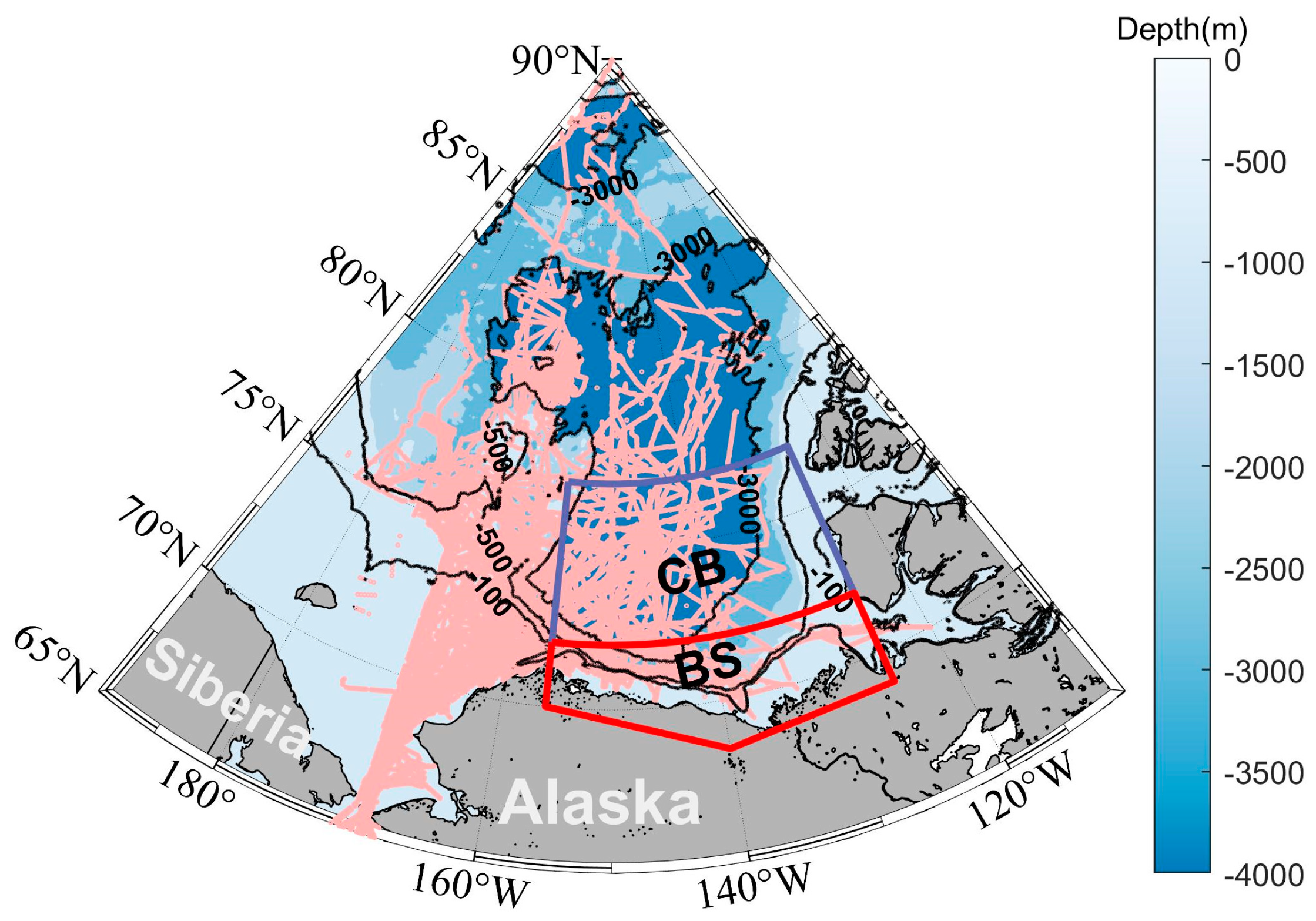
2.1. The RASM and Study Area

The RASM is a high-resolution ice–ocean physical and ecological coupling model with a horizontal resolution of 1/12° (approximately 9 km). It covers the region north of 30°N in the Northern Hemisphere, including sea ice in the Northern Hemisphere, Arctic land drainage, and major inflow and outflow pathways [35]. RASM is based on the Community Earth System Model (CESM) framework and comprises the Parallel Ocean Program version 2 (POP2) and Community Ice CodE (CICE) sea ice models, developed by the Los Alamos National Laboratory (LANL). The RASM enhances the ability to simulate key physical processes, feedback, and their impact on the Arctic climate system, while reducing uncertainties in predictions [36]. The initial conditions for temperature and salinity come from the Polar Science Center Hydrographic Climatology (PHC), while nitrate data are sourced from the gridded World Ocean Atlas (WOA2013) available on the National Oceanic and Atmospheric Administration (NOAA) website [37]. JRA-55 was used as the atmospheric forcing field [38]. The main component of the marine biogeochemistry (BGC) model is a moderately complex Nutrients–Phytoplankton–Zooplankton–Detritus (NPZD) model, which includes 26 state variables for phytoplankton, nutrients, zooplankton, and other carbon and nutrient pools [39]. In this study, we used model outputs from the summers (June–September) of 1990–2020. The variables included AtmCO₂, temperature, salinity, pH, pCO₂, dissolved inorganic carbon (DIC), SIC, the proportion of ice-free days (IFR, calculated as SIC < 10%), MLD, and NPP, where NPP refers to the total net primary productivity of three phytoplankton groups (diatoms, small phytoplankton, and diazotrophs) [31]. Two RASM experiment cases are set up as follows: (1) control case C uses observed AtmCO₂ concentration and (2) sensitivity experiment case S differs only in that it uses 1990 AtmCO₂ concentration for all the years from 1990 to 2020. Comparisons of those two cases are used to represent the effect of increasing AtmCO₂ concentration on BS acidification.

The Western Arctic Ocean ranges from 65 to 90°N and 175°E to 120°W (Figure 1). The BS and the CB are separated by the 72°N latitude [28]. The BS region spans from 68°N to 72°N and 120°E to 156°E; the CB region spans from 72°N to 77°N and 120°E to 156°E. This study mainly focuses on the BS region, a marginal sea with a north–south landward slope in the Western Arctic Ocean.

2.2. NSIDC Sea Ice Data, In Situ Observations and JRA-55 Reanalysis Data

The SIC dataset from NSIDC (https://nsidc.org/data/nsidc-0051/versions/2, accessed on 15 July 2023) is derived from passive microwave remote sensing calibration using three sensors: Nimbus-7 SMMR, SSM/Is, and SSMIS, with a spatial resolution of 25 × 25 km [40]. This study uses daily SIC data for the Arctic region from 1990 to 2020 for RASM validation.

The in situ surface observational data were obtained from international shared databases Mendeley Data (https://data.mendeley.com/datasets/2ccwgyf6cw/3, accessed on 5 March 2024) [11]. The data cover sea surface temperature, salinity, pCO₂, and pH from July to October of 1994 to 2020, with over 372,000 data entries, respectively. The water column observations were downloaded from the GLODAP database (https://glodap.info/index.php/data-access/, accessed on 3 June 2024) [41,42]. These sea surface and water column observational data are primarily used for validating the RASM.

The atmospheric reanalysis data JRA-55 (1958 to present) are used to drive the RASM (http://search.diasjp.net/en/dataset/JRA55, accessed on 13 September 2023), with a temporal resolution of 3 h and a spatial resolution of 0.5° [43]. The monthly average values of near-surface wind speed at 10 m from the JRA-55 reanalysis data are used to calculate EPV (see Section 2.3).

2.3. EPV and Multiple Linear Regression Calculations

In the complex environment with partial sea ice coverage, to calculate the strength index of EPV, it is necessary to consider not only the influence of atmosphere–seawater stress, but also the influence of sea ice–seawater stress [44], and the EPV is as follows [45]:

$$EPV={\displaystyle \frac{1}{\rho f}}\left(\nabla \times \overrightarrow{\tau }\right)$$

(1)

where $\overrightarrow{\tau }$ is the total surface stress (N/m²), ρ is the seawater density (Kg/m³), f is the Coriolis coefficient (s⁻¹), and $\overrightarrow{\tau }=\left(1-\alpha \right)\overrightarrow{{\tau }_{air}}+\alpha \overrightarrow{{\tau }_{ice}}$ [44]. $\overrightarrow{{\tau }_{air}}=C_D{\rho }_{air}\overrightarrow{U_{10}}\left|\overrightarrow{U_{10}}\right|$, where $C_D$ is the damping coefficient, which is taken here to be 0.00125 [30], and ${\rho }_{air}$ is the density of the atmosphere, which is taken to be 1.225 Kg/m³. $\overrightarrow{U_{10}}$ is the wind speed at 10 m. $\overrightarrow{{\tau }_{ice}}=C_{ID}{\rho }_{water}\left(\overrightarrow{U_{ice}}-\overrightarrow{U_{current}}\right)\left|\left(\overrightarrow{U_{ice}}-\overrightarrow{U_{current}}\right)\right|$, where $C_{ID}$ is the sea ice damping coefficient, here taken as 0.0055 [46], ${\rho }_{water}$ is the seawater density, $\overrightarrow{U_{ice}}$ is the sea ice velocity, and $\overrightarrow{U_{current}}$ is the current velocity; seawater density, sea ice velocity, and current velocity are all RASM output parameters.

Many environmental factors affect pH changes. HCO₃⁻ and CO₃²⁻ can be calculated from DIC and TA, while DIC concentration is controlled by physical factors (e.g., AtmCO₂, SIC, upwelling and MLD) and biological factors (e.g., photosynthesis/respiration). Therefore, DIC should be a function of temperature, salinity, AtmCO₂, SIC, EPV, MLD, NPP, and NO₃ [47,48]. TA is controlled by sea ice melt, precipitation, evaporation and sea ice formation, and should be a function of temperature, salinity and SIC [49]. Previous studies have developed empirical relationships for estimating pH in tropical, temperate, and polar regions using various commonly measured parameters (e.g., pH (S, T, NO₃, O₂, Si) [50]; pH (O₂, T, S) [51]; pH (NO₃, T, S, P) and pH (O₂, T, S, P) [52]; pH (pCO₂, T, S) [53]). Similarly, to understand the factors driving surface pH changes, we normalized (calculated as the variable subtracts the mean and divides by its standard deviation) the long-term trends and interannual variations in temperature, AtmCO₂, SIC, EPV, NPP, MLD and NO₃ and then performed multiple linear regression on a seasonal mean (June–Sept) from 1990 to 2020. Since temperature and NO₃ are statistically significantly correlated with several variables on seasonal scales, they are excluded from the final optimized regression equations presented below:

$$\mathrm{p}\mathrm{H}=\mathrm{a}+b_1{AtmCO}_2+b_{2}SIC+b_{3}EPV+b_{4}NPP+b_{5}MLD$$

(2)

3. Results

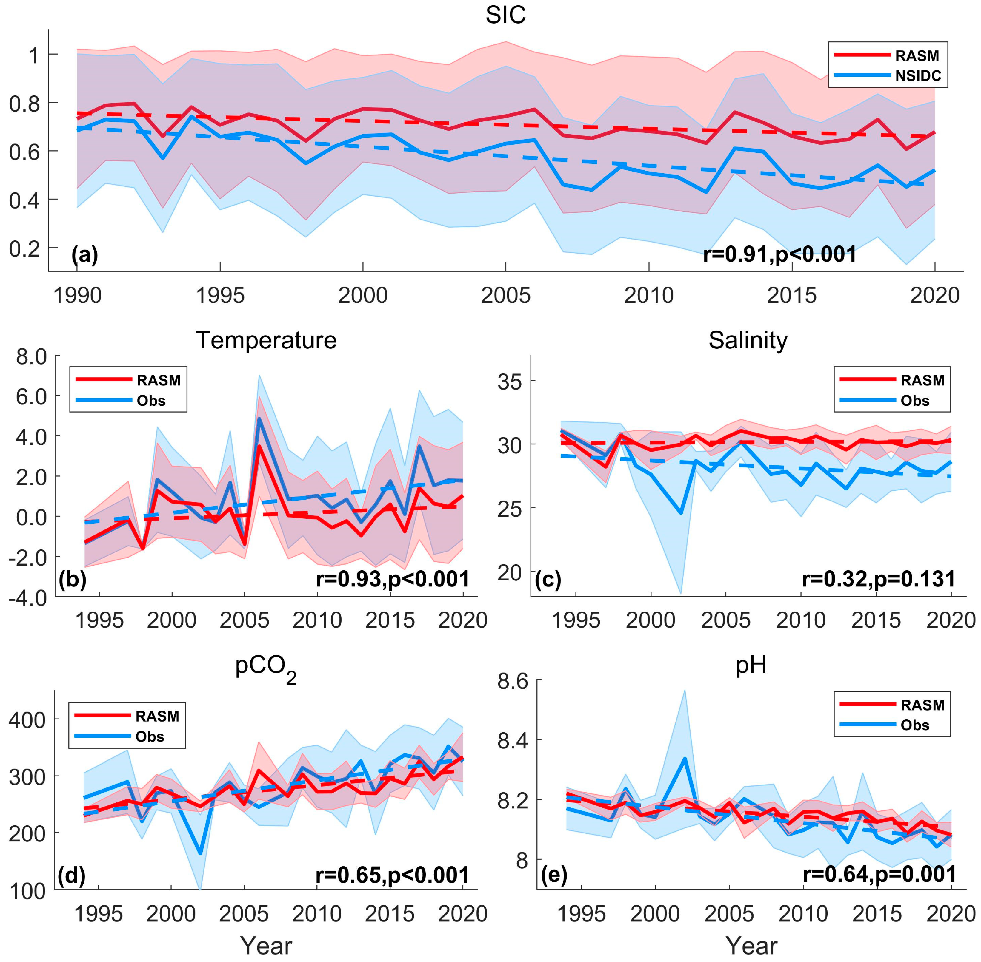
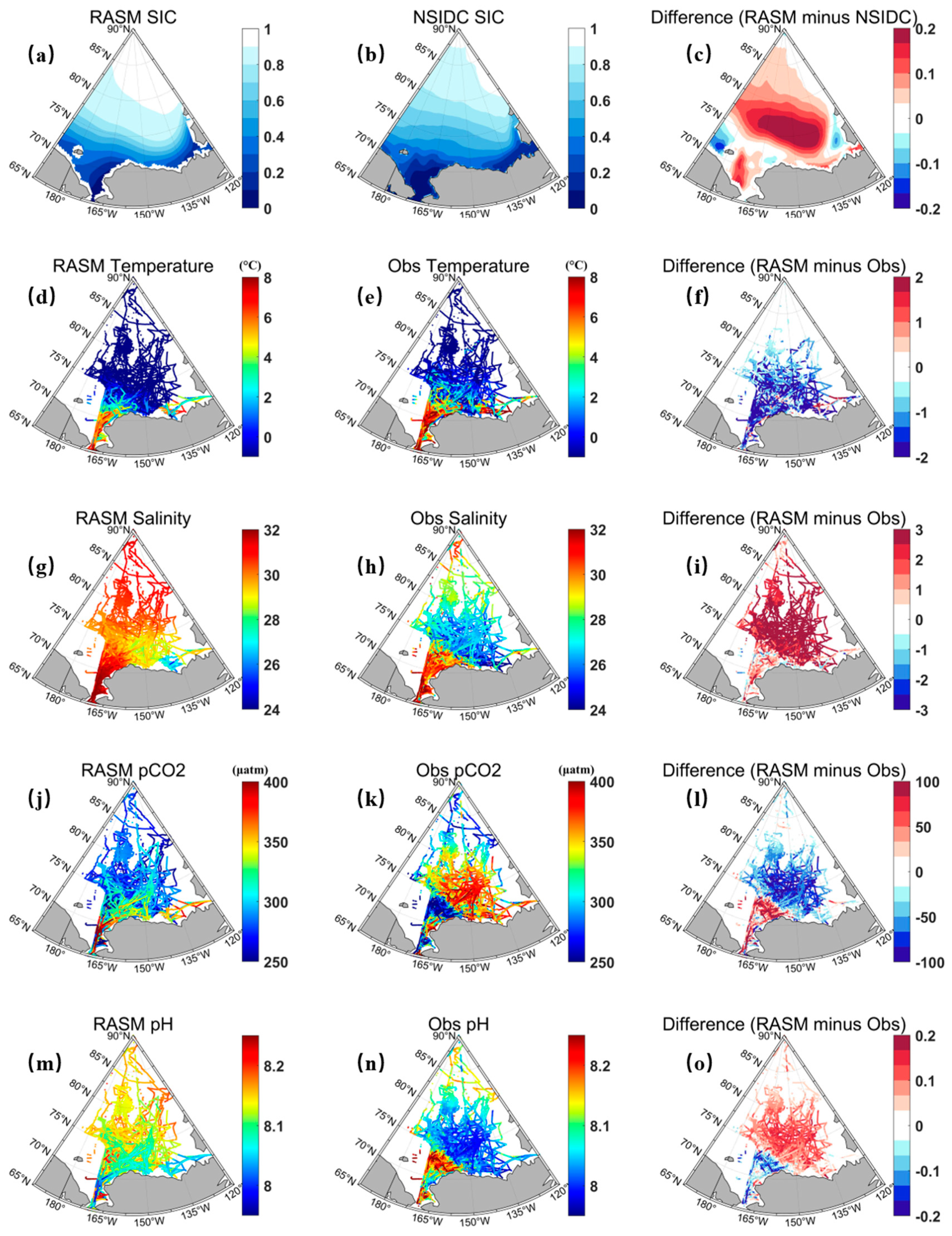
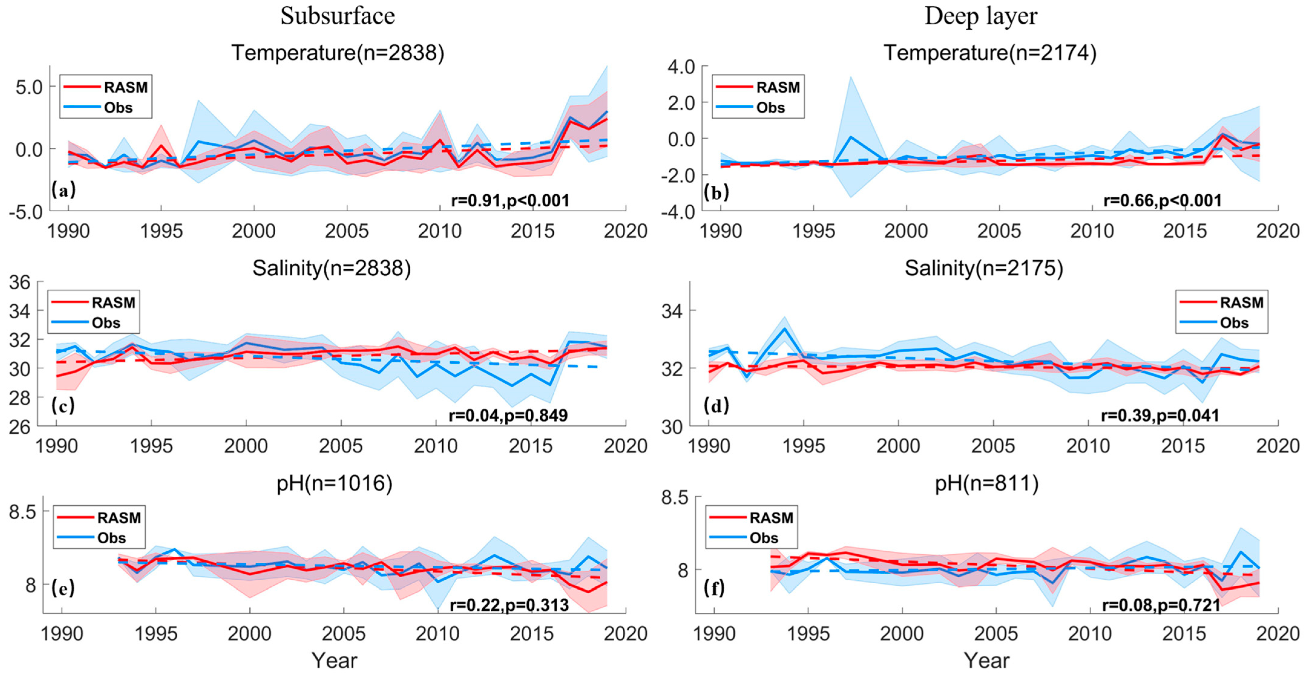
3.1. Model Validation

The RASM results are compared with observational data for the same period. The model showed a declining trend of SIC in the Western Arctic Ocean during summer (June–September average) from 1990 to 2020 (Figure 2a), comparable to the remote sensing SIC data with a significant correlation (r = 0.91, p < 0.001) and a root mean square error (RMSE) of 0.139. The model showed that the average SIC from 1990 to 2020 is the lowest in the southern Chukchi Sea, around 0.2, followed by the eastern coastal region of the BS (Figure 3a,b). The SIC distribution simulated by the RASM is similar to the data provided by remote sensing satellites (Figure 3a,b), but it is slightly higher than the remote sensing data in the CB region and areas to the north (Figure 3d). The modeled sea surface (0–20 m) temperature in the northwestern Arctic Ocean exhibited an increasing trend similar to the in situ observational data during July to October between 1994 and 2020 (Figure 2b), with a significant correlation between the two (r = 0.93, p < 0.001), and an RMSE of 0.92 °C. The modeled sea surface temperature is higher in the Chukchi Sea and the eastern BS, while temperatures in the CB and its northern regions are mostly around −1 °C, which closely matches the in situ observational data (Figure 3d,e). The modeled salinity matched the observed interannual variations before 2000 (Figure 2c), but showed some bias after that, especially a less download trend than the observations, likely because the model has bias to capture the increased convergence of the sea surface fresh water in the Beaufort Gyre. This causes RASM salinity to be higher in the CB than in the observed data (Figure 3i). The model showed a similar increasing trend of pCO₂ with in situ observational data (2.55 µatm/yr and 3.69 µatm/yr, respectively) in the Western Arctic Ocean (Figure 2d), comparable with a significant correlation (r = 0.65, p < 0.001) and an RMSE of 31.67 µatm. The modeled pCO₂ is higher along the coasts of the Chukchi Sea and BS compared to other regions, while it is slightly lower than the observational data in the CB (Figure 3l). The model showed a decreasing trend of surface pH similar to in situ observational data in the Western Arctic Ocean (Figure 2e), with rates of −0.0034/yr and −0.0054/yr, respectively, a significant correlation (r = 0.64, p = 0.001) and an RMSE of 0.053. The modeled surface pH distribution is similar to that of pCO₂, which is lower along the coasts of the Chukchi Sea and BS compared to other regions (Figure 3m). Overall, the RASM-simulated pH distribution can capture the spatial pattern of the observational data, with the exception of slightly higher values in the CB (Figure 3o). This discrepancy may be due to the model simulating a slightly higher SIC than observed (Figure 3c), preventing seawater from absorbing a large amount of AtmCO₂, thus causing an anomalous increase in pCO₂ and decrease in pH [28]. In the surface layer of the southern Canada Basin (70–75°N, 135–155°W, including the BS), the modeled pH decline rate of −0.0041/yr is comparable to a previous estimate of −0.0057/yr [11]. The model’s trends for SIC, SST, surface pCO₂, and surface pH correspond well with remote sensing and in situ observational data in most years (Figure 2b,d,e), indicating that the model effectively captures interannual variability comparable to observations.

The RASM-simulated subsurface (20–50 m) and deep layer (50–120 m) temperatures show the same increasing trend as the GLODAP water column data (Figure 4a,b), with correlation coefficients (r) of 0.91 and 0.66, and RMSE values of 0.069 and 0.078, respectively. The simulated subsurface and deep layer salinities match the GLODAP data well (Figure 4c,d) with RMSE values of 1.03 and 0.42, respectively. The simulated pH matches the long-term trend of the GLODAP data (Figure 4e,f), with RMSE values of 0.069 and 0.078, but the correlations between the model and data are not significant due to the limited and sparse data in the subsurface and deep layers, and complicated mechanisms involved.

To verify the distribution characteristics of upwelling, it is necessary to analyze the spatial distribution of EPV. Summer mean (June to September) EPV, 1990–2020, shows strong upwelling along the shelf break in the western BS, with a rate of approximately 6 cm/day, while most of the BS region, or the Beaufort Gyre subsidence area, shows downwelling at a rate of about −4 cm/day (Figure 5). The southward shift of the Beaufort Gyre subsidence area results in a negative regional average EPV, with downwelling dominance in certain years (Figure 6d). The modeled EPV is comparable to that calculated from daily sea level pressure reanalysis data and the NSIDC sea ice dataset by Ma et al. [30], which showed that most of the BS experienced downwelling in August at rates of −2 to −8 cm/day, except for the upwelling of 6–8 cm/day in the western BS along the shelf break. The modeled weak upwelling 78°N north of the Canadian Basin also agrees with the results from Ma et al. [30] and Zhong et al. [45]. The modeled distribution of upwelling and downwelling is generally similar to the ranges of previous studies [29,30,45,54,55]. Considering that the BS has a north–south continental slope, eastward-component winds are upwelling-favorable (Figure 4c,d), and EPV is significantly correlated with easterly wind frequency (EWF, r = 0.71, p < 0.05). This study uses EPV to characterize upwelling intensity and explore the relationship between pH and upwelling.

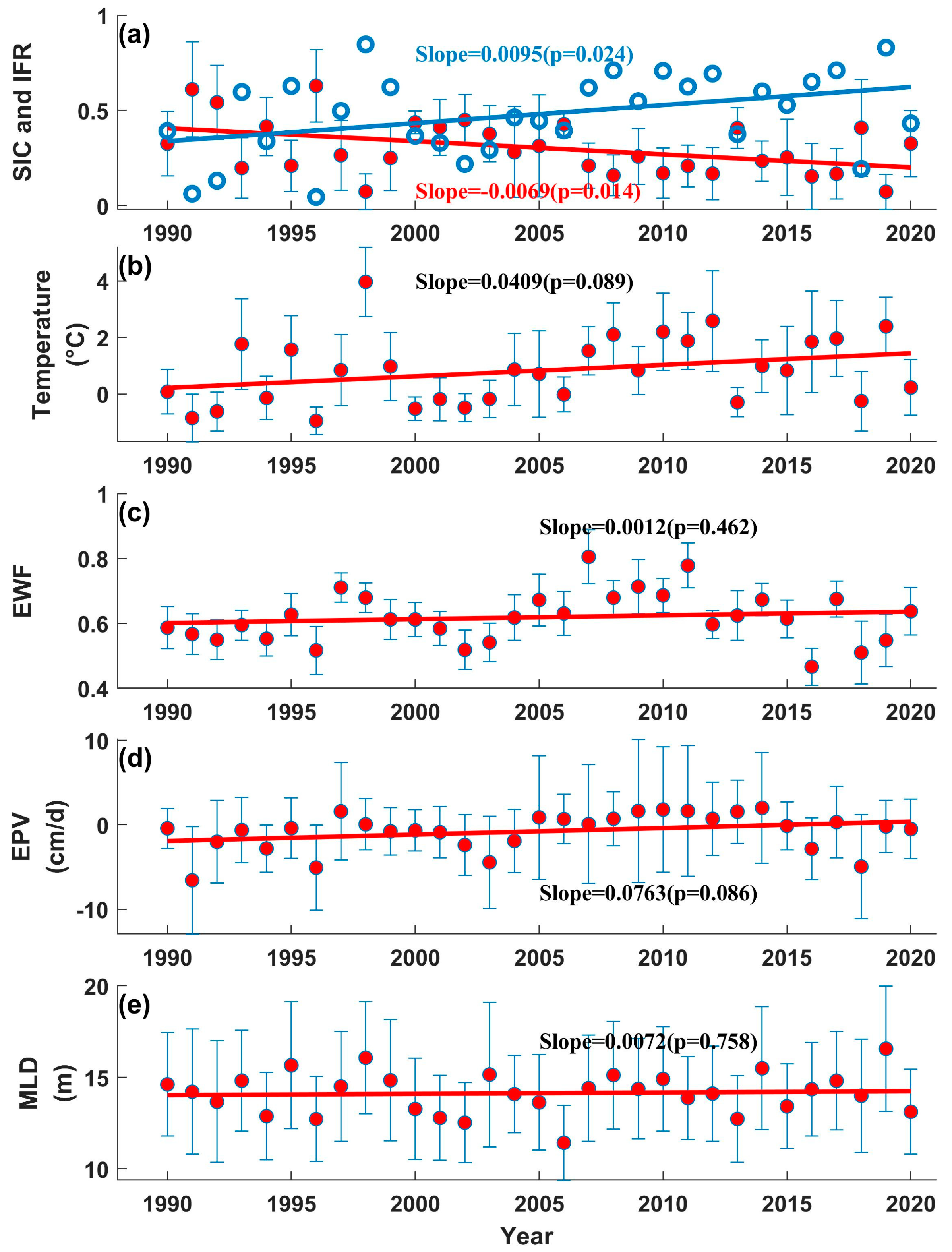
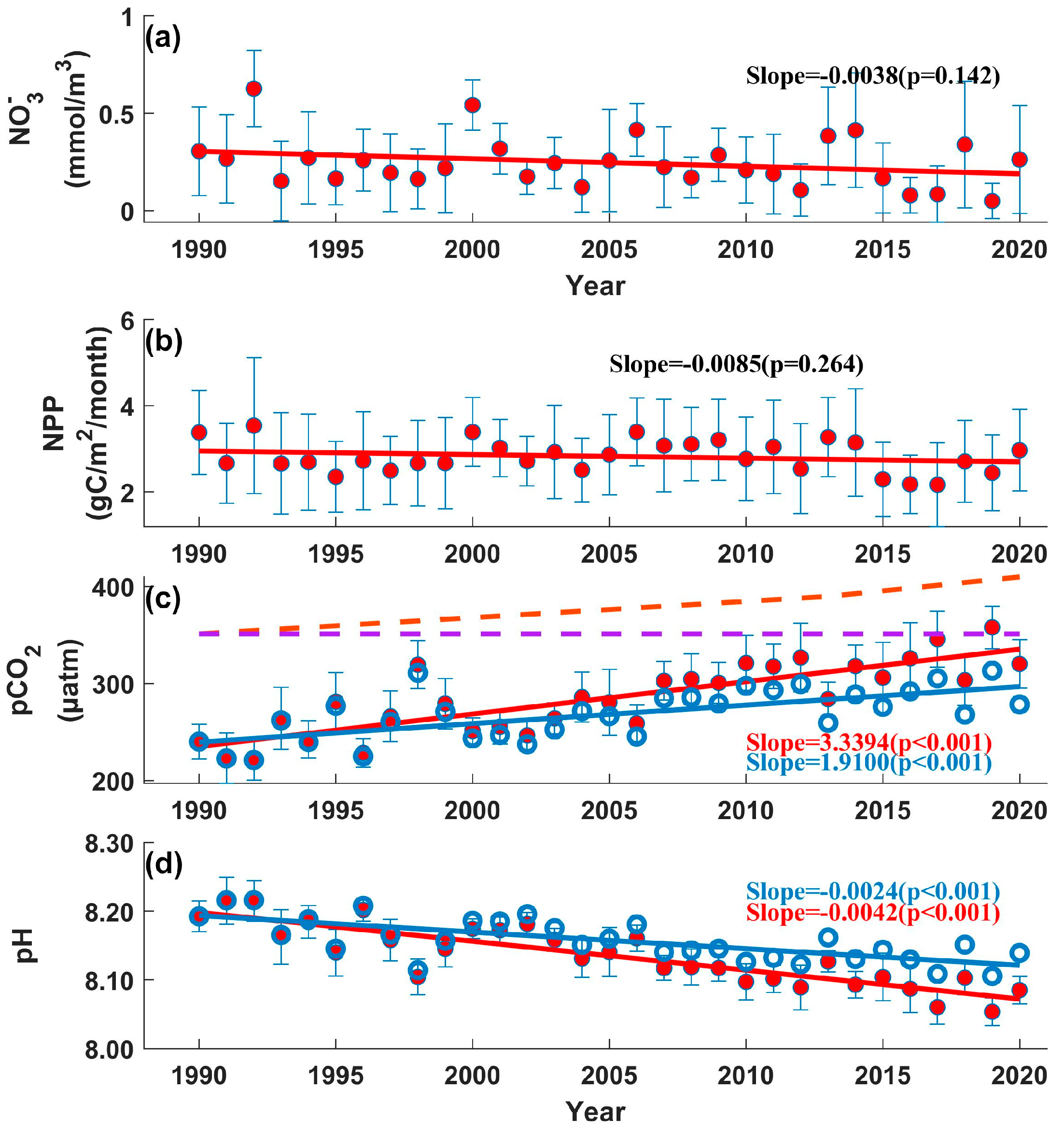
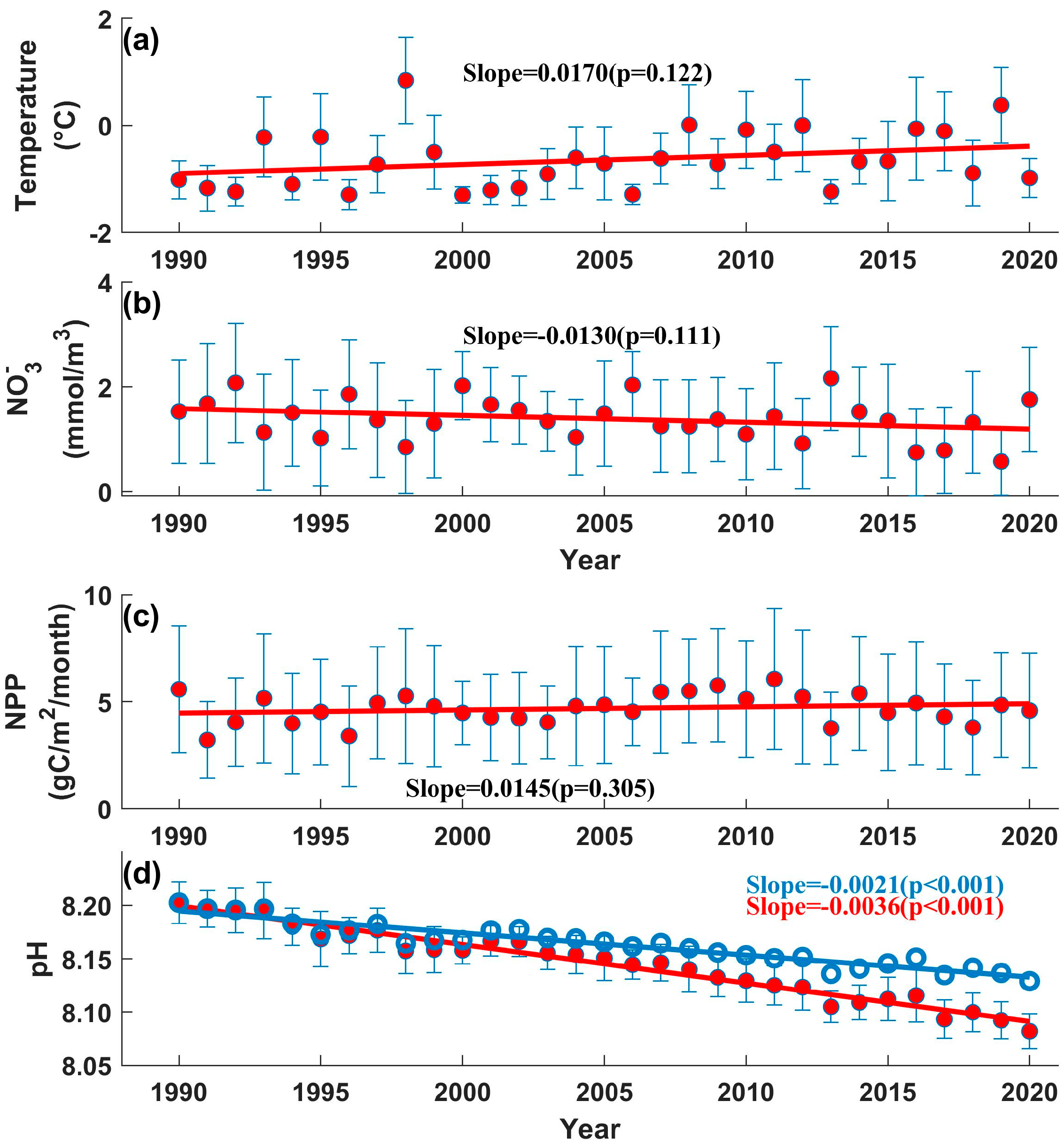
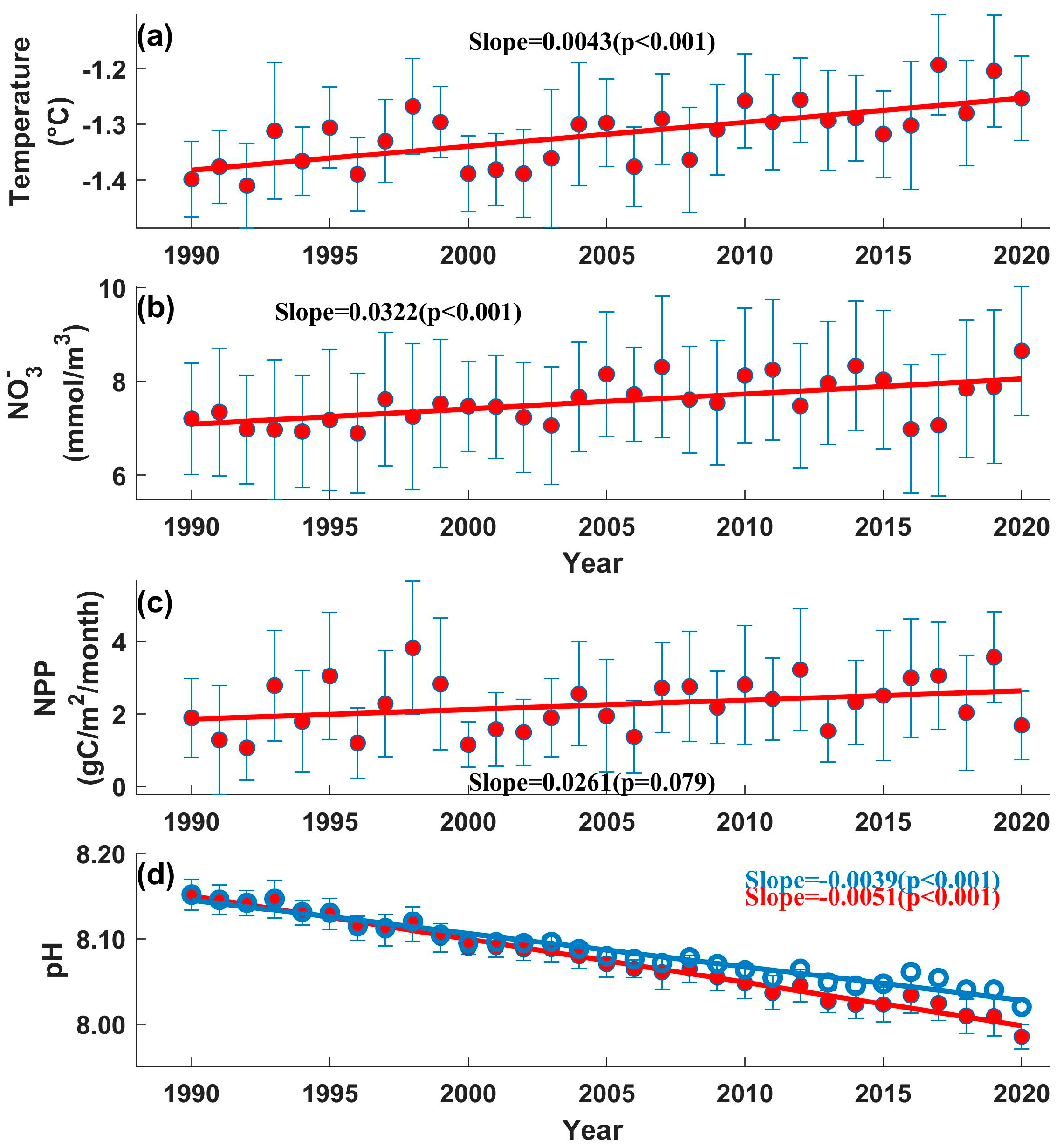
3.2. Long-Term Trends of Changes in the BS

The ecological environment in the BS has experienced rapid changes in recent years. Due to the high sensitivity of ocean acidification to the various forcing factors and feedback mechanisms among the atmosphere, sea ice, and ocean, it is necessary to analyze those factors and mechanisms in the BS. The RASM results indicate a significant decrease in SIC in the BS, with a rate of −0.0069/year, showing a reduction from an average of 0.4 in 1990 to 0.2 in 2020 (Figure 6a). In contrast, IFR increases significantly at a rate of 0.0095/year with a strong negative correlation with SIC changes (r = −0.97, p < 0.05). The surface layer temperature fluctuates considerably on an interannual basis, but its long-term trend remains insignificant (Figure 6b). EWF and EPV are significantly correlated (r = 0.72, p < 0.001), and neither exhibits a significant long-term trend (Figure 6c,d). MLD is significantly correlated with SIC (r = −0.73, p < 0.001), with an interannual range of 11–17 m but no significant long-term trend (Figure 6e). Nitrate concentrations in the surface layer are relatively lower than in the subsurface (20–50 m) and deep layers (50–120 m, Figure 7a, Figure 8b and Figure 9b), indicating that the surface seawaters are barren [31,56]. Consequently, surface NPP (averaging 2.82 gC/m²/month over 31 years) remains lower than in the subsurface layer (Figure 7b, Figure 8c and Figure 9c). As AtmCO₂ concentration rises and sea ice decreases, seawater absorbs AtmCO₂, resulting in a notable increasing trend in surface layer pCO₂ at a rate of 3.3394 µatm/year, similar to the rate derived from observational (3.58 ± 1.23 µatm/year) [28]. The long-term trend of surface pH in BS has a rate of change of −0.0042/year, with an average decrease from 8.20 in 1990 to 8.07 in 2020, showing an overall change of approximately 0.13 units. pH shows opposite variations to pCO₂ on interannual and decadal scales (Figure 7c,d).

The long-term trend in temperature is not significant in the subsurface layer (Figure 8a), but significant in the deep layer (Figure 9a). The NO₃ in the deep layer is the highest among the three layers and shows a significant upward trend (Figure 9b), while the NO₃ in the subsurface layer is second to that in the deep layer, with no significant long-term trend (Figure 8b). The subsurface layer has the highest NPP among the three layers, with a 31-year average of 4.69 gC/m²/month (Figure 8b). pH in the deep layer declines faster than in the subsurface (Figure 8d and Figure 9d), likely due to organic matter remineralization [57].

Acidification of BS seawater is due to changes in physical and biogeochemical variables. Multiple linear regressions are calculated after normalization of all variables in Equation (2). The regression results from case C show that the long-term trends of surface pH are affected by AtmCO₂, SIC, and MLD (

Table 1. Regression coefficients of the long-term trends of the seasonal mean (June to September) variables from 1990 to 2020 in Equation (2) after normalization at different layers in case C and S (bold values indicate p < 0.05). The percentage represents the relative contribution of the significant influencing factors.

Layer	AtmCO2 (Case C)	SIC (Case C)	EPV (Case C)	NPP (Case C)	MLD (Case C)	SIC (Case S)	EPV (Case S)	NPP (Case S)	MLD (Case S)
Surface	−0.668 −77.1%	0.346 20.7%	−0.087	0.084	−0.112 −2.2%	0.883 100%	−0.040	0.117	0.076
Subsurface	−0.956 −94.4%	−0.010	−0.176 −3.2%	0.154 2.4%	−0.067	0.990 69.6%	−0.291	0.654 30.4%	0.357
Deep layer	−1.006 −97.6%	−0.169	−0.158 −2.4%	−0.025	0.018	1.442	0.193	0.707	0.458

), with relative contributions (calculated as the square of its regression coefficient divided by the sum of the square of regression coefficients of all significant variables, and multiplied by 100%, and then adjusted by the sign of the regression coefficient) to the long-term pH trend of −77.1%, 20.7%, and −2.2% in case C, respectively. The negative sign in the relative contribution denotes the correlation is negative and the absolute value represents relative contribution. Given the relatively large contribution of AtmCO₂ concentration increases to the long-term trends of surface pH, a RASM case S (Figure 7c) was designed the same as control case C except the AtmCO₂ was kept at the 1990 level to identify the impact of increasing CO₂ on the carbonate system in the BS. Results from case S’s multiple linear regression show that the long-term trends of surface pH are only significantly affected by SIC (Table 1). These findings suggest that the drivers of the long-term reduction in summer surface pH are, primarily, the continuous increase in AtmCO₂ concentration, leading to sustained anthropogenic CO₂ absorption by seawater [27], and secondly, the reduction in sea ice, which enhances seawater uptake of AtmCO₂ [4,11,28]. These two drivers jointly contribute over 93% of the long-term decrease in sea surface pH.

Results from the multiple linear regression in case C (Table 1) show that the long-term trends of pH are significantly impacted by AtmCO₂, EPV, and NPP in the subsurface layer, with relative contributions of −94.4%, −3.2%, and 2.4%, respectively. The long-term trends of pH are significantly impacted by AtmCO₂ and EPV in the deep layer, with relative contributions of −97.4% and −2.4% (Table 1). These results indicate that the long-term decrease in summer pH from surface to deep layers is primarily driven by the increase in AtmCO₂ concentration.

Results from the multiple linear regression in case S (Table 1) show that the long-term trends of pH are significantly impacted by SIC and NPP in the subsurface layer (Table 1), with relative contributions of 69.6% and 30.4%, respectively. Without the influence of rising AtmCO₂, the long-term trend slope of surface pCO₂ decreases from 3.3394 to 1.9100 µatm/yr (Figure 7c). The long-term trends for surface, subsurface, and deep layer pH reduce from −0.0042, −0.0036, and −0.0051/yr to −0.0022, −0.0021, and −0.0039/yr (Figure 7d, Figure 8d and Figure 9d), representing rate reductions of 47.6%, 41.7%, and 23.5%, respectively. In case S, the sea surface pCO₂ is still increasing as it is lower than AtmCO₂, which allows seawater to continue absorbing anthropogenic CO₂. But by 2020, the air–sea CO₂ partial pressure difference of 54.2 µatm in case S is much lower than the 74.5 µatm in the case C (Figure 7c). Correspondingly, the long-term summer pH decline from 1990 to 2020 is slower in case S than in case C (Figure 7d).

3.3. Interannual Variation in Ph in the BS

In order to investigate pH interannual variations, multiple linear regressions of cases C and S are conducted after detrending and normalization of all variables in Equation (2). The regression results from both cases C and S show that pH interannual variability is significantly impacted by SIC and MLD in the surface layer (with relative contributions of 91.1% and −8.9% in case S), NPP and EPV in the subsurface layer (with relative contributions of 53.9% and −46.1% in case S) and EPV only in the deep layer (

Table 2. Similar to Table 1, but all variables are detrended first and then normalized. Bold values indicate p < 0.05. The percentage represents the relative contribution of the significant influencing factors.

Layer	SIC (Case C)	EPV (Case C)	NPP (Case C)	MLD (Case C)	SIC (Case S)	EPV (Case S)	NPP (Case S)	MLD (Case S)
Surface	0.606 78.0%	−0.113	0.180 6.9%	−0.266 −15.1%	0.662 91.1%	−0.130	0.155	−0.207 −8.9%
Subsurface	−0.005	−0.660 −35.7%	0.886 64.3%	−0.458	0.057	−0.756 −46.1%	0.818 53.9%	−0.298
Deep layer	−0.757	−0.623 −100%	0.215	−0.101	−0.677	−0.672 −100%	0.075	0.028

). The results suggest that although the long-term decrease in pH in case C is mainly attributed to the increasing AtmCO₂ and decreasing SIC, the pH interannual variations with decreasing amplitudes from surface to deep layers (Figure 7d, Figure 8d and Figure 9d) are modulated by different mechanisms other than AtmCO₂. Therefore, here we only use case S to study the interannual variation in pH. The statistically insignificant EPV influences on surface pH (Table 2) might be because upwelling-brought-up high NO₃ and DIC influence pH in opposite directions, and the strong vertical stratification caused by freshwater accumulation depressed the upwelling transport [31,56].

To investigate the effect of SIC on surface pH interannual variation in the BS, five highest (1996, 1991, 2018, 2013 and 1992) and five lowest SIC years (1998, 1993, 1995, 2019, and 2008) in case S were selected to compare. The differences (low SIC minus high SIC years) of the SIC, MLD and pH are −0.3775, 2.18 m and −0.0586. These differences in SIC, MLD, and pH are all statistically significant and reveal consistent mechanisms of changing pH with the multiple linear regression results (Table 2). The reduction in SIC increases the MLD and absorption of AtmCO₂ by seawater, which results in a statistically significant increase in pCO₂ and DIC (by 49.4 µatm and 51.4 mmol/m³) and decrease in pH.

Spatially, the SIC differences are the greatest in the eastern BS and southeastern CB, reaching up to −0.5 (Figure 10a). The differences in MLD are larger in the coastal areas of the eastern BS, approximately 3 m (Figure 10b). The highest pCO₂ and pH differences are similarly located in the eastern BS (Figure 10c,d). The differences in SIC, MLD, pCO₂, and pH are statistically significant in the eastern BS. However, the regions with largest differences in SIC and MLD are larger than those showing significant pH differences (Figure 10). The areas with notable pH differences are overlapping regions with the largest differences in both SIC and MLD, because both cause a statistically significant increase in pCO₂ and decrease in pH.

To explore why EPV drives statistically significant pH changes in the subsurface and deep layers (Table 2), five highest (1997, 2010, 2009, 2014 and 2011) and five lowest EPV years (2019, 1991, 1996, 2003 and 2016) were selected to compare. The EPV, SIC, subsurface NPP and DIC differences (high minus low EPV years) in the BS are statistically significant at 6.26 cm/day, −0.1851, 1.53 gC/m²/month and 18.5 mmol/m³ (

Table 3. Differences of NO₃, NPP, DIC and pH (high minus low EPV years) in different layers of BS in case S. Bold values indicate statistically significant differences with p < 0.05.

Difference	Subsurface Layer	Deep Layer
NO3 (mmol/m3)	0.01	0.64
NPP (gC/m2/month)	1.53	0.43
DIC (mmol/m3)	18.5	11.2
pH	−0.0035	−0.0094

), respectively. The subsurface NPP differences are statistically significant in most regions of BS and the eastern CB (Figure 11b) with magnitudes up to 3.00 gC/m²/month. Subsurface NPP consumes the upwelling-brought-up NO₃ from deep layers and results in no significant subsurface NO₃ differences in BS (Figure 11a,b). DIC shows the largest differences along the continental slope between 125 and 145°W (Figure 11c) because the upwelling-brought-up higher DIC outweighs the NPP consumption on DIC. The regional mean subsurface pH difference in BS is not statistically significant (Table 3), similar to the multiple linear regression results (Table 2), except for 135°W and 145°W of BS with statistically significant pH differences (Figure 11d). This is because higher EPV influences subsurface pH through two opposing mechanisms: (1) the biological mechanism, where upwelling elevates NO₃-rich waters, causing a significant increase in NPP [31], which raises pH; (2) physical mechanism, where upwelling lifts DIC-rich waters, leading to a decrease in pH. The pH differences are negative (Table 3), indicating that the second mechanism is stronger than the first, although the differences are not statistically significant.

In the deep layer, NO₃ and DIC differences are statistically significant in BS with a magnitude of 0.64 mmol/m³ and 11.2 mmol/m³, respectively (Table 3). Due to the reduced light intensity at depth layer [58], NPP shows a much lower increase than in the subsurface layer (Table 3). The pH differences are negative but statistically insignificant, similar to the subsurface layer. Other factors, such as the intrusion of Pacific Winter Water between approximately 100 and 250 m [59], might also influence the statistical significances here. Spatially, the deep layer region with statistically significant pH differences along the slopes at 140° and 125°W (Figure 11a,c,d) resembles that of NO₃, NPP and DIC, indicating that only upwelling-driven physical mechanisms dominate in this limited slope region.

The zonally averaged cross-section differences (high minus low EPV years) of NO₃ in BS are the largest and statistically significant in the deep layer near the shelf break (Figure 12a). The subsurface NO₃ differences near the shelf (<72°N) are 0.01 mmol/m³, smaller than the 0.64 mmol/m³ in the deep layer (Figure 12a). The smaller subsurface NO₃ differences are due to significant biological consumption, resulting in a corresponding subsurface NPP differences of 1.53 gC/m²/month (Table 3), much larger than those in the other layers. As Ekman-transported high NO₃ diminishes with increasing distance northward away from shelf break, the NO₃ differences in the CB center decrease exponentially to nearly zero (Figure 12a). The NPP differences align with the NO₃ differences, showing a northward decrease in both the surface and subsurface layers.

The DIC difference is the largest and statistically significant along the slope at depths of 20–120 m (Figure 12c), while the pH difference is maximal and statistically significant at 60–120 m, similar to NO₃ (Figure 12a,d). Influenced by increased subsurface NPP, pH exhibits positive differences, transported northward to the CB center by Ekman (Figure 12d). High EPV corresponds to strong upwelling near the shelf break, lifting NO₃-rich and DIC-rich water from depths greater than 120 m, resulting in negative pH differences in the deep layers (Figure 12a,c,d). The differences in NO₃ and DIC show a pathway of nutrient-rich and DIC-rich waters movement up along the shelf break, and then a northward Ekman transport pathway in the surface and subsurface layers and subsidence in the north basin region [31] (Figure 12a,b). In the 50–120 m slope region, NO₃ and DIC differences are causally linked to pH differences, consistent with the multiple linear regression results, indicating that upwelling-driven physical processes dominate in these areas. The pH difference is statistically significant only along a narrow slope at 60–120 m (Figure 12d), leading to the statistically insignificant pH differences averaged in the deep layer (Table 3). In the subsurface near the shelf break, the NPP differences and NO₃ differences are clearly the dominant drivers of the positive pH differences (Figure 12). The regionally averaged subsurface pH differences are not statistically significant in Table 3 because the biological effects are not dominant in other BS regions away from the shelf break, consistent with the linear regression results (Table 2).

4. Discussion

The acidification rate in the Northwest Arctic Ocean is excessively fast, and in 2015, acidification exceeded the threshold (aragonite saturation less than 1) [11], leading to the dissolution of calcifying organisms’ shells and fish bones [24]. It is urgent to examine the long-term trends and interannual changes in acidification rates. The long-term acidification of the Northwest Arctic Ocean is mainly driven by increasing AtmCO₂ concentrations and the rapid decline in sea ice [6,11], while enhanced NPP may mitigate the rate of acidification [17]. Furthermore, variations in MLD due to seasonal sea ice melt could influence acidification [34]. The BS, a marginal sea of the Northwest Arctic Ocean with a north–south slope, experiences prevailing easterly winds that drive upwelling (EPV > 0). However, the effects of MLD and EPV on BS acidification, as well as the relative contributions of various factors to long-term trends and interannual variations in acidification, require further research.

In this paper, the RASM results are validated by satellite remote sensing data and in situ observations for the summer (June–September) of 1990–2020. Multiple linear regressions of the RASM case C and case S were used to clarify the effects and relative contributions of different factors including AtmCO₂, SIC, EPV, NPP and MLD on the long-term trends and interannual variations in pH in different layers of the BS. The multiple linear regression results for case C show that AtmCO₂ significantly influences the long-term trend of pH from the surface to the deep layers, with relative contributions of −77.1%, −94.4%, and −97.4% (here, a negative sign denotes negative correlation), respectively. This indicates that the continuous increase in AtmCO₂ dominates the long-term decline in pH from the surface to the deep layers in the BS. SIC has a significant impact on the long-term trend on in the surface pH, with a relative contribution of 20.7%. Although MLD has a significant negative impact on the long-term trend of surface pH, NPP has a significant positive impact on the long-term trend of subsurface pH, and EPV has a significant negative impact on the long-term trend of subsurface and deep layer pH, their relative contributions are all less than 5%, indicating relatively minor influences on the long-term pH trend.

For the interannual variation in pH from the surface to the deep layers, AtmCO₂ is not a significant factor according to the multiple regression results for case C and case S because AtmCO₂ shows little interannual variations, although it shows a long-term trend and seasonal cycle. In the surface layer, the factors that significantly influence the interannual variation in pH are SIC and MLD, with relative contributions of 91.1% and −8.9%, respectively. This suggests that SIC has a significant positive effect on surface pH, and its reduction leads to increased CO₂ absorption by surface seawater, thereby lowering seawater pH. In the subsurface, NPP and EPV contribute 53.9% and −46.1%, respectively, to the interannual variation in pH, with opposing effects. In the deep layer, only EPV has a significant impact on the interannual variation in pH.

We compared the differences (low SIC years minus high SIC years) in the distribution of SIC, MLD, surface pCO₂ and surface pH between the five high SIC years and the five low SIC years to analyze the significant effect of low SIC on pH. We also compared the differences (high EPV years minus low EPV years) in the spatial distribution of NO₃, NPP, DIC and pH between the five high and five low EPV years to analyze the effect of the two opposing processes induced by high EPV on pH at the shelf break.

The persistently increasing AtmCO₂ and declining sea ice cover have driven the long-term pH decline in BS in the past three decades. Sea ice reduction also significantly affects the interannual variability of surface pH, while upwelling is a significant driver in subsurface and deep layers pH variations in the BS. Global warming accelerates permafrost thawing and coastal erosion, increasing riverine inputs of organic carbon [60,61]. The Mackenzie River’s input of carbon and nutrients into the BS may significantly influence the long-term trends and interannual variability of surface and subsurface pH. The intrusion of Pacific Winter Water, approximately at a 100–250 m depth [59], may also be a significant factor influencing pH in the BS. Therefore, it is essential to gain a more extensive understanding of the acidification in the BS in order to address future risks and challenges.

5. Conclusions

This study used the RASM, validated by remote sensing data and in situ observations, to investigate the long-term trends and interannual variations in pH in the BS and its significant influencing factors, with the following conclusions:

Multiple linear regression results from the RASM case C show that the main factors significantly influencing the long-term surface pH decline are AtmCO₂ and SIC, with relative contributions of −77.1% and 20.7%, respectively. In the subsurface and deep layers, the main factor is still AtmCO₂, with relative contributions over −94.4%. Since the rising AtmCO₂ concentration is the dominant driver for the long-term decline in summer pH from surface to deep layers in the BS, we designed the RASM case S, similar to the control case C, except AtmCO₂ is kept at the 1990 level. The regression results from case S show that the long-term trends of pH are significantly affected by SIC only in the surface and by SIC and NPP in the subsurface, with relative contributions of 69.6% and 30.4% (no significant factor in the deep layer). The above results suggest that even if the AtmCO₂ concentration remained at 1990 levels, the summer pH would still exhibit a long-term decline trend from 1990 to 2020, with rates of −0.0022, −0.0021, and −0.0039/yr for the surface, subsurface, and deep layers, respectively, primarily driven by SIC reduction, although these declining rates of pH are slower than those in case C (−0.0042, −0.0036, and −0.0051/yr for the surface, subsurface, and deep layers, respectively). And the Arctic Ocean has not yet reached equilibrium with the accumulated AtmCO₂ partial pressure from 1990 due to the ongoing climate warming.

In contrast to the nearly linearly increasing AtmCO₂ over the last three decades, the ocean pH shows more interannual variations in addition to the long-term trends. The multiple linear regression results from both cases C and S indicate that the interannual variations in pH are significantly affected by SIC and MLD in the surface (with relative contributions of 91.1% and −8.9% in case S), NPP and EPV in the subsurface (with relative contributions of 53.9% and −46.1% in case S) and EPV only in the deep layer.

To investigate the effect of SIC on surface pH interannual variation in the BS, five highest and five lowest SIC years in case S were selected to compare. The differences (low minus high SIC years) of the SIC, MLD and pH are statistically significant, revealing consistent mechanisms of changing pH with the multiple linear regression results. The reduction in SIC in BS increases the MLD and absorption of AtmCO₂ by seawater, which results in a statistically significant increase in pCO₂, and decrease in pH. Spatially, the areas with notable pH differences are overlapping regions with the largest differences in both SIC and MLD, located in the eastern BS, because both cause a statistically significant increase in pCO₂ and decrease in pH.

To investigate the effect of EPV on subsurface and deep layer pH interannual variations in the BS, five highest and five lowest EPV years in case S were selected to compare. The EPV, subsurface NPP and DIC differences (high minus low EPV years) in the BS are statistically significant. The regional mean subsurface pH difference in BS is statistically insignificant, similar to the multiple linear regression results, except for 135°W and 145°W of BS with statistically significant pH differences. This is because higher EPV influences subsurface pH through two opposing mechanisms: (1) biological mechanism, where upwelling elevates NO₃-rich waters, causing a significant increase in NPP, which raises pH; (2) physical mechanism, where upwelling lifts DIC-rich waters, leading to a decrease in pH. The subsurface pH differences are negative, indicating that the second mechanism is stronger than the first, although the resulting pH differences are not statistically significant. Influenced by increased subsurface NPP, the zonally averaged cross-section differences in pH exhibit positive differences near the shelf break, indicating that the biological effects are dominant due to the upwelling effect. In the deep slope region, NO₃ and DIC differences are causally linked to pH differences, consistent with the multiple linear regression results, indicating that upwelling-driven physical processes dominate in these areas. The pH difference is statistically significant only along the narrow shelf break at 60–120 m, but the regionally averaged pH differences are statistically insignificant.

References

1. Budget, G.C. Global Carbon Budget 2023; Global Carbon Budget: Exeter, UK, 2023. [Google Scholar]
2. Sabine, C.L.; Feely, R.A.; Gruber, N.; Key, R.M.; Lee, K.; Bullister, J.L.; Wanninkhof, R.; Wong, C.S.; Wallace, D.W.R.; Tilbrook, B.; et al. The Oceanic Sink for Anthropogenic CO2. Science 2004, 305, 367–371. [Google Scholar] [CrossRef] [PubMed]
3. Takahashi, T.; Sutherland, S.C.; Wanninkhof, R.; Sweeney, C.; Feely, R.A.; Chipman, D.W.; Hales, B.; Friederich, G.; Chavez, F.; Sabine, C.; et al. Climatological Mean and Decadal Change in Surface Ocean pCO2, and Net Sea–Air CO2 Flux over the Global Oceans. Deep Sea Res. Part II 2009, 56, 554–577. [Google Scholar] [CrossRef]
4. Cai, W.-J.; Chen, L.; Chen, B.; Gao, Z.; Lee, S.H.; Chen, J.; Pierrot, D.; Sullivan, K.; Wang, Y.; Hu, X.; et al. Decrease in the CO2 Uptake Capacity in an Ice-Free Arctic Ocean Basin. Science 2010, 329, 556–559. [Google Scholar] [CrossRef] [PubMed]
5. Orr, J.C.; Fabry, V.J.; Aumont, O.; Bopp, L.; Doney, S.C.; Feely, R.A.; Gnanadesikan, A.; Gruber, N.; Ishida, A.; Joos, F. Anthropogenic Ocean Acidification over the Twenty-First Century and Its Impact on Calcifying Organisms. Nature 2005, 437, 681–686. [Google Scholar] [CrossRef]
6. Yamamoto−Kawai, M.; McLaughlin, F.A.; Carmack, E.C.; Nishino, S.; Shimada, K. Aragonite Undersaturation in the Arctic Ocean: Effects of Ocean Acidification and Sea Ice Melt. Science 2009, 326, 1098–1100. [Google Scholar] [CrossRef]
7. Feely, R.A.; Sabine, C.L.; Lee, K.; Berelson, W.; Kleypas, J.; Fabry, V.J.; Millero, F.J. Impact of Anthropogenic CO2 on the CaCO3 System in the Oceans. Science 2004, 305, 362–366. [Google Scholar] [CrossRef]
8. Walsh, J.E. Climate of the Arctic Marine Environment. Ecol. Appl. 2008, 18, S3–S22. [Google Scholar] [CrossRef]
9. Yasunaka, S.; Siswanto, E.; Olsen, A.; Hoppema, M.; Watanabe, E.; Fransson, A.; Chierici, M.; Murata, A.; Lauvset, S.K.; Wanninkhof, R. Arctic Ocean CO2 Uptake: An Improved Multiyear Estimate of the Air–Sea CO2 Flux Incorporating Chlorophyll a Concentrations. Biogeosciences 2018, 15, 1643–1661. [Google Scholar] [CrossRef]
10. Takahashi, T.; Sutherland, S.C.; Chipman, D.W.; Goddard, J.G.; Ho, C.; Newberger, T.; Sweeney, C.; Munro, D.R. Climatological Distributions of pH, pCO2, Total CO2, Alkalinity, and CaCO3 Saturation in the Global Surface Ocean, and Temporal Changes at Selected Locations. Mar. Chem. 2014, 164, 95–125. [Google Scholar] [CrossRef]
11. Qi, D.; Ouyang, Z.; Chen, L.; Wu, Y.; Lei, R.; Chen, B.; Feely, R.A.; Anderson, L.G.; Zhong, W.; Lin, H.; et al. Climate Change Drives Rapid Decadal Acidification in the Arctic Ocean from 1994 to 2020. Science 2022, 377, 1544–1550. [Google Scholar] [CrossRef]
12. Duffey, A.; Mallett, R.; Irvine, P.J.; Tsamados, M.; Stroeve, J. ESD Ideas: Arctic Amplification’s Contribution to Breaches of the Paris Agreement. Earth Syst. Dyn. 2023, 14, 1165–1169. [Google Scholar] [CrossRef]
13. Peng, G.; Matthews, J.L.; Yu, J.T. Sensitivity Analysis of Arctic Sea Ice Extent Trends and Statistical Projections Using Satellite Data. Remote Sens. 2018, 10, 230. [Google Scholar] [CrossRef]
14. Else, B.G.T.; Papakyriakou, T.N.; Galley, R.J.; Mucci, A.; Gosselin, M.; Miller, L.A.; Shadwick, E.H.; Thomas, H. Annual Cycles of p CO2sw in the Southeastern Beaufort Sea: New Understandings of Air-sea CO2 Exchange in Arctic Polynya Regions. J. Geophys. Res. 2012, 117, C00G13. [Google Scholar] [CrossRef]
15. Wang, H.; Lin, P.; Pickart, R.S.; Cross, J.N. Summer Surface CO2 Dynamics on the Bering Sea and Eastern Chukchi Sea Shelves From 1989 to 2019. JGR Ocean. 2022, 127, e2021JC017424. [Google Scholar] [CrossRef]
16. Lewis, K.M.; Van Dijken, G.L.; Arrigo, K.R. Changes in Phytoplankton Concentration Now Drive Increased Arctic Ocean Primary Production. Science 2020, 369, 198–202. [Google Scholar] [CrossRef]
17. Tu, Z.; Le, C.; Bai, Y.; Jiang, Z.; Wu, Y.; Ouyang, Z.; Cai, W.; Qi, D. Increase in CO2 Uptake Capacity in the Arctic Chukchi Sea During Summer Revealed by Satellite-Based Estimation. Geophys. Res. Lett. 2021, 48, e2021GL093844. [Google Scholar] [CrossRef]
18. Hufford, G.L. On Apparent Upwelling in the Southern Beaufort Sea. J. Geophys. Res. 1974, 79, 1305–1306. [Google Scholar] [CrossRef]
19. Else, B.G.T.; Galley, R.J.; Papakyriakou, T.N.; Miller, L.A.; Mucci, A.; Barber, D. Sea Surface p CO2 Cycles and CO2 Fluxes at Landfast Sea Ice Edges in Amundsen Gulf, Canada. J. Geophys. Res. 2012, 117, C007901. [Google Scholar] [CrossRef]
20. Tremblay, J.-É.; Bélanger, S.; Barber, D.G.; Asplin, M.; Martin, J.; Darnis, G.; Fortier, L.; Gratton, Y.; Link, H.; Archambault, P.; et al. Climate Forcing Multiplies Biological Productivity in the Coastal Arctic Ocean: Upwelling and productivity in the arctic. Geophys. Res. Lett. 2011, 38, L18604. [Google Scholar] [CrossRef]
21. Fabry, V.J.; McClintock, J.B.; Mathis, J.T.; Grebmeier, J.M. Ocean Acidification at High Latitudes: The Bellwether. Oceanography 2009, 22, 160–171. [Google Scholar] [CrossRef]
22. Kroeker, K.J.; Kordas, R.L.; Crim, R.N.; Singh, G.G. Meta-analysis Reveals Negative yet Variable Effects of Ocean Acidification on Marine Organisms. Ecol. Lett. 2010, 13, 1419–1434. [Google Scholar] [CrossRef] [PubMed]
23. Harvey, B.P.; Gwynn−Jones, D.; Moore, P.J. Meta-analysis Reveals Complex Marine Biological Responses to the Interactive Effects of Ocean Acidification and Warming. Ecol. Evol. 2013, 3, 1016–1030. [Google Scholar] [CrossRef] [PubMed]
24. Kroeker, K.J.; Kordas, R.L.; Crim, R.; Hendriks, I.E.; Ramajo, L.; Singh, G.S.; Duarte, C.M.; Gattuso, J. Impacts of Ocean Acidification on Marine Organisms: Quantifying Sensitivities and Interaction with Warming. Glob. Change Biol. 2013, 19, 1884–1896. [Google Scholar] [CrossRef]
25. Bates, N.R.; Astor, Y.M.; Church, M.J.; Currie, K.; Dore, J.E.; González−Dávila, M.; Lorenzoni, L.; Muller−Karger, F.; Olafsson, J.; Santana−Casiano, J.M. A Time-Series View of Changing Surface Ocean Chemistry Due to Ocean Uptake of Anthropogenic CO2 and Ocean Acidification. Oceanography 2014, 27, 126–141. [Google Scholar] [CrossRef]
26. Yamamoto, A.; Kawamiya, M.; Ishida, A.; Yamanaka, Y.; Watanabe, S. Impact of Rapid Sea-Ice Reduction in the Arctic Ocean on the Rate of Ocean Acidification. Biogeosciences 2012, 9, 2365–2375. [Google Scholar] [CrossRef]
27. Terhaar, J.; Torres, O.; Bourgeois, T.; Kwiatkowski, L. Arctic Ocean Acidification over the 21st Century Co-Driven by Anthropogenic Carbon Increases and Freshening in the CMIP6 Model Ensemble. Biogeosciences 2021, 18, 2221–2240. [Google Scholar] [CrossRef]
28. Ouyang, Z.; Qi, D.; Chen, L.; Takahashi, T.; Zhong, W.; DeGrandpre, M.D.; Chen, B.; Gao, Z.; Nishino, S.; Murata, A.; et al. Sea-Ice Loss Amplifies Summertime Decadal CO2 Increase in the Western Arctic Ocean. Nat. Clim. Change 2020, 10, 678–684. [Google Scholar] [CrossRef]
29. Meneghello, G.; Marshall, J.; Timmermans, M.-L.; Scott, J. Observations of Seasonal Upwelling and Downwelling in the Beaufort Sea Mediated by Sea Ice. J. Phys. Oceanogr. 2018, 48, 795–805. [Google Scholar] [CrossRef]
30. Ma, B.; Steele, M.; Lee, C.M. Ekman Circulation in the A Rctic O Cean: Beyond the B Eaufort G Yre. JGR Ocean. 2017, 122, 3358–3374. [Google Scholar] [CrossRef]
31. Xu, A.; Jin, M.; Wu, Y.; Qi, D. Response of Nutrients and Primary Production to High Wind and Upwelling-Favorable Wind in the Arctic Ocean: A Modeling Perspective. Front. Mar. Sci. 2023, 10, 1065006. [Google Scholar] [CrossRef]
32. Mathis, J.T.; Pickart, R.S.; Byrne, R.H.; McNeil, C.L.; Moore, G.W.K.; Juranek, L.W.; Liu, X.; Ma, J.; Easley, R.A.; Elliot, M.M.; et al. Storm-induced Upwelling of High p CO2 Waters onto the Continental Shelf of the Western Arctic Ocean and Implications for Carbonate Mineral Saturation States. Geophys. Res. Lett. 2012, 39, L07606. [Google Scholar] [CrossRef]
33. Mol, J.; Thomas, H.; Myers, P.G.; Hu, X.; Mucci, A. Inorganic Carbon Fluxes on the Mackenzie Shelf of the Beaufort Sea. Biogeosciences 2018, 15, 1011–1027. [Google Scholar] [CrossRef]
34. Peralta−Ferriz, C.; Woodgate, R.A. Seasonal and Interannual Variability of Pan-Arctic Surface Mixed Layer Properties from 1979 to 2012 from Hydrographic Data, and the Dominance of Stratification for Multiyear Mixed Layer Depth Shoaling. Prog. Oceanogr. 2015, 134, 19–53. [Google Scholar] [CrossRef]
35. Jin, M.; Deal, C.; Maslowski, W.; Matrai, P.; Roberts, A.; Osinski, R.; Lee, Y.J.; Frants, M.; Elliott, S.; Jeffery, N.; et al. Effects of Model Resolution and Ocean Mixing on Forced Ice-Ocean Physical and Biogeochemical Simulations Using Global and Regional System Models. JGR Ocean. 2018, 123, 358–377. [Google Scholar] [CrossRef]
36. Jin, M.; Popova, E.E.; Zhang, J.; Ji, R.; Pendleton, D.; Varpe, Ø.; Yool, A.; Lee, Y.J. Ecosystem Model Intercomparison of Under-ice and Total Primary Production in the A Rctic O Cean. JGR Ocean. 2016, 121, 934–948. [Google Scholar] [CrossRef]
37. Steele, M.; Morley, R.; Ermold, W. PHC: A Global Ocean Hydrography with a High-Quality Arctic Ocean. J. Clim. 2001, 14, 2079–2087. [Google Scholar] [CrossRef]
38. Harada, Y.; Kamahori, H.; Kobayashi, C.; Endo, H.; Kobayashi, S.; Ota, Y.; Onoda, H.; Onogi, K.; Miyaoka, K.; Takahashi, K. The JRA-55 Reanalysis: Representation of Atmospheric Circulation and Climate Variability. J. Meteorol. Soc. Japan. Ser. II 2016, 94, 269–302. [Google Scholar] [CrossRef]
39. Moore, J.K.; Doney, S.C.; Lindsay, K. Upper Ocean Ecosystem Dynamics and Iron Cycling in a Global Three-dimensional Model. Glob. Biogeochem. Cycles 2004, 18, GB4028. [Google Scholar] [CrossRef]
40. DiGirolamo, N.; Parkinson, C.L.; Cavalieri, D.J.; Gloersen, P.; Zwally, H.J. Sea Ice Concentrations from Nimbus-7 SMMR and DMSP SSM/I-SSMIS Passive Microwave Data, Version 2; NASA National Snow and Ice Data Center Distributed Active Archive Center: Boulder, CO, USA, 2022. [Google Scholar]
41. Olsen, A.; Key, R.M.; Van Heuven, S.; Lauvset, S.K.; Velo, A.; Lin, X.; Schirnick, C.; Kozyr, A.; Tanhua, T.; Hoppema, M. The Global Ocean Data Analysis Project Version 2 (GLODAPv2)—An Internally Consistent Data Product for the World Ocean. Earth Syst. Sci. Data 2016, 8, 297–323. [Google Scholar] [CrossRef]
42. Key, R.M.; Olsen, A.; van Heuven, S.; Lauvset, S.K.; Velo, A.; Lin, X.; Schirnick, C.; Kozyr, A.; Tanhua, T.; Hoppema, M. Global Ocean Data Analysis Project, Version 2 (GLODAPv2). Ornl/Cdiac-162 Ndp-093. 2015. Available online: https://glodap.info/index.php/data-access/ (accessed on 3 June 2024).
43. Kobayashi, C.; Iwasaki, T. Brewer-Dobson Circulation Diagnosed from JRA-55. JGR Atmos. 2016, 121, 1493–1510. [Google Scholar] [CrossRef]
44. Yang, J. The Seasonal Variability of the Arctic Ocean Ekman Transport and Its Role in the Mixed Layer Heat and Salt Fluxes. J. Clim. 2006, 19, 5366–5387. [Google Scholar] [CrossRef]
45. Zhong, W.; Steele, M.; Zhang, J.; Zhao, J. Greater Role of Geostrophic Currents in Ekman Dynamics in the Western Arctic Ocean as a Mechanism for Beaufort Gyre Stabilization. JGR Ocean. 2018, 123, 149–165. [Google Scholar] [CrossRef]
46. McPhee, M.G. An Analysis of Pack Ice Drift in Summer. In Sea Ice Processes Models; Pritchard, R., Ed.; University of Washington Press: Seattle, WA, USA, 1980; pp. 62–75. [Google Scholar]
47. Lee, K.; Wanninkhof, R.; Feely, R.A.; Millero, F.J.; Peng, T. Global Relationships of Total Inorganic Carbon with Temperature and Nitrate in Surface Seawater. Glob. Biogeochem. Cycles 2000, 14, 979–994. [Google Scholar] [CrossRef]
48. Bozec, Y.; Thomas, H.; Schiettecatte, L.-S.; Borges, A.V.; Elkalay, K.; De Baar, H.J.W. Assessment of the Processes Controlling the Seasonal Variations of Dissolved Inorganic Carbon in the North Sea. Limnol. Oceanogr. 2006, 51, 2746–2762. [Google Scholar] [CrossRef]
49. Lee, K.; Tong, L.T.; Millero, F.J.; Sabine, C.L.; Dickson, A.G.; Goyet, C.; Park, G.; Wanninkhof, R.; Feely, R.A.; Key, R.M. Global Relationships of Total Alkalinity with Salinity and Temperature in Surface Waters of the World’s Oceans. Geophys. Res. Lett. 2006, 33, L19605. [Google Scholar] [CrossRef]
50. Carter, B.R.; Feely, R.A.; Williams, N.L.; Dickson, A.G.; Fong, M.B.; Takeshita, Y. Updated Methods for Global Locally Interpolated Estimation of Alkalinity, pH, and Nitrate. Limnol. Ocean. Methods 2018, 16, 119–131. [Google Scholar] [CrossRef]
51. Li, B.; Watanabe, Y.W.; Yamaguchi, A. Spatiotemporal Distribution of Seawater pH in the North Pacific Subpolar Region by Using the Parameterization Technique. JGR Ocean. 2016, 121, 3435–3449. [Google Scholar] [CrossRef]
52. Williams, N.L.; Juranek, L.W.; Johnson, K.S.; Feely, R.A.; Riser, S.C.; Talley, L.D.; Russell, J.L.; Sarmiento, J.L.; Wanninkhof, R. Empirical Algorithms to Estimate Water Column pH in the Southern Ocean. Geophys. Res. Lett. 2016, 43, 3415–3422. [Google Scholar] [CrossRef]
53. Hauri, C.; Irving, B.; Dupont, S.; Pagés, R.; Hauser, D.D.; Danielson, S.L. Insights into Carbonate Environmental Conditions in the Chukchi Sea. Biogeosciences 2024, 21, 1135–1159. [Google Scholar] [CrossRef]
54. Dewey, S.; Morison, J.; Kwok, R.; Dickinson, S.; Morison, D.; Andersen, R. Arctic Ice-Ocean Coupling and Gyre Equilibration Observed with Remote Sensing. Geophys. Res. Lett. 2018, 45, 1499–1508. [Google Scholar] [CrossRef]
55. Zhang, J.; Steele, M.; Runciman, K.; Dewey, S.; Morison, J.; Lee, C.; Rainville, L.; Cole, S.; Krishfield, R.; Timmermans, M.-L.; et al. The Beaufort Gyre Intensification and Stabilization: A Model-Observation Synthesis: Beaufort gyre stabilization. J. Geophys. Res. Ocean. 2016, 121, 7933–7952. [Google Scholar] [CrossRef]
56. Timmermans, M.-L.; Toole, J.M. The Arctic Ocean’s Beaufort Gyre. Annu. Rev. Mar. Sci. 2023, 15, 223–248. [Google Scholar] [CrossRef] [PubMed]
57. Qi, D.; Chen, B.; Chen, L.; Lin, H.; Gao, Z.; Sun, H.; Zhang, Y.; Sun, X.; Cai, W. Coastal Acidification Induced by Biogeochemical Processes Driven by Sea-Ice Melt in the Western Arctic Ocean. Polar Sci. 2020, 23, 100504. [Google Scholar] [CrossRef]
58. Laney, S.R.; Krishfield, R.A.; Toole, J.M. The Euphotic Zone under Arctic Ocean Sea Ice: Vertical Extents and Seasonal Trends. Limnol. Oceanogr. 2017, 62, 1910–1934. [Google Scholar] [CrossRef]
59. Zhong, W.; Steele, M.; Zhang, J.; Cole, S.T. Circulation of Pacific Winter Water in the Western Arctic Ocean. JGR Ocean. 2019, 124, 863–881. [Google Scholar] [CrossRef]
60. Guo, L.; Macdonald, R.W. Source and Transport of Terrigenous Organic Matter in the Upper Yukon River: Evidence from Isotope (d13C, D14C, and d15N) Composition of Dissolved, Colloidal, and Particulate Phases. Glob. Biogeochem. Cycles 2006, 20, 1–12. [Google Scholar] [CrossRef]
61. Cai, W.-J.; Hu, X.; Huang, W.-J.; Murrell, M.C.; Lehrter, J.C.; Lohrenz, S.E.; Chou, W.-C.; Zhai, W.; Hollibaugh, J.T.; Wang, Y. Acidification of Subsurface Coastal Waters Enhanced by Eutrophication. Nat. Geosci. 2011, 4, 766–770. [Google Scholar] [CrossRef]
Figure 1. Distribution of in situ observational data stations (pink dots) in the Western Arctic Ocean. The study area is Beaufort Sea (BS, red box), with Canadian Basin (CB, purple box) to the north. Black solid lines are isobaths 100 m, 500 m and 3000 m.
Remotesensing 17 00866 g001
Figure 2. Interannual variability of sea surface variables, (a) SIC, (b) temperature (°C), (c) salinity, (d) pCO2 (µatm) and (e) pH in the Western Arctic Ocean (range shown in Figure 1, 65−90°N, 175°E−120°W) for the RASM (red) and observational data (blue). (a) Observational sea ice concentration data are from NSIDC product; (be) observational data are in situ observations. Correlation coefficients and p-values between the model outputs and observations are located in the lower right corner. The dashed lines indicate the long-term trends of the variables.
Remotesensing 17 00866 g002
Figure 3. Comparison of RASM and observed data over 1990−2020 for sea surface variables. The first column shows the model output for (a) SIC, (d) temperature, (g) salinity, (j) pCO2, and (m) pH; the second column corresponds to the observational data for (b) SIC, (e) temperature, (h) salinity, (k) pCO2, and (n) pH, and the third column represents the difference between the model and the observational data for (c) SIC, (f) temperature, (i) salinity, (l) pCO2, and (o) pH.
Remotesensing 17 00866 g003
Figure 4. Comparison of subsurface and deep layer variables from RASM (red) and GLODAP observation dataset (blue): (a) subsurface temperature, (b) deep layer temperature, (c) subsurface salinity, (d) deep layer salinity, (e) subsurface pH; (f) deep layer pH. Correlation coefficients and p-values between the model outputs and observations are located in the lower right corner. The dashed lines indicate the long-term trends of the variables. Shading indicates the standard deviation of the variables. n denotes the number of observation data.
Remotesensing 17 00866 g004
Figure 5. Ekman vertical pumping velocity (EPV, cm/day) averaged over June–September 1990–2020. Arrows indicate the Ekman transport velocity (m/s) within the Ekman layer. The boxed areas in the figure are consistent with the boxed areas in Figure 1.
Remotesensing 17 00866 g005
Figure 6. The interdecadal trends in summer averages (June–September) of variables in the BS surface layer (0–20 m) in the case C: (a) SIC (red circles and solid line) and IFR (blue circles and solid line), (b) temperature (°C), (c) EWF, (d) EPV (cm/day), and (e) MLD (m). Positive values of EPV denote upwelling and negative values denote downwelling. Red dots indicate the mean value at each time point, and the blue bar error line indicates the standard deviation for its season. The solid red line is the rate of change in the linear fit.
Remotesensing 17 00866 g006
Figure 7. The interdecadal trends in summer averages (June–September) of variables in the BS surface layer (0–20 m): (a) surface NO3 (mmol/m3), (b) NPP (gC/m2/month), (c) pCO2 (µatm), and (d) pH. All data are from case C, except for the purple dashed line in (c) and the blue circles and lines in (c,d), which represent data from case S. In (c), the orange and purple dashed lines represent AtmCO2 concentration in case C and S, respectively. Red dots indicate the mean value at each time point, and the blue bar error line indicates the standard deviation for its season. The solid red line is the rate of change in the linear fit.
Remotesensing 17 00866 g007
Figure 8. The interdecadal trends in summer averages (June–September) of various variables in the BS subsurface layer (20–50 m): (a) temperature (°C), (b) NO3 (mmol/m3), (c) NPP (gC/m2/month), and (d) pH. All data are from the RASM case C, except for the blue circles and lines in (d), which represent data from case S. Red dots indicate the mean value at each time point, and the blue bar error line indicates the standard deviation for its season. The solid red line is the rate of change in the linear fit.
Remotesensing 17 00866 g008
Figure 9. Similar to Figure 8, but applies to the deep layer (50–120 m): (a) temperature (°C), (b) NO3 (mmol/m3), (c) NPP (gC/m2/month), and (d) pH. All data are from the RASM case C, except for the blue circles and lines in (d), which represent data from case S. Red dots indicate the mean value at each time point, and the blue bar error line indicates the standard deviation for its season. The solid red line is the rate of change in the linear fit.
Remotesensing 17 00866 g009
Figure 10. Differences (low minus high) between high (1996, 1991, 2018, 2013 and 1992) and low (1998, 1993, 1995, 2019, and 2008) SIC years in the surface layers of the BS and CB regions in case S: (a) SIC, (b) MLD (m), (c) pCO2 (µatm), and (d) pH. Black dots indicate statistical significance (p < 0.05). Red boxes indicate BS region, gray boxes indicate CB region.
Remotesensing 17 00866 g010
Figure 11. Differences (high minus low EPV years) of (a) NO3 (mmol/m3), (b) NPP (gC/m2/month), (c) DIC (mmol/m3), and (d) pH in case S. from top to bottom representing surface, subsurface, and deep layers. Black dots indicate statistically significant differences (p < 0.05). Red boxes indicate BS region, gray boxes indicate CB region.
Remotesensing 17 00866 g011
Figure 12. Latitudinally averaged differences (high minus low EPV years) of (a) NO3 (mmol/m3), (b) NPP (gC/m3/month), (c) DIC (mmol/m3), and (d) pH of case S. The gray dashed lines denote 20 m and 50 m depths. Black dots indicate statistically significant differences (p < 0.05).
Remotesensing 17 00866 g012