Technical Note

An Adaptive Constant Acceleration Model for Maneuvering Target Tracking

1
Air and Missile Defense College, Air Force Engineering University, Xi’an 710051, China
2
High Speed Aerodynamic Institute, China Aerodynamics Research and Development Center, Mianyang 621000, China
*
Author to whom correspondence should be addressed.
Remote Sens. 2025, 17(5), 850; https://doi.org/10.3390/rs17050850
Submission received: 3 December 2024 / Revised: 20 February 2025 / Accepted: 26 February 2025 / Published: 28 February 2025
(This article belongs to the Special Issue Array and Signal Processing for Radar)

Abstract

:
An adaptive constant acceleration (ACA) model is proposed for the maneuvering target tracking problem. Based on the Taylor series expansion of acceleration, we establish the relationship between the Jerk and the velocity as well as the acceleration so that the maneuvering acceleration variance is approximated by the components in the state error covariance matrix. Then, the latter one is connected with the process noise, and the adaptive adjustment of the ACA model is realized. Combining with the strong tracking square-root cubature filter (ST-SCKF) in our previous work, an ACA-ST-SCKF is developed. The simulation results show that the proposed filter possesses better adaptability, tracking accuracy and lower computational complexity compared with the adaptive current statistical (ACS) model-based ST-SCKF, the modified CS (MCS) model-based ST-SCKF, and the IMM-based STF-SCKF.

1. Introduction

The maneuvering target tracking is of critical importance for many aspects. However, such a problem is always an intractable task [1]. The studies have shown that the means of tracking accuracy improvement can be roughly divided into two parts. One is to improve the adaptivity of the motion model, and another is to improve the precision of the filter. Aiming at the first issue, the singer model [2], the current statistical (CS) model [3], and the Jerk model [4] are successively proposed. The CS model has a better ability to characterize the maneuvering feature than the others [1]. However, the CS model has some limitations, i.e., need of prior parameters and lack of adaptivity [5,6]. As such, many modified CS models are put forward. Refs. [7,8,9] utilize the membership function to adaptively correct the maximum acceleration in the CS model. Ref. [10] adopts the residual error to adjust the maneuvering frequency. Ref. [11] exploits the state estimate deviation to represent the acceleration disturbance quantity. However, one parameter (the maximum acceleration or the maneuvering frequency) is just concentrated in [7,8,9,10,11], and the other is neglected. More importantly, these methods [7,8,9,10,11] are peripheral and do not touch the innate character of the CS model. Though ref. [5,6] introduced the Jerk input estimate to essentially modify the CS model, the augment of the state vector naturally leads to additional computational burden.
On the other hand, in the nonlinear system, a series of the Gaussian approximation filters [12,13,14] are developed, e.g., the unscented Kalman filter (UKF) [12], the Gauss–Hermite quadrature filter (GHQF) [13], and the cubature Kalman filter (CKF) [14]. Compared with the extended Kalman filter (EKF) [15], the avoidance of Jacobian matrix and higher precision are two prominent features in these filters [12,13,14]. To further improve the robustness when faced with abrupt change, the strong tracking filter (STF) [16] is widely exploited. Recently, ref. [5] fully re-deduced the introduced position of the fading factor and demonstrated its effectiveness. Ref. [17] considers a linear pairwise Markov model (PMM) with Student’s t noise to model non-cooperative single target tracking without clutter and missed detections and develops a filter for the case where noise statistics are accurately known. In Ref. [18], a new Gaussian approximate filter is proposed to address a nonlinear system with colored non-stationary heavy-tailed measurement noise. A novel robust Student’s t-based Kalman filter is proposed to track maneuvering target in Ref. [19]. In Ref. [20], a new robust Kalman filtering framework for a linear system with non-Gaussian heavy-tailed and/or skewed state and measurement noises is proposed through modeling one-step prediction and likelihood probability density functions as Gaussian scale mixture (GSM) distributions. Moreover, a new variational adaptive Kalman filter with a Gaussian–inverse–Wishart mixture distribution is proposed for a class of linear systems with both partially unknown state and measurement noise covariance matrices in Ref. [21]. Ref. [22] derives a novel robust EC distributions-based Kalman filtering framework. In Ref. [23], a sliding window variational outlier-robust Kalman filter based on Student’s t-noise modeling is presented to distinguish model uncertainties from measurement outliers as they only exploit the current measurement.
Aiming at the issues in the motion model, an adaptive constant acceleration (ACA) model is proposed in this paper. According to the Taylor series expansion, we establish the approximation relationship between the Jerk component and the velocity as well as the acceleration. Then, the state error covariance matrix is fully exploited to online correct the process noise covariance, so that the adaptive adjustment of the proposed model is realized. Furthermore, to improve the filter stability, the ST-SCKF over ACA model is built based on our early work [5,6]. A large number of simulations verify the superior performance of the proposed filter.

2. CS Modeling

The CS model and the measurement model in the nonlinear system are separately given by [3,5,6]
x k + 1 = F k x k + U k a ¯ k + w k
and
z k = h x k + v k
The descriptions of parameters in (1) and (2) are shown in Table 1. The CS model utilizes a modified Rayleigh distribution to describe the statistical properties of maneuver acceleration, which allows for adaptive adjustment of the process noise based on the acceleration valuation at the previous moment. When the target maneuvers with a certain acceleration, the range of the acceleration changes in the next moment is limited and can only be within the domain of the current acceleration. The CS model can better inverse the change of target maneuver characteristics based on the current statistical characteristics of the target maneuver. For more details, readers can refer to [3,7,8,9,10,11].
The variance of maneuvering acceleration complies with the modified Rayleigh distribution as follows:
σ a 2 = 4 π π a max a ¯ k + 1 2 ,   a ¯ k + 1 0 4 π π a max + a ¯ k + 1 2 ,   a ¯ k + 1 < 0
However, in the CS model, a ¯ k + 1 is inaccessible. Therefore, the following approximation is suggested [1]:
a ¯ k + 1 a ^ k + 1 = E a k + 1 Z k E a k Z k = a ^ k
where E is the expectation operator, Z k is the set of measurements from time 0 to time k , and a ^ k is the acceleration estimate at the kth interval. Equation (4) implies that, in the CS model, a ¯ k + 1 is defined as the acceleration prediction on the condition of Z k , and a ^ k is used to approximate a ^ k + 1 and a ¯ k + 1 . Thus, (3) is expressed as follows:
σ a 2 = 4 π π a max a ^ k 2 ,   a ^ k 0 4 π π a max + a ^ k 2 ,   a ^ k < 0
By observing (5) and Q k in Table 1, we know that two prior parameters, i.e., the maximum acceleration a ± max and the maneuvering frequency α, play important roles in the CS model. If they are preset a little larger, the performance will be highly degraded when faced with the stable state, whereas the small values cannot track the strong maneuver preciously. As such, the CS model needs to be modified in application.

3. ACA Model

When faced with the near CA motion, the CA model with constant-mean Gaussian process noise is appropriate. By contrast, the colored process noise is more fit for the acceleration with the ascertain maneuver and stochastic maneuver. However, in the colored noise models, e.g., the Singer model and the CS model, prior parameters are necessary. According to [24], we know that the CA model can replace the colored noise model on the condition of appropriate process noise. Therefore, an ACA model is put forward to approximate the CS model, and the state error covariance matrix is fully used for the realization of adaptive adjustment.
On the basis of Taylor series expansion, the acceleration item is given by the following expression:
a t = a t 0 + 1 1 ! a 1 t 0 t t 0 + 1 2 ! a 2 t 0 t t 0 2 + + 1 n ! a n t 0 t t 0 n
where a 1 t 0 is the Jerk value in time t 0 . a n t 0 is the nth order derivative of a t . If we let t 0 = k T and t = k + 1 T , where T is the sample interval, (6) is expressed as follows [6]:
a k + 1 = a k + T a k 1 + T 2 2 ! a k 2 + + T n n ! a k n
Therefore, (4) can be rewritten as follows:
a ¯ k + 1 E a k + 1 Z k = E a k Z k + E a k 1 Z k + E a k 2 Z k T 2 2 ! + + E a k n Z k T n n ! = a ^ k + T a ^ k 1 + T 2 2 ! a ^ k 2 + + T n n ! a ^ k n
Meanwhile, (3) is rewritten as follows:
σ a , k 2 = 4 π π a ˜ k + T a ˜ k 1 + T 2 2 ! a ˜ k 2 + + T n n ! a ˜ k n 2
where a ˜ k n is the estimate error of a k n .
The discrete-time state expression of CA model is expressed as follows:
x k + 1 = F CA x k + w k CA
where w k CA ~ N ( 0 , Q k CA ) .
Q k CA = C q σ k 2 I 2 q CA
where C q is the designed parameter. q CA is the process noise covariance matrix with the noise intensity of 1.
q CA = T 5 / 20 T 4 / 8 T 3 / 6 T 4 / 8 T 3 / 3 T 2 / 2 T 3 / 6 T 2 / 2 T
When the error components higher than the Jerk order are elided, σ k 2 in (9) can be approximated by the following expression.
σ k 2 = 4 π π a ˜ k a ˜ k T + T 2 a ˜ k 1 a ˜ k 1 T + T a ˜ k a ˜ k 1 T + T a ˜ k 1 a ˜ k T
where a ˜ k 1 is the estimate error of the Jerk component. Due to the dimensional limitation of the CA model, Jerk error variance is inaccessible. Here, a k = a k 1 in the CA model is utilized, and a t is approximated by (14) when t = k T and t 0 = k 1 T .
a t x ˙ t x ˙ t 0 t t 0
The derivative of (14) is as follows:
a 1 t x ¨ t t t 0 x ˙ t x ˙ t 0 t t 0 2
where a 1 t is able to be expressed as the linear function of y.
a 1 t 1 t t 0 2 1 t t 0 1 t t 0 2 y
where y = [ x ˙ t , x ¨ t , x ˙ t 0 ] T . The discrete form of (16) is as follows:
a 1 t 1 T 2 1 T 1 T 2 y k
where y k = [ x ˙ k , x ¨ k , x ˙ k 1 ] T . Therefore, we have the following relationship between a ˜ k 1 and y ˜ k :
σ k 2 = 4 π π x ¨ ˜ k x ¨ ˜ k T + b y ˜ k x ¨ ˜ k T T + x ¨ ˜ k y ˜ k T b T T + b y ˜ k y ˜ k T b T T 2
On the assumption of E y ˜ k y ˜ k 1 T = 0 , the components in (18) are able to be represented by the components in the estimate error covariance matrix.
x ¨ ˜ k x ¨ ˜ k T f 1 E x ¨ ˜ k x ¨ ˜ k T = P k x ¨ , x ¨
y ˜ k x ¨ ˜ k T f 2 E x ˜ k x ¨ ˜ k T = P k x ¨ , x ˙ , P k x ¨ , x ¨ , 0 T
x ¨ ˜ k y ˜ k T f 2 E x ¨ ˜ k x ˜ k T = P k x ¨ , x ˙ , P k x ¨ , x ¨ , 0
and
y ˜ k y ˜ k T f 3 E x ˜ k x ˜ k T = P k x ˙ , x ˙ P k x ¨ , x ˙ 0 P k x ¨ , x ˙ P k x ¨ , x ¨ 0 0 0 P k 1 x ˙ , x ˙
According to (19)–(22), σ k 2 is expressed as follows:
σ k 2 = 4 π π f 1 E x ¨ ˜ k x ¨ ˜ k T + b f 2 E x ˜ k x ¨ ˜ k T T + f 2 E x ¨ ˜ k x ˜ k T b T T + b f 3 E x ˜ k x ˜ k T b T T 2
where b = 1 T 2 1 T 1 T 2 . However, shorter T means weaker maneuver for observers. Thus, the parameter C q is designed as C q = T 2 to make the process noise directly proportional to the sample interval T .
Equation (23) shows that the Jerk variance and the cross-covariance between Jerk and acceleration are approximated by the velocity variance, acceleration variance, and their cross-covariance. Thereby, the state error covariance is fully utilized for the adaptive adjustment, and tracking performance, when faced with different maneuver states, is able to be guaranteed.

4. Tracking Precision Analysis

Just for simplicity, the proposed ACA model is analyzed within a linear system and continuous time region. The nonlinear system can be handled accordingly. The state model and measurement model are separately denoted as follows:
x ˙ t = F CA x t + 0 , 0 , 1 T w t
and
z t = H x t + 1 , 0 , 0 T v t
where x ( t ) = [ x ( t ) , x ˙ ( t ) , x ¨ ( t ) ] T , and
F CA = 0 1 0 0 0 1 0 0 0
where H = 1 , 0 , 0 , w t N 0 , Q , and v t N 0 , R . In the Kalman filter, the recursive state estimate is calculated as follows:
x ˙ ^ t = F CA x ^ t + K CA t z t H x ^ t = F CA K CA t H x ^ t + K CA t z t
where K CA t is the Kalman gain matrix.
When the Kalman filter arrives at the steady state, K CA t tends to a constant matrix K CA . If the initial state is 0 and the Laplace transform of state is x s , then the Laplace transform of Kalman filtering error is expressed as follows:
x ˜ s = x s x ^ s = I s I F CA + K CA H 1 K CA H x s + s I F CA + K CA H 1 K CA ς v t x ˜ d s + x ˜ r s
where
x ˜ d s = 1 s 3 + k 1 s 2 + k 2 s + k 3 s 3 x s s 2 s + k 1 x ˙ s s s 2 + k 1 s + k 2 x ¨ s
where x ˜ d s and x ˜ r s are the steady model error and the steady measurement error, respectively. k 1 , k 2 , and k 3 are elements in the Kalman gain matrix K CA . Combing (1), (24), (28), and (29), we know that the dynamic errors of ACA model and CS model are equivalent, and the main difference is the gain matrix. Then, we discuss the steady model error in the following three conditions:
(1) When the input is the unit pulse acceleration, we have x ¨ ( s ) = 1 , x ˙ ( s ) = 1 / s , and x ( s ) = 1 / s 2 , and thus
x ˜ d t | t = lim s s s 3 s 3 + k 1 s 2 + k 2 s + k 3 1 s 2 = 0
Similarly, we have x ˙ ˜ d ( t ) | t = 0 , and x ¨ ˜ d ( t ) | t = 0 .
(2) When the input is the unit step acceleration, we have x ¨ ( s ) = 1 / s , x ˙ ( s ) = 1 / s 2 , and x ˙ ( s ) = 1 / s 3 , and thus
x ˜ d t | t = lim s s s 3 s 3 + k 1 s 2 + k 2 s + k 3 1 s 3 = 0
Similarly, we have x ˙ ˜ d ( t ) | t = 0 , and x ¨ ˜ d ( t ) | t = 0 .
(3) When the input is the unit slope acceleration, we have x ¨ ( s ) = 1 / ( 2 s 2 ) , x ˙ ( s ) = 1 / ( 2 s 3 ) , and x ˙ ( s ) = 1 / ( 2 s 4 ) , and thus
x ˜ d t | t = lim s s s 3 s 3 + k 1 s 2 + k 2 s + k 3 1 2 s 4 = 1 2 k 3
Similarly, we have x ˙ ˜ d ( t ) | t = k 1 2 k 3 , and x ¨ ˜ d ( t ) | t = k 2 2 k 3 .
From the three conditions, we know that the steady model error of the ACA model and the CS model tend to zero when the input is the unit pulse or the unit step acceleration, whereas the steady model error of two models are constant in the unit slope acceleration input. However, in the simulations, we will see the superior performance of the proposed ACA model.

5. Simulations and Results

The simulations are run on a single Inter (R) Core (TM) i7-4790 CPU (3.6 GHz) processor with 8 GB memory, MATLAB 2014a. The scenario integrates the three conditions in Section 4. The proposed ACA model is combined with the ST-SCKF in our previous work [5,6] to develop the ACA-ST-SCKF. To show the effectiveness and the efficiency of ACA-ST-SCKF, the following filters are used as the benchmarks.
(1)
The adaptive CS model with the ST-SCKF (ACS-ST-SCKF) [5].
(2)
The modified CS model with the ST-SCKF (MCS-ST-SCKF) [6].
(3)
The interacting multi-model with the STF-SCKF (IMM-STF-SCKF) [25].
It is noticeable that the ACS-ST-SCKF and MCS-ST-SCKF both outperform the CS-ST-SCKF.
The forgetting factor is ρ = 0.95 [5,6]. IMM-SCKF [20] adopts constant velocity, CA, and CS models (CV-CA-CS). The process noise of the CV model and CA model are 1 and 100, respectively. In the CS model, α = 0.06 and a ± max = ± 100   m / s 2 . The transition probability is πii = 0.8 and πij = 0.1, for i, j = 1, 2, 3, and i ≠ j. The results are averaged over 50 Monte Carlo trails. The root-mean-square error (RMSE) and the mean error (ME) are two evaluation metrics, which are obtained as follows:
R M S E k = 1 M j = 1 M x i , k x ^ i , k j 2 2
and
M E = 1 N k = 1 N R M S E k
where x i , k and x ^ i , k j are the true value and the estimate of the ith component in target state at the kth interval in the jth trail, respectively. M is the number of trails and N is the number of intervals in one trail.
The state vector is x = x , x ˙ , x ¨ , y , y ˙ , y ¨ T and the nonlinear transform function is h x = r , θ T , where r = x 2 + y 2 and θ = arctan y / x . R k = diag σ r 2 , σ θ 2 , where σ r = 100   m and σ θ = 0.1   rad . The sample time is T = 1   s .

5.1. Simulation

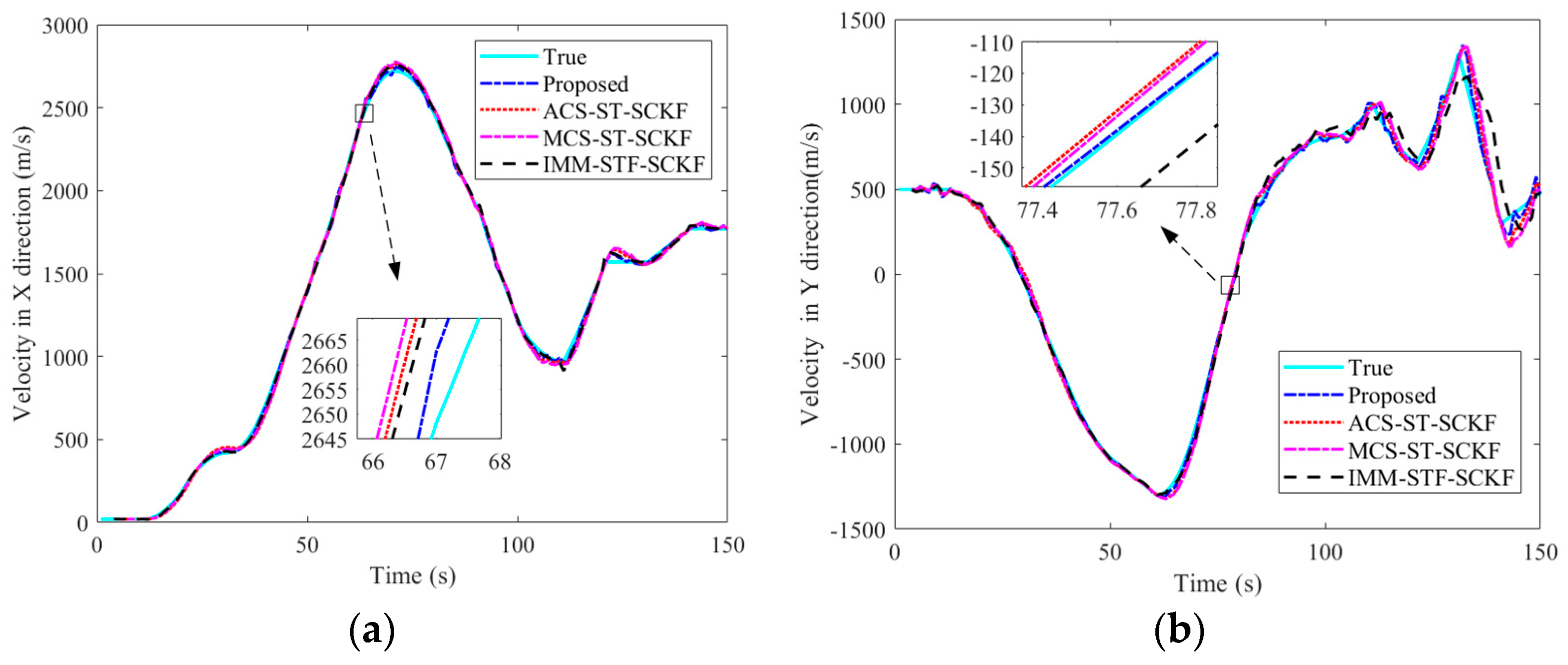
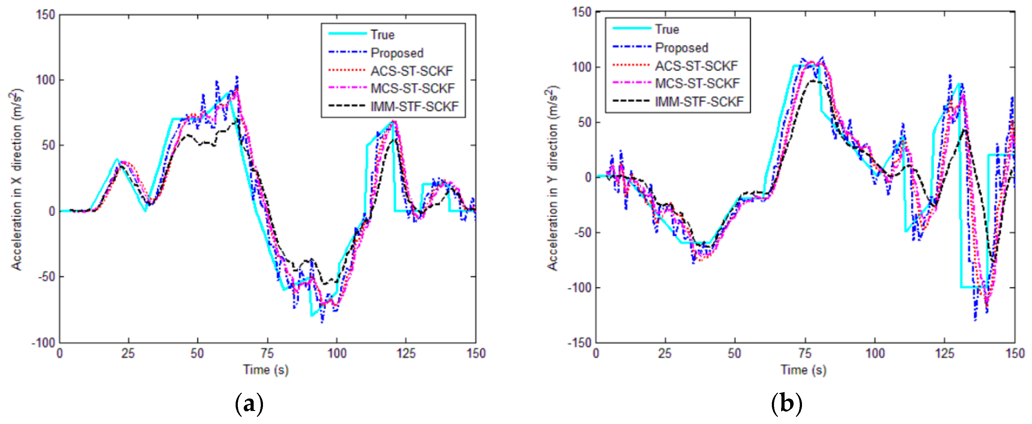
Figure 1, Figure 2 and Figure 3 show the true trajectory, velocity, acceleration, and estimates by the four filters, respectively. The target starts at point (0, 500), and the acceleration changes every 10 s. The division of maneuver states is shown in Table 2.
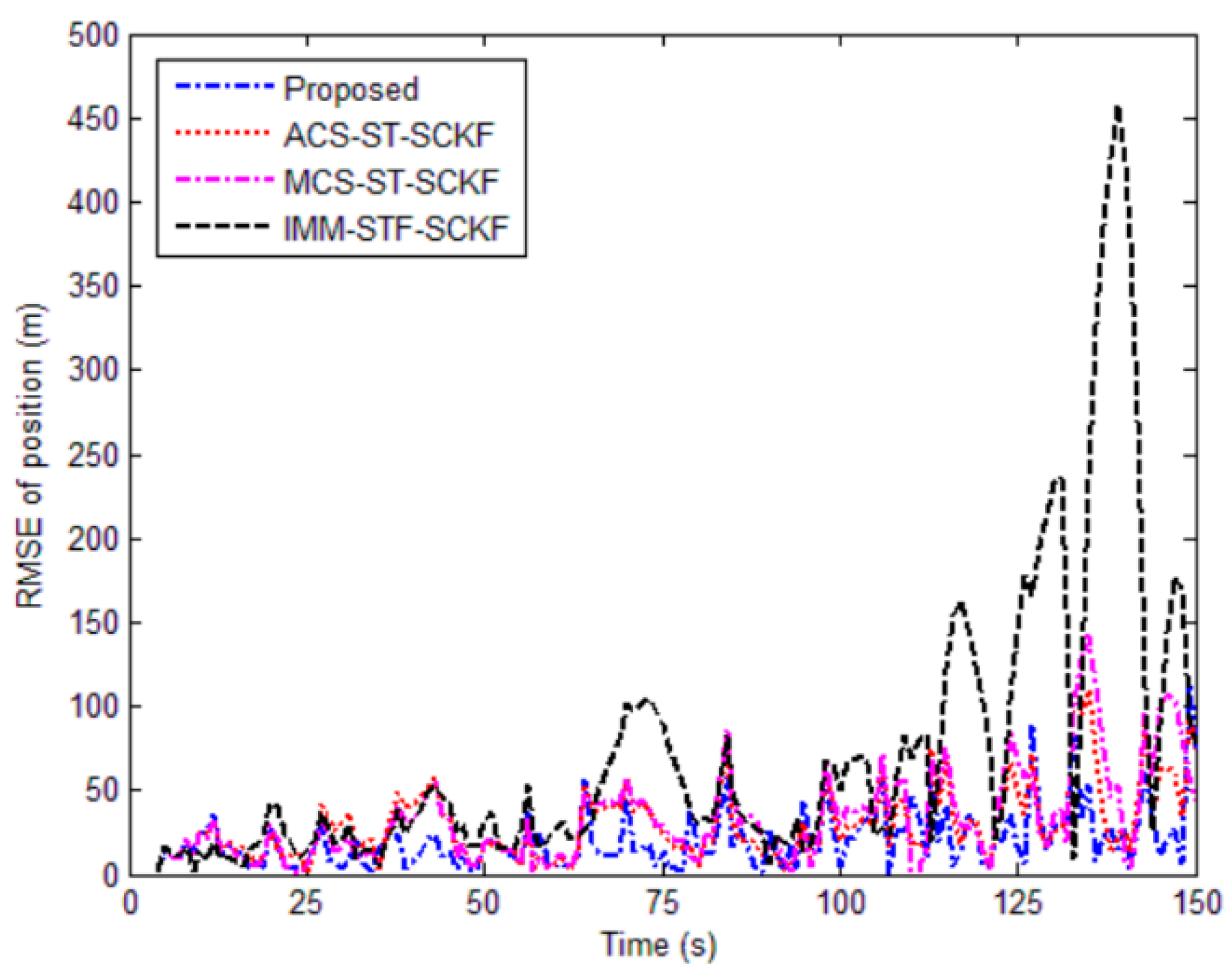
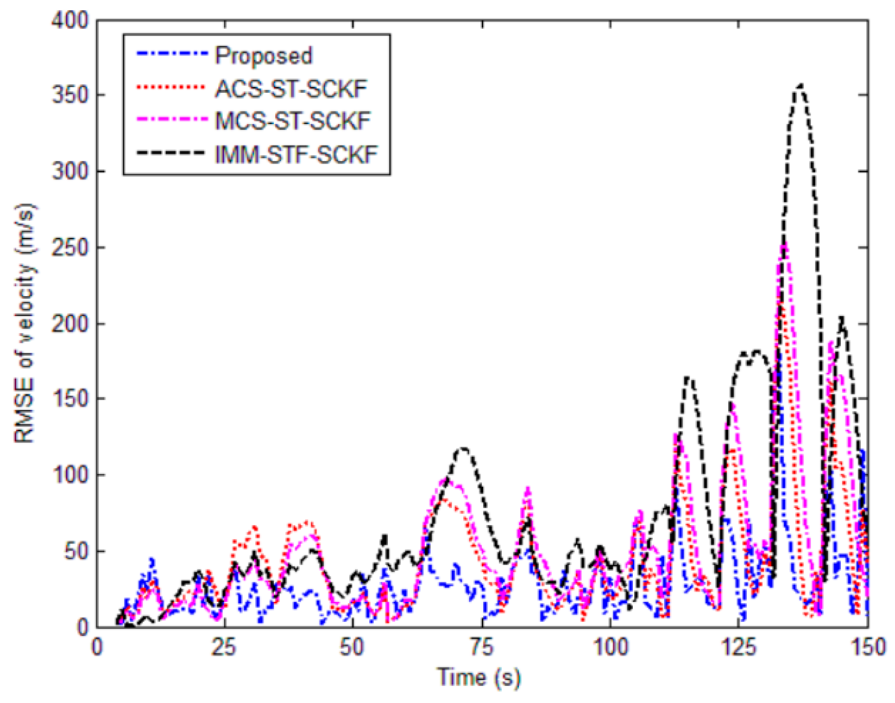
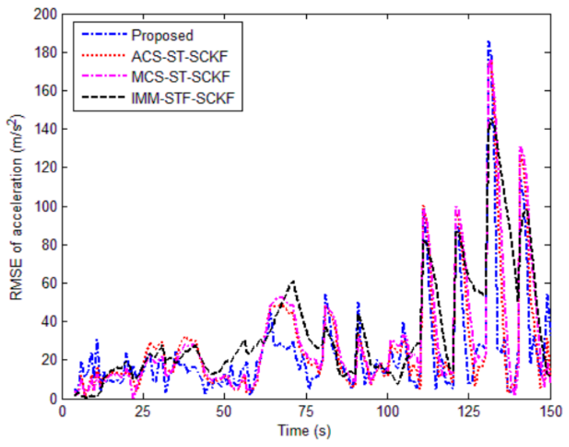
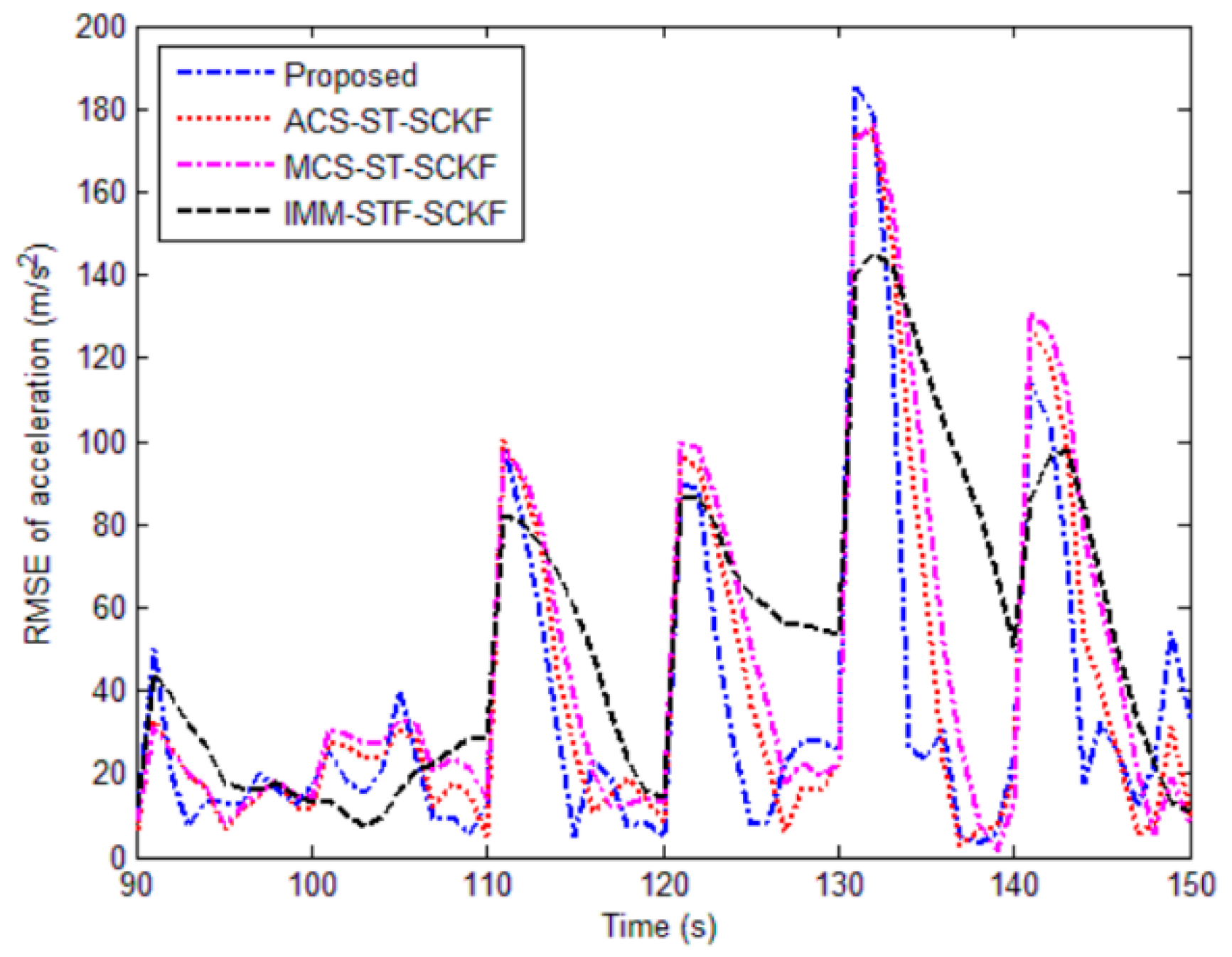
Figure 4, Figure 5 and Figure 6 show the RMSE of position, velocity, and acceleration, respectively. In the initial stage, i.e., 0–10 s, IMM-STF-SCKF performs the best among all the filters. That is because the CV model can well match the target motion during that period. However, as the target starts to maneuver, the IMM-STF-SCKF begins to show a highly degraded performance. Especially when faced with abrupt maneuvers, it usually shows the highest estimate error and the longest convergence time. Among the remaining filters, the proposed algorithm outperforms the other two. Though sometimes a little higher estimate error is performed when faced with severer shake of acceleration, (e.g., 90 s and 130 s, details are shown in Figure 7), the proposed filter converges in the quickest manner. The reason is that the proposed filter originates from the CA model, and the process noise is modeled by the colored noise. By contrast, the ACS-ST-SCKF and the MCS-ST-SCKF both augment the acceleration mean into the state vector. Such an augment results in a tardy reaction in the adaptation of maneuver motion.
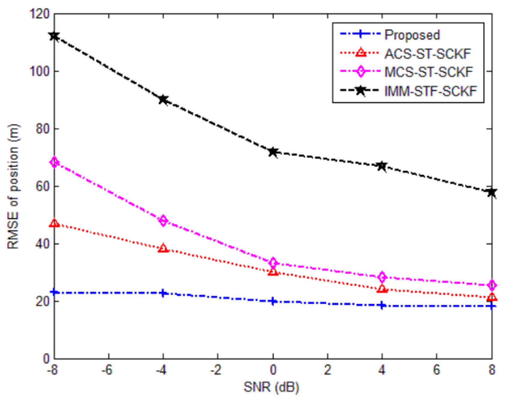
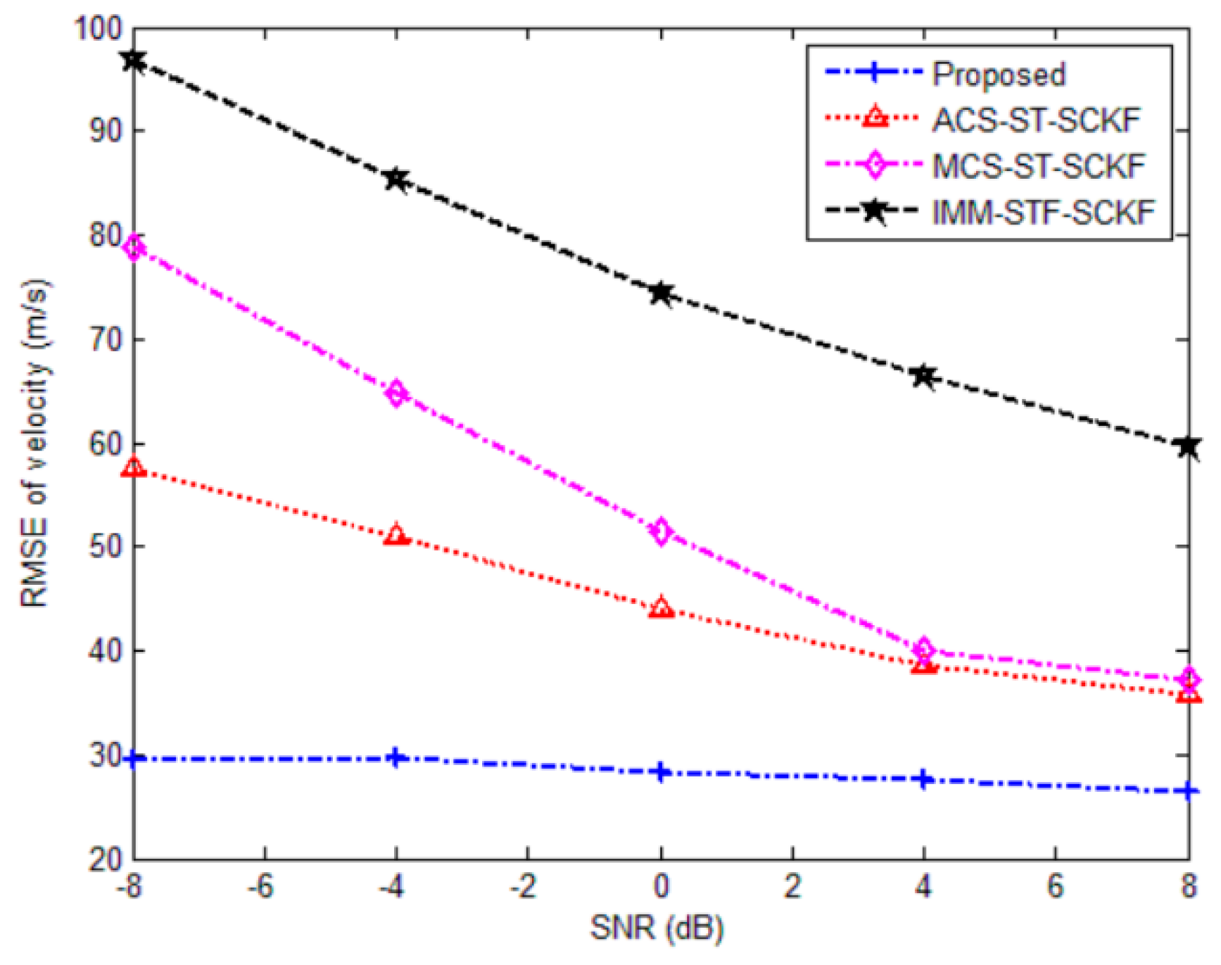
The MEs and runtime are given in Table 3, from which we can see that the proposed algorithm achieves the best performance and possesses the simplest structure. Specifically, when compared with the IMM-STF-SCKF, the proposed filter improves the position accuracy by 72.26%, velocity accuracy by 61.94%, and acceleration accuracy by 28.15%, respectively. Meanwhile, the runtime is decreased by 60.14%.
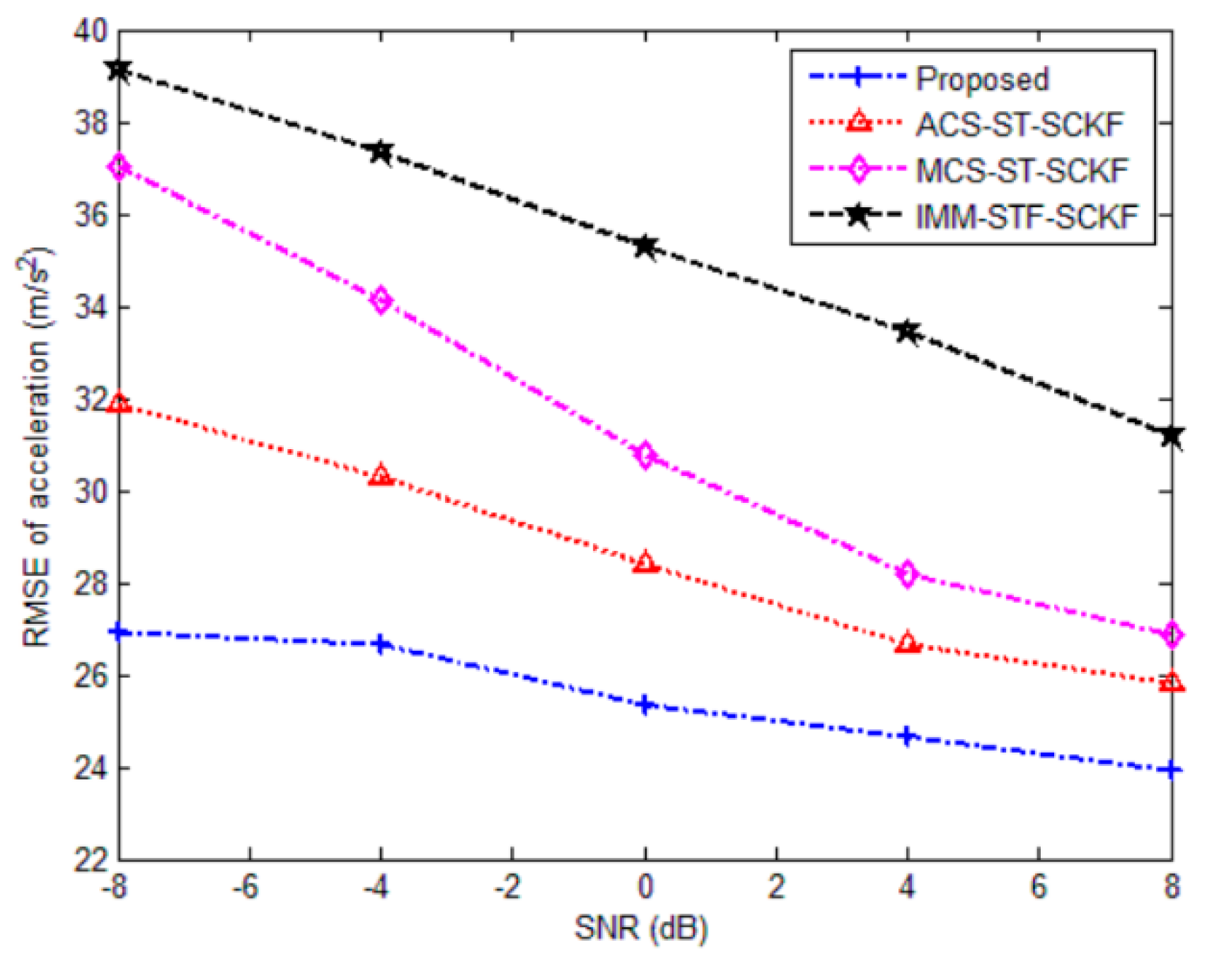
Additionally, we investigate the influence of signal-to-noise ratio (SNR) on the performance. Assume that Rk is obtained from 0 dB; the MEs in different SNRs are shown in Figure 8, Figure 9 and Figure 10. It can be seen that the performance of the proposed filter just changes a little when faced with different SNRs. By contrast, the tracking errors of the other three filters all decrease a lot as the SNR increases. However, the MEs of the proposed filter are always the smallest among all the filters, which verified its robustness.

5.2. Computational Complexity

Since Table 3 has shown the runtime of all the algorithms, the qualitative analysis of the computational complexity is given here. The four algorithms all adopt the ST-SCKF. Though the effective positions of the fading factor are different (the IMM-STF-SCKF adopts the traditional fading factor), the computational complexity is very close. As to the motion model, compared with the ACA model, two dimensions are augmented in the ACS model and the MCS model. However, in the ACA model, P k needs to be used for the calculation of P k + 1 . Therefore, the total computational complexity of the latter two filters is less than 1.3 times that of the ACA-ST-SCKF. As to the IMM model, three models with different complexities are adopted, and the interaction of multiple models also requires some computational burden. Hence, its computational complexity is less than three times that of the ACA-ST-SCKF.

6. Conclusions

A novel ST-SCKF based on the ACA model is proposed for the maneuvering target tracking problem. On the basis of the Taylor series expansion of acceleration, the relationship between the Jerk component and the velocity as well as acceleration is established. The state error covariance matrix is fully utilized to achieve the online adaptivity of the process noise. Thereby, the total self-adaptation of the proposed model is realized. Simulation results show that the proposed algorithm achieves better tracking precision while maintaining less runtime compared with the ACS-ST-SCKF, MCS-MSCKF, and IMM-STF-SCKF.
Future works include the incorporation of the maneuvering target tracking problem into more tasks, such as classification [26] and rejecting clutter [27,28].

Author Contributions

Conceptualization, W.F., H.Z.; funding acquisition, J.X. and W.F.; methodology, J.X., J.H., and Z.L.; validation, Z.L.; writing—original draft, J.H. All authors have read and agreed to the published version of the manuscript.

Funding

This research was funded by the Youth Talent Lifting Project of the China Association for Science and Technology, grant number 2021-JCJQ-QT-018 (W.F.), and also funded in part by the Shaanxi Association of Science and Technology Youth Talent Support Program Project, grant number 20230137 (H.Z.).

Data Availability Statement

The original contributions presented in this study are included within the article. further inquiries can be directed to the corresponding authors.

Conflicts of Interest

The authors declare that we do not have any commercial or associative interest that represents conflicts of interest in connection with the work submitted.

References

  1. Li, X.R.; Jilkov, V.P. Survey of maneuvering target tracking. Part I: Dynamic models. IEEE Trans. Aerosp. Electron. Syst. 2003, 39, 1333–1363. [Google Scholar]
  2. Singer, R.A. Estimating optimal tracking filter performance for manned maneuvering targets. IEEE Trans. Aerosp. Electron. Syst. 1970, 6, 473–483. [Google Scholar] [CrossRef]
  3. Zhou, H.; Kumar, K.S.P. A ‘current’ statistical model and adaptive algorithm for estimating maneuvering targets. AIAA J. Guid. 1984, 7, 596–602. [Google Scholar] [CrossRef]
  4. Kishore, M.; Pravas, R.M. A Jerk model for tracking highly maneuvering targets. IEEE Trans. Aerosp. Electron. Syst. 1997, 3, 1094–1105. [Google Scholar]
  5. Zhang, H.; Xie, J.; Ge, J.; Lu, W.; Liu, B. Strong tracking SCKF based on adaptive CS model for manoeuvring aircraft tracking. IET Radar Sonar Navig. 2018, 12, 742–749. [Google Scholar] [CrossRef]
  6. Zhang, H.; Xie, J.; Ge, J.; Lu, W.; Zong, B. Adaptive strong tracking square-root cubature Kalman filter for maneuvering aircraft tracking. IEEE Access 2018, 6, 10052–10061. [Google Scholar] [CrossRef]
  7. Liu, W.; Li, Y.; Cui, L. Adaptive strong tracking algorithm for maneuvering targets based on current statistical model. Syst. Eng. Electron. 2011, 33, 1937–1940. [Google Scholar]
  8. Yang, Y.; Fan, X.; Zhuo, Z. AFAKF for manoeuvring target tracking based on current statistical model. IET Sci. Meas. Technol. 2016, 10, 637–643. [Google Scholar] [CrossRef]
  9. Wang, M.; Wang, H. An adaptive attitude algorithm based on a current statistical model for maneuvering acceleration. Chin. J. Aeronaut. 2017, 30, 426–433. [Google Scholar] [CrossRef]
  10. Chen, L.; Gong, X.; Shi, H.; Yang, J. Maneuvering frequency adaptive algorithm of maneuvering target tracking. In Proceedings of the Fourth International Conference on Intelligent Control and Information Processing, Beijing, China, 9–11 June 2013; pp. 455–458. [Google Scholar]
  11. Zhu, D.; Chen, K.; Gen, W. A new adaptive filtering algorithm based on the current statistical model. In Proceedings of the Fifth International Conference on Intelligent Human-Machine Systems and Cybernetics, Hangzhou, China, 26–27 August 2013; pp. 3–6. [Google Scholar]
  12. Julier, S.J.; Uhlmann, J.K.; Durrant-Whyte, H.F. A new method for the nonlinear transformation of means and covariances in filters and estimators. IEEE Trans. Autom. Control 2000, 45, 477–482. [Google Scholar] [CrossRef]
  13. Jia, B.; Xin, M.; Cheng, Y. Sparse-grid quadrature nonlinear filtering. Automatica 2012, 48, 327–341. [Google Scholar] [CrossRef]
  14. Arasaratnam, I.; Haykin, S. Cubature Kalman filters. IEEE Trans. Autom. Control 2009, 54, 1254–1269. [Google Scholar] [CrossRef]
  15. Jazwinski, H. Filtering for nonlinear dynamic systems. IEEE Trans. Autom. Control 1996, 11, 765–766. [Google Scholar] [CrossRef]
  16. Zhou, D.H.; Sun, Y.X.; Xi, Y.G.; Zhang, Z.J. Extension of friedland’s separate bias estimation to randomly time-varying bias of nonlinear systems. IEEE Trans. Autom. Control 1993, 38, 1270–1273. [Google Scholar] [CrossRef]
  17. Zhang, G.; Zhang, X.; Zeng, L.; Dai, S.; Zhang, M.; Lian, F. Filtering in Triplet Markov Chain Model in the Presence of Non-Gaussian Noise with Application to Target Tracking. Remote Sens. 2023, 15, 5543. [Google Scholar] [CrossRef]
  18. Shan, C.; Zhou, W.; Jiang, Z.; Shan, H. A new Gaussian approximate filter with colored non-stationary heavy-tailed measurement noise. Digit. Signal Process. 2022, 122, 103358. [Google Scholar] [CrossRef]
  19. Huang, Y.; Zhang, Y.; Li, N.; Wu, Z.; Chambers, J.A. A Novel Robust Student’s t-Based Kalman Filter. IEEE Trans. Aerosp. Electron. Syst. 2017, 53, 1545–1554. [Google Scholar] [CrossRef]
  20. Huang, Y.; Zhang, Y.; Shi, P.; Wu, Z.; Qian, J.; Chambers, J.A. Robust Kalman Filters Based on Gaussian Scale Mixture Distributions With Application to Target Tracking. IEEE Trans. Syst. Man Cybern. Syst. 2019, 49, 2082–2096. [Google Scholar] [CrossRef]
  21. Huang, Y.; Zhang, Y.; Shi, P.; Chambers, J. Variational Adaptive Kalman Filter With Gaussian-Inverse-Wishart Mixture Distribution. IEEE Trans. Autom. Control 2021, 66, 1786–1793. [Google Scholar] [CrossRef]
  22. Xue, C.; Huang, Y.; Zhu, F.; Zhang, Y.; Chambers, J.A. An Outlier-Robust Kalman Filter With Adaptive Selection of Elliptically Contoured Distributions. IEEE Trans. Signal Process. 2022, 70, 994–1009. [Google Scholar] [CrossRef]
  23. Zhu, F.; Huang, Y.; Xue, C.; Mihaylova, L.; Chambers, J. A Sliding Window Variational Outlier-Robust Kalman Filter Based on Student’s t-Noise Modeling. IEEE Trans. Aerosp. Electron. Syst. 2022, 58, 4835–4849. [Google Scholar] [CrossRef]
  24. Pan, Q.; Liang, Y.; Yang, F.; Cheng, Y. Modern Aircraft Tracking and Information Fusion, 1st ed.; National Defense Industry Press: Beijing, China, 2009. [Google Scholar]
  25. Han, B.; Huang, H.; Lei, L.; Huang, C.; Zhang, Z. An Improved IMM Algorithm Based on STSRCKF for Maneuvering Target Tracking. IEEE Access 2019, 7, 57795–57804. [Google Scholar] [CrossRef]
  26. Wang, L.; Zhan, R.; Liu, S.; Zhang, J.; Zhuang, Z. Joint tracking and classification of multiple extended targets via the PHD filter and star-convex RHM. Digit. Signal Prog. 2021, 111, 102961. [Google Scholar] [CrossRef]
  27. Ding, L.; Xu, X.; Cao, Y.; Zhai, G.; Yang, F.; Qian, L. Detection and tracking of infrared small target by jointly using SSD and pipeline filter. Digit. Signal Prog. 2021, 110, 102949. [Google Scholar] [CrossRef]
  28. Luo, Q.; Gao, Z.; Xie, C. Improved GM-PHD filter based on threshold separation clusterer for space-based starry-sky background weak point target tracking. Digit. Signal Prog. 2020, 103, 102766. [Google Scholar] [CrossRef]
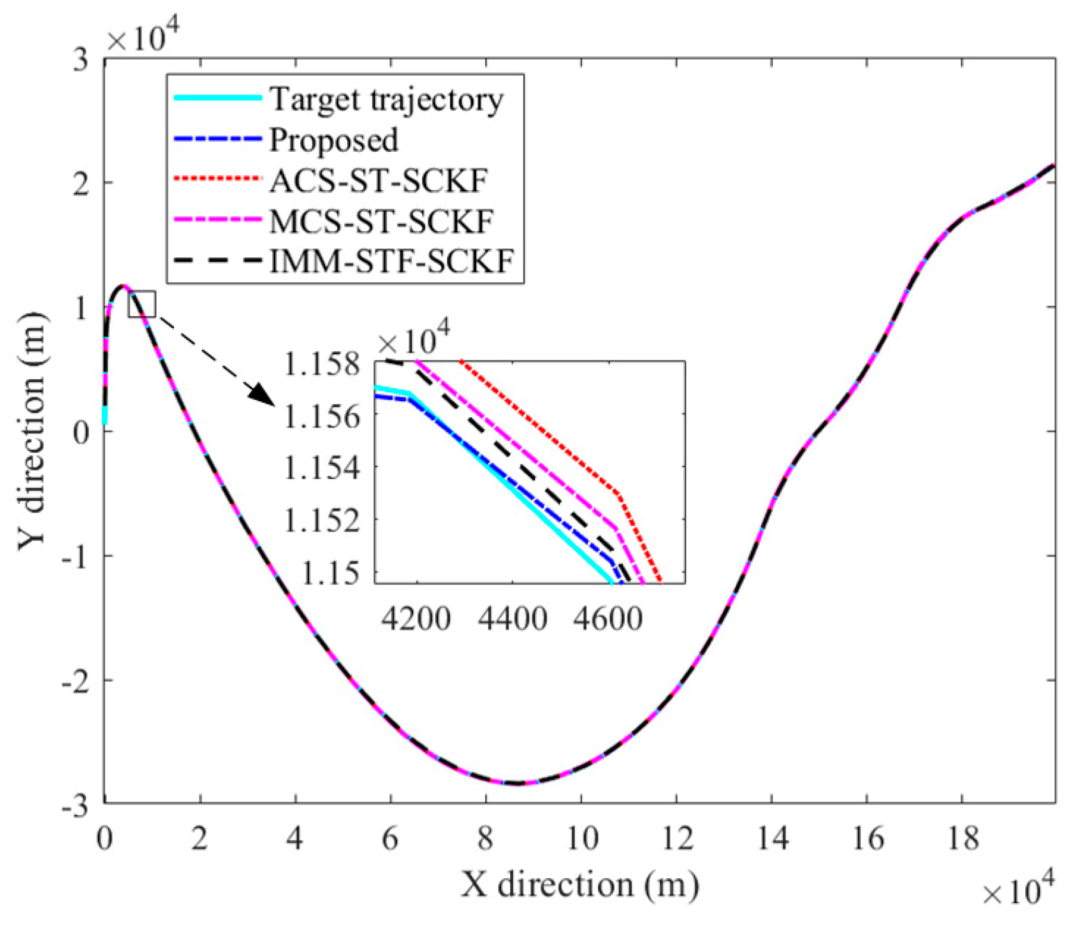
Figure 1. Trajectory and estimate.
Remotesensing 17 00850 g001
Figure 2. Velocity and estimate: (a) X direction and (b) Y direction.
Remotesensing 17 00850 g002
Figure 3. Acceleration and estimate: (a) X direction and (b) Y direction.
Remotesensing 17 00850 g003
Figure 4. RMSE of position.
Remotesensing 17 00850 g004
Figure 5. RMSE of velocity.
Remotesensing 17 00850 g005
Figure 6. RMSE of acceleration.
Remotesensing 17 00850 g006
Figure 7. RMSEs of acceleration in 90 s–150 s.
Remotesensing 17 00850 g007
Figure 8. MEs of positions in different SNRs.
Remotesensing 17 00850 g008
Figure 9. MEs of velocities in different SNRs.
Remotesensing 17 00850 g009
Figure 10. MEs of accelerations in different SNRs.
Remotesensing 17 00850 g010
Table 1. Description of parameters.
ParametersDescription
F k state transition matrix
U k acceleration input matrix
a ¯ k input acceleration mean
h nonlinear transformation
w k process noise, w k N ( 0 , Q k ) , i.e., the Gaussian distribution with zero mean and covariance
Q k Q k = 2 α σ a 2 q cs
q cs symmetric matrices of fixed form
α maneuvering frequency
v k measurement noise, v k N ( 0 , R k )
Table 2. Division of maneuver states.
Maneuver DescriptionTime (s)
Steady state0~10, 130~140, 140~150
Weak maneuver50~60, 60~70, 70~80, 80~90, 90~100, 100~110, 110~120, 120~130
Continuous maneuver0~50
Abrupt maneuver10, 20, 30, 40, 50, 60, 70, 80, 90, 100, 110, 120, 130, 140
Table 3. MEs and runtime.
AlgorithmsMean Error (ME)Mean Runtime (s)
Position (m)Velocity (m/s)Acceleration (m/s2)
Proposed19.886528.356225.33830.0460
ACS-ST-SCKF29.911244.051628.37460.0588
MCS-ST-SCKF33.142851.405630.73850.0596
IMM- STF-SCKF71.687474.430035.26350.1154
Disclaimer/Publisher’s Note: The statements, opinions and data contained in all publications are solely those of the individual author(s) and contributor(s) and not of MDPI and/or the editor(s). MDPI and/or the editor(s) disclaim responsibility for any injury to people or property resulting from any ideas, methods, instructions or products referred to in the content.