Unsupervised SAR Image Change Detection Based on Curvelet Fusion and Local Patch Similarity Information Clustering

Abstract

Change detection for synthetic aperture radar (SAR) images effectively identifies and analyzes changes in the ground surface, demonstrating significant value in applications such as urban planning, natural disaster assessment, and environmental protection. Since speckle noise is an inherent characteristic of SAR images, noise suppression has always been a challenging problem. At the same time, the existing unsupervised deep learning-based methods relying on the pseudo labels may lead to a low-performance network. These methods are high data-dependent. To this end, we propose a novel unsupervised change detection method based on curvelet fusion and local patch similarity information clustering (CF-LPSICM). Firstly, a curvelet fusion module is designed to utilize the complementary information of different difference images. Different fusion rules are designed for the low-frequency subband, mid-frequency directional subband, and high-frequency subband of curvelet coefficients. Then the proposed local patch similarity information clustering algorithm is used to classify the image pixels to output the final change map. The pixels with similar structures and the weight of spatial information are incorporated into the traditional clustering algorithm in a fuzzy way, which greatly suppresses the speckle noise and enhances the structural information of the changing area. Experimental results and analysis on five datasets verify the effectiveness and robustness of the proposed method.

1. Introduction

The change detection task involves analyzing and comparing images acquired at different times in the same location, identifying the changed areas and the unchanged areas, and ultimately representing the result as a binary image. Because synthetic aperture radar (SAR) has the characteristics of all-day and all-weather coverage and strong penetration [1,2], it is currently widely used in land cover, disaster monitoring and assessment, urban planning, etc. [3,4]. Currently, many SAR satellites are able to obtain many multi-temporal SAR images. Due to the high-resolution imaging technology of the SAR system [5,6], SAR images are characterized by high resolution, high-repeat cycle, and wide coverage. It is very important and meaningful to propose a new intelligent remote sensing image processing algorithm to simply, quickly, and accurately analyze SAR imagery information.

Due to the special imaging system of SAR, SAR images inevitably have speckle noise. Overcoming the influence of speckle noise on images is very challenging. A large number of experts and scholars have conducted many studies and contributions in this regard [7,8,9,10]. At the same time, excessive denoising will also lead to the loss of image details. How to strike a balance between denoising and detail preservation is a problem worth studying. For unsupervised change detection methods, denoising is particularly important. Unsupervised SAR image change detection is usually divided into the following processes: first, image preprocessing, then, difference image generation, and finally, difference image analysis. Image preprocessing primarily involves image registration and geometric correction [11]. The generation of difference images generally directly reflects the quality of subsequent difference image analysis results, so a large number of experts and scholars are committed to studying better difference image generation methods [12,13,14]. The difference image contains many potential change areas. The purpose of difference image analysis is to find out the areas that are most likely to have changed and the areas that are most likely not to have changed. Since the noise model of SAR images is a multiplicative noise model, the logarithmic ratio (LR) operator [15] converts multiplicative noise into additive noise, thus preserving the background and emphasizing the changed areas. The mean ratio operator [16] takes average gray value of the pixel’s neighborhood, which has a good suppression effect on speckle noise, but has poor suppression in areas with severe noise. Gong et al. designed a local similarity measurement to judge the similarity of pixel patches in [17]. Multi-difference image fusion is used to obtain different information from different difference images, and uses complementary information to form a better image, which provides reliable information for subsequent difference image analysis. Zheng et al. performed parameter weighting on different difference images in [18]. Peng et al. proposed a visual saliency difference image generation method [19], which is represented by multi-dimensional difference features and fuses the difference images of three different algorithms for feature fusion. These fused difference images usually show a good denoising performance. However, combining different difference images in the spatial domain usually only represents the image intensity information, and often cannot represent the image texture and edge well. Therefore, many experts and scholars later tried to study the fusion difference image in the frequency domain. Hou et al. used discrete wavelet transform to fuse complementary information in high and low frequency bands of different difference images in [20], and used contourlet transform to set the threshold on the high frequency band coefficients of the fused difference image for denoising. Ma et al. proposed a wavelet-based fusion difference image [21], which combines the advantages of mean ratio operator and LR operator. Zhang et al. proposed to use contourlet transform to fuse different difference images in [22]. Contourlet can effectively capture the multi-scale features and provide good directionality, so that it can better represent the image features with edge and curve structures. However, these methods do not provide a better division and fusion of frequency domain information.

Difference image analysis is used to classify pixels into two categories, and the purpose of this is to divide changed areas. Thresholding and clustering are the most popular unsupervised approaches. The threshold method selects a specific threshold to divide the image into several meaningful areas. The selection of the optimal threshold requires the establishment of a model to fit the conditional distribution of changed and unchanged pixels [23,24]. In addition, the clustering algorithm is more flexible and has a better generalization ability, does not require model building, and is more robust to noise. Fuzzy clustering is an image segmentation algorithm because fuzzifying the membership matrix can preserve more information of the pixels. Fuzzy c-means clustering (FCM) [25] is the most classic clustering algorithm, but it is sensitive to noise because it ignores contextual information. Subsequently, many experts and scholars have proposed various variants of FCM. Krinidis et al. considered local information based on FCM in [26], which made the fuzzy local information c-means (FLICM) cluster algorithm more robust. Subsequently, an improved FLICM algorithm was proposed in [27], which expanded the neighborhood size to $5\times 5$, reduced the interference of isolated noise on FLICM, and made the calculation of the membership matrix more accurate. Subsequently, many experts and scholars improved the FCM algorithm to detect changing images in [28,29]. The FLICM algorithm has a good performance in suppressing speckle noise, its framework is applicable for detecting SAR image. For FLICM, we add local direction weights and spatial weights into the fuzzy factor, which can effectively segment the image when the change area is large and complex. The FLICM algorithm is supplemented with local similar patch information and spatial weighted information to improve the algorithm’s denoising performance.

Deep learning is becoming increasingly popular and efficient, and training deep learning models has been widely used in difference image analysis. These models usually use unsupervised methods to extract labeled samples, and the trained models are mainly used as classifiers to identify potential change pixels. Cui et al. proposed a hierarchical clustering method for pixel pre-classification in [30], and finally trained the network to perform binary classification on uncertain pixels. Gao et al. proposed a PCANet to analyze SAR image in [31]. The convolutional neural network (CNN) is widely used in the vision field, and many CNN-based variants are designed for SAR image change detection. Gao et al. combined wavelet and convolutional neural network in [32]. Zhang et al. performed a threshold analysis on the difference image in [33] by minimizing the histogram fitting error and then fed the difference image into CNN. Zhang et al. combined CNN and Transformer in both series and parallel modes [34], enhancing the connection between features. Recently, Chen et al. proposed an efficient spatial-frequency network in [35], which extracts noise-robust features in both spatial and frequency domains and significantly improves computational efficiency. Dong et al. proposed a new dynamic bilinear fusion network (DBFNet) [36] to capture the dependency relationship between spatio-temporal features. Xie et al. proposed a wavelet-based bi-dimensional aggregation network (WBANet) [37], which introduced wavelet in the self-attention block. Deep neural networks are now commonly used in various fields [38,39]. Gong and Zhao et al. have proposed an end-to-end deep neural network to directly classify the original image in [40,41] without generating difference images. Dong et al. designed a shearlet denoising layer to enhance feature extraction, a deep shearlet convolutional neural network is proposed in [42]. Zhang et al. designed deep convolutional generative adversarial networks to add pseudo labels to solve the sample difference problem in [43]. These network models usually achieve excellent performance, but at the same time, the complex architecture and randomness of sample selection are also very important to consider.

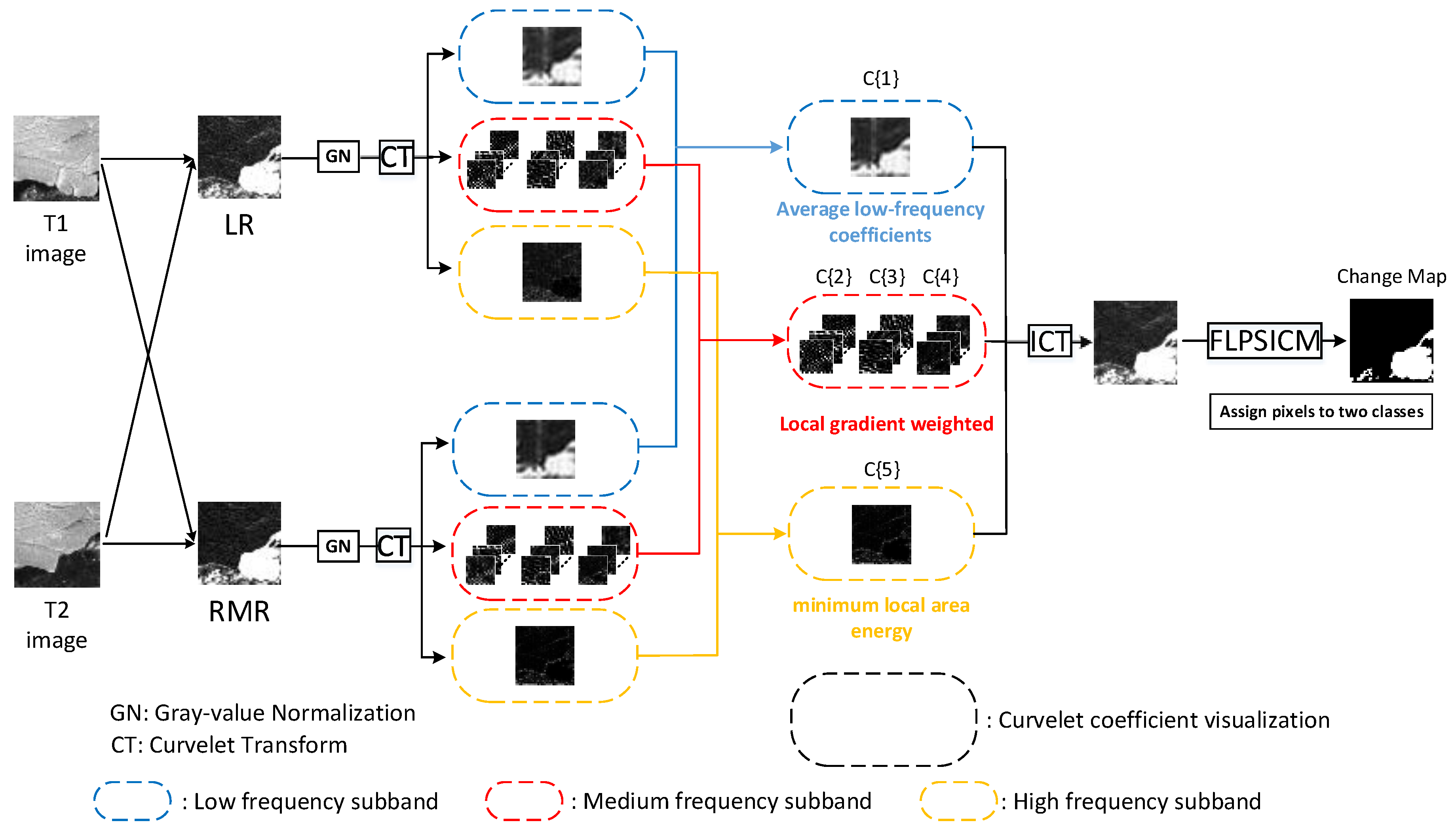
Until now, deep learning has made significant progress and success in SAR imagery change detection, but sample uncertainty and complex architecture are still difficult to solve. In this paper, we focus on generating difference images with more detailed information while suppressing noise in SAR images. First of all, we need to get a better difference image. We choose curvelet fusion strategy and use the complementary information of different operator images to form a fusion image, which provides powerful help for subsequent difference image analysis. The curvelet transform (CT) is used to decompose the difference image in the frequency domain, dividing the frequency domain information of different scales into low, medium, and high frequency components. Different fusion rules are designed for the three levels of information. Then, the fused difference image is obtained through inverse transformation. A clustering method is used for difference image analysis, local patch similarity information and local spatial weighting are introduced into the FLICM clustering algorithm to enhance the algorithm’s robustness to noise. The improved algorithm framework fuzzy local patch similarity information c-means (FLPSICM) is very suitable for detecting changed SAR images. Combining curvelet fusion and clustering, we propose a change detection framework for SAR images based on curvelet fusion and local patch similarity information clustering (CF-LPSICM), as shown in Figure 1. The main contributions of this paper are as follows:

(1) A novel unsupervised method framework is proposed for SAR imagery change detection.

(2) A curvelet fusion model based on local gradient weighting and energy is designed to generate high-quality difference images, effectively utilizing the complementary information of the two difference images.

(3) A new clustering algorithm combining local patch similarity information and spatial weighting is proposed, which suppresses noise while enhancing pixel structure information, and the unsupervised analysis method is more flexible and faster.

(4) The experimental results are compared in four different scenes, which proves that CF-LPSICM method has the most advanced performance and can accurately detect the changed area.

The rest of this article is organized as follows. Section 2 details the proposed approach, Section 3 shows the experiments and analysis, and Section 4 concludes.

2. Method

The framework of the proposed method CF-LPSICM is shown in Figure 1. This method can be divided into the following steps: difference image generation, curvelet fusion, local patch similarity information clustering and output detection results.

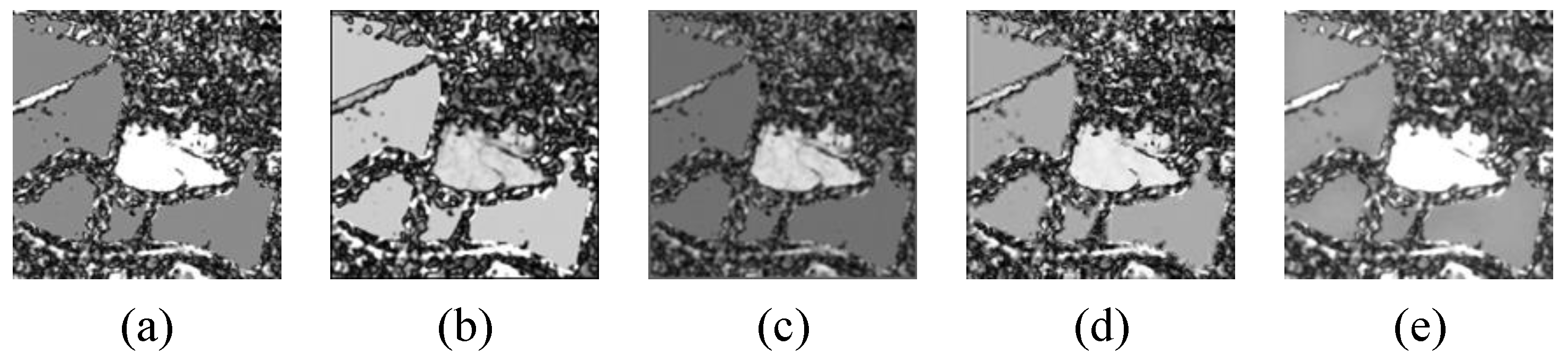
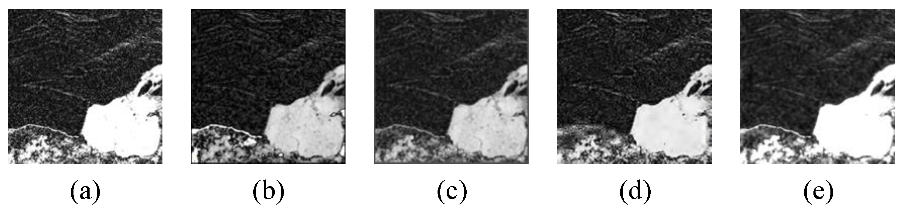
Firstly, in order to fully utilize complementary information, the LR operator image and the ratio–mean ratio (RMR) operator image [44] are used as fusion images. The LR operator image retains a lot of background information, and the RMR operator image suppresses noise. Apply curvelet transform to the difference images. Then, the frequency domain information is hierarchically divided and utilized, the fusion schemes of the high-frequency, medium-frequency and low-frequency sub-band coefficients after curvelet transform are designed respectively. The low-frequency sub-band coefficients represent background contours, which should be retained as much as possible. The mid-frequency sub-band coefficients represent image textures, which should be highlighted. The high-frequency sub-band coefficients represent noise, which should be suppressed. Finally, in the step of clustering analysis of difference images, in order to effectively suppress speckle noise in SAR images and enhance the structural information of the changed area, local spatial weight and local patch similarity measurement are introduced into the fuzzy factor of the FLICM algorithm. The details of difference image generation, curvelet fusion difference image and local patch similarity information cluster are reported in Section 2.1–Section 2.3.

2.1. Difference Image Generation

Since SAR images have multiplicative speckle noise, noise greatly affects the results. The mean ratio algorithm can suppress the speckle noise in the background information and play a role in spatial filtering, but it is not effective in suppressing areas with severe noise. Xuan et al. proposed the RMR operator difference image [44], which multiplied the ratio operator with the mean ratio operator, greatly improving a suppression effect on severe noise areas. The LR operator is a nonlinear algorithm that retains most background information. In the experiment, the LR and RMR operators were used to generate difference images. The LR operator plays a role in retaining details, and the RMR operator plays a role in denoising. The formulas of the two operators are as follows:

$$I_l=\left|log{\displaystyle \frac{I_2(x,y)}{I_1(x,y)}}\right|,$$

(1)

$$\begin{array}{c}\hfill I_{rmr}=\left|1-min\left\{{\displaystyle \frac{{\mu }_1(x,y)}{{\mu }_2(x,y)}},{\displaystyle \frac{{\mu }_2(x,y)}{{\mu }_1(x,y)}}\right\}\right|\\ \hfill \times \left|{\displaystyle \frac{I_1(x,y)-I_2(x,y)}{I_1(x,y)+I_2(x,y)}}\right|\end{array},$$

(2)

where $I_1$ and $I_2$ are two SAR images gray-values of the same size at different times after correction and registration, ${\mu }_1$ and ${\mu }_2$ are the average gray values of pixels in the neighborhood windows centered at the coordinates in the two images. Then normalize the two images to regularize gray value.

2.2. Curvelet Fusion Difference Image

Curvelet transform [45] is an image decomposition method developed based on wavelet transform. The curvelet transform is anisotropic and multi-directional. The coefficients decomposed by the curvelet transform can contain more original image information than the coefficients decomposed by the wavelet transform. CT is sensitive to image edges and textures. It can represent image texture information at different scales through a small number of sparse non-zero coefficients. In this paper, we adopt the second-generation curvelet transform [46], which avoids ridgelet calculation compared with the first-generation transform and is multi-scale and multi-directional. The algorithm is simpler and faster. First, the image is subjected to a two-dimensional Fast Fourier Transform (FFT), and then the two-dimensional Fourier frequency domain plane is divided using a wedge basis. Appropriate curvelet coefficients are selected for all bases at each scale j and direction l, and finally these bases are inversely transformed by FFT.

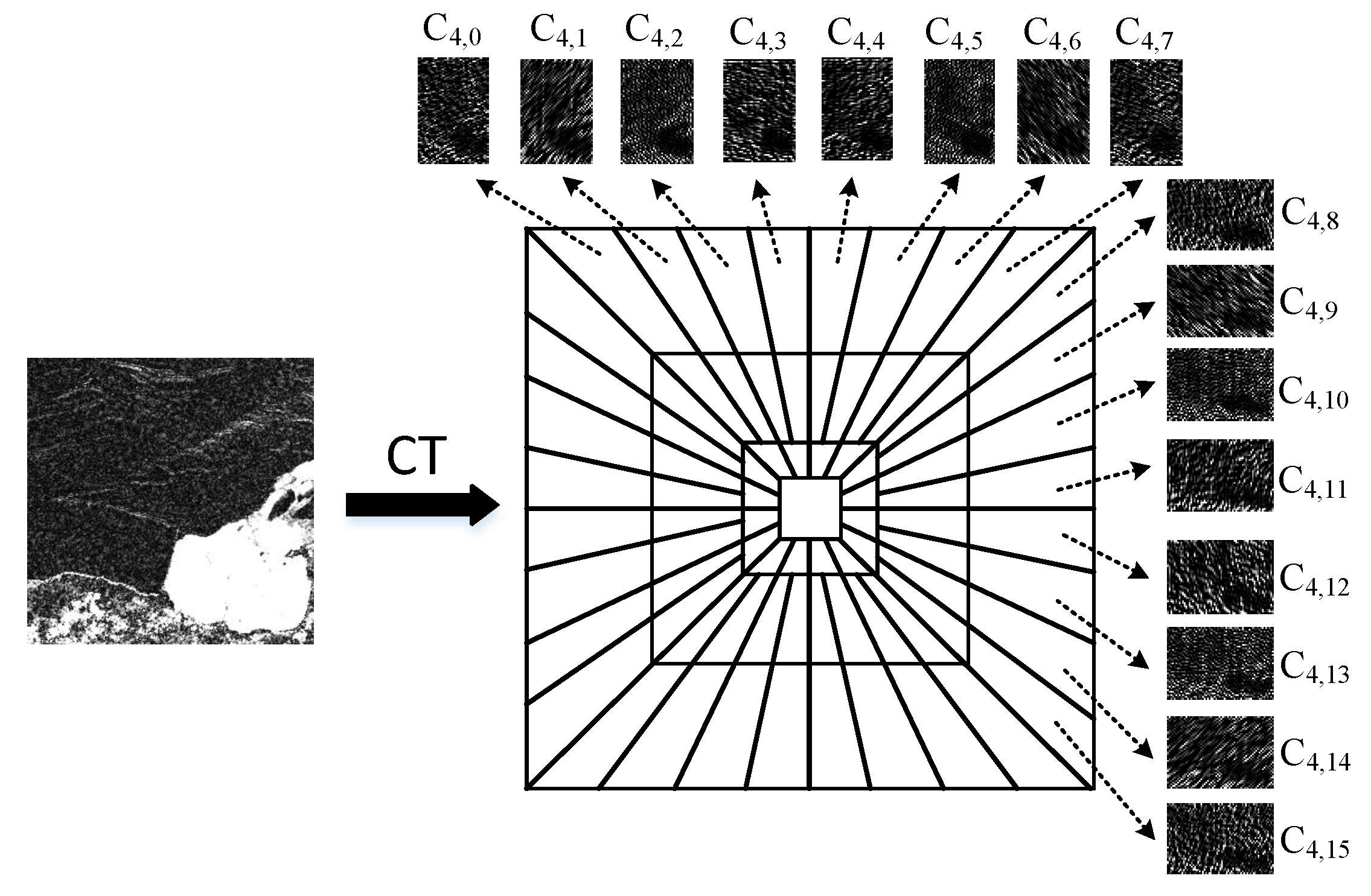
The image frequency domain spatial distribution diagram is shown in Figure 2 after the image is subjected to discrete curvelet transform. The surrounding small images are visualizations of the outermost curvelet coefficients when the decomposition scale is 4. The curvelet transform evenly divides the frequency domain into rings containing different directions, it can be seen that as the decomposition scale increases, the image has more decomposition directions in the frequency domain, and texture information in more directions is extracted. Curvelets provide a mathematical framework that is well suited for representing objects that display smoothness with discontinuities in curves, such as images with edges. This is well suited for representing the appearance of changing areas in SAR images.

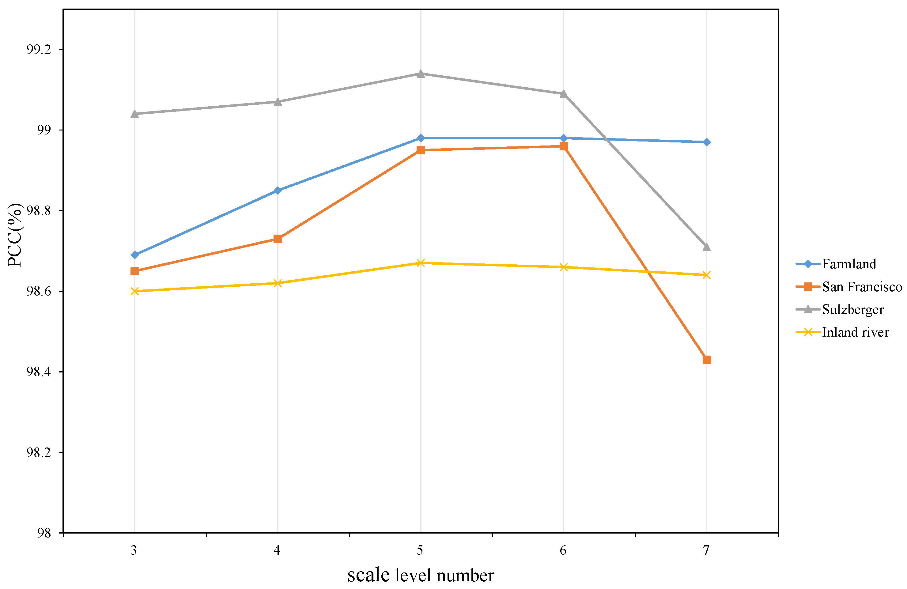
It is very important to choose a fusion method to fuse the high, medium, and low frequency information of the image. The decomposition scale for the image after the curvelet transform varies with the image size. The default decomposition scale number calculation formula proposed in [46] is ${log}_2(min(H,W))-3$, rounded up, H and W are the height and width of the image. The image after curvelet transformation has strong anisotropy at the fine level and can express the texture and edges of the image in different directions well. The image is transformed by curvelet transform to get the coefficient matrix C{j}{l} in different directions at different scales, where j represents the scale and l represents the direction at this scale. For example, if the LR operator difference image is transformed by curvelet transform, the decomposition scale is 5, the innermost and outermost layers are coefficient matrices C{1}, C{5} composed of low-frequency coefficients and high-frequency coefficients, and the number of directions of C{2} C{3} C{4} at the 2nd, 3rd, and 4th scales are 16, 32, and 32 respectively. The fusion schemes are shown in Figure 1. First, the two different difference images are decomposed by curvelet transform to generate frequency domain sub-band coefficients at different scales. Different fusion rules are designed for the sub-band coefficients at different scales of the image. All scales are divided. The coefficients at the first scale show the overall contour information, that is, low-frequency information. The sub-band coefficients at the second to fourth scales show more of the texture of the image, and the edges also have contour information, so they are set to medium-frequency information. The coefficients of the last scale show the edges of the image, but also contain a lot of speckle noise, which is high-frequency information. Three different fusion rules are designed for the low, medium and high frequency domain information. In the following, C_l represents the sub-band coefficient of the LR difference image, and C_m represents the sub-band coefficient of the RMR difference image.The default decomposition scale level is set to 5.

a. First, for the low-frequency sub-band, that is, the coefficients at the first scale, the following fusion rules are proposed as follows:

$$C_F\left\{1\right\}={\displaystyle \frac{C_l\left\{1\right\}+C_m\left\{1\right\}}{\alpha }},$$

(3)

a similar method to averaging is adopted, and $\alpha$ is set to 1.7, which retains the most background information. Where ${\mathit{C}}_{\mathit{F}}$ represents the fused coefficient tensor.

b. For the fusion of medium frequency sub-bands, the medium frequency coefficients usually depict the texture and edge information in the image and reflect the clarity of the image. The gradient of image pixels reflects the image sharpness. The larger the gradient, the sharper the image, containing more texture information, and less affected by noise and loss of details. The image gradient is calculated by median-value difference, and the feature measurement $\mathit{T}(\mathit{a},\mathit{b})$ is designed as follows:

$$\begin{array}{c}\hfill T(a,b)=\sqrt{{\displaystyle \frac{{\left(dx(a,b)\right)}^2+{\left(dy(a,b)\right)}^2}{2}}},\end{array}$$

(4)

$$\begin{array}{c}\hfill dx(a,b)=\left[I\right(a+1,b)-I(a-1,b\left)\right]/2,\end{array}$$

(5)

$$dy(a,b)=\left[I\right(a,b+1)-I(a,b-1\left)\right]/2.$$

(6)

$I(a,b)$ represents the pixel gray value, and $(a,b)$ represents the pixel coordinate.

Through $\mathit{T}(\mathit{a},\mathit{b})$, we can construct the average sharpness measurement model. The local gradient $\mathit{D}$ represents texture and edge information of the image and can be expressed as follows:

$$D={\displaystyle \frac{{\sum }_{a=1}^H{\sum }_{b=1}^{W}T(a,b)}{H\times W}},$$

(7)

$H,W$ is the window size.

For the medium frequency sub-band coefficients ${\mathit{C}}_{\mathit{j}}^{\mathit{l}}$ and ${\mathit{C}}_{\mathit{j}}^{\mathit{m}}$, the local gradients ${\mathit{D}}_{\mathit{l}}$ and ${\mathit{D}}_{\mathit{m}}$ are calculated respectively, and the local gradient weighting is used to fuse the sub-band coefficients. The fusion coefficient ${\mathit{C}}_{\mathit{F}}\left\{\mathit{j}\right\}$ of all directions at scale $\mathit{j}$ is expressed as follows:

$$C_F\left\{j\right\}(a,b)={\displaystyle \frac{D_l\times C_j^l+D_m\times C_j^m}{D_l+D_m}},$$

(8)

where $\mathit{j}$ represents the scale number ($2\le \mathit{j}\le 4$).

c. For the fusion of high-frequency sub-band coefficients, that is, the fifth scale coefficient, we adopt the fusion rule of minimum local area energy. The fused high-frequency coefficients can be expressed as

$$C_F\left\{5\right\}\left\{i\right\}=\left\{\begin{array}{cc}{C}_l\left\{5\right\}\left\{i\right\}(a,b),\hfill & E_l\left\{5\right\}\left\{i\right\}(a,b)\le E_m\left\{5\right\}\left\{i\right\}(a,b)\hfill \\ C_m\left\{5\right\}\left\{i\right\}(a,b),\hfill & E_l\left\{5\right\}\left\{i\right\}(a,b)>E_m\left\{5\right\}\left\{i\right\}(a,b)\hfill \end{array}\right.,$$

(9)

where ${\mathit{E}}_{\mathit{l}}\left\{\mathbf{5}\right\}\left\{\mathit{i}\right\}$ and ${\mathit{E}}_{\mathit{m}}\left\{\mathbf{5}\right\}\left\{\mathit{i}\right\}$ represent the regional energies of the LR difference image and the RMR difference image in different directions at this scale, the formula for calculating regional energy is as follows:

$$E\left\{5\right\}\left\{i\right\}(a,b)=\sum _{a\le h,b\le w}{\left[C_l\left\{5\right\}\left\{i\right\}(a,b)\right]}^2,$$

(10)

for high-frequency sub-band coefficients, the values are usually very small and accompanied by a lot of noise. In this case, the selection rule with the minimum energy in the local area can effectively avoid the influence of noise.

Finally, the fused coefficients are inversely transformed to restore the image.

2.3. Difference Image Cluster Analysis

Difference image analysis is used to divide the meaningful areas and finally divide the pixels into two categories: unchanged and changed. Image clustering is used to divide the image into several non-overlapping areas according to the characteristics of different areas. It is an effective method for detecting changed areas. FCM is the most traditional clustering method, but it is not robust to noise. FLICM [26] introduces local spatial information based on FCM. A new fuzzy factor $Gki$ combines spatial and gray-level information in FLICM, which is expressed as

$$G_{ki}=\sum _{j\in N_{i}i\ne j}{\displaystyle \frac{1}{d_{ij}+1}}{\left(1-u_{kj}\right)}^m{∥x_j-v_k∥}^2,$$

(11)

where ith pixel represents the central pixel of local window, $x_j$ represents the gray-level value of the neighborhood pixel surrounding the ith pixel in the $N_i$ set, $d_{ij}$ represents the spatial distance between the neighborhood pixel and the central pixel, $u_{kj}$ represents the fuzzy membership value of the jth pixel with respect to cluster k, $v_k$ is the prototype of cluster center k and m is the weighted index of each fuzzy membership.

The prototype of cluster center and membership values are iteratively calculated by the following formula:

$$v_k={\displaystyle \frac{{\sum }_{i=1}^N{u}_{ki}^m{x}_i}{{\sum }_{i=1}^N{u}_{ki}^m}},$$

(12)

$$u_{ki}={\displaystyle \frac{1}{{\sum }_{j=1}^c{\left(\frac{{∥x_i-v_k∥}^2+G_{ki}}{{∥x_i-x_j∥}^2+G_{ji}}\right)}^{\frac{1}{m-1}}}}.$$

(13)

Cluster centers and membership values are updated to make the objective function reach a local minimal extreme. The objective function in FLICM algorithm is

$$J_m=\sum _{i=1}^N\sum _{k=1}^c\left[u_{ki}^m{∥x_i-v_k∥}^2+G_{ki}\right].$$

(14)

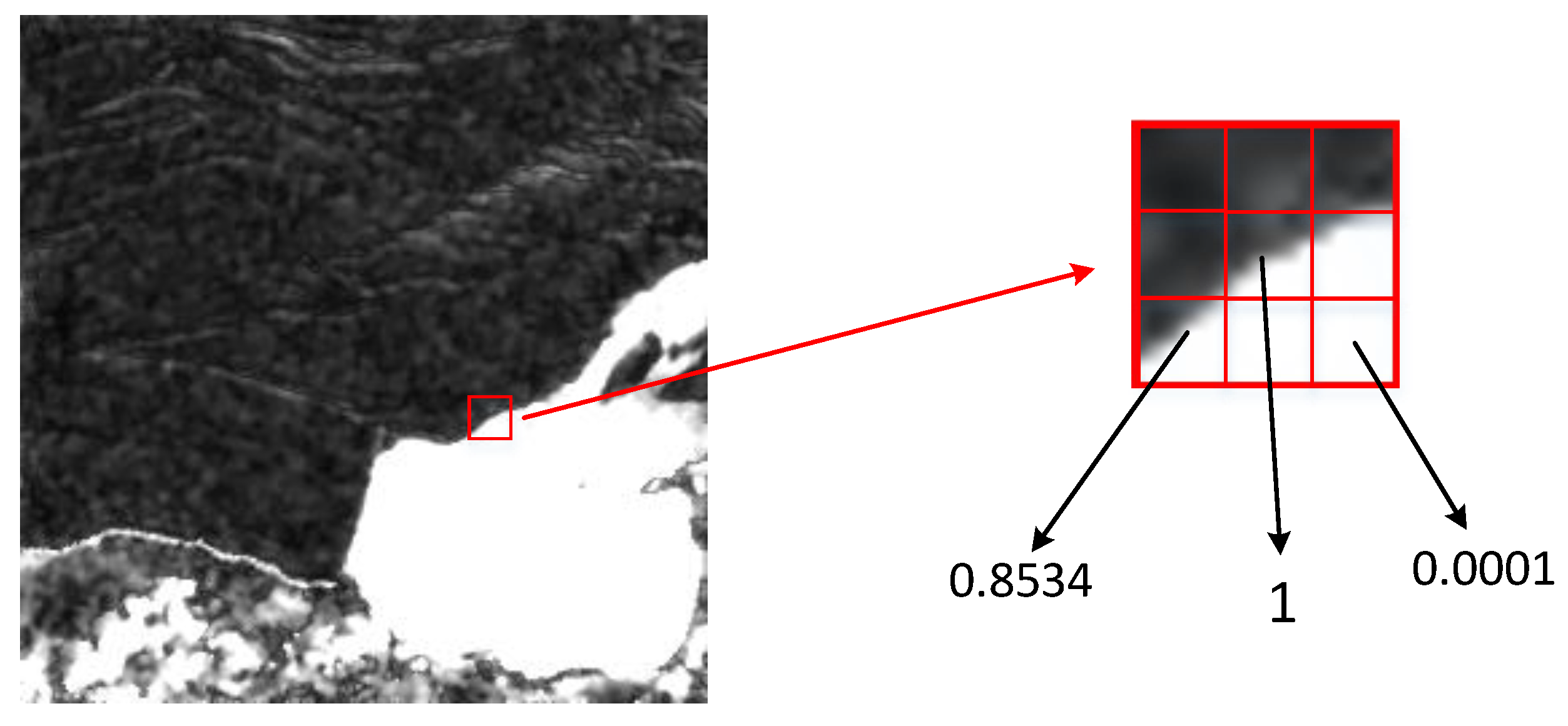
Although FLICM combines local spatial information and local gray-level information and has a suppressive effect on local noise, it does not consider the impact of pixel patches in different directions on the local central pixel, which may cause the loss of central pixel details in areas with severe noise. In addition, in FLICM, the introduction of the fuzzy factor ensures that the neighboring pixels have similar membership, thereby achieving a denoising effect. However, when the noise distribution is concentrated, FLICM will mistakenly include noisy pixels into the same cluster. Zhang et al. proposed an improved image clustering method that simultaneously considered self-similarity and back-projection to enhance robustness in [47], achieving a balance between noise suppression and detail preservation. Inspired by [47], considering that introducing pixel patch weights in different directions to supplement the details of the central pixel can avoid the influence of noise in the noisy area, the search window is expanded to search for pixels with local similar structures to the central pixel. The schematic diagram is shown in Figure 3, patches with different similarities are assigned different weights, and patches with similar structures are assigned higher weights, and vice versa. This can provide supplementary detail information for pixels with the same texture and edge information, and can also effectively suppress patchy noise. A pixel similarity measurement model is introduced in the search window, and adjacent pixel patches are considered with different weights.

In addition, FLICM is insufficient in considering the correlation of pixels only through spatial distance, which will further reduce the performance. Therefore, in order to effectively suppress speckle noise, we improve FLICM by expanding the search window, introducing pixel similarity measurement and spatial weighted information.

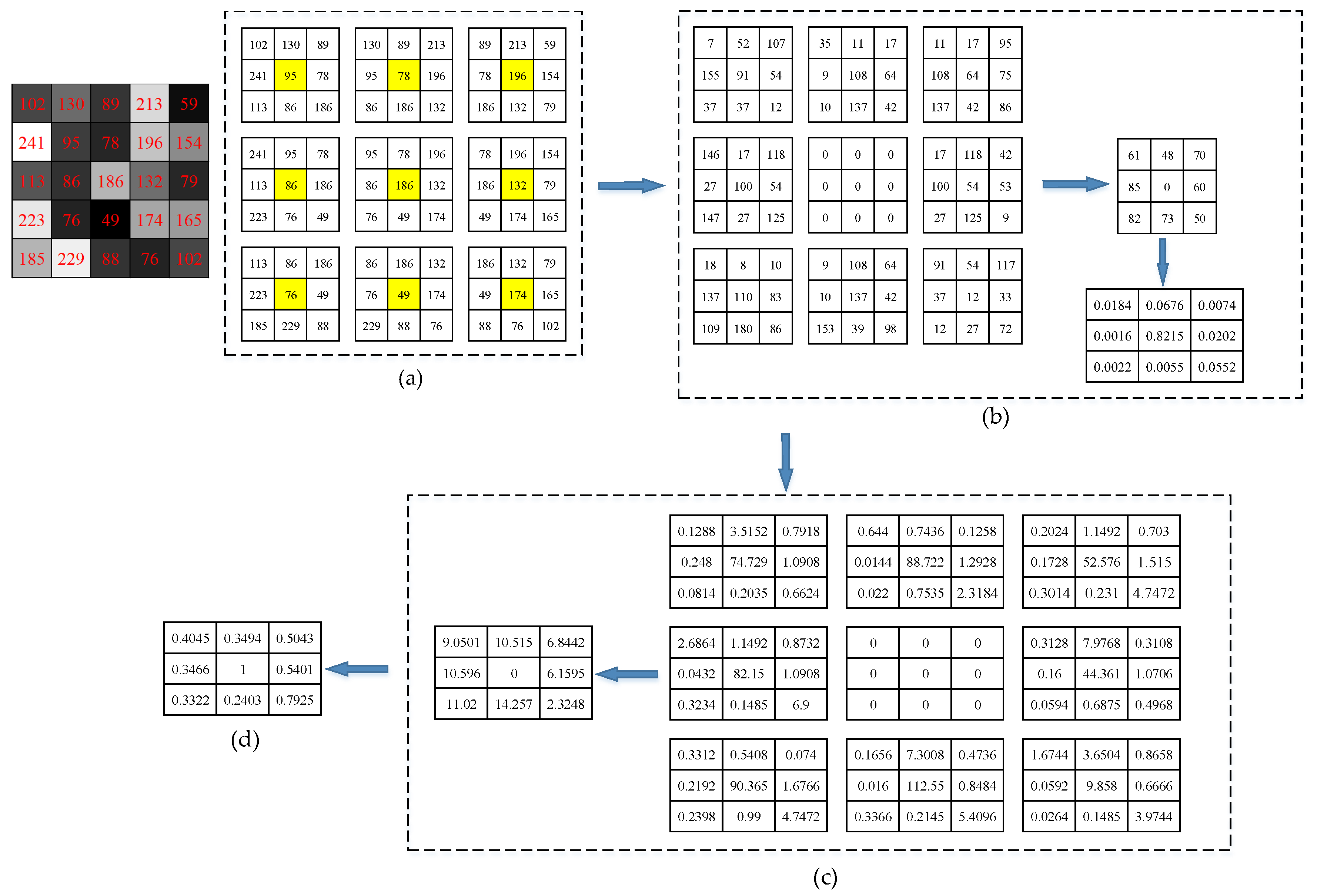
Referring to the pixel relevance model mentioned in [47], the calculation example is shown in Figure 4. For any pixel in the image, an image patch $X_i$ is constructed, and its adjacent pixel patches are $X_j$. The pixel patch size in the figure is 3 × 3, and the search window size is assumed to be 5 × 5.

The steps for calculating pixel relevance are as follows:

1. Nine image patches centered on adjacent pixels were constructed, as shown in Figure 4a;

2. Calculate the difference between the adjacent pixel patches and the central pixel patch: ${\mathit{d}}_{\mathit{i}}\left(\mathit{j}\right)$$={\displaystyle \frac{1}{\left|N_i\right|}}\sum \left|{\mathit{X}}_i-{\mathit{X}}_j\right|$, $N_i$ is the number of adjacent pixel patches, and then the weights of different directions are calculated based on the differences between the image patches: ${\mathit{w}}_{\mathit{i}}\left(\mathit{j}\right)={\displaystyle \frac{exp\left(-\alpha {\mathit{d}}_{\mathit{i}}\left(\mathit{j}\right)\right)}{{\sum }_{j\in N_i}exp\left(-\alpha {\mathit{d}}_{\mathit{i}}\left(\mathit{j}\right)\right)}}$, $\alpha$ is usually set to 0.1 to prevent the result from being too small. The whole process is shown in Figure 4b;

3. According to the image patch differences and different direction weights obtained in step 2, calculate the weighted distances in different directions: ${\mathit{d}}_{\mathit{i}}^{\mathit{w}}\left(\mathit{p}\right)={\displaystyle \frac{1}{\left|N_i\right|}}{\sum }_i\left({\mathit{w}}_{\mathit{i}}\odot \left|{\mathit{X}}_{\mathit{i}}-{\mathit{X}}_{\mathit{p}}\right|\right)$, where ⊙ represents the dot product of two vector matrices, as shown in Figure 4c;

4. Calculate the correlation between adjacent pixels and the central pixel: $\mathit{s}(\mathit{i},\mathit{j})$$=exp\left(-\alpha {\mathit{d}}_{\mathit{i}}^{\mathit{w}}\left(\mathit{j}\right)\right)$, as shown in Figure 4d.

We modify the fuzzy factor $G_{ki}$, add the local patch pixel correlation and spatial information weight, and generate a new factor $G_{ki}^{\prime }$ as follows:

$$G_{ki}^{\prime }=\sum _{j\in N_i;i\ne j}s(i,j){\left(1-u_{kj}\right)}^m{∥\sum _{p\in W_j^r}{w}_{jp}{x}_p-v_k∥}^2,$$

(15)

where $W_j^r$ represents the set of neighborhood pixels centered on pixel j, r represents the side length of the neighborhood window, and the window size is set to 5 × 5. The spatial local information is introduced to weight the pixels so that all pixels in the window can be reconstructed by their neighboring pixels, which plays a good role in suppressing isolated speckle noise and makes the algorithm more robust to noise. $w_{jp}$ represents the weight coefficient. If the pixel center is closer to its neighboring pixels, the weight will be larger, and vice versa. $w_{jp}$ is calculated by Euclidean distance, $w_{jp}={\displaystyle \frac{1}{d_{jp}}}/{\sum }_{j\in N_i}{\displaystyle \frac{1}{d_{jp}}}$, and ${\sum }_{p\in N_j}{w}_{jp}=1$. The improved fuzzy factor $G_{ki}^{\prime }$ reflects the similarity between the neighborhood pixel patches in different directions and the central pixel, supplements the structural information of the changing area, at the same time, pixel reconstruction suppresses speckle noise.

The improved algorithm clustering objective function is

$$J_m^{\prime }=\sum _{i=1k=1}^N\sum _{ki}^c\left[u_{ki}^m{∥x_i-v_k∥}^2+{G_{ki}}^{\prime }\right].$$

(16)

The updated cluster center and membership matrix formulas are as follows:

$$v_k^{\prime }={\displaystyle \frac{{\sum }_{i=1}^N{u}_{ki}^m{x}_i}{{\sum }_{i=1}^N{u}_{ki}^m}},$$

(17)

$$u_{ki}^{\prime }={\displaystyle \frac{1}{{\sum }_{j=1}^c{\left(\frac{{∥x_i-v_k∥}^2+{G_{ki}}^{\prime }}{{∥x_i-x_j∥}^2+{G_{ki}}^{\prime }}\right)}^{\frac{1}{m-1}}}}.$$

(18)

Therefore, in the objective function of the algorithm in this paper, the local patch similarity information extended near the pixel is further used to classify the close elements into one category. At the same time, the spatial information weighting is used to increase the noise resistance and improve the clustering performance. The improved clustering algorithm of this paper is called Fuzzy Local Patch Similarity Information C-Means (FLPSICM). The steps of FLPSICM are shown in Algorithm 1.

Algorithm 1: Procedure of FLPSICM
Step 1	Set the number c of cluster centers, hyperparameters m and the stopping condition $\mathcal{E}$.
Step 2	Randomly initialize the membership matrix.
Step 3	Set the loop count, starting from 0.
Step 4	Update the cluster center ${\mathit{v}}_{\mathit{k}}$ by Formula (17).
Step 5	Update the membership matrix $u_{ki}^{\prime }$ through Formula (18).
Step 6	Stop if the distance between cluster centers is less than $\mathcal{E}$ or the maximum number of iterations is reached, otherwise repeat steps 4 and 5.
Step 7	Assign the pixel to the class with the highest membership by ${\mathit{C}}_{\mathit{i}}={arg}_k\left\{max\left\{{\mathit{u}}_{\mathit{ki}}\right\}\right\},k=1,2,\dots ,c.$

3. Experiments and Analysis

This section discusses the impact of different difference images and different clustering analysis methods on the result indicators. After comprehensive comparison, the difference image and clustering analysis methods have the best indicators. Section 3.1 introduces the dataset and evaluation criteria. Section 3.2–Section 3.4 are ablation experiments, and Section 3.5 and Section 3.6 are the comparison of change detection results with the latest methods and experimental results on a large scale dataset.

3.1. Datasets and Evaluation Criteria

There are four experimental datasets used in the experiments, including Yellow River farmland, San Francisco, Sulzberg, and Inland waters. Figure 5, Figure 6, Figure 7 and Figure 8 show the visualization of the four datasets, which have been geometrically corrected and registered, and the real change images have been manually calibrated, where (a) and (b) are satellite images at different times, (c) is the manually calibrated reference image. The information of the four datasets is detailed in

Table 1. Source information of the 4 experimental datasets.

Place	Pre-Time	Post-Time	Size	Satellite	Resolution
Farmland	2008.06	2009.06	306 × 291	Radarsat-2	8 m
San Francisco	2003.08	2004.05	256 × 256	ERS-2	20 m
Sulzberger	2011.03.11	2011.03.16	256 × 256	Envisat	10 m
Inland river	2008.06	2009.06	291 × 444	Radarsat-2	8 m

.

Evaluation metrics include false positive (FP), false negative (FN), overall error (OE), percentage of correct classification (PCC) and Kappa coefficient (KC). FP represents the number of unchanged pixels detected as changed pixels, and FN represents the number of changed pixels misclassified as unchanged pixels. OE represents the sum of FP and FN. PCC represents the percentage of correctly classified pixels in the total pixels. PCC is defined as follows:

$$PCC={\displaystyle \frac{TP+TN}{TP+FP+TN+FN}},$$

(19)

where TP and TN are true positives and true negatives, representing correctly classified changed pixels and correctly classified unchanged pixels, respectively.

KC is a comprehensive indicator, defined as follows:

$$KC={\displaystyle \frac{PCC-PRE}{1-PRE}},$$

(20)

$$PRE={\displaystyle \frac{(TP+FN)\times (TP+FP)+(TN+FP)\times (TN+FN)}{{(TP+FP+TN+FN)}^2}}.$$

(21)

3.2. Difference Image Generation Comparison

Generally speaking, difference image generation is crucial for difference image analysis because it contains many potential change areas. To analyze the effectiveness of the curvelet fusion difference image, we added additional experiments to compare the final change images and metrics produced by different difference images, and clustering method for subsequent analysis remained unchanged.

We compare curvelet fusion difference image with the difference images of LR operator, RMR operator, neighborhood ratio operator and wavelet-based fusion method. The difference images obtained using different methods on the four datasets are shown in Figure 9, Figure 10, Figure 11 and Figure 12.

For the first dataset, the Yellow River farmland, and the second dataset, San Francisco, it can be clearly seen from Figure 9 and Figure 10 that the LR operator retains the background information very well, but at the same time there is a lot of noise. The RMR operator plays a denoising role, but the change area is suppressed. The neighborhood-based ratio difference image presents a lower gray value, which has a good effect on preserving unchanged areas. At the same time, it also weakens the representation of changed areas and makes the representation of edge details vague. Wavelet fusion difference image produces a relatively smooth effect, which effectively reflects the changed and unchanged areas, but the representation of edges and changed areas is not as good as curvelet fusion difference image. Curvelet fusion can effectively combine the advantages and disadvantages of the two algorithms, retaining the background information, suppressing the noise, and highlighting the changed areas. For the third data set, Figure 11 also shows visually that the LR operator retains more overall information, the RMR operator has a more obvious effect in suppressing noise, the curvelet fusion image combines the advantages of two difference images. The neighborhood-based ratio difference image and the wavelet transform-based fusion difference image have good information representation of the unchanged area, but the representation of the changed area is not perfect. The gray value of the changed area is low, and the wavelet fusion image has poor representation of edges and line segments. For the inland waters of the fourth dataset, as shown in Figure 12, the neighborhood-based ratio difference image has a poor representation of edge details, and the wavelet fusion image has a poor representation in the changed area. The fusion image based on curvelet transform enhances the representation of changed and unchanged areas by modifying the frequency domain coefficients of the LR operator image and the RMR operator image. It effectively combines the frequency information of the two operator images and the multi-scale advantages of curvelet, and uses anisotropy to effectively retain the curve information in the edges and textures, thus fully representing the changed areas.

The Kappa coefficients and PCCs of different difference images in each scene after image segmentation by FLPSICM are compared, and the resulting line charts are shown in Figure 13 and Figure 14. It can be seen from the line chart that the final Kappa coefficients and PCCs of the difference image selection curvelet fusion image in the four scenes are all optimal. This also proves that the curvelet fusion image combines the useful complementary information of different difference images.

3.3. Comparison of Curvelet Fusion Scale Levels

In the curvelet fusion difference image, the decomposition scale number has a significant impact on the fusion result. In general, the higher the scale, the richer the image texture representation, but at the same time there will be more noise and greater computational complexity. So we choose different scale levels to show the impact on the results. Figure 15 shows the PCC of each dataset at different scales, and Figure 16 shows the running time of each dataset at different scales. We set the decomposition scale to 3, 4, 5, 6, and 7 respectively. As can be seen from Figure 16, the broken line shows a linear trend. The larger the scale, the longer the running time. As can be seen from Figure 15, in almost every data set, the PCC is highest when the decomposition scale is 5. In summary, we set the scale level of all other experiments to 5.

3.4. Comparison of Clustering Methods

For the curvelet fusion difference image, we analyze the impact of different clustering methods for the final results. The proposed FLPSICM is used together with FCM [25], FGFCM [48], and FLICM [26] for visual and quantitative analysis. The Farmland dataset and San Francisco dataset are used as examples for visual and quantitative analysis. The final result display and indicators are presented in Figure 17 and Figure 18 and

Table 2. Performance indicators for Farmland dataset in different cluster methods.

Cluster	FP	FN	OE	PCC (%)
FCM	1851	497	2348	97.36
FGFCM	632	685	1317	98.52
FLICM	256	809	1065	98.80
FLPSICM	197	696	893	99.00

and

Table 3. Performance indicators for San Francisco dataset in different cluster methods.

Cluster	FP	FN	OE	PCC (%)
FCM	702	371	1073	98.36
FGFCM	515	479	994	98.48
FLICM	377	478	855	98.70
FLPSICM	312	365	677	98.98

.

As can be seen from Figure 17 and Figure 18, for the farmland scene and San Francisco scene, since FCM ignores context information, it leads to a lot of noise, so FP number is also the most. FLPSICM has better noise suppression than FCM. Since it combines the local space and gray-level neighborhood to form a nonlinear weighted image, it directly clusters the gray histogram and has a very short calculation time. FLICM combines local spatial information and local gray-level information. Compared with FGFCM, it directly uses the original image and introduces a new fuzzy factor to improve noise robustness. Visually, it can be seen that FLICM has significantly improved noise robustness compared with FCM and FGFCM, but it also loses some details, resulting in more FNs, and the retention of image edge details is not as good as FLPSICM. FLPSICM achieves a very good results in preserving image details and suppressing noise.

In addition, we added experiments of different noise types and different noise intensities on the two original SAR images. We added Gaussian noise and speckle noise of different intensities to the Yellow River farmland, and selected PSNR and SSIM as evaluation indicators. The results are shown in Figure 19 and

Table 4. Denoising evaluation indicators after adding different noises.

Noise Type	PSNR/dB	SSIM
0	21.36	0.9502
Gaussian noise 0.1	20.95	0.9477
Gaussian noise 0.2	20.47	0.9446
Speckle noise 0.4	20.19	0.9396
Speckle noise 0.8	19.48	0.9308

.

As can be seen from Figure 19 and Table 4, the PSNR and SSIM of our method is high in different noise environments, and as the noise intensity increases, the index decreases slightly. From the visualization results, there is no severe noise. This proves that our method is robust to noise.

3.5. Comparison and Analysis of Change Detection Experiment Results

In this section, the visual and quantitative results of our method for SAR image detection are compared with eight existed popular methods, including FCM [49], RFLICM [27], CWNN [32], NR-ELM [50], GaborPCANet [31], DDNet [51], ShearNet [42], and LANTNet [52]. The resulting image is finally presented as a binary image, with white representing the changed area and black representing the unchanged area. The visualization results on four datasets shown in Figure 20, Figure 21, Figure 22 and Figure 23. The performance indicators are shown in

Table 5. Performance indicators for Farmland dataset in different methods.

Method	FP	FN	OE	PCC (%)	KC (%)
FCM [49]	2472	880	3352	96.23	70.39
RFLICM [27]	1381	467	1848	97.92	82.76
NR-ELM [50]	165	1480	1645	98.15	83.43
PCANet [31]	25	1312	1337	98.50	84.77
CWNN [32]	324	734	1058	98.81	88.93
DDNet [51]	260	847	1107	98.76	88.22
ShearNet [42]	211	752	963	98.92	89.80
LANTNet [52]	1392	632	2024	97.73	80.88
CF-LPSICM	197	696	893	99.00	90.57

,

Table 6. Performance indicators for San Francisco dataset in different methods.

Method	FP	FN	OE	PCC (%)	KC (%)
FCM [49]	1783	408	2191	96.65	77.82
RFLICM [27]	884	442	1326	98.03	85.78
NR-ELM [50]	422	457	879	98.66	89.86
PCANet [31]	141	646	787	98.79	90.48
CWNN [32]	437	295	732	98.88	91.70
DDNet [51]	1003	280	1283	98.04	86.23
ShearNet [42]	445	395	840	98.71	90.39
LANTNet [52]	1777	275	2052	96.87	79.45
CF-LPSICM	312	365	677	98.98	92.18

,

Table 7. Performance indicators for Sulzberger dataset in different methods.

Method	FP	FN	OE	PCC (%)	KC (%)
FCM [49]	1379	621	2000	96.95	90.40
RFLICM [27]	593	356	949	98.55	95.37
NR-ELM [50]	65	1435	1500	97.71	92.32
PCANet [31]	333	533	866	98.68	95.72
CWNN [32]	750	257	1007	98.46	95.13
DDNet [51]	1379	109	1488	97.73	92.96
ShearNet [42]	463	220	683	98.95	96.67
LANTNet [52]	157	971	1128	98.28	94.32
CF-LPSICM	297	260	557	99.15	97.27

and

Table 8. Performance indicators for Inland river dataset in different methods.

Method	FP	FN	OE	PCC (%)	KC (%)
FCM [49]	3268	543	3811	97.05	64.63
RFLICM [27]	1654	798	2452	98.10	72.84
NR-ELM [50]	735	1186	1921	98.51	75.40
PCANet [31]	622	1770	2392	98.15	71.01
CWNN [32]	1559	482	2041	98.42	77.90
DDNet [51]	1513	526	2039	98.42	77.72
ShearNet [42]	727	1115	1842	98.57	76.58
LANTNet [52]	2215	376	2591	97.99	73.95
CF-LPSICM	845	877	1722	98.67	79.01

.

For the Yellow River farmland dataset, it can be seen from Table 5 that the PCC and KC of our method are 99.00% and 90.57%, which are the best compared with other methods. Since FCM are sensitive to noise, the FP index is highest. However, RFLICM introduces a local similarity metric to supplement the local pixel information, so the FN index is the lowest. In NR-ELM and PCANet, more uncertain pixels are provided in the pre-classification, and it is difficult to provide enough samples, resulting in many pixels not being detected, so the FN index is relatively high. Thanks to the fact that PCANet is very robust in suppressing speckle noise, as can be seen from Figure 20d, the number of false alarm pixels is minimal, only 25. CWNN addresses the problem of insufficient training samples, so its FPs and FNs are relatively low. DDNet is similar to CWNN, achieving a balance between FP and FN. The OE of ShearNet is second only to the CF-LPSICM, and has only 70 errors more than the proposed method. Visually, it can be seen that the FP and FN of the image are well maintained, thanks to the excellent hierarchical representation of shearlet and curvelet in the frequency domain. As shown in Figure 20h, LANTNet has a large number of FPs but maintains a good FN. Our method has a good effect on false alarm suppression from a visual perspective, but the contour representation of the changing area in the lower right corner is not perfect, resulting in slightly more FN, but the overall comprehensive performance is optimal.

For the San Francisco dataset, from the visualization results, we can see that FCM has a lot of noise and the FP index is the highest. RFLICM introduces a new fuzzy factor to suppress noise, so the background noise suppression is better than FCM. PCANet is a classification model with strong noise robustness, so it suppresses noise very well and has the least FP number, just 141. However, there are fewer reliable samples in the pre-classification, resulting in a large number of FNs. From the red circle in Figure 21d, we can see that many change areas are not detected. LANTNet has a large number of false alarm pixels, but the number of missed detection pixels is the least, only 275. CWNN has good control over both missed alarms and false alarms, but the representation of the changing area in the upper left corner is not sufficient. From Figure 21i and the index results, we can see that CF-LPSICM has achieved good results in controlling both false alarms and missed alarms, so OE is least. Most importantly, The PCC and KC of CF-LPSICM reached 98.98% and 92.18%, which is the best compared with other methods.

For the Sulzberger dataset, it can be clearly seen visually that FCM has the most serious noise. NR-ELM and LANTNet have poor representation of the changing area in the lower left corner of the image as shown in the red circles in Figure 22c,h, with a large number of FNs. NR-ELM has many missed detection areas in the large changing area in the lower right corner. However, NR-ELM has the least FP number, just 65, thanks to the NR operator in NR-ELM. DDNet has the least number of missed pixels, only 109, but at the same time the number of FP is most, as can be clearly seen from the red box in Figure 22f. It is worth noting that both ShearNet and CF-LPSICM have low FP and FN numbers, but the OE number of CF-LPSICM is 126 lower than that of ShearNet. The proposed method CF-LPSICM has good control over FP and FN. Benefiting from the hierarchical expression of curvelet decomposition, it represents the contour of the changing area and has an obvious noise suppression effect. In terms of evaluation criteria, the KC value of the proposed CF-LPSICM is improved by 6.87%, 1.9%, 4.95%, 1.55%, 2.14%, 4.31%, 0.6%, and 2.95% over FCM, RFLICM, NR-ELM, PCANet, CWNN, DDNet, ShearNet, and LANTNet, respectively. Visually and metrically, the proposed method achieved a balance between FP and FN.

The visualization results and performance indicators for inland waters are shown in Figure 23 and Table 8, respectively. FCM, RFLICM, CWNN, DDNet, and LANTNet all have the situation of high FP, while NR-ELM, PCANet, and ShearNet have the problem of high FN. CWNN and DDNet have the same characteristics, high FP and low FN, due to the influence of network performance. PCANet has the lowest FP, thanks to the combination of PCANet and traditional methods to improve accuracy, but at the same time, it has the highest FN. LANTNet has the least FN but a high FP. These two methods also illustrate the instability of network performance. The CF-LPSICM achieves a good performance in controlling both FP and FN, suppressing noise as much as possible while retaining image details, so OE are the best indicators. ShearNet has the same advantages as CF-LPSICM, but the PCC value of CF-LPSICM is 0.1% higher than that of ShearNet, and the KC value is 2.43% higher. The CF-LPSICM achieves the best PCC and KC values. CF-LPSICM is better in preserving details in the changing area.

3.6. Experimental Results on a Large-Scale Dataset

We conducted experiments on a large dataset. The experimental dataset is Elephant Butte, with a size of 1200 × 2400, taken in August 1991 and August 2011.

As can be seen from Figure 24, our method has good denoising performance on large-scale images, and there is no background noise. As can be seen from

Table 9. Performance indicators for Elephant Butte dataset in different methods.

Method	FP	FN	OE	PCC (%)	KC (%)
PCA-K	57,245	12,433	69,678	97.58	76.60
DDNet	34,127	24,609	58,736	97.96	77.90
CF-LPSICM	33,792	2729	36,521	98.73	87.43

, the PCC and KC of the proposed method are the highest. Visualization and indicators prove that the proposed method is still robust in large-scale scenes.

4. Conclusions

In this paper, we propose a novel unsupervised SAR image change detection method based on curvelet fusion and local patch similarity clustering, referred to as CF-LPSICM. Experiments show that curvelet fusion can make full use of the complementary information of different difference images, and the fused image contains a complete potential change area. For difference image analysis, a novel clustering algorithm combining local patch similarity information and local spatial weighting is proposed. Experiments show that the algorithm is robust to noise, while denoising, it also retains the details and improves the adaptability of the algorithm. The average values of PCC and KC reached 98.95% and 89.76%, which are the best among the latest methods. However, the computational complexity of curvelet decomposition increases with the size of the processed image, which will lead to a decrease in detection performance. In addition, considering the combination of unsupervised methods and deep learning, we can overcome the dependence of traditional neural networks on labeled samples and develop new semi-supervised methods.

References

1. Reigber, A.; Scheiber, R.; Jager, M.; Prats-Iraola, P.; Hajnsek, I.; Jagdhuber, T.; Papathanassiou, K.P.; Nannini, M.; Aguilera, E.; Baumgartner, S.; et al. Very-high-resolution airborne synthetic aperture radar imaging: Signal processing and applications. Proc. IEEE 2012, 101, 759–783. [Google Scholar] [CrossRef]
2. Oliver, C.; Quegan, S. Understanding Synthetic Aperture Radar Images; SciTech Publishing Inc.: Raleigh, NC, USA, 2004. [Google Scholar]
3. Rao, A.; Jung, J.; Silva, V.; Molinario, G.; Yun, S.H. Earthquake building damage detection based on synthetic-aperture-radar imagery and machine learning. Nat. Hazards Earth Syst. Sci. 2023, 23, 789–807. [Google Scholar] [CrossRef]
4. Semenzato, A.; Pappalardo, S.E.; Codato, D.; Trivelloni, U.; De Zorzi, S.; Ferrari, S.; De Marchi, M.; Massironi, M. Mapping and monitoring urban environment through sentinel-1 SAR data: A case study in the Veneto region (Italy). ISPRS Int. J. Geo-Inf. 2020, 9, 375. [Google Scholar] [CrossRef]
5. Chen, J.; Xiong, R.; Yu, H.; Xu, G.; Xing, M. Nonparametric Full-Aperture Autofocus Imaging for Microwave Photonic SAR. IEEE Trans. Geosci. Remote Sens. 2024, 62, 5214815. [Google Scholar] [CrossRef]
6. Chen, J.; Li, M.; Yu, H.; Xing, M. Full-Aperture Processing of Airborne Microwave Photonic SAR Raw Data. IEEE Trans. Geosci. Remote Sens. 2023, 61, 5218812. [Google Scholar] [CrossRef]
7. Yahya, N.; Kamel, N.S.; Malik, A.S. Subspace-based technique for speckle noise reduction in SAR images. IEEE Trans. Geosci. Remote Sens. 2014, 52, 6257–6271. [Google Scholar] [CrossRef]
8. Qiu, F.; Berglund, J.; Jensen, J.R.; Thakkar, P.; Ren, D. Speckle noise reduction in SAR imagery using a local adaptive median filter. GISci. Remote Sens. 2004, 41, 244–266. [Google Scholar] [CrossRef]
9. Mansourpour, M.; Rajabi, M.; Blais, J. Effects and performance of speckle noise reduction filters on active radar and SAR images. Proc. ISPRS 2006, 36, W41. [Google Scholar]
10. Choi, H.; Jeong, J. Speckle noise reduction technique for SAR images using statistical characteristics of speckle noise and discrete wavelet transform. Remote Sens. 2019, 11, 1184. [Google Scholar] [CrossRef]
11. Sansosti, E.; Berardino, P.; Manunta, M.; Serafino, F.; Fornaro, G. Geometrical SAR image registration. IEEE Trans. Geosci. Remote Sens. 2006, 44, 2861–2870. [Google Scholar] [CrossRef]
12. Alatalo, J.; Sipola, T.; Rantonen, M. Improved Difference Images for Change Detection Classifiers in SAR Imagery Using Deep Learning. IEEE Trans. Geosci. Remote Sens. 2023, 61, 5218714. [Google Scholar] [CrossRef]
13. Wang, R.; Chen, J.W.; Wang, Y.; Jiao, L.; Wang, M. SAR Image Change Detection via Spatial Metric Learning With an Improved Mahalanobis Distance. IEEE Geosci. Remote Sens. Lett. 2020, 17, 77–81. [Google Scholar] [CrossRef]
14. Li, W.; Xiao, X.; Xiao, P.; Wang, H.; Xu, F. Change Detection in Multitemporal SAR Images Based on Slow Feature Analysis Combined With Improving Image Fusion Strategy. IEEE J. Sel. Top. Appl. Earth Obs. Remote Sens. 2022, 15, 3008–3023. [Google Scholar] [CrossRef]
15. Bovolo, F.; Bruzzone, L. A detail-preserving scale-driven approach to change detection in multitemporal SAR images. IEEE Trans. Geosci. Remote Sens. 2005, 43, 2963–2972. [Google Scholar] [CrossRef]
16. Inglada, J.; Mercier, G. A new statistical similarity measure for change detection in multitemporal SAR images and its extension to multiscale change analysis. IEEE Trans. Geosci. Remote Sens. 2007, 45, 1432–1445. [Google Scholar] [CrossRef]
17. Gong, M.; Cao, Y.; Wu, Q. A neighborhood-based ratio approach for change detection in SAR images. IEEE Geosci. Remote Sens. Lett. 2011, 9, 307–311. [Google Scholar] [CrossRef]
18. Zheng, Y.; Zhang, X.; Hou, B.; Liu, G. Using combined difference image and k-means clustering for SAR image change detection. IEEE Geosci. Remote Sens. Lett. 2013, 11, 691–695. [Google Scholar] [CrossRef]
19. Peng, Y.; Cui, B.; Yin, H.; Zhang, Y.; Du, P. Automatic SAR change detection based on visual saliency and multi-hierarchical fuzzy clustering. IEEE J. Sel. Top. Appl. Earth Obs. Remote Sens. 2022, 15, 7755–7769. [Google Scholar] [CrossRef]
20. Hou, B.; Wei, Q.; Zheng, Y.; Wang, S. Unsupervised change detection in SAR image based on gauss-log ratio image fusion and compressed projection. IEEE J. Sel. Top. Appl. Earth Obs. Remote Sens. 2014, 7, 3297–3317. [Google Scholar] [CrossRef]
21. Ma, J.; Gong, M.; Zhou, Z. Wavelet fusion on ratio images for change detection in SAR images. IEEE Geosci. Remote Sens. Lett. 2012, 9, 1122–1126. [Google Scholar] [CrossRef]
22. Zhang, W.; Jiao, L.; Liu, F.; Yang, S.; Liu, J. Adaptive contourlet fusion clustering for SAR image change detection. IEEE Trans. Image Process. 2022, 31, 2295–2308. [Google Scholar] [CrossRef] [PubMed]
23. Moser, G.; Serpico, S.B. Generalized minimum-error thresholding for unsupervised change detection from SAR amplitude imagery. IEEE Trans. Geosci. Remote Sens. 2006, 44, 2972–2982. [Google Scholar] [CrossRef]
24. Yang, G.; Li, H.C.; Yang, W.; Fu, K.; Celik, T.; Emery, W.J. Variational Bayesian change detection of remote sensing images based on spatially variant Gaussian mixture model and separability criterion. IEEE J. Sel. Top. Appl. Earth Obs. Remote Sens. 2019, 12, 849–861. [Google Scholar] [CrossRef]
25. Bezdek, J.C.; Ehrlich, R.; Full, W. FCM: The fuzzy c-means clustering algorithm. Comput. Geosci. 1984, 10, 191–203. [Google Scholar] [CrossRef]
26. Krinidis, S.; Chatzis, V. A robust fuzzy local information C-means clustering algorithm. IEEE Trans. Image Process. 2010, 19, 1328–1337. [Google Scholar] [CrossRef]
27. Gong, M.; Zhou, Z.; Ma, J. Change detection in synthetic aperture radar images based on image fusion and fuzzy clustering. IEEE Trans. Image Process. 2011, 21, 2141–2151. [Google Scholar] [CrossRef]
28. Mu, C.; Huo, L.; Liu, Y.; Liu, R.; Jiao, L. Change Detection for Remote Sensing Images Based on Wavelet Fusion and PCA-Kernel Fuzzy Clustering. Acta Electron. Sin. 2015, 43, 1375–1381. [Google Scholar]
29. Yan, W.; Shi, S.; Pan, L.; Zhang, G.; Wang, L. Unsupervised change detection in SAR images based on frequency difference and a modified fuzzy c-means clustering. Int. J. Remote Sens. 2018, 39, 3055–3075. [Google Scholar] [CrossRef]
30. Cui, B.; Peng, Y.; Zhang, Y.; Yin, H.; Fang, H.; Guo, S.; Du, P. Enhanced Edge Information and Prototype Constrained Clustering for SAR Change Detection. IEEE Trans. Geosci. Remote Sens. 2024, 62, 5206116. [Google Scholar] [CrossRef]
31. Gao, F.; Dong, J.; Li, B.; Xu, Q. Automatic change detection in synthetic aperture radar images based on PCANet. IEEE Geosci. Remote Sens. Lett. 2016, 13, 1792–1796. [Google Scholar] [CrossRef]
32. Gao, F.; Wang, X.; Gao, Y.; Dong, J.; Wang, S. Sea ice change detection in SAR images based on convolutional-wavelet neural networks. IEEE Geosci. Remote Sens. Lett. 2019, 16, 1240–1244. [Google Scholar] [CrossRef]
33. Zhang, K.; Lv, X.; Guo, B.; Chai, H. Unsupervised SAR Image Change Detection Based on Histogram Fitting Error Minimization and Convolutional Neural Network. Remote Sens. 2023, 15, 470. [Google Scholar] [CrossRef]
34. Zhang, X.; Cheng, S.; Wang, L.; Li, H. Asymmetric cross-attention hierarchical network based on CNN and transformer for bitemporal remote sensing images change detection. IEEE Trans. Geosci. Remote Sens. 2023, 61, 2000415. [Google Scholar] [CrossRef]
35. Chen, G.; Zhao, Y.; Mouthaan, K. Joint Spatial-frequency Scattering Network for Unsupervised SAR Image Change Detection. IEEE Geosci. Remote Sens. Lett. 2025, 22, 4004505. [Google Scholar] [CrossRef]
36. Dong, H.; Du, X.; Li, Z.; Li, X.; Ma, Z.F.; Gao, F.; Jiao, L. Dynamic Bilinear Fusion Network for Synthetic Aperture Radar Image Change Detection. IEEE Geosci. Remote Sens. Lett. 2025, 22, 4004005. [Google Scholar] [CrossRef]
37. Xie, J.; Gao, F.; Zhou, X.; Dong, J. Wavelet-Based Bi-Dimensional Aggregation Network for SAR Image Change Detection. IEEE Geosci. Remote Sens. Lett. 2024, 21, 4013705. [Google Scholar] [CrossRef]
38. Samek, W.; Montavon, G.; Lapuschkin, S.; Anders, C.J.; Müller, K.R. Explaining deep neural networks and beyond: A review of methods and applications. Proc. IEEE 2021, 109, 247–278. [Google Scholar] [CrossRef]
39. Traore, B.B.; Kamsu-Foguem, B.; Tangara, F. Deep convolution neural network for image recognition. Ecol. Inform. 2018, 48, 257–268. [Google Scholar] [CrossRef]
40. Gong, M.; Zhao, J.; Liu, J.; Miao, Q.; Jiao, L. Change detection in synthetic aperture radar images based on deep neural networks. IEEE Trans. Neural Netw. Learn. Syst. 2015, 27, 125–138. [Google Scholar] [CrossRef]
41. Zhao, G.; Peng, Y. Semisupervised SAR image change detection based on a siamese variational autoencoder. Inf. Process. Manag. 2022, 59, 102726. [Google Scholar] [CrossRef]
42. Dong, H.; Jiao, L.; Ma, W.; Liu, F.; Liu, X.; Li, L.; Yang, S. Deep Shearlet Network for Change Detection in SAR Images. IEEE Trans. Geosci. Remote Sens. 2022, 60, 5241115. [Google Scholar] [CrossRef]
43. Zhang, X.; Su, H.; Zhang, C.; Gu, X.; Tan, X.; Atkinson, P.M. Robust unsupervised small area change detection from SAR imagery using deep learning. ISPRS J. Photogramm. Remote Sens. 2021, 173, 79–94. [Google Scholar] [CrossRef]
44. Xuan, J.; Xin, Z.; Liao, G.; Huang, P.; Wang, Z.; Sun, Y. Change detection based on fusion difference image and multi-scale morphological reconstruction for SAR images. Remote Sens. 2022, 14, 3604. [Google Scholar] [CrossRef]
45. Ma, J.; Plonka, G. The curvelet transform. IEEE Signal Process. Mag. 2010, 27, 118–133. [Google Scholar] [CrossRef]
46. Candes, E.; Demanet, L.; Donoho, D.; Ying, L. Fast discrete curvelet transforms. Multiscale Model. Simul. 2006, 5, 861–899. [Google Scholar] [CrossRef]
47. Zhang, X.; Sun, Y.; Liu, H.; Hou, Z.; Zhao, F.; Zhang, C. Improved clustering algorithms for image segmentation based on non-local information and back projection. Inf. Sci. 2021, 550, 129–144. [Google Scholar] [CrossRef]
48. Cai, W.; Chen, S.; Zhang, D. Fast and robust fuzzy c-means clustering algorithms incorporating local information for image segmentation. Pattern Recognit. 2007, 40, 825–838. [Google Scholar] [CrossRef]
49. Ghosh, A.; Mishra, N.S.; Ghosh, S. Fuzzy clustering algorithms for unsupervised change detection in remote sensing images. Inf. Sci. 2011, 181, 699–715. [Google Scholar] [CrossRef]
50. Gao, F.; Dong, J.; Li, B.; Xu, Q.; Xie, C. Change detection from synthetic aperture radar images based on neighborhood-based ratio and extreme learning machine. J. Appl. Remote Sens. 2016, 10, 046019. [Google Scholar] [CrossRef]
51. Qu, X.; Gao, F.; Dong, J.; Du, Q.; Li, H.C. Change detection in synthetic aperture radar images using a dual-domain network. IEEE Geosci. Remote Sens. Lett. 2021, 19, 4013405. [Google Scholar] [CrossRef]
52. Meng, D.; Gao, F.; Dong, J.; Du, Q.; Li, H.C. Synthetic aperture radar image change detection via layer attention-based noise-tolerant network. IEEE Geosci. Remote Sens. Lett. 2022, 19, 4026505. [Google Scholar] [CrossRef]
Figure 1. Framework of CF-LPSICM method.
Remotesensing 17 00840 g001
Figure 2. Curvelet frequency domain tiled image.
Remotesensing 17 00840 g002
Figure 3. Schematic diagram of pixel correlation weight.
Remotesensing 17 00840 g003
Figure 4. Pixel correlation calculation example. (a) Neighborhood pixel patches construction. (b) Calculation of weights in different directions. (c) Calculation of weighted distances in different directions. (d) Relevance calculation.
Remotesensing 17 00840 g004
Figure 5. Farmland dataset. (2448 m × 2328 m) (a) Image captured in 2008.06; (b) image captured in 2009.06; (c) the ground truth.
Remotesensing 17 00840 g005
Figure 6. San Francisco dataset. (5120 m × 5120 m) (a) Image captured in 2003.08; (b) image captured in 2004.05; (c) the ground truth.
Remotesensing 17 00840 g006
Figure 7. Sulzberger dataset. (2560 m × 2560 m) (a) Image captured in 2011.03.11; (b) image captured in 2011.03.16; (c) the ground truth.
Remotesensing 17 00840 g007
Figure 8. Inland river dataset. (2328 m × 3552 m) (a) Image captured in 2008.06; (b) image captured in 2009.06; (c) the ground truth.
Remotesensing 17 00840 g008
Figure 9. Different difference image generation methods for farmland dataset. (a) LR; (b) RMR; (c) neighborhood-based ratio; (d) Wavelet fusion; (e) Curvelet fusion.
Remotesensing 17 00840 g009
Figure 10. Different difference image generation methods for San Francisco dataset. (a) LR; (b) RMR; (c) neighborhood-based ratio; (d) Wavelet fusion; (e) Curvelet fusion.
Remotesensing 17 00840 g010
Figure 11. Different difference image generation methods for Sulzberger dataset. (a) LR; (b) RMR; (c) neighborhood-based ratio; (d) Wavelet fusion; (e) Curvelet fusion.
Remotesensing 17 00840 g011
Figure 12. Different difference image generation methods for Inland river dataset. (a) LR; (b) RMR; (c) neighborhood-based ratio; (d) Wavelet fusion; (e) Curvelet fusion.
Remotesensing 17 00840 g012
Figure 13. Comparison of KCs of different difference images in different scenes.
Remotesensing 17 00840 g013
Figure 14. Comparison of PCCs of different difference images in different scenes.
Remotesensing 17 00840 g014
Figure 15. PCC comparison of different datasets at different scale levels.
Remotesensing 17 00840 g015
Figure 16. Comparison of running time on different datasets at different scales.
Remotesensing 17 00840 g016
Figure 17. Final visualization results of the Farmland dataset. (a) FCM; (b) FGFCM; (c) FLICM; (d) FLPSICM; (e) GT.
Remotesensing 17 00840 g017
Figure 18. Final visualization results of the San Francisco dataset. (a) FCM; (b) FGFCM; (c) FLICM; (d) FLPSICM; (e) GT.
Remotesensing 17 00840 g018
Figure 19. Visualization of detection results after adding different noises. (a) The ground truth; (b) Noise 0; (c) Gaussian noise 0.1; (d) Gaussian noise 0.2; (e) Speckle noise 0.4; (f) Speckle noise 0.8.
Remotesensing 17 00840 g019
Figure 20. Final visualization results of the Farmland dataset in different methods. (a) FCM; (b) RFLICM; (c) NR-ELM; (d) PCANet; (e) CWNN; (f) DDNet; (g) ShearNet; (h) LANTNet; (i) CF-LPSICM; (j) The ground truth.
Remotesensing 17 00840 g020
Figure 21. Final visualization results of the San Francisco dataset in different methods. (a) FCM; (b) RFLICM; (c) NR-ELM; (d) PCANet; (e) CWNN; (f) DDNet; (g) ShearNet; (h) LANTNet; (i) CF-LPSICM; (j) The ground truth.
Remotesensing 17 00840 g021
Figure 22. Final visualization results of the Sulzberger dataset in different methods. (a) FCM; (b) RFLICM; (c) NR-ELM; (d) PCANet; (e) CWNN; (f) DDNet; (g) ShearNet; (h) LANTNet; (i) CF-LPSICM; (j) The ground truth.
Remotesensing 17 00840 g022
Figure 23. Final visualization results of Inland water dataset in different methods. (a) FCM; (b) RFLICM; (c) NR-ELM; (d) PCANet; (e) CWNN; (f) DDNet; (g) ShearNet; (h) LANTNet; (i) CF-LPSICM; (j) The ground truth.
Remotesensing 17 00840 g023
Figure 24. Final visualization results of the Elephant Butte dataset in different methods. (a) Image obtained in 1991.08.20; (b) image obtained in 2011.08.27; (c) the ground truth. (d) PCA-K; (e) DDNet; (f) CF-LPSICM.
Remotesensing 17 00840 g024