Extraction of Periodic Terms in Satellite Clock Bias Based on Fourier Basis Pursuit Bandpass Filter

Abstract

Effective noise management and control of periodic fluctuations in spaceborne atomic clocks are essential for the accuracy and reliability of Global Navigation Satellite Systems. Time-varying periodic terms can impact both the performance evaluation and prediction accuracy of satellite clocks, making it crucial to mitigate these influences in the clock bias. We propose methods based on the Fourier dictionary and basis pursuit, namely the Fourier basis pursuit (FBP) spectrum and the Fourier basis pursuit bandpass filter (FBPBPF), to analyze and extract periodic terms in the satellite clock bias. The FBP method minimizes the L1-norm to improve spectral quality, while the FBPBPF reduces boundary effects and noise. Our experimental results show that the FBP spectrum has a more obvious main lobe and reduces spectral leakage compared to traditional windowed Fourier transforms. In simulation experiments, the FBPBPF achieves periodic term extraction with errors reduced by 6.81% to 26.55% compared to traditional signal processing methods, and boundary extraction errors reduced by up to 63.67%. Using the BeiDou Navigation Satellite System’s precise clock bias for verification, the FBP-based prediction method has significantly improved the prediction accuracy compared to the spectral analysis model. For 6, 12, 18, and 24 h predictions, the average root mean square error of the FBP prediction method is reduced by 15.85%, 11.04%, 6.45%, and 4.01%, respectively.

1. Introduction

Spaceborne atomic clocks, which are highly stable, play a crucial role in ensuring the reliability of the Global Navigation Satellite System (GNSS) [1,2]. However, due to the challenging environments in which these clocks operate, the atomic clock signals typically exhibit nonlinear, non-stationary characteristics, often containing trend, multi-periodic, and noise components [3,4]. The interplay among these elements within the satellite clock bias makes their precise separation and reconstruction a complex task.

Almost all spaceborne atomic clocks appear to exhibit periodic fluctuations [3,4,5]. Some studies attribute these periodic fluctuations to the residuals of imperfect orbit estimation or to the influence of periodic factors such as temperature and environment [3,4,6,7]. It is important to eliminate the effect of the periodic term in the clock bias in advance, as the periodic terms have a significant impact on key applications such as the performance evaluation of spaceborne atomic clocks, the fitting accuracy of the atomic clock noise coefficient, and the prediction of satellite clocks [2,6,7,8]. To achieve this, some tools are used to detect these periodic terms, such as Allan variance, Fourier transform (FT) and short-time Fourier transform (STFT) [4,9,10]. Several signal processing methods, such as the least squares method (LSM), digital filter, empirical mode decomposition (EMD), and wavelet transform, have been applied to extract the periodic terms from the clock bias [7,8,10,11,12,13].

The LSM is a traditional regression technique that models harmonic terms with constant amplitude and frequency by means of least-squares fitting. However, in practical scenarios, the satellite clock bias is non-stationary and there are systematic errors between the time-varying periodic terms and the model [8]. The digital filters based on the FT, such as finite impulse response (FIR) and infinite impulse response (IIR) filters, can reliably extract time-varying signals by selectively suppressing or preserving certain frequency components. However, sidelobes, noise components, and trend residuals in the clock bias may cause spectral peak shifts or introduce spurious frequency elements [14]. Narrow frequency bands may lead to incomplete extraction of periodic signals, while broader bands may introduce noise components and residual trends. In addition, the wavelet transform is particularly suited for non-stationary signals, but the selection of the optimal wavelet basis function often requires specialized knowledge and lacks standardization [15]. EMD has the problem of mode mixing [16]. Finally, all of these methods are susceptible to boundary effects, estimations at the beginning and end of a time series tend to be less accurate, with errors intensifying closer to the boundaries. Such distortions can compromise subsequent analyses.

To suppress sidelobe artifacts in spectral analysis and accurately extract periodic terms in satellite clock bias, this paper proposes the Fourier basis pursuit (FBP) spectrum and the Fourier basis pursuit bandpass filter (FBPBPF) methods. The FBP method employs L1-norm minimization to constrain the Fourier coefficients to obtain the FBP spectrum, thereby improving spectral resolution, suppressing sidelobes, and enhancing the main lobe. Further, the FBPBPF based on the FBP spectrum can substantially reduce boundary effects and maximally suppress noise interference. Studies using simulated and real data indicate that the FBP suppresses spectral leakage more effectively than standard windowed Fourier transform (WFT) approaches, such as rectangular, Hanning, and Blackman windows. The FBPBPF also shows significant improvements in accuracy over traditional signal extraction methods such as LSM, FIR, and IIR, particularly at the boundaries.

The remaining sections of this paper are organized as follows: Section 2 introduces the theoretical background of FBP. Section 3 discusses the modeling of the satellite clock bias and its prediction method. Section 4 uses simulated data to compare the differences between the FBP spectrum and the WFT and to analyze the feasibility of the FBPBPF in terms of reconstructing the periodic term while comparing its accuracy with the LSM, FIR, and IIR methods. The effectiveness of the proposed method is then verified using precise clock bias data from the BeiDou Navigation Satellite System (BDS) provided by the GNSS Research Center of Wuhan University (WHU). Section 5 concludes the paper.

2. Fundamentals of Fourier Basis Pursuit

The FT serves as a basic mathematical tool that transforms a time-domain signal into its frequency-domain representation. For a discrete time-domain signal $x[n]$, its discrete Fourier transform (DFT) and inverse discrete Fourier transform (IDFT) are given by:

$$X[k]=\sum _{n=0}^{N-1}x[n]·e^{-j{\displaystyle \frac{2\pi }{N}}kn}$$

(1)

$$x[n]={\displaystyle \frac{1}{N}}\sum _{k=0}^{N-1}X[k]·e^{j{\displaystyle \frac{2\pi }{N}}kn}$$

(2)

where $k,n=0, 1,\dots , N-1$, and $N$ is the data length. The index of $k$ corresponds to the angular frequency ${\varpi }_k$.

2.1. Windowing

Due to the finite length of time series, it is often related to spectral leakage, where energy from one frequency component “leaks” into adjacent frequencies. Window functions are thus applied in harmonic analysis to minimize the undesirable impact of spectral leakage. The windowed DFT is expressed as:

$$X_w[k]=\sum _{n=0}^{N-1}x[n]·w[n]·e^{-j{\displaystyle \frac{2\pi }{N}}kn}$$

(3)

where $X_w[k]$ is the DFT of the windowed signal, and $w[n]$ is the window function. Equation (1) employs a rectangular window for the time series $x[n]$. Hanning and Blackman windows are also used in this study. The definitions of the rectangular, Hanning and Blackman windows are provided in Equations (4), (5) and (6), respectively [17,18].

$$w_{rectangular}\left[n\right]=1$$

(4)

$$w_{Hanning}\left[n\right]=0.5-0.5\mathit{cos}\left({\displaystyle \frac{2\pi n}{N-1}}\right)$$

(5)

$$w_{Blackman}\left[n\right]=0.42-0.5\mathit{cos}\left({\displaystyle \frac{2\pi n}{N-1}}\right)+0.08\mathit{cos}\left({\displaystyle \frac{4\pi n}{N-1}}\right)$$

(6)

where $n=0, 1,\dots , N-1$, and $N$ is the length of the time series to be analyzed.

Employing a narrow main-lobe window function, such as the rectangular window, yields high spectral resolution, thereby enhancing the ability to distinguish closely spaced frequency components. However, the rectangular window has significant sidelobes, which may lead to substantial spectral leakage. In contrast, window functions with fast sidelobe attenuation, such as the Blackman window, significantly reduce spectral leakage, minimizing interference from sidelobes. This reduction, however, comes at the cost of some spectral resolution.

2.2. Filtering

Filtering serves the purpose of eliminating undesired components, extracting specific frequency bands, or modifying a signal’s frequency content. Filters can be implemented in various forms, such as FIR filters or IIR filters [19,20]. The output signal $y[n]$ is calculated using the convolution of the input signal $x[n]$ with the filter’s impulse response $h[n]$, as shown in Equation (7):

$$y\left[n\right]=\sum _{m=-\infty }^{+\infty }x[m]·h[n-m]$$

(7)

According to the Convolution Theorem, convolution in the time domain corresponds to multiplication in the frequency domain, as shown in Equation (8):

$$Y\left[k\right]=X[k]·H\left[k\right]$$

(8)

where $H\left[k\right]$ represents the filter’s frequency response, indicating how each frequency component will be modified. $Y\left[k\right]$ represents the filtered frequency spectrum.

The process of extracting a target signal from a mixed signal can present several challenges when it comes to filtering. IIR filters, while providing sharp transition bands, may introduce phase distortion due to their non-linear phase response. In contrast, FIR filters, despite offering a linear phase response and inherent stability, often struggle to achieve sharp transition bands and flat passbands [19,20]. For finite-length signals, boundary effects can introduce ripple or attenuation near boundaries, which can result in significant distortion at the boundary of the filtered result. Additionally, if the noise overlaps with the frequency range of the target signal, certain filters may inadvertently amplify noise components, affecting the accuracy of the filtered result.

2.3. Fourier Basis Pursuit

The sparse representation of signals has received extensive attention and research in recent years and has applications in many areas, such as signal separation, denoising, coding, tidal forecasting, and extraction of polar motion signals [21,22,23,24,25,26]. This paper applies it to the analysis and extraction of periodic terms in satellite clock bias.

Sparse representation mainly involves sparse representation algorithms and atomic dictionaries. Scholars have proposed many sparse representation algorithms, including the matching pursuit algorithm [27], the basis pursuit algorithm [28], and the frame method [29]. Scholars have proposed many atomic dictionaries to address the different characteristics of signals, such as the Fourier dictionary, warplets dictionaries [30], Chirplet dictionaries [31], etc. Mallat [32] and Chen [28] proved that the basis pursuit algorithm gives the most sparse results, and the Fourier dictionary is the simplest and most basic dictionary. Based on these two points, this paper proposes the Fourier basis pursuit spectrum and the Fourier basis pursuit bandpass filter methods.

Based on Equation (2), the matrix $\Phi$ is constructed as follows:

$$\Phi ={\left[\begin{array}{c}{e}^{j{\displaystyle \frac{2\pi }{N}}·K·0}/N\\ e^{j{\displaystyle \frac{2\pi }{N}}·K·1}/N\\ ⋮\\ e^{j{\displaystyle \frac{2\pi }{N}}·K·(N-1)}/N\end{array}\right]}_{N\times M}$$

(9)

where $K=[0, 1,\dots , M-1]$. $M$ is the number of atoms in the dictionary, and $N$ is the length of the time series. Each column of the matrix $\Phi$ represents the atom of the Fourier dictionary. The dictionary is overcomplete for $M>N$, in which case, the number of atoms is greater than the length of the time series [28]. Each atom of the Fourier dictionary demonstrates different frequency characteristics. Thus, Equation (2) can be expressed as $x=\Phi ·X$, in which $x$ is the original signal and $X$ is the corresponding coefficient vector of the Fourier dictionary.

The principle of basis pursuit is to find a representation of the signal whose coefficients have the minimum L1-norm [32]. Formally, one solves the problem if:

$$X^{*}=\underset{X\in R^p}{argmin}{‖X‖}_1 \mathit{subject} \mathit{to} \Phi ·X=x$$

(10)

The basis pursuit minimization of Equation (10) involves convex optimization that can be reformulated as a linear programming problem [32]. Through global optimization, basis pursuit can obtain a better resolution than matching pursuit and can obtain a better result than the method of frames [28,33].

The matrix $\Phi$ is the Fourier dictionary and the solution $X^{*}$ of Equation (10) is obtained according to the L1-norm. Then, the solution $X^{*}$ can be defined as the FBP spectrum. If $X^{*}$ takes the corresponding angular frequency range $[{\varpi }_1,{\varpi }_2]$, the corresponding filtering results are obtained, and the FBPBPF method can be defined as:

$$y=\Phi ·{X^{*}}_{[{\varpi }_1,{\varpi }_2]}$$

(11)

where in Equation (11), $y$ is the corresponding filtering result with angular frequency range $[{\varpi }_1,{\varpi }_2]$. Here, the difference ${\varpi }_2-{\varpi }_1$ should exceed the minimum frequency resolution, which primarily depends on the number M of atoms in the dictionary rather than the length $N$ of the time series.

This section presents a comprehensive development of the fundamental principles underpinning the FBP spectrum and the FBPBPF method, both of which are grounded in the Fourier dictionary and basis pursuit. When compared to the traditional WFT, the FBP spectrum, coupled with basis pursuit, delivers superior spectral resolution and optimal amplitude allocation at fixed frequencies. This approach effectively mitigates spectral tailing and leakage caused by finite time series lengths [34]. Furthermore, in contrast to the FIR and IIR filters typically employed in digital signal processing, the FBPBPF method, rooted in the FBP spectrum, accurately identifies and segregates coupled signals comprised of two or more quasi-periodic signals from noise, while maintaining high boundary extraction accuracy. The periodic term in the satellite clock bias is characterized as a quasi-periodic signal. In applications such as clock bias prediction and performance assessment of spaceborne atomic clocks, which often involve clock bias signals of limited length or those mixed with multiple quasi-periodic terms of similar frequencies, simulated and measured data can prove that the FBPBPF method is highly effective for extracting periodic terms.

2.4. Short-Time Fourier Transform Based on Fourier Basis Pursuit

The STFT is a common technique for analyzing non-stationary signals [8,18]. By dividing a signal into a series of short time intervals and performing an FT on each segment, the STFT enables the study of a signal’s time-frequency characteristics. The STFT is expressed as:

$$STFT\left\{x\right\}\left[m,k\right]=X_m[k]=\sum _{n=0}^{N-1}x\left[n+m\right]w\left[n\right]·e^{-j{\displaystyle \frac{2\pi }{N}}kn}\stackrel{FBP optimization}{\Rightarrow }{X}_m^{*}[k]$$

(12)

where $m$ represents the time shift of the window function, $N$ is the length of the window function, and $k$ is the frequency index. The STFT provides time-frequency localization information but has limited frequency resolution, which is constrained by the length and shape of the window function. Additionally, the STFT may exhibit sidelobe effects that can lead to spectral aliasing.

To enhance frequency resolution and suppress sidelobe effects in spectral analysis, the STFT is combined with the FBP in this study. Specifically, for the STFT result at each time shift, the Fourier coefficients are optimized according to Equation (10). The Fourier coefficients obtained through FBP optimization are then used to reconstruct the time-frequency representation, and a spectrogram is generated.

3. Satellite Clock Modeling and Prediction Methods

The BDS satellite clock bias can be modeled as a quadratic polynomial with superimposed periodic and noise terms [35], as shown in Equation (13).

$$x\left(t\right)=a+bt+{\displaystyle \frac{1}{2}}c{t}^2+\sum _{k=1}^p{A}_{k}sin(2\pi f_{k}t+{\phi }_k)+\epsilon (t)$$

(13)

where $x\left(t\right)$ represents the phase at time $t$; $a$, $b$, and $c$ are the initial phase, initial frequency offset, and frequency drift, respectively; $f_k$ is the frequency of the periodic term; ${\phi }_k$ is the initial phase of the periodic term; $\epsilon \left(t\right)$ represents the fitting error.

The spectral analysis model (SAM) is a clock prediction method based on the FT [6,7,8]. This prediction method models the clock bias using Equation (13) and extrapolates the model to obtain future clock bias values. Usually, the parameter $p$ and $f_k$ are obtained from spectral analysis, and the parameters $A_k$ and ${\phi }_k$, are estimated by LSM. In clock prediction, the SAM prediction model, which considers the period term, has better prediction accuracy than the quadratic polynomial model (QP), which does not consider the period term. However, since the frequency and amplitude of the periodic term vary over time, errors will occur at the boundaries of the data when modeling clock bias data using the SAM, resulting in a difference between the predicted periodic term and the actual periodic term.

This paper addresses the problem that the LSM-based SAM cannot effectively fit the periodic term at the boundary of the data and proposes a clock bias prediction method based on FBPBPF, that is, the FBP prediction method [21,26]. In this method, FBP spectral is used instead of FT to perform spectral analysis on the clock bias data, and FBPBPF is used to extract the periodic term of the clock bias to obtain a new clock bias model as follows:

$$x_{FBP}\left(t\right)=a+bt+{\displaystyle \frac{1}{2}}c{t}^2+2Real\left(\sum _{k=1}^p{y}_k(t)\right)$$

(14)

where $y_k$ represents the time series obtained by filtering the clock bias data within a specified frequency band using the FBPBPF. $Real$ represents the real part operation because the data is transformed into the complex domain after FBP. Assuming that the starting time of the prediction is $t_m$ and the step length of the prediction is $t_n$, the clock bias at $t_m+t_n$ can be expressed as:

$$x_{FBP}\left(t_m+t_n\right)=a+bt+{\displaystyle \frac{1}{2}}c{t}^2+2Real\left(\sum _{k=1}^p{y}_k(t_m)e^{2\pi j{f}_k{t}_n}\right)$$

(15)

In summary, the frequency and amplitude of the periodic term calculated by the SAM using LSM are the result of global analysis and cannot give the frequency and amplitude changes in the time dimension. The SAM prediction model cannot ensure the fitting accuracy of the whole and the boundary at the same time. The FBP prediction method uses FBPBPF to effectively extract the period terms at the data boundary and then uses Equation (15) to predict the boundary. Compared with SAM, it can effectively improve the short-term accuracy of clock prediction.

4. Experimental Analysis

4.1. Simulation

To validate the effectiveness of the FBP spectrum in suppressing spectral leakage and the accuracy of the FBPBPF in extracting periodic terms, simulations were performed on BDS satellite clock bias data. These data included the commonly observed 6 h, 12 h, and 24 h periodic signals, combined with various types of atomic clock noise [10]. By superimposing these signals, mixed data with a signal-to-noise ratio (SNR) of −20.44 dB was generated, a level lower than typically observed in actual satellite clock bias data. Frequency domain comparisons were made between the WFT and the FBP to examine the differences. Based on the spectral analysis results, periodic terms were extracted from the mixed data using the LSM, FBPBPF, FIR, and IIR methods. The simulation model for the clock bias data is as follows:

$$m\left(t\right)=A_1\left(t\right)\mathit{cos}\left({\displaystyle \frac{2\pi t\left(1+0.00005\left(t-300\right)\right)}{6}}+{\displaystyle \frac{\pi }{5}}\right)+A_2\left(t\right)\mathit{cos}\left({\displaystyle \frac{2\pi t}{12}}+{\displaystyle \frac{\pi }{3}}\right)+A_3\left(t\right)\mathit{cos}\left({\displaystyle \frac{2\pi t}{24}}+{\displaystyle \frac{\pi }{4}}\right)+n(t)$$

(16)

where the sampling interval is 1/12 h, and the total sampling duration is 600 h. The first three terms on the right side represent simulated 6 h, 12 h, and 24 h periodic signals, with their respective amplitudes $A_1\left(t\right)$, $A_2\left(t\right)$, and $A_3\left(t\right)$ shown in Figure 1. The frequency of the 6 h periodic component gradually increases over time as defined in Equation (16), simulating real-world frequency fluctuations. In Figure 1a, $A_2$ represents the amplitude of the 12 h periodic component, which varies over time to model realistic amplitude fluctuations. The amplitude and frequency of the 24 h periodic component remain constant. The fourth term on the right side of the equation represents the noise component in the clock bias model, whose time-domain plot is shown in Figure 1c. The left side of the equation represents the mixed data, comprising superimposed periodic and noise terms, with its time-domain plot also shown in Figure 1c. As shown in Figure 1d, the Allan deviation was calculated for the mixed signal, noise-only, and periodic-only components at different averaging times to assess frequency stability. Observations indicate that the Allan deviation curve of the noise component remains smooth, showing no distinct peaks or fluctuations, confirming that it is unaffected by the periodic terms.

Figure 2b shows the spectrum generated by applying a rectangular window to the original signal. Due to noise interference and data truncation, both the 12 h and 24 h periodic terms exhibit substantial spectral leakage and peak frequency shifts. For example, as indicated by the arrows in Figure 2b, the peak frequencies of the 12 h and 24 h components appear at 1/11.85 h⁻¹ and 1/24.12 h⁻¹, respectively, differing from their expected frequencies in the simulation model. Additionally, the main lobe is insufficiently concentrated, and significant sidelobe leakage is evident, as highlighted in the red box. The right sidelobes of the 6 h and 12 h periodic terms are further impacted by leakage from the 12 h and 24 h components, resulting in significantly lower energy on the right side than on the left.

Figure 2c,d show the spectra produced using Hanning and Blackman windows, respectively. Both of these windows reduce spectral leakage from data truncation compared to the rectangular window. However, they also cause main lobe broadening. As shown in the green box in Figure 2c,d, the Blackman window suppresses sidelobes more effectively than the Hanning window, though it further broadens the main lobe. The arrows in Figure 2c,d indicate that the peak frequency of the 24 h periodic term shifts to 1/23.30 h⁻¹, showing a greater deviation from the true frequency than with the rectangular window. Consequently, window functions cannot entirely eliminate peak frequency shifts due to noise or spectral leakage from data truncation.

As shown in Figure 2a, compared to the windowed FT, the FBP spectrum concentrates energy in the main lobe while significantly reducing the spectral leakage. It should be noted that the small peaks in the FBP spectrum can be considered as spectral leakage since the modeled quasi-periodic signals yield both large and small peaks. However, this leakage is limited in range, unlike the broader leakage observed in the windowed FT. Although noise interference causes some peak frequency shifts in the periodic terms, the FBPBPF method, based on the FBP spectrum, allows for selective extraction of spectral components within a given frequency range without requiring exact peak frequencies. In this experiment, FBPBPF primarily extracts the spectrum of the main lobe, as shown in the black box in Figure 2a. While sidelobe exclusion may introduce minor extraction errors, the main lobe in the FBP spectrum is more concentrated than in the WFT, with notably less spectral leakage. This improvement reduces the influence of noise and data truncation on the spectral analysis, resulting in higher extraction accuracy.

To validate the effectiveness of the extraction methods, the mixed signal m(t) was divided into five segments, each covering 120 h. Segment 1 covers 1–120 h, segment 2 covers 121–240 h, segment 3 covers 241–360 h, segment 4 covers 361–480 h, and segment 5 covers 481–600 h. The results of extracting periodic terms using the LSM, FBPBPF, FIR, and IIR are shown in Figure 3, Figure 4 and Figure 5. Zero-phase digital filtering was applied to both the FIR and IIR bandpass filters to avoid phase delays. In order to suppress noise and spectral leakage, the design of the filter focuses on the preservation of frequency components close to the main lobe. The FIR filter was designed with a Kaiser window, and the IIR filter was configured as a Butterworth filter, each with zero-phase filtering to maintain signal alignment and improve extraction accuracy across boundary and full-length signal regions [19,20,36]. In these figures, each row represents a simulated data segment, and each column corresponds to a different extraction method. The blue line represents the simulated periodic term from Equation (16), the green line represents the reconstructed periodic term for each method, and the red line represents the extraction residuals, which is the difference between the simulated and reconstructed periodic terms.

As shown in Figure 3, the extraction residuals of the LSM and FBPBPF remain relatively low at the data boundaries, while the FIR and IIR show optimal extraction performance only in the central regions, with residuals increasing significantly at the boundaries. This is due to insufficient data at the signal boundaries for the FIR and IIR filters to compute effectively, which causes distortion in these regions. The accuracy of the extraction at the boundaries is very important.

Table 1. The relative errors are categorized by entire regions (1440 values) and boundary regions (140 values). Statistical results of relative errors for periodic terms (6 h, 12 h, and 24 h) by different methods (LSM, FBPBPF, FIR, and IIR) over time segments (segments 1 to 5). The entire average of all periodic terms for different methods is 17.62, 10.81, 30.78, and 37.37. The boundary average of all periodic terms for different methods is 25.49, 14.01, 77.68, and 74.64.

Region		06 h (%)				12 h (%)				24 h (%)
		LSM	FBP	FIR	IIR	LSM	FBP	FIR	IIR	LSM	FBP	FIR	IIR
Entire	1	8.56	6.1	23.78	20.42	26.38	8.22	17.32	40.19	11.45	7.51	59.92	47.89
	2	9.95	6.07	22.31	21.52	33.42	20.63	28.43	48.55	22.75	18.25	59.94	52.57
	3	12.09	8.81	24.89	26.88	14.56	6.5	19.22	41.8	13.13	5.6	44.27	47.09
	4	8.52	4.94	18.42	24.02	25.03	18.37	24.05	34.27	31.78	21.17	45.21	52.21
	5	11.22	5.66	17.04	23.07	20.24	12.42	15.02	31.93	15.22	12.03	41.9	48.15
Bdry	1	14.61	10.77	67.32	57.22	43.19	10.78	49.76	83.61	12.12	6.68	155.24	92.24
	2	17.56	10.53	62.48	59.22	42.13	28.47	50.56	58.26	32.54	24.56	153.53	95.38
	3	21.45	16.71	67.78	66.35	25.25	9.27	50.53	78.73	17.27	5.57	109.46	93.77
	4	16.62	9.52	50.63	60.57	28.61	23.43	45.05	57.32	46.12	20.91	106.68	91.98
	5	18.41	13.36	36.87	57.7	29.46	5.59	45.18	75.64	17.06	13.98	114.16	91.69
Entire Avg		10.06	6.31	21.28	23.18	23.92	13.22	20.80	39.34	18.86	12.91	50.24	49.58
Bdry Avg		17.73	12.17	57.01	60.21	33.72	15.50	48.21	70.71	25.02	14.34	127.81	93.01

compares the relative error of 70 values at the left and right boundaries using these methods.

As shown in Figure 4 for segment 1 and segment 5, compared to the LSM, the periodic terms reconstructed with the FBPBPF, FIR, and IIR exhibit time-varying amplitudes between $t=60$ and $t=90$, and these methods yield relatively smaller extraction residuals. Figure 4a,q show that the LSM struggles to suppress residuals effectively when extracting periodic terms, as the amplitude estimate of the LSM is constant. For quasi-periodic signals with time-varying amplitudes, using a fixed amplitude parameter in the periodic term model leads to significant extraction residuals.

As shown in Figure 5 for the LSM, even when the frequency and amplitude of the 24 h periodic term remain constant, the LSM demonstrates limited extraction accuracy, primarily due to spectral leakage caused by low-frequency noise interference and insufficient sampling length. This issue distorts the time-frequency characteristics of the signal, complicating frequency identification in the frequency domain and reducing the accuracy of the LSM fitting in the time domain. Similarly, as shown in Figure 5 for the FIR and IIR, the noise frequency components overlap with the FIR and IIR filter bands, resulting in noise contamination that distorts the reconstructed periodic terms.

Compared to the LSM, FIR, and IIR, the FBPBPF demonstrates stronger resistance to noise, allowing it to extract more complete periodic terms even under low-frequency noise interference, as shown in Figure 5b,j. While the FBPBPF, FIR, and IIR all selectively process target frequency components in the frequency domain, the FBPBPF excels in avoiding boundary effects in reconstructed signal boundaries, as shown in Figure 3. The FBPBPF achieves significantly higher accuracy in extracting the 6 h periodic term with time-varying frequency, outperforming the FIR and IIR, with minimal boundary distortion in the reconstructed signal. Additionally, as shown in Figure 4b,f,r, the FBPBPF effectively adapts to changes in amplitude over time for the 12 h periodic term.

To evaluate the accuracy of these four methods in extracting the periodic term, the relative error was used as the evaluation metric:

$$Relative error={\displaystyle \frac{RMSE}{RMS}}={\displaystyle \frac{\sqrt{{\sum }_{i=1}^N{(x_i-{\widehat{x}}_i)}^2/N}}{\sqrt{{\sum }_{i=1}^N{x}_i^2/N}}}$$

(17)

where $x_i$ is the true value for the $i$-th data point, ${\widehat{x}}_i$ is the estimated value for the $i$-th data point, and $N$ is the number of data points in each segment. The relative error statistics for the periodic term reconstruction are shown in Table 1. To account for boundary effects, the relative errors were calculated separately for the entire regions and for the boundary regions.

LSM and FBPBPF show good performance in the boundary regions, with significantly lower errors in extracting shorter periodic terms (such as the 6 h term) than FIR and IIR. However, the entire accuracy of LSM was slightly lower than that of FIR when extracting the time-varying periodic terms (such as the 12 h term). FIR and IIR display higher extraction errors in the boundary regions, particularly for longer periodic terms like the 24 h term, likely due to limitations in handling boundary effects and reconstructing long-period components. Overall, the FBPBPF achieved the lowest error in both entire and boundary regions. Compared to the LSM, FIR, and IIR, the FBPBPF reduces the extraction error in the entire region by an average of 6.81%, 19.96%, and 26.55%, respectively, and reduces the extraction error in the boundary regions by an average of 11.47%, 63.67%, and 60.63%, respectively. FBPBPF showed a modest improvement over LSM for the 6 h term and significantly outperformed LSM, FIR, and IIR for the 12 h and 24 h terms, demonstrating robustness and accuracy in periodic term reconstruction.

4.2. Time–Frequency Analysis of the BDS Satellite Clocks

Precision clock bias data provided by WHU (ftp://igs.gnsswhu.cn/pub/gnss/products/mgex/, accessed on 1 August 2024) was used in this study. The data cover the period from 5 February 2023 to 4 March 2023, totaling 28 days. During satellite operations, clock bias data often contain outliers and clock jumps due to space environment disturbances and intentional control. This study employs the median absolute deviation method to detect outliers in the clock bias data [8] and then uses the method in [37] to detect clock jumps. The quadratic polynomial fitting method is used to remove the trend term to obtain the clock bias residual data.

To accurately observe the time-frequency characteristics of the clock bias residual data, we analyze the periodic terms using the FBP-based STFT in both the time and frequency domains. To evaluate the effectiveness of this method in enhancing frequency resolution and reducing sidelobe effects, we performed comparative experiments using the rectangular, Hanning, and Blackman windows as window functions of the STFT [18]. By generating time-frequency spectrograms of the C01 and C22, we can observe how the frequency and energy distribution of the periodic terms vary over different time intervals, as shown in Figure 6. Based on the results of the time-frequency analysis, the main periods of the clock bias terms are identified and summarized in

Table 2. Six BDS satellites of different types with significant periodicity (http://www.csno-tarc.cn/, accessed on 1 August 2024).

PRN	Main Period (h)	System	Clock Type	Satellite Type
C01	6, 8, 12, 24	BDS-2	RB	GEO
C07	24	BDS-2	RB	IGSO
C12	12	BDS-2	RB	MEO
C22	12, 20	BDS-3	RB	MEO
C40	8, 12, 24	BDS-3	H	IGSO
C45	6, 24, 28	BDS-3	H	MEO

.

As shown in Table 2, IGSO and GEO satellite clocks, represented by C01, C07, and C40, have 24 h periodic terms. MEO satellite clocks, represented by C12, C22, and C45, generally have 6 h and 12 h periodic terms. Additionally, the frequency and amplitude of these periodic terms are not constant but vary over time; as shown in Figure 6, the frequency of the C01 24 h periodic term and the amplitude of the C22 12 h periodic term fluctuate within 28 days

Figure 6a shows that the STFT based on a rectangular window exhibits significant spectral leakage, with large sidelobes causing false periodic terms and reducing the accuracy of periodic term identification. Figure 6a also shows that the use of Hanning and Blackman windows in the STFT effectively suppresses sidelobes, but this also broadens the main lobe, which reduces the frequency resolution in the time-frequency spectrogram. Compared to the rectangular, Hanning, and Blackman windows, the FBP significantly enhances the frequency resolution and sidelobe suppression in the STFT, thereby improving the clarity of the time-frequency spectrogram. For example, as shown in Figure 6b, the 20 h periodic term for C22 is clearly identified in the STFT based on FBP, while these terms cannot be effectively identified in the STFTs using rectangular, Hanning, or Blackman windows due to sidelobe interference and main-lobe broadening.

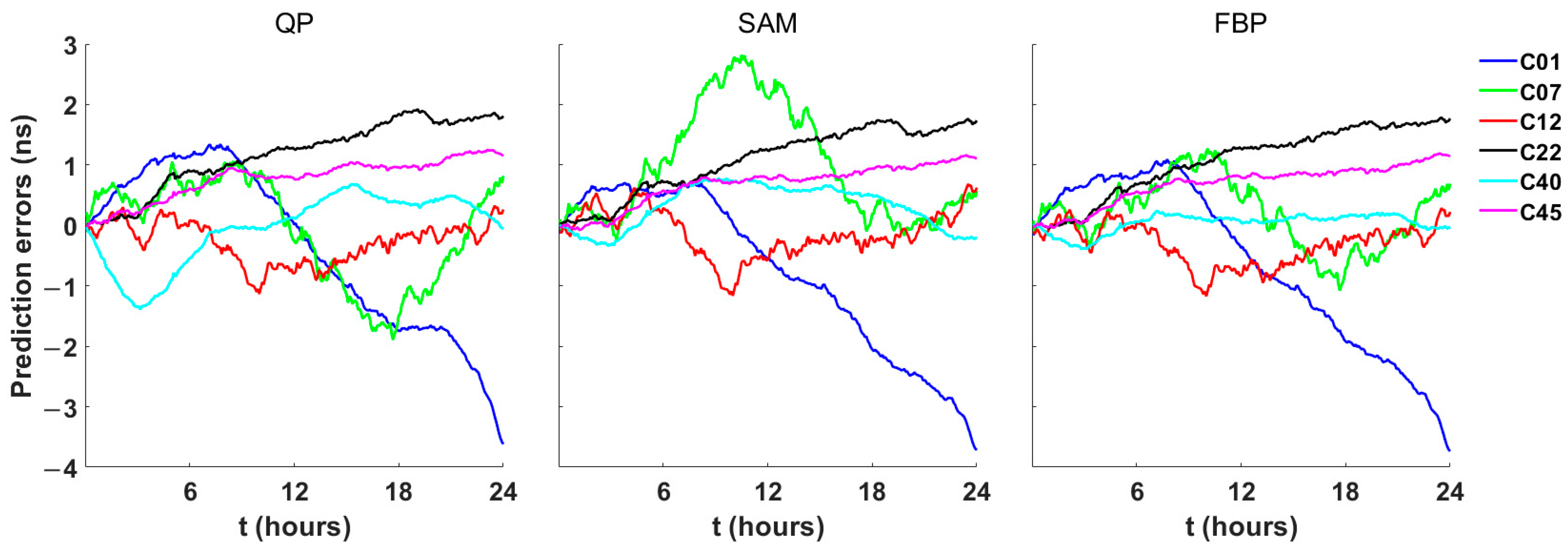
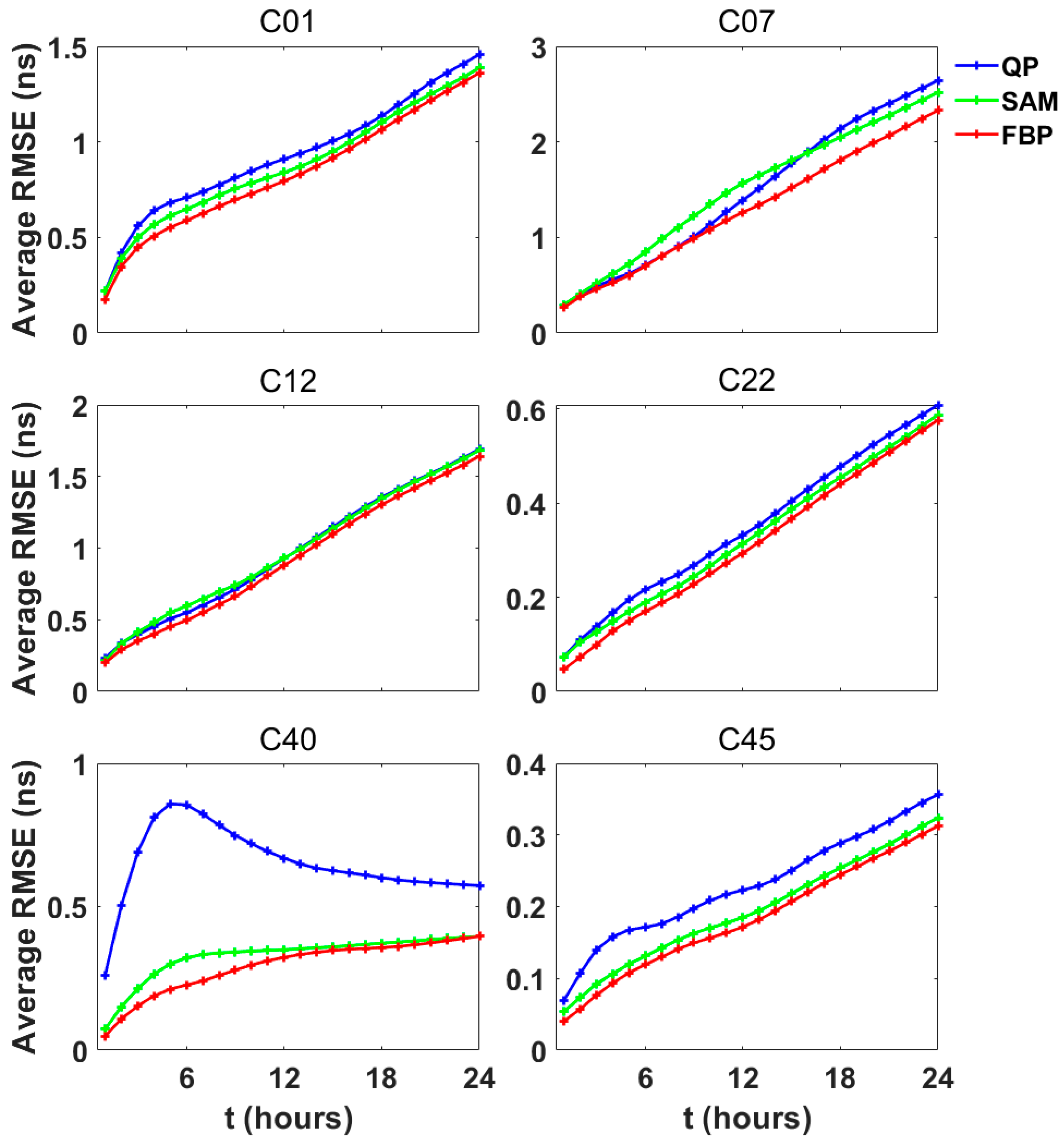
4.3. Clock Prediction Analysis of the BDS Satellite Clocks

To validate the capability of the FBPBPF method in extracting periodic terms through simulation experiments, this study employs the QP prediction method, the SAM prediction method based on LSM and the FBP prediction method based on FBPBPF to predict the clock bias data of BDS satellites listed in Table 2. The specific steps are as follows: First, since extracting periodic terms with period of 24 h usually requires at least 48 h of data, in order to balance the accuracy and efficiency of clock bias prediction, 72 h of clock bias data is used to fit the prediction model, and the model is used to predict the clock bias for the next 24 h. Then, the prediction is continued for 25 days, and each time the predicted value is compared with the measured clock bias data and the root mean square error (RMSE) of the prediction error from 1 to 24 h per day is calculated. The prediction error on February 8, 2023, is shown in Figure 7. The average RMSE of the 1 to 24 h over the 25 predictions is shown in Figure 8. By comparing the prediction results of QP, SAM and FBP, the improvement in the prediction accuracy of the FBP prediction method at different time intervals (6 h, 12 h, 18 h and 24 h) is evaluated, as shown in

Table 3. The average RMSE of the QP, the SAM and the FBP prediction errors at 6, 12, 18 and 24 h.

PRN	6 h (ns)			12 h (ns)			18 h (ns)			24 h (ns)
	QP	SAM	FBP	QP	SAM	FBP	QP	SAM	FBP	QP	SAM	FBP
C01	0.709	0.648	0.588	0.910	0.839	0.794	1.136	1.103	1.065	1.457	1.388	1.361
C07	0.708	0.845	0.699	1.391	1.568	1.262	2.141	2.050	1.810	2.643	2.516	2.328
C12	0.548	0.595	0.495	0.928	0.929	0.880	1.355	1.346	1.303	1.690	1.682	1.642
C22	0.216	0.189	0.169	0.332	0.313	0.293	0.478	0.454	0.440	0.609	0.587	0.576
C40	0.854	0.321	0.227	0.668	0.349	0.322	0.600	0.371	0.356	0.573	0.395	0.395
C45	0.171	0.130	0.118	0.223	0.184	0.171	0.288	0.254	0.244	0.356	0.323	0.312
Avg.	0.534	0.454	0.382	0.742	0.697	0.620	0.999	0.929	0.869	1.221	1.148	1.102

.

The experimental results show that the FBP prediction method effectively suppresses the periodic fluctuations in prediction errors for satellites with significant periodic variations (such as C07 and C40), as shown in Figure 7 and significantly reduces the overall prediction errors, as shown in Figure 8. In contrast, due to the shorter model fitting time, the SAM prediction method exhibits relatively weaker modeling accuracy for periodic components, resulting in residual periodic fluctuations in its prediction errors, and even lower accuracy than QP in some time periods (such as C07 and C12). This further demonstrates that the FBPBPF method achieves higher accuracy in extracting periodic terms at the signal boundaries, especially under conditions of strong noise interference.

As shown in Table 3, compared to the QP and the SAM, the FBP prediction method significantly improves prediction accuracy across all time intervals and the improvement is more significant in shorter time intervals (6 h). For predictions over 6, 12, 18, and 24 h, the average RMSE of the FBP prediction method is reduced by 28.46%, 16.44%, 13.01%, and 9.74%, respectively, relative to QP. Among these, the satellite with significant periodic variations (such as C40) achieved a remarkable reduction of 73.41% in RMSE for 6 h predictions, demonstrating outstanding performance. Compared with SAM, the average RMSE of the FBP prediction method is reduced by 15.85%, 11.04%, 6.45% and 4.01%, respectively.

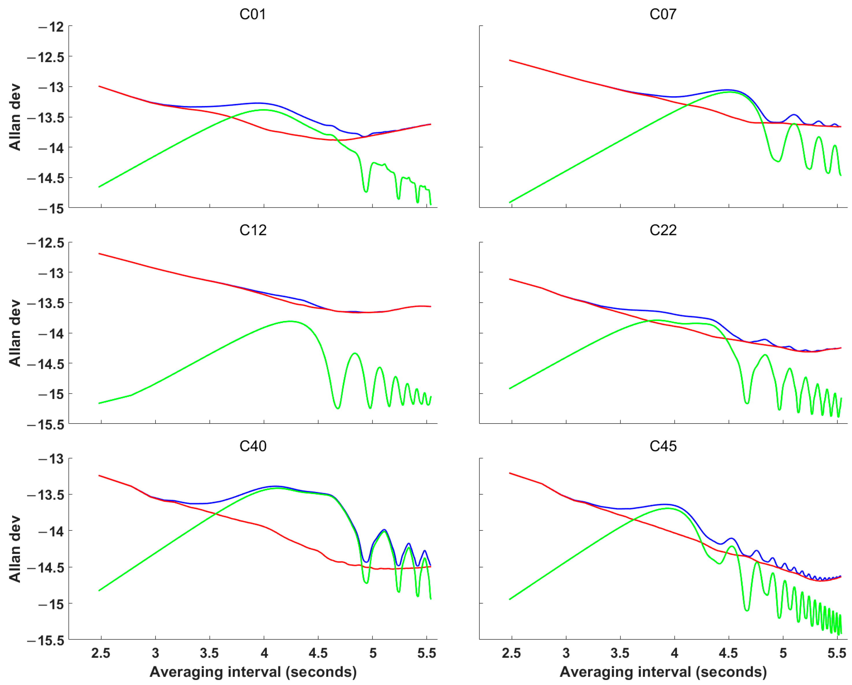
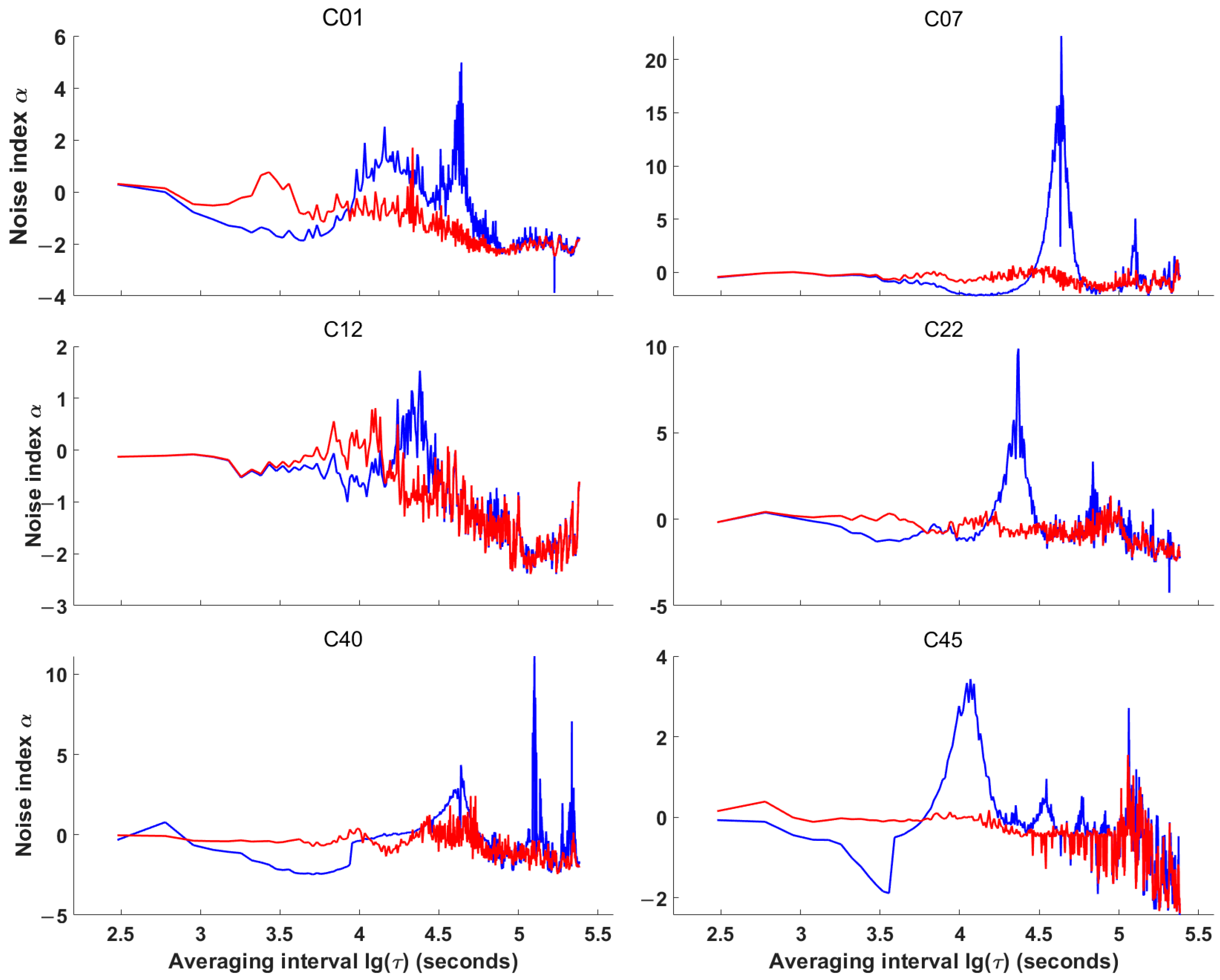
4.4. Frequency Stability Analysis and Noise Type Identification

To verify the accuracy and effectiveness of FBPBPF in extracting periodic terms from clock bias data, the main periodic terms were extracted as listed in Table 2. Frequency stability curves and lag 1 autocorrelation function (ACF) noise type [38,39] were plotted before and after periodic term correction, as shown in Figure 9 and Figure 10. The Allan deviation (with the clock bias trend removed) was used to calculate frequency stability, and the periodic term extraction method was evaluated based on improvements in frequency stability at averaging times of 10,000 s, 20,000 s, and 40,000 s, along with suppression of oscillatory peaks.

As shown in Figure 9, the Allan deviation curve becomes smoother after the periodic term correction, indicating that removing the periodic terms from the clock bias effectively suppresses the anomalous peaks and oscillations present in the original frequency stability curve. The FBPBPF significantly enhances the stability at each smoothing interval. Specifically, for averaging times of 10,000 s, 20,000 s, and 40,000 s, the frequency stability is improved by an average of 42.7%, 46.6%, and 38.5%, respectively, over the original data. Notably, the frequency stability improvement for C12 is the lowest, likely due to high atomic clock noise. These results show that the FBPBPF effectively reduces oscillatory peaks in the original Allan deviation curve, and the degree of improvement in frequency stability is closely related to factors such as satellite system type, onboard clock type, and satellite orbit.

As shown in Figure 10, the noise type of the BDS satellite clock changes as the smoothing time increases. However, in general, the BDS satellite clock is mainly affected by white frequency modulation noise, flicker frequency modulation noise, and random walk frequency modulation noise. The BDS satellite clock before the periodic term is extracted has a large noise index in the smoothing time range of 5000 s to 50,000 s. The reason for the large fluctuations is that its clock bias data have a more pronounced periodicity. After the periodic term is eliminated using an FBPBPF, the abnormal fluctuations in the lag 1 ACF noise type in the longer smoothing time range are effectively suppressed, and its original noise characteristics are revealed.

5. Conclusions

This study analyzed the impact of periodic terms in satellite clock bias on the performance analysis of atomic clocks, highlighted the importance of extracting these terms, and introduced the FBP spectrum and the FBPBPF-based method for extracting periodic terms in clock bias. Analysis of simulated satellite clock bias data demonstrated that the FBPBPF achieves superior noise suppression and accuracy in extracting time-varying periodic terms compared to the LSM, FIR, and IIR methods. Specifically, compared to the LSM, FIR, and IIR, the FBPBPF reduces the entire extraction error by an average of 6.81%, 19.96%, and 26.55%, respectively, and reduces the extraction error at the boundaries by an average of 11.47%, 63.67%, and 60.63%, respectively, demonstrating a significant advantage in mitigating boundary effects. Compared to the SAM, the FBP prediction method significantly improves prediction accuracy across all time intervals, as verified using WHU satellite clock bias data. For predictions over 6, 12, 18, and 24 h, the average RMS errors of the FBP prediction method are reduced by 15.85%, 11.04%, 6.45%, and 4.01%, respectively.

The time-frequency characteristics of the satellite clock bias were analyzed using FBP-based STFT. Since the FBP spectrum is superior to the rectangular, Hanning and Blackman windows in terms of reducing spectral leakage, in addition to the 24 h, 12 h and 6 h periodic terms commonly found in BDS satellite clock bias, periodic terms of 8 h, 20 h and 28 h periodic terms were additionally found for certain satellites. Through a comparative analysis of the lag 1 ACF noise type before and after the correction of the periodic term, it was identified that the periodic term is the main factor driving the abnormal fluctuations in the noise index. A comparative analysis of the frequency stability before and after the periodic term correction revealed that abnormal peaks and oscillations in the original frequency stability curve were effectively suppressed after the correction, confirming the accuracy and effectiveness of the FBPBPF in extracting periodic terms from the clock bias. After the periodic term correction, the satellite clock frequency stability improved significantly, with enhancements of 42.7%, 46.6%, and 38.5% at 10,000 s, 20,000 s, and 40,000 s averaging times, respectively. These improvements help to accurately analyze the performance of the spaceborne atomic clock.

References

1. Xie, X.; Geng, T.; Zhao, Q.; Lv, Y.; Cai, H.; Liu, J. Orbit and Clock Analysis of BDS-3 Satellites Using Inter-Satellite Link Observations. J. Geod. 2020, 94, 64. [Google Scholar] [CrossRef]
2. Sun, L.; Huang, W.; Gao, S.; Li, W.; Guo, X.; Yang, J. Joint Timekeeping of Navigation Satellite Constellation with Inter-Satellite Links. Sensors 2020, 20, 670. [Google Scholar] [CrossRef] [PubMed]
3. Senior, K.L.; Ray, J.R.; Beard, R.L. Characterization of Periodic Variations in the GPS Satellite Clocks. GPS Solut. 2008, 12, 211–225. [Google Scholar] [CrossRef]
4. Formichella, V.; Galleani, L.; Signorile, G.; Sesia, I. Time–Frequency Analysis of the Galileo Satellite Clocks: Looking for the J2 Relativistic Effect and Other Periodic Variations. GPS Solut. 2021, 25, 56. [Google Scholar] [CrossRef]
5. Galleani, L.; Tavella, P. The Dynamic Allan Variance V: Recent Advances in Dynamic Stability Analysis. IEEE Trans. Ultrason. Ferroelectr. Freq. Control 2016, 63, 624–635. [Google Scholar] [CrossRef] [PubMed]
6. Heo, Y.J.; Cho, J.; Heo, M.B. Improving Prediction Accuracy of GPS Satellite Clocks with Periodic Variation Behaviour. Meas. Sci. Technol. 2010, 21, 073001. [Google Scholar] [CrossRef]
7. Cao, Y.; Huang, G.; Xie, S.; Xie, W.; Liu, Z.; Tan, Y. An Evaluation Method of GPS Satellite Clock In-Orbit with Periodic Terms Deducted. Measurement 2023, 214, 112765. [Google Scholar] [CrossRef]
8. Zhao, L.; Li, N.; Li, H.; Wang, R.; Li, M. BDS Satellite Clock Prediction Considering Periodic Variations. Remote Sens. 2021, 13, 4058. [Google Scholar] [CrossRef]
9. Galleani, L. Detection of Changes in Clock Noise Using the Time–Frequency Spectrum. Metrologia 2008, 45, S143. [Google Scholar] [CrossRef]
10. Wang, G.; Liu, L.; Xu, A.; Pan, F.; Cai, Z.; Xiao, S.; Tu, Y.; Li, Z. On the Capabilities of the Inaction Method for Extracting the Periodic Components from GPS Clock Data. GPS Solut. 2018, 22, 92. [Google Scholar] [CrossRef]
11. Huang, N.E.; Shen, Z.; Long, S.R.; Wu, M.C.; Shih, H.H.; Zheng, Q.; Yen, N.-C.; Tung, C.C.; Liu, H.H. The Empirical Mode Decomposition and the Hilbert Spectrum for Nonlinear and Non-Stationary Time Series Analysis. Proc. R. Soc. Lond. Ser. A Math. Phys. Eng. Sci. 1998, 454, 903–995. [Google Scholar] [CrossRef]
12. Lv, Y.; Dai, Z.; Zhao, Q.; Yang, S.; Zhou, J.; Liu, J. Improved Short-Term Clock Prediction Method for Real-Time Positioning. Sensors 2017, 17, 1308. [Google Scholar] [CrossRef] [PubMed]
13. Wang, W.; Wang, Y.; Yu, C.; Xu, F.; Dou, X. Spaceborne Atomic Clock Performance Review of BDS-3 MEO Satellites. Measurement 2021, 175, 109075. [Google Scholar] [CrossRef]
14. Wang, L.; Bi, G.; Lv, X. Analysis of Sidelobe Effects and Resolution of PTFT. In Proceedings of the 2011 9th IEEE International Conference on Control and Automation (ICCA), Santiago, Chile, 19–21 December 2011; pp. 1049–1054. [Google Scholar]
15. Guo, T.; Zhang, T.; Lim, E.; López-Benítez, M.; Ma, F.; Yu, L. A Review of Wavelet Analysis and Its Applications: Challenges and Opportunities. IEEE Access 2022, 10, 58869–58903. [Google Scholar] [CrossRef]
16. Yifeng, L.; Jiangning, X.; Fangneng, L.; Miao, W. A VMD-PE-SG Denoising Method Based on K–L Divergence for Satellite Atomic Clock. Meas. Sci. Technol. 2023, 34, 055012. [Google Scholar] [CrossRef]
17. Kim, J.K.; Ahn, J.M. Effects of a Spectral Window on Frequency Domain HRV Parameters. In Advances in Computer Communication and Computational Sciences; Bhatia, S.K., Tiwari, S., Mishra, K.K., Trivedi, M.C., Eds.; Springer: Singapore, 2019; pp. 697–710. [Google Scholar]
18. Özhan, O. Short-Time-Fourier Transform. In Basic Transforms for Electrical Engineering; Özhan, O., Ed.; Springer International Publishing: Cham, Switzerland, 2022; pp. 441–464. ISBN 978-3-030-98846-3. [Google Scholar]
19. Kumar, K.S.; Yazdanpanah, B.; Kumar, P.R. Removal of Noise from Electrocardiogram Using Digital FIR and IIR Filters with Various Methods. In Proceedings of the 2015 International Conference on Communications and Signal Processing (ICCSP), Melmaruvathur, India, 2–4 April 2015; pp. 0157–0162. [Google Scholar]
20. Rabiner, L.R.; Kaiser, J.F.; Herrmann, O.; Dolan, M.T. Some Comparisons Between FIR and IIR Digital Filters. Bell Syst. Tech. J. 1974, 53, 305–331. [Google Scholar] [CrossRef]
21. Wang, G.; Liu, L.; Su, X.; Liang, X.; Yan, H.; Tu, Y.; Li, Z.; Li, W. Variable Chandler and Annual Wobbles in Earth’s Polar Motion During 1900–2015. Surv. Geophys. 2016, 37, 1075–1093. [Google Scholar] [CrossRef]
22. Olshausen, B.; Sallee, P.; Lewicki, M. Learning Sparse Image Codes Using a Wavelet Pyramid Architecture. In Advances in Neural Information Processing Systems; MIT Press: Cambridge, MA, USA, 2000; Volume 13. [Google Scholar]
23. Starck, J.-L.; Elad, M.; Donoho, D.L. Image Decomposition via the Combination of Sparse Representations and a Variational Approach. IEEE Trans. Image Process. 2005, 14, 1570–1582. [Google Scholar] [CrossRef]
24. Li, Y.; Cichocki, A.; Amari, S. Analysis of Sparse Representation and Blind Source Separation. Neural Comput. 2004, 16, 1193–1234. [Google Scholar] [CrossRef] [PubMed]
25. Elad, M.; Aharon, M. Image Denoising Via Learned Dictionaries and Sparse Representation. In Proceedings of the 2006 IEEE Computer Society Conference on Computer Vision and Pattern Recognition (CVPR’06), New York, NY, USA, 17–22 June 2006; Volume 1, pp. 895–900. [Google Scholar]
26. Gao, F.; Wang, G.; Liu, L.; Xu, H.; Liang, X.; Shi, Z.; Ren, D.; Hu, H.; Sun, X. Tidal Analysis and Prediction Based on the Fourier Basis Pursuit Spectrum. Ocean. Eng. 2023, 278, 114414. [Google Scholar] [CrossRef]
27. Mallat, S.G.; Zhang, Z. Matching Pursuits with Time-Frequency Dictionaries. IEEE Trans. Signal Process. 1993, 41, 3397–3415. [Google Scholar] [CrossRef]
28. Chen, S.S.; Donoho, D.L.; Saunders, M.A. Atomic Decomposition by Basis Pursuit. SIAM J. Sci. Comput. 1998, 20, 33–61. [Google Scholar] [CrossRef]
29. Daubechies, I. Time-Frequency Localization Operators: A Geometric Phase Space Approach. IEEE Trans. Inf. Theory 1988, 34, 605–612. [Google Scholar] [CrossRef]
30. Baraniuk, R.G.; Jones, D.L. Shear Madness: New Orthonormal Bases and Frames Using Chirp Functions. IEEE Trans. Signal Process. 1993, 41, 3543–3549. [Google Scholar] [CrossRef]
31. Mihovilovic, D.; Bracewell, R.N. Adaptive Chirplet Representation of Signals on Time–Frequency Plane. Electron. Lett. 1991, 27, 1159. [Google Scholar] [CrossRef]
32. Mallat, S. A Wavelet Tour of Signal Processing; Elsevier: Amsterdam, The Netherlands, 1999; ISBN 978-0-12-466606-1. [Google Scholar]
33. Chen, S.; Donoho, D. Basis Pursuit. In Proceedings of the 1994 28th Asilomar Conference on Signals, Systems and Computers, Pacific Grove, CA, USA, 31 October–2 November 1994; Volume 1, pp. 41–44. [Google Scholar]
34. Tary, J.B.; Herrera, R.H.; Han, J.; Van Der Baan, M. Spectral Estimation-What Is New? What Is Next? Rev. Geophys. 2014, 52, 723–749. [Google Scholar] [CrossRef]
35. Liang, Y.; Xu, J.; Wu, M.; Li, F. Analysis of the Long-Term Characteristics of BDS On-Orbit Satellite Atomic Clock: Since BDS-3 Was Officially Commissioned. Remote Sens. 2022, 14, 4535. [Google Scholar] [CrossRef]
36. Höpfner, J. Low-Frequency Variations, Chandler and Annual Wobbles of Polar Motion as Observed Over One Century. Surv. Geophys. 2004, 25, 1–54. [Google Scholar] [CrossRef]
37. Wu, J. Study on Detection of GPS Clock Jump Using Median Absolute Deviation. Sci. Surv. Mapp. 2015, 40, 36–41. [Google Scholar] [CrossRef]
38. Ai, Q.; Maciuk, K.; Lewinska, P.; Borowski, L. Characteristics of Onefold Clocks of GPS, Galileo, BeiDou and GLONASS Systems. Sensors 2021, 21, 2396. [Google Scholar] [CrossRef]
39. Riley, W.J.; Greenhall, C.A. Power Law Noise Identification Using the Lag 1 Autocorrelation. In 2004 18th European Frequency and Time Forum (EFTF 2004); IEE: Stevenage, UK, 2004; pp. 576–580. [Google Scholar]
Figure 1. Simulated satellite clock bias. (a) the amplitude of periodic term; (b) time domain of periodic term; (c) time domain of mixed signal and noise; (d) Allan deviation of the simulated signal.
Remotesensing 17 00827 g001
Figure 2. The spectrum of the simulated clock bias calculated using windowed Fourier transform and Fourier basis pursuit (FBP). As the Hanning and Blackman windows introduce amplitude distortions, corresponding window function compensation factors are applied. For clearer analysis of periodic phenomena in the time series, the frequency axis is converted to the period axis. (a) the spectrum of FBP; (b) the spectrum based on rectangular window; (c) the spectrum based on Hanning window; (d) the spectrum based on Blackman window.
Remotesensing 17 00827 g002
Figure 3. Simulated 6 h periodic term (blue), reconstructed 6 h periodic term (green), and extraction residual (red). The simulated data are divided into five segments; each row in the figure represents the experimental results for one of these time series segments, and each column represents a different method for extracting the periodic terms. (a,e,i,m,q) extracting periodic term with LSM; (b,f,j,n,r) extracting periodic term with FBPBPF; (c,g,k,o,s) extracting periodic term with FIR; (d,h,l,p,t) extracting periodic term with IIR.
Remotesensing 17 00827 g003
Figure 4. Simulated 12 h periodic term (blue), reconstructed 12 h periodic term (green), and extraction residual (red). The simulated data are divided into five segments; each row in the figure represents the experimental results for one of these time series segments, and each column represents a different method for extracting the periodic term. (a,e,i,m,q) extracting periodic term with LSM; (b,f,j,n,r) extracting periodic term with FBPBPF; (c,g,k,o,s) extracting periodic term with FIR; (d,h,l,p,t) extracting periodic term with IIR.
Remotesensing 17 00827 g004
Figure 5. Simulated 24 h periodic term (blue), reconstructed 24 h periodic term (green), and extraction residual (red). The simulated data are divided into five segments; each row in the figure represents the experimental results for one of these time series segments, and each column represents a different method for extracting the periodic term. (a,e,i,m,q) extracting periodic term with LSM; (b,f,j,n,r) extracting periodic term with FBPBPF; (c,g,k,o,s) extracting periodic term with FIR; (d,h,l,p,t) extracting periodic term with IIR.
Remotesensing 17 00827 g005
Figure 6. Time-frequency spectrum of the BDS satellite clock bias. (a) the spectrum of C01; (b) the spectrum of C22. In the experiment, the window width and the overlap ratio of the STFT are kept constant for all methods. The amplitude distortion introduced by the Hanning and Blackman windows is compensated by the corresponding window function recovery factors. Each row represents the experimental results for the same satellite clock, and each column represents a different spectral analysis method. To facilitate intuitive analysis of periodic phenomena in the time series, the frequency axis is converted to a period axis.
Remotesensing 17 00827 g006
Figure 7. The prediction errors of the BDS satellite clocks on 8 February 2023.
Remotesensing 17 00827 g007
Figure 8. The average RMSE of the QP, the SAM and the FBP prediction errors from 1 to 24 h.
Remotesensing 17 00827 g008
Figure 9. Allan deviation l g σ y τ ~ l g τ before and after periodic term correction. τ is the averaging time interval. The blue line represents the Allan deviation of the original clock bias, the green line represents the Allan deviation of the extracted periodic terms, and the red line represents the Allan deviation after periodic term correction using FBPBPF.
Remotesensing 17 00827 g009
Figure 10. The lag 1 ACF noise type before and after periodic term correction. τ is the averaging time interval. The blue line represents the lag 1 ACF of the original clock bias and the red line represents the lag 1 ACF after periodic term correction using FBPBPF.
Remotesensing 17 00827 g010