Progress in Atmospheric Density Inversion Based on LEO Satellites and Preliminary Experiments for SWARM-A

Abstract

The vigorous development of Low Earth Orbit (LEO) satellite constellation programs imposes higher requirements for the accuracy of satellite orbit determination. Significant variations in atmospheric density within the operational region of LEO satellites are primary factors influencing their orbital decay and operational lifespan. This article first summarizes the research advancements in atmospheric density inversion utilizing LEO satellites, comparing and analyzing the principles of various algorithms, factors affecting accuracy, as well as the advantages and disadvantages associated with different acquisition methods. Subsequently, we introduce recent progress in enhancing atmospheric density inversion algorithms and data analysis applications based on LEO satellites. The SWARM-A satellite, equipped with a high-precision GPS receiver and accelerometer, was employed to invert atmospheric density using both semi-long axis attenuation and accelerometer methodologies. The inversion results were compared against empirical models to validate their reliability; specifically, the correlation coefficient between the semi-long axis attenuation method and nrlmsise00 reached 0.9158, while that between the accelerometer method and nrlmsise00 attained 0.9204. Notably, the inversion accuracy achieved by the accelerometer slightly surpasses that of the semi-long axis attenuation method. These findings provide valuable support for predicting large air tightness based on LEO satellite orbit data inversions and for adjusting operational orbits to ensure successful execution of satellite missions.

1. Introduction

The term “Low Earth Orbit (LEO)” satellites is commonly used to refer to satellites that traverse the Earth’s surface at altitudes ranging from approximately 80–100 km [1] to 2000 km [2]. Within this altitude range, LEO satellites demonstrate reduced signal latency and enhanced signal strength [3], which provide significant advantages in various fields such as communications, weather monitoring, and remote sensing observations. In recent years, the deployment of LEO satellite constellations by commercial aerospace companies including SpaceX’s Starlink program, OneWeb, and Amazon [4,5,6,7,8] has resulted in a substantial increase in both the number of operational LEO satellites and the frequency of their launches [9]. The utilization of data from LEO satellites allows researchers to observe the Earth’s surface in real-time. This capability offers a scientific foundation for monitoring space weather as well as guiding satellite navigation and climate modeling. Within the Earth’s magnetosphere, where LEO satellites operate, highly reactive atomic oxygen constitutes approximately 80% or more of the total atmospheric composition. This component exhibits a strong absorptive capacity for solar radiation [10], thus meaning that normal operations of LEO satellites are directly influenced by solar activity affecting both the atmosphere and ionosphere. Increases in solar activity lead to radiation production by energetic particles within the solar wind, and this phenomenon subsequently impacts payload service life [11]. Moreover, variations in space weather can induce changes in atmospheric density that affect orbital stability for LEO satellites. Such alterations may result in decreased altitude and slowed operational velocity. During periods characterized by heightened solar activity, a denser atmosphere not only accelerates orbital decay but also diminishes operational lifespan while weakening communication signals and causing delays in signal transmission. This has a significant impact on the accuracy of communication and positioning [12].

A search of 5776 research articles in the Web of Science (WOS) using the keywords ’LEO satellites’ and ’Low Earth Orbit satellites’ revealed several pertinent keywords. A keyword co-occurrence, clustering, and emergence analysis indicates that ’orbit’ is the most frequently occurring keyword (Figure 1), establishing it as a core focus within this satellite field of research. The gravitational influences of the Sun and Moon, solar activity, and light pressure all play a crucial role in determining the stability of Low Earth Orbit (LEO) satellite operations. Furthermore, variations in solar activity can alter the forces acting on satellites by modifying atmospheric density. During a magnetic storm, LEO satellites with different orbital inclination and orbital height are affected by levels of different atmospheric drag, and LEO satellites with smaller orbital inclinations are affected by greater resistance, which increases the possibility of collision between satellites [13]. Fluctuations in atmospheric density necessitate regular orbital adjustments to mitigate excessive atmospheric drag, which could otherwise result in satellite destruction. Changes in atmospheric composition will also lead to large signal noise and time delay, which will have an impact on real-time navigation and emergency rescue.

Accurate atmospheric density inversion not only enhances existing climate and weather prediction models but also optimizes Low Earth Orbit satellite orbit design and mission execution based on dynamic changes, thereby improving the success rate of missions. There are two primary algorithms for atmospheric density inversion utilizing LEO satellites: The first algorithm involves indirectly calculating the mean atmospheric drag force acceleration using orbital data from LEO satellites, in conjunction with satellite attitude and material properties as dictated by a dynamics model [14,15]. This approach further facilitates the inversion of atmospheric density, allowing for comparison with traditional empirical models such as NRLMISISE-00 and DTM to validate the results. While this method is straightforward and computationally efficient, it faces challenges in practical satellite operations. Atmospheric density is closely linked to solar radiation, variations in the Earth’s magnetic field, intrinsic atmospheric activity, and the Earth’s rotation [16]. The unpredictability of changes in solar radiation and the Earth’s magnetic field affects the drag coefficient experienced by satellites over time, and current predictive accuracy falls short of meeting the stringent requirements for high-precision space missions involving space rendezvous operations, collision warnings, and precision tracking. In response to this challenge, scientists have developed methods to directly measure the non-conservative absorption force on satellites using highly accurate onboard accelerometers [17]. Through the integration of data from multiple satellite accelerometers like CHAMP, GRACE, and SWARM, among others, the scientists improved the accuracy of calibration and determined the immediate acceleration of atmospheric drag forces on satellites during their operation for atmospheric density inversion [18,19,20]. The inaccuracies in accelerometer readings due to sensor hardware variances remain unresolved, necessitating further enhancements in data precision. Additionally, the frequency of data updates is relatively low, leading to considerable delays, and the consequent inversion error is also substantial.

The global Low Earth Orbit satellites program is currently experiencing substantial growth, with an unprecedented number of satellite launches providing a robust dataset for scientific experimentation. However, there has been a marked decline in the availability of atmospheric density products derived from LEO satellite data. To evaluate the feasibility of utilizing LEO satellite data for atmospheric density inversion and to address challenges related to low precision in satellite orbit determination and significant delays in orbit prediction adjustments, we conducted a two-part study as follows. The first part encompasses research advancements regarding atmospheric density inversion based on Low Earth Orbit satellites. This includes methods for acquiring atmospheric density from these satellites, presented in Section 2, and progress made in atmospheric density inversion, discussed in Section 3. The second part involves an experimental investigation into atmospheric density inversion utilizing SWARM-A data. This example illustrates the viability of employing LEO satellite data for atmospheric density inversion while laying the groundwork for algorithm enhancements aimed at improving inversion accuracy and generating high-quality atmospheric density products based on extensive LEO satellite datasets. The acquisition of high-precision atmospheric density data are of paramount importance for the accurate prediction of satellite orbits. This can significantly reduce the impact of orbital decay on satellite life, thereby guaranteeing the safety of LEO satellite launches and operations. It provides data support for atmospheric density modeling, thus improving the accuracy of the model [21]. It is of great significance for monitoring changes in space weather and evaluating extreme weather conditions [22].

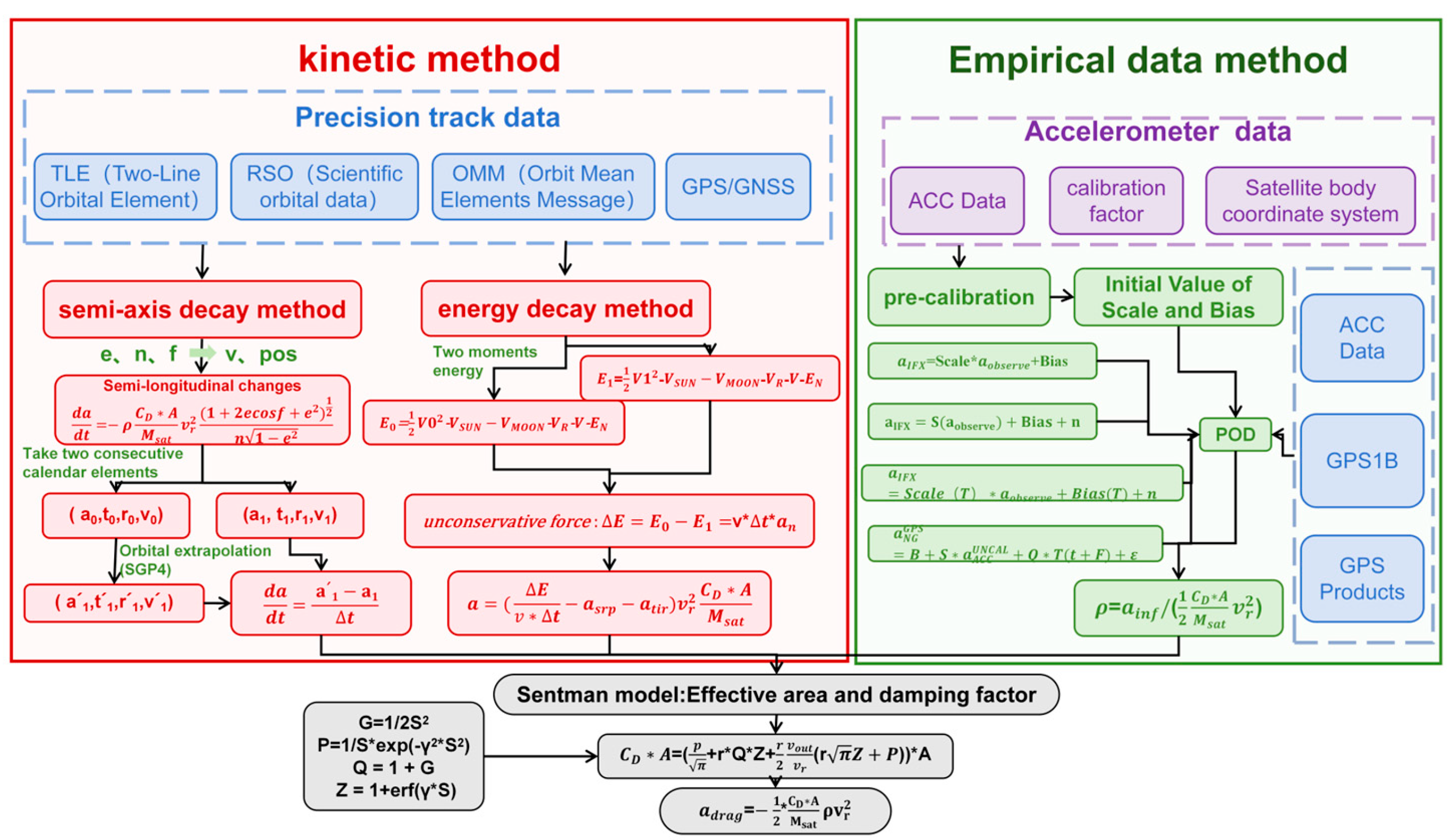
2. Methods of Atmospheric Density Inversion for Low Earth Orbit Satellites

Atmospheric density inversion is classified into three categories based on the data source used to calculate the drag force [23]. The first method involves obtaining the atmospheric density by detecting temperature, humidity, and pressure in the atmosphere using sensors carried by aerospace instruments. Notable examples include China’s Shenzhou series and Tiangong series spacecraft. In addition to the direct detection of atmospheric density with physical detectors, we can also use the changes in relevant parameters caused by atmospheric drag force during the operation of LEO satellites to calculate the atmospheric density. The second method entails calculating the attenuation of the half-length axis of the orbit or the change in the overall energy of the satellite based on satellite orbital data, thereby indirectly calculating the atmospheric drag force on the satellite and inverting the atmospheric density. The third method involves calculating the atmospheric density directly after calibrating the acquired onboard accelerometer data. Either method necessitates the calculation of the atmospheric drag force, the atmospheric damping coefficient, and the effective cross-sectional area.

2.1. Calculation of Atmospheric Drag Force

In the Low Earth Orbit (LEO) operating region, the interaction of the spacecraft with the atmosphere is predominantly characterized by free molecular flow [24]. This interaction results in the spacecraft being subjected to a drag force; the formula is provided in the following Equation (1). Based on the following equation, the drag force is calculated and then combined with the mass of the spacecraft and the atmospheric damping coefficient, $C_D$, which is estimated based on parameters such as its morphology, attitude, and panel material. This information can be obtained from official data center. Synthesizing the above information, this allows the atmospheric density to be calculated.

$$a_{drag}=-{\displaystyle \frac{1}{2}}\ast {\displaystyle \frac{C_D\ast A}{M_{sat}}}\rho v_r^2$$

(1)

The graphene $A$ serves to represent the corresponding cross-sectional area of the orbital trajectory of the spacecraft. While the letter $M_{sat}$ denotes the mass of the satellite, $C_D$ represents the atmospheric damping coefficient, and $C_D\ast A$ is the ballistic coefficient, which represents the characteristics of the satellite’s surface. $v_r$ denotes the velocity of the spacecraft relative to the atmosphere, and $\rho$ denotes the atmospheric mass density in the thermosphere near the spacecraft [25,26,27].

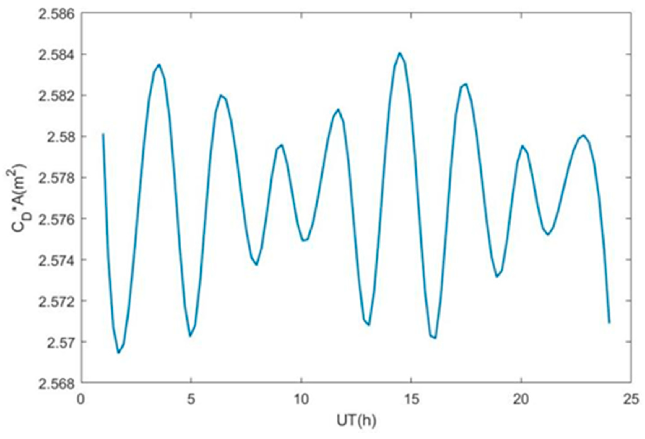
2.2. Product of Atmospheric Damping Coefficient and Effective Area

As atmospheric molecules interact with each satellite panel, a drag effect is observed. The atmospheric drag force on each satellite panel is initially calculated, and the total drag force on all panels is superimposed. The atmospheric damping coefficient, $C_D$, is calculated using the Sentman model [26], as detailed in the following formula.

$$C_D\ast A=[{\displaystyle \frac{P}{\sqrt{\pi }}}+\gamma QZ+{\displaystyle \frac{\gamma }{2}}{\displaystyle \frac{v_{out}}{v_{at}}}(\gamma \sqrt{\pi }Z+P\left)\right]\ast A$$

(2)

The ratio $S$ is equal to the thermodynamically best-distributed velocity of the atmospheric molecules. The symbol $P$ is equal to ${\displaystyle \frac{1}{S\ast \mathrm{e}\mathrm{x}\mathrm{p}(-{\gamma }^2\ast S^2)}}$, $G$ represents a value of ${\displaystyle \frac{1}{2S^2}}$, $Q$ is equal to $1+G$, and $Z$ is equal to $1+\mathrm{e}\mathrm{r}\mathrm{f}(\gamma \ast S)$. The symbol $\gamma$ denotes the cosine of the angle normal to the incident atmospheric molecular flow and the satellite panel. The term $v_{out}$ denotes the velocity of the atmospheric molecular flow after collision with the satellite panel, while $v_{at }$ represents the atmospheric velocity in relative terms for the satellite [18].

$${\displaystyle \frac{v_{out}}{v_{at}}}=\sqrt{{\displaystyle \frac{2}{3}}[1+{\alpha }_E({\displaystyle \frac{T_{wall}}{T_{in}}}-1\left)\right]}$$

(3)

The character $T_{in}$ is defined as the molecular dynamics temperature of the incident atmosphere, represented by the equation ${\displaystyle \frac{(m_a\ast v_{at}^2)}{3R}}$, where $R$ can be defined as a constant equal to 8314 J/mol. $K$ is a thermodynamic constant, and $m_a$ is equal to the average relative molecular mass of the atmosphere. The value of $T_{wall}$ indicates that the temperature of the spacecraft panel is assumed to be 300 K. The energy exchange efficiency between the incident atmospheric molecular flow and the spacecraft panel, represented by ${\alpha }_E$, is equal to 0.93 [19].

$$S={\displaystyle \frac{v_{at}}{\sqrt{2RT/m_a}}}$$

(4)

The atmospheric damping coefficient can be reduced to a functional equation that is solely dependent on the temperature $T$, the mean relative molecular mass of the atmosphere denoted by the symbol $m_a$, and so forth. $T$ represents the local temperature of the atmosphere, which must be determined through empirical model calculations.

2.3. Comparison of Three Inversion Methods

According to the classification results of atmospheric density acquisition methods in

Table 1. Comparison of three methods for obtaining atmospheric density, based on these methods’ principles, accuracy-influencing factors, and applicable situations in different environments for obtaining atmospheric density.

Method	Sensor Detections	Precision Orbits		Accelerometer Data
Theory	Instrument detection	Semi-long axis attenuation	Conservation of mechanical energy	Acceleration calibration
Data	Atmospheric density	Positional velocity	Gravity field model Gravitational potential	Scale, bias, and temperature factors
Factors affecting accuracy	Atmospheric environment signal source	Quality and period of orbital data	Model assumptions and parameter	Instrument noise and error
Conditions of application	Widespread monitoring	Long-term monitoring and large-scale	Scenes of high-precision inversion	Real-time monitoring and dynamic inversion

, a comparative analysis is conducted from the aspects of acquisition principle, inversion process, required data, and method advantages. The instrument detection method derives atmospheric density from parameters such as temperature, humidity, and barometric pressure through sensors integrated into aviation equipment. Gradiometers and atmospheric density probes, such as those carried on low-orbiting satellites, are capable of covering a large area of the Earth’s surface and detecting it at high altitudes, directly acquiring atmospheric density, but the launch and maintenance costs are high, and there may be time delays in data processing and transmission, which affects the ability to monitor it in real-time.

The inversion of atmospheric density from precision orbital data provided by satellites includes two methods, the half-length axis decay method and the energy conservation method. In Low Earth Orbit satellite operation, atmospheric drag force results in orbit height decline, usually with the satellite half-length axis of the change in the description of the orbit height change [28], and the half-length axis with the rate of change of time directly reflects the size of the atmospheric drag force, as the atmospheric drag force is related to the atmospheric density. The atmospheric drag force in Equation (1) is described by the change in the half-length axis per unit of time in Equation (5) [29].

$${\displaystyle \frac{da}{dt}}=-\rho \ast {\displaystyle \frac{C_D\ast A}{M_{sat}}}{v}_r^2{\displaystyle \frac{{\left(1+2ecosf+e^2\right)}^{\frac{1}{2}}}{n\sqrt{1-e^2}}}$$

(5)

$${\displaystyle \frac{da}{dt}}={\displaystyle \frac{a^{\prime }-a}{∆t}}$$

(6)

To calculate the decay rate of the half-length axis by the atmospheric drag, we need to consider the position and velocity state quantity of the LEO satellite at the beginning and end moments; the initial moment is designated as $t_0$, the satellite state quantity is represented by ($r_0$, $v_0$), and the corresponding instantaneous half-length axis is denoted as $a_0$. Subsequently, the satellite is subjected to the central gravitational field in addition to all regenerative forces, resulting in a change in the satellite’s position and velocity vector at the final moment. The satellite state quantity at the final moment, designated as $t_1$, is recorded as ($r_1$, $v_1$), with the corresponding instantaneous half-length axis noted as $a_1$. The value of $t_1$ is calculated as ${t_1=t}_0+∆t$. During the interval of out, the atmospheric drag force causes a decay in the satellite’s half-length axis, with the resulting change recorded as $∆a$. In the following section, the mechanical model is employed to simulate the actual uptake force, with the satellite state quantity ($r_1^{\prime }$, $v_1^{\prime }$) at the time of ${ t}_1$ being calculated based on the satellite state quantity at the initial moment of the motion. This is achieved through numerical integration within the interval of the mechanical model, which serves to remove the atmospheric drag force. The satellite’s position and velocity vector at the final moment, denoted ($r_1$, $v_1$), is then used to calculate the corresponding instantaneous half-length axis $a_1^{\prime }$. The attenuation of the satellite’s half-length axis by the atmospheric drag force during the time interval is then given by $a_1^{\prime }-a_1$ [30]. Semi-long-axis decay is a kinetic method that requires orbital extrapolation when calculating the change in the semi-long-axis, which not only adds to the calculation but also introduces an error in the numerical integration. The error in numerical integration is related to the time of extrapolation, and since the extrapolation time is very short, the error in numerical integration introduced is small.

According to the law of conservation of energy, LEO satellites are subjected to central gravitational and regenerative forces in their operation, and the mechanical energy changes under the action of non-conservative regenerative forces, which are mainly the atmospheric drag force and the light pressure regenerative force, which can be inverted to the atmospheric density according to the attenuation of the overall energy occurring in the adjacent moments of LEO satellite operation. The LEO satellite ephemeris moment has the total energy calculation shown in Equation (7), where $V_{SUN}$ and $V_{MOON}$ are the effects on the LEO satellite by the sun and the moon’s gravitational potential energy calculated according to the gravitational potential formula, respectively [29,31]. $V_R$ is the rotational potential energy due to the rotation of the Earth [32], while $V$ is the gravitational potential energy of the satellite corrected using the model [33]. $E_n$ is the non-conservative force including the atmospheric drag force and the optical pressure uptake force doing work expressed as an integral of the non-conservative force power in time (8). The integral over time of the atmospheric drag force can be expressed as the work done by the atmospheric mean drag force over time (9). The atmospheric density can be calculated by bringing Equations (1) into (9).

$$E_0={\displaystyle \frac{1}{2}}{\left|v\right|}^2-V_{SUN}-V_{MOON}-V_R-V-E_n$$

(7)

$$E_n=\int a_{drag}\ast vdt+\int a_{solarpress}\ast vdt$$

(8)

$$\int a_{drag}\ast vdt=a_{drag}\left|v\right|∆t$$

(9)

The accuracy of onboard accelerometers is very high, and gravity satellites CHAMP, GRACE, and SWARM are all equipped with this payload. Since the 1960s, satellites from the United States, Italy, and France have successively been equipped with onboard accelerometers for studying the dense modeling of the thermosphere atmosphere. On 15 July, 2000, the German Geological Research Center (GFZ) launched the CHAMP (CHAllenging Mini satellite payload) satellite with an orbital altitude of 456 km, which operated in orbit for ten years. On 17 March 2002, two identical satellites, named GRACE (Gravity Recovery and Climate Experiment), developed in collaboration between NASA and the German Aerospace Center (DLR) and located approximately 220 km apart, were launched into orbit at an initial altitude of 485 km. As a continuation of the CHAMP satellite, the accuracy of ranging and accelerometers was improved by an order of magnitude. In 2009, GOCE (Gravity Field and Steady-State Ocean Circulation Explorer) was the world’s first satellite to use gravity gradient measurement technology. Its gravity gradiometer was installed at the center of mass and consisted of three pairs of highly sensitive accelerometers [34]. These acceleration components need to be calibrated before they can be used. After calibrating the scale factor and deviation factor of the accelerometer data in the tangential direction of the satellite, as well as the temperature factor of the accelerometer carrier, the atmospheric density can be calculated. Equation (10) describes the linear calibration of the accelerometer data using precision track data. Atmospheric density can be calculated by calibrating the accelerometer data in the tangential direction of the satellite to the scale factor and bias factor of the sensor, the temperature factor of the accelerometer carrier, and so on (Equations (11)–(13)).

$$a_{IFX}=Scale\ast a_{ACC}+Bias$$

(10)

$$a_{IFX}=S\left(a_{ACC}\right)+Bias+n$$

(11)

$$a_{IFX}=Scale\left(T\right)\ast a_{ACC}+Bias\left(T\right)+n$$

(12)

$$a_{NG}^{GPS}=Scale\ast a_{ACC}^{UNCAL}+Bias+Q\ast T\left(t+F\right)+\epsilon$$

(13)

$a_{IFX}$ represents the equivalent non-conservative force acceleration inverted using precision orbital data, $a_{ACC}$ represents accelerometer measurements, $Scale$ and $Bias$ represent scale and bias calibration factors, and $T$ is used to correct temperature. The onboard accelerometer measures instantaneous acceleration, with high accuracy but slow update speed. The calibrated accelerometer data are still blank most of the time and the accelerometer calibration data are only provided for a few months; for example, Swarm satellite publishes acceleration data for March of a certain year. So there is an urgent need to develop new atmospheric density products based on Low Earth Orbit satellite data to provide support for the development of Low Earth Orbit satellites [35].

Under the aforementioned methodologies for determining atmospheric density, which differ from those outlined in Table 1, the corresponding inversion process is illustrated in Figure 2.

3. Progress in Atmospheric Density Inversion for Low Earth Orbit Satellites

With the development and application of precision orbiting of LEO satellites and onboard high-precision accelerometers, the inversion method is constantly improved to enhance the accuracy of the inversion results based on these high-precision density probe data. This section mainly introduces the optimization of the inversion method based on high-precision detection data.

3.1. Advances in Atmospheric Density Inversion Using Orbital Data

Miao Juan et al. used the attenuation occurring in the orbital half-length axis of the onboard high-precision GPS observation data, combined with the mean advection parameter M and the rebound channel coefficient B, to solve the inversion using Tiangong-1 as an example and compared the inversion results with the observation data of Tiangong-1 [17]. Lei Jiuhou et al. used the scientific orbit data (RSO) provided by the CHAMP and GRACE satellites to perform atmospheric density inversion using the semi-long-axis attenuation method and reduced the influence of the fixed-orbit error propagation in the inversion by improving the setting of the orbit integration time interval [36]. Zhang Jitao used the TLE data provided by the GRACE satellite to invert the atmospheric density along the orbital direction, analyzed the reasons for the errors of inversion, model, and observation values, and improved the accuracy of model inversion by combining the space environment index [37]. Ruoxi Li utilized the CHAMP satellite precision orbit data to invert the thermospheric atmospheric density using the energy attenuation method; the inversion results were consistent with the semi-long-axis attenuation method, and the accelerometer data can also be calibrated at the same time. The accuracy of the inversion density is related to satellite altitude and local time [38].

3.2. Advances in Accelerometer Inversion

Bruinsma utilized data from the CHAMP satellite’s orbit and accelerometer to invert thermospheric density for the first time, proposing an innovative atmospheric density model that became a crucial foundation for subsequent research endeavors [39]. In 2005, he analyzed two years of accelerometer data and CNES/GRGS data from CHAMP satellites to correct for the effects of bias and scale factors during accelerometer calibration and to obtain an accurate dynamic solution for the orbit and calibration parameters, and further quantified the density pattern errors on the grid spatial scales using density data measured by CHAMP accelerometers from 2001 to 2006 [40]. The impact of a severe solar storm occurring between 29 October and 1 November 2003, on thermal atmospheric conditions was illustrated through atmospheric density measurements taken at an altitude of 410 km using the STAR accelerometer by E.K. Sutt [41]. This investigation was subsequently complemented by comparing CHAMP density measurements with predictions derived from the Nrlmsise00 empirical density model; such comparisons revealed several deficiencies within that model. Furthermore, it has been demonstrated that accelerometer-derived data are susceptible to various influencing factors including spatial and temporal variations as well as fluctuations in solar activity. Consequently, there exist inherent spatial and temporal limitations associated with atmospheric density measurements obtained via accelerometers [26,41].

Researchers evaluated the GRACE observations and found that the acceleration measurements had better performance in the along-track direction and slightly worse performance in the cross-track direction that could not reach the pre-launch predicted accuracy, so the de-mixing process was improved to obtain more accurate GRACE data [18]. A new radiation pressure model was developed after correcting for temperature bias in the acceleration data calibration and corrected for accelerometer data with measurement errors carried by the GRACE-FO satellite, which continued the GRACE mission, and confirmed the absence of intermittent bias between the switch from GRACE to GRACE-FO by the consistency of observations in different regions with independent estimates of the mass change [19,20,42,43]. There are many anomalies in the Swarm accelerometer data, and van den IJssel J et al. used high-quality GPS data to derive the nongravitational accelerations acting on the Swarm satellite. The estimated nongravitational accelerations were used to correct and enhance the accelerometer observations of Swarm-C to improve atmospheric density accuracy [44].

Over the past two decades, accelerometers on board the CHAMP, GRACE, GOCE, and Swarm satellites have provided high-resolution thermospheric density data that have improved our understanding of atmospheric dynamics and coupling processes in the thermosphere-ionosphere region. Find detailed information on the launch time, altitude, data products, etc. of these satellites from

Table 2. Detailed information on Low Earth Orbit satellites used for atmospheric density research and carrying high-precision payloads (high-precision accelerometers and positioning devices) since 2000, including their launch time, developers, satellite orbit altitude, and auxiliary products.

Launch Time	Satellite Program	Measurement Altitude Range	Products
2000–2010	CHAMP	<450 km	AI ME OG GPS
2001–2010	TIMED	<625 km	Atmospheric data Solar radiation data Thermosphere and ionosphere dynamic process
2002–2017	GRACE	<480 km	GSM GAA GAB GAC GAD
2006-	COSMIC	<800 km	Atmospheric profile data Weather forecast data
2009–2013	GOCE	<260 km	VT TEC and ROTI SSTI ANTEX Global gravity field model and grid
2014-	Swarm	<530 km	Core Lithosphere Mantle Oceans Thermosphere
2018-	GRACE-FO	<490 km	Land, water, glaciers, and ocean currents Grace-FO RL-06.1

. Many other researchers and scholars have utilized the high-precision orbital data provided by satellites such as COSMIC, APOD, SAC-C, and GRACE-FO to perform atmospheric density inversion and compared the inversion results with their own carried atmospheric density sounders or empirical models to confirm the reliability of the results [45,46,47,48,49,50].

4. The Preliminary Experiment of Atmospheric Density Inversion for SWARM-A

To investigate the feasibility of atmospheric density inversion with LEO satellite orbit data and the accuracy of the inversion results, a LEO satellite carrying a high-precision GPS receiver and an accelerometer with stable operation, is selected for the inversion experiments, and the inversion results of the use of the orbit data and the accelerometer data are verified with the traditional atmospheric empirical model, which lays a foundation for the improvement of the accuracy of the inversion algorithm in the future.

The low-orbiting SWARM-A star, part of the Swarm series, the world’s first Earth-exploring satellite constellation, launched on 22 November 2013, flies in a polar orbit at an orbital altitude of 470 km and an inclination of 87.4° and carries high-precision magnetometers, accelerometer, and GPS receivers to observe the Earth’s magnetic field in detail with unprecedented precision. The GPS receiver not only provides information on position, velocity, and time for magnetic field measurements but can also be used to determine non-conservative forces, such as atmospheric reverse drag acting on the spacecraft and solar radiation pressure, to calculate atmospheric density. Its accelerometer can directly measure the acceleration due to these forces at a much higher resolution than GPS receivers and modeling and calculations can be used to extract thermospheric atmospheric density from the Swarm satellite accelerometer.

4.1. Product of Atmospheric Damping Factor and Cross-Section

The calculation and measurement method of atmospheric regenerative acceleration was addressed. Equation (2) indicates that to invert the thermospheric atmospheric density, it is necessary to accurately calculate the effective cross-sectional area of the satellite and the atmospheric damping coefficient.

The areas of the 15 panels of the SWARM-A satellite and the normal unit vectors of the panels in the instrumental coordinate system are provided in

Table 3. The 15 panel sizes and normal vectors of the SWARM-A satellite, including every panel name, panel size and the components of X, Y, and Z in the three opposite directions.

Panel Name	Panel Size	X	Y	Z
Nadir 1	1.540	0.0	0.0	1.0
Nadir 2	1.400	−0.19766	0.0	0.98027
Nadir 3	1.600	−0.13808	0.0	0.99042
Solar Array +Y	3.450	0.0	0.58779	−0.80902
Solar Array −Y	3.450	0.0	−0.58779	−0.8090
Zenith	0.500	0.0	0.0	−1.0
Front	0.560	1.0	0.0	0.0
Side Wall +Y	0.753	0.0	1.0	0.0
Side Wall −Y	0.753	0.0	−1.0	0.0
Shear Panel Nadir Front	0.800	1.0	0.0	0.0
Shear Panel Nadir Back	0.800	−1.0	0.0	0.0
Boom +Y	0.600	0.0	1.0	0.0
Boom −Y	0.600	0.0	−1.0	0.0
Boom Zenith	0.600	−0.23924	0.0	−0.97096
Boom Nadi	0.600	0.22765	0.0	0.97374

[47]. The atmospheric damping coefficient of the SWARM-A satellite can be calculated from the product of the atmospheric damping coefficient and the effective area following Equation (2), and the variation is illustrated in Figure 3 below.

Figure 3 illustrates the temporal variation of the product of the atmospheric damping coefficient and the cross-sectional area of the SWARM-A satellite [51]. The data presented are for day 119 of 2024. It can be observed that this parameter attains a maximum value of approximately 2.586 and a minimum value of approximately 2.568 over a day, exhibiting a relative deviation of approximately 0.69%. This is primarily attributable to the disparate atmospheric temperatures on the day and night sides, which exert a profound influence on the damping coefficient. Additionally, the satellite attitude exerts an impact on the angle between the incident atmospheric molecular flow and the satellite panels, which, in turn, affects the outcomes.

4.2. Inversion of SWARM-A Atmospheric Density by Semi-Long-Axis Decay Method

When calculating atmospheric density through atmospheric drag force according to Formula (1), the remaining atmospheric drag force, satellite mass, tangential velocity, and atmospheric density after multiplying the atmospheric damping coefficient and cross-sectional area are determined by 4.1 above. The satellite mass and tangential velocity can be directly read from orbit data, while the atmospheric drag force can be calculated through orbit variation and energy conservation law. These two calculation methods will be discussed in this section.

We utilize level-1b data from the SWARM-A satellite for atmospheric density retrieval. Based on our analysis above, we attribute changes in orbital altitude primarily to work done against thermospheric atmospheric drag force. Under this drag force’s influence, variations occur over time in the semi-major axis of the satellite’s orbit; such changes are typically employed to describe alterations in orbital altitude. Furthermore, there exists a close relationship between atmospheric drag force and atmospheric density. Consequently, we employ variations in semi-major axis rate as a means to retrieve thermospheric atmospheric density.

4.2.1. SWARM-A Precision Orbital Data Processing

The Keplerian orbital roots, including e, n, and f, as defined in Equation (5), can be calculated from the position and velocity of the satellite in the precision orbital data of the SWARM-A star. The mass of the satellite, $M$, can be obtained directly from the accelerometer data. The product of the atmospheric damping coefficient and the cross-section, $C_D\ast A$, can be calculated by the model, as mentioned in Section 4.1. Consequently, the atmospheric density can be determined by calculating the extent of change observed in the half-length axis. The primary objective in inverting the density using the half-length axis decay method is to calculate the decay rate of the half-length axis due to atmospheric drag. The algorithm will be subjected to a comprehensive analysis in the following section.

4.2.2. Orbital Extrapolation Calculations

Density inversion was carried out using scientific orbit data from the SWARM-A satellite. Since the satellite is a low-orbit satellite with an entry altitude of 470 km, this altitude is subject to significant drag from the thermosphere, which makes it easy to analyze. At the same time, the satellite carries a high-precision GPS receiver, and the orbiting accuracy can reach the centimeter level [52]. The Keplerian orbital roots such as e, n, and f in Equation (2) can be calculated from the satellite position and velocity in the orbit data. The satellite mass m can be read directly from the accelerometer data, and the product of the atmospheric damping coefficient and the cross-section, $C_D\ast A$, can be calculated from the model in Section 4.1 above. For the change amount of the half-length axis using the SGP4 integrator for orbital extrapolation, we solve out the instantaneous state quantity of SWARM-A under the effect of atmospheric drag force and use Kepler’s law to calculate the state quantity out of the half-length axis and then carry out the difference operation. The atmospheric density is obtained by inverting the ballistic coefficient $B$, obtained by combining the calculations in Section 4.1.

4.3. Accelerometer Inversion of SWARM-A Atmospheric Density

The GPS-derived non-conservative force acceleration data are used as the calibration standard, which is projected in the direction of the calibrated accelerometer data components and then combined with Equation (10) to find the calibration parameters $B$, $S$, and $Q$ by the least-squares method. After obtaining the estimated values of the variables, the corrected acceleration values can be calculated by Equation (10).

For the SWARM-A satellite, the non-conservative acceleration signal is the strongest in the satellite along the orbital direction, where the acceleration due to atmospheric drag dominates. Although the accelerometers of the SWARM-A satellite measure the acceleration in the three axes of the satellite’s reference system, this paper only corrects and discusses the acceleration data along the satellite’s along-orbit direction, and the acceleration data in the other directions can be obtained in the same way.

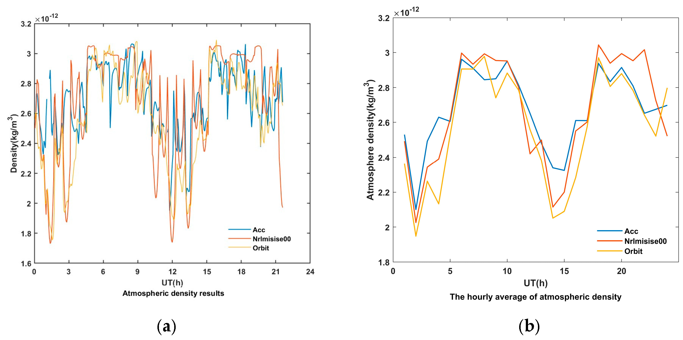
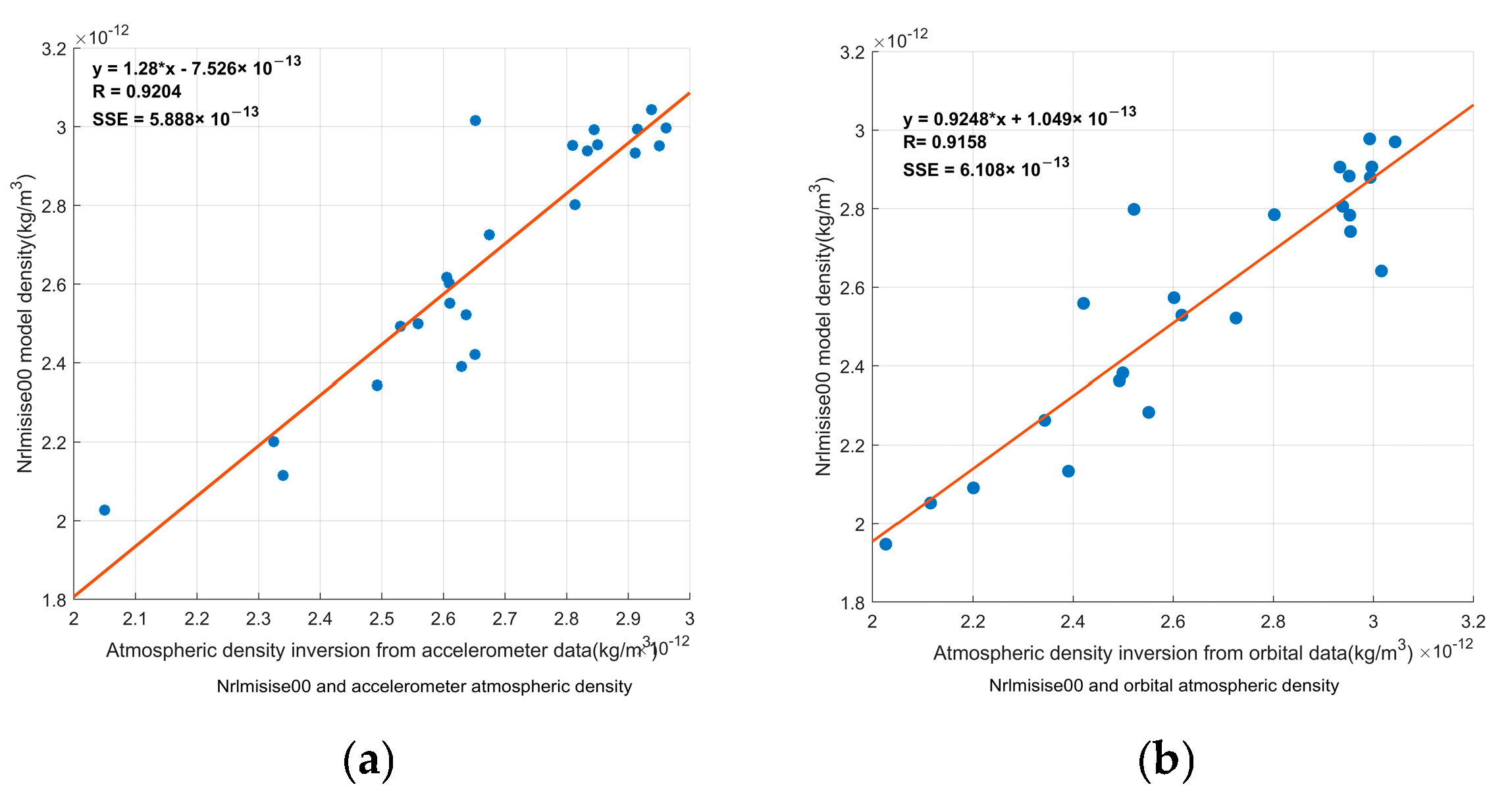
4.4. Inversion Results and Comparative Validation

The atmospheric density on 28 April 2024, can be calculated following Equation (5), contingent on the acquisition of the $C_D\ast A$ sum. Figure 4 illustrates the time-dependent atmospheric density obtained from the inversion. It can be observed that on 28 April 2024, the atmospheric density around the orbit of the SWARM-A satellite was approximately 10⁻¹² kg/m³. This cycle is closely related to the flight path of the SWARM-A satellite.

The inversion results were compared with the atmospheric density simulated by the Nrlmisise00 model. Based on the daily measured F10.7 and Ap indices provided by GFZ officials and their corresponding averages, combined with the geographic latitude and longitude positions obtained from precise orbit data, the data are input into the Nrlmisise00 model to obtain the corresponding atmospheric density. The time-averaged atmospheric density obtained through calculation was compared with the actual inversion results, and the analysis results are shown in Figure 5. From the graph, it can be seen that a review of the time series indicates that the atmospheric density of the two is highly consistent, and the overall trend of change is also similar. After linear fitting, the correlation coefficient between the accelerometer method and nrlmisise00 reached 0.9204, and the SSE was 5.888 × 10⁻¹³ in Figure 6a. The correlation coefficient between the semi-long axis attenuation method and nrlmisise00 reached 0.9158, and the SSE reached 6.108 × 10⁻¹³ in Figure 6b. The inversion accuracy of the accelerometer method was slightly higher than that of the semi-long axis attenuation method [53].

5. Conclusions

The composition and content of the atmosphere undergo significant alterations within the altitude range of Low Earth Orbit satellite operation as a consequence of the influence of various factors, including seasonal variations, solar activity, and geomagnetic indices. This results in the formation of the most active region of atmospheric drag. As the primary uptake force, it alters the operational velocity and attitude of the satellite. Atmospheric density inversion based on LEO satellites facilitates the adjustment of operational orbit altitude and velocity according to changes in atmospheric density, thereby prolonging operational cycles. Furthermore, the extensive observation data provided by LEO satellites can be fully utilized for atmospheric density modeling, which provides a reliable data source for weather numerical simulation and assimilation prediction.

This article presents an in-depth and objective comparative and critical analysis of the diverse methodologies utilized for the acquisition of atmospheric density data, the types of data required, and an evaluation of their respective advantages and disadvantages. The use of satellite-borne atmospheric density sounders allows for the coverage of a vast area of the Earth’s surface and the detection of phenomena at high altitudes. However, the costs associated with their launch and maintenance are considerable, and there may be delays in the processing and transmission of data, which limits the capability for real-time monitoring. The semi-axis decay method, which is based on dynamics, introduces an error associated with numerical integration and increases the computational volume when orbits are extrapolated. The energy decay method, which is based on the energy conservation theorem, greatly reduces the complexity of the calculation because it does not require the extrapolation of the orbit. There is an error in the energy form of some regenerative forces, which is particularly significant for orbits at higher altitudes. The acceleration calculated by the first two methods does not represent the actual instantaneous atmospheric drag acceleration; rather, it can be regarded as the average acceleration over the specified time interval. The accelerometer is capable of measuring the instantaneous acceleration with greater accuracy. The second part compares the precision orbit data and accelerometer data provided by the SWARM-A satellite. The semi-long axis attenuation method and accelerometer method were used for inversion experiments, and the inversion results were compared with the empirical model Nrlmisise00. The correlation coefficient between the semi-long axis attenuation method and Nrlmisise00 reached 0.9158, and the correlation coefficient between the accelerometer method and Nrlmisise00 reached 0.9204. The accuracy of accelerometer inversion is slightly higher than that of semi-long axis attenuation, which also confirms the feasibility of using orbit data for atmospheric density inversion and provides support for atmospheric modeling of LEO satellites without high-precision accelerometers.

References

1. McDowell, J.C. The edge of space: Revisiting the Karman Line. Acta Astronaut. 2018, 151, 668–677. [Google Scholar] [CrossRef]
2. Inter-Agency Space Debris Coordination Committee. IADC Space Debris Mitigation Guidelines; Central Research Institute of Machine Building: Koroylev, Russia, 2007; pp. 1–10. [Google Scholar]
3. Su, Y.; Liu, Y.; Zhou, Y.; Yuan, J.; Cao, H.; Shi, J. Broadband LEO satellite communications: Architectures and key technologies. IEEE Wirel. Commun. 2019, 26, 55–61. [Google Scholar] [CrossRef]
4. Horne, E.; Shafi, S.; Burke, J.; Prettitore, Z. SpaceX Report; Federal Aviation Administration: Washington, DC, USA. Available online: https://professordunagan.com/wp-content/uploads/2021/03/SpaceX-Report.pdf (accessed on 20 January 2025).
5. SpaceX 2019. Application for Fixed Satellite Service by Space Exploration Holdings. LLC, Technical Report, SAT-MOD-20190830-00087. Available online: https://fcc.report/IBFS/SAT-MOD-20190830-00087/1877764.pdf (accessed on 20 January 2025).
6. Henri, Y. The OneWeb satellite system. In Handbook of Small Satellites: Technology, Design, Manufacture, Applications, Economics and Regulation; Springer International Publishing: Berlin/Heidelberg, Germany, 2020; pp. 1091–1100. [Google Scholar]
7. Osoro, O.B.; Oughton, E.J.; Wilson, A.R.; Rao, A. Sustainability assessment of Low Earth Orbit (LEO) satellite broadband mega-constellations. arXiv 2023, arXiv:2309.02338. [Google Scholar]
8. Zhi, H.; Jiang, X.; Wang, J. Multicolour photometry of LEO mega-constellations Starlink and OneWeb. Mon. Not. R. Astron. Soc. 2024, 530, 5006–5015. [Google Scholar] [CrossRef]
9. Radtke, J.; Kebschull, C.; Stoll, E. Interactions of the space debris environment with mega constellations—Using the example of the OneWeb constellation. Acta Astronaut. 2017, 131, 55–68. [Google Scholar] [CrossRef]
10. Burns, A.G.; Solomon, S.C.; Qian, L.; Wang, W.; Emery, B.A.; Wiltberger, M.; Weimer, D.R. The effects of corotating interaction region/high speed stream storms on the thermosphere and ionosphere during the last solar minimum. J. Atmos. Sol.-Terr. Phys. 2012, 83, 79–87. [Google Scholar] [CrossRef]
11. Kavanagh, L.D., Jr.; Schardt, A.W.; Roelof, E.C. Solar wind and solar energetic particles: Properties and interactions. Rev. Geophys. 1970, 8, 389–460. [Google Scholar] [CrossRef]
12. Zhang, Y.; Bocquet, M.; Mallet, V.; Seigneur, C.; Baklanov, A. Real-time air quality forecasting, part II: State of the science, current research needs, and future prospects. Atmos. Environ. 2012, 60, 656–676. [Google Scholar] [CrossRef]
13. Yu, H.; Pang, Y.; Chen, B.; Feng, X.; Wang, B.; Zhao, Y. Simulation of orbital decay of LEO satellites due to atmospheric drag during magnetic storms. In Proceedings of the 2022 IEEE International Conference on Unmanned Systems (ICUS), Guangzhou, China, 28–30 October 2022; pp. 1179–1184. [Google Scholar] [CrossRef]
14. Calabia, A.; Jin, S.; Tenzer, R. A new GPS-based calibration of GRACE accelerometers using the arc-to-chord threshold uncovered sinusoidal disturbing signal. Aerosp. Sci. Technol. 2015, 45, 265–271. [Google Scholar] [CrossRef]
15. Calabia, A.; Jin, S. Thermospheric density estimation and responses to the March 2013 geomagnetic storm from GRACE GPS-determined precise orbits. J. Atmos. Sol.-Terr. Phys. 2017, 154, 167–179. [Google Scholar] [CrossRef]
16. Lundin, R.; Lammer, H.; Ribas, I. Planetary magnetic fields and solar forcing: Implications for atmospheric evolution. Space Sci. Rev. 2007, 129, 245–278. [Google Scholar] [CrossRef]
17. Champion KS, W.; Marcos, F.A. The triaxial—Accelerometer system on Atmosphere Explorer. Radio. Sci. 1973, 8, 297–303. [Google Scholar] [CrossRef]
18. Doornbos, E. Thermospheric Density and Wind Determination from Satellite Dynamics; Springer Science & Business Media: Berlin/Heidelberg, Germany, 2012. [Google Scholar]
19. March, G.; Visser, T.; Visser, P.; Doornbos, E.N. CHAMP and GOCE thermospheric wind characterization with improved gas-surface interactions modeling. Adv. Space Res. 2019, 64, 1225–1242. [Google Scholar] [CrossRef]
20. Tapley, B.D.; Bettadpur, S.; Watkins, M.; Reigber, C. The gravity recovery and climate experiment: Mission overview and early results. Geophys. Res. Lett. 2004, 31. [Google Scholar] [CrossRef]
21. Dang, T.; Lei, J.; Wang, W.; Zhang, B.; Burns, A.; Le, H.; Wu, Q.; Ruan, H.; Dou, X.; Wan, W. Global responses of the coupled thermosphere and ionosphere system to the August 2017 Great American Solar Eclipse. J. Geophys. Res. Space Phys. 2018, 123, 7040–7050. [Google Scholar] [CrossRef]
22. Lei, J.; Burns, A.G.; Thayer, J.P.; Wang, W.; Mlynczak, M.G.; Hunt, L.A.; Dou, X.; Sutton, E. Overcooling in the upper thermosphere during the recovery phase of the 2003 October storms. J. Geophys. Res. Space Phys. 2012, 117. [Google Scholar] [CrossRef]
23. Emmert, J.T. Thermospheric mass density: A review. Adv. Space Res. 2015, 56, 773–824. [Google Scholar] [CrossRef]
24. Celiberto, R.; Armenise, I.; Cacciatore, M.; Capitelli, M.; Esposito, F.; Gamallo, P.; Janev, R.K.; Laganà, A.; Laporta, V.; Laricchiuta, A. Atomic and molecular data for spacecraft re-entry plasmas. Plasma Sources Sci. Technol. 2016, 25, 033004. [Google Scholar] [CrossRef]
25. Van Leeuwen, P.J. Particle filtering in geophysical systems. Mon. Weather Rev. 2009, 137, 4089–4114. [Google Scholar] [CrossRef]
26. Sentman, L.H. Free Molecule Flow Theory and Its Application to the Determination of Aerodynamic Forces; Lockheed Missiles & Space Company: Sunnyvale, CA, USA, 1961. [Google Scholar]
27. Moe, K.; Moe, M.M. Gas–surface interactions and satellite drag coefficients. Planet. Space Sci. 2005, 53, 793–801. [Google Scholar] [CrossRef]
28. Vallado, D.A. Fundamentals of Astrodynamics and Applications; Springer Science & Business Media: Berlin/Heidelberg, Germany, 2001. [Google Scholar]
29. Curtis, H.D. Orbital Mechanics for Engineering Students: Revised Reprint; Butterworth-Heinemann: Oxford, UK, 2020. [Google Scholar]
30. Sang, J.; Smith, C.; Zhang, K. Towards accurate atmospheric mass density determination using precise positional information of space objects. Adv. Space Res. 2012, 49, 1088–1096. [Google Scholar] [CrossRef]
31. Gerlach, C.; Sneeuw, N.; Visser, P.; Švehla, D. CHAMP gravity field recovery using the energy balance approach. Adv. Geosci. 2003, 1, 73–80. [Google Scholar] [CrossRef]
32. Jekeli, C. The determination of gravitational potential differences from satellite-to-satellite tracking. Celest. Mech. Dyn. Astron. 1999, 75, 85–101. [Google Scholar] [CrossRef]
33. Pavlis, N.K.; Holmes, S.A.; Kenyon, S.C.; Factor, J.K. An earth gravitational model to degree 2160: EGm2008. In Proceedings of the 2008 General Assembly of the European Geosciences Union, Vienna, Austria, 13–18 April 2008. [Google Scholar]
34. Förste, C.; Schwintzer, P.; Reigber, C. Format Description: The CHAMP Data Format; CH-GFZ-FD-001; 2002. Available online: https://gfzpublic.gfz-potsdam.de/rest/items/item_18184_5/component/file_309987/content (accessed on 20 January 2025).
35. Miao, J.; Ren, T.; Gong, J.; Liu, S.; Li, Z. Atmospheric density inversion based on high-precision GPS observation data from satellites. J. Geophys. 2016, 59, 3566–3572. (In Chinese) [Google Scholar]
36. Li, R.X.; Lei, J.H.; Wang, X.J.; Dou, X.K.; Jin, S.G. Thermospheric mass density derived from CHAMP satellite precise orbit determination data based on energy balance method. Sci. China Earth Sci. 2017, 60, 1495–1506. [Google Scholar] [CrossRef]
37. Zhang, Z.; Zhang, Y.; Wang, B. Application of the hp-adaptive pseudospectral method in spacecraft orbit pursuit-evasion game. Adv. Space Res. 2024, 73, 1597–1610. [Google Scholar] [CrossRef]
38. Li, R.; Lei, J.; Wang, X.; Dou, X.; Jin, S. Using the energy attenuation method to invert the density of the thermosphere atmosphere using CHAMP satellite precise orbit data Chinese Science. Earth Sci. 2017, 47, 13. (In Chinese) [Google Scholar]
39. Bruinsma, S.; Tamagnan, D.; Biancale, R. Atmospheric densities derived from CHAMP/STAR accelerometer observations. Planet. Space Sci. 2004, 52, 297–312. [Google Scholar] [CrossRef]
40. Floberghagen, R.; Fehringer, M.; Lamarre, D.; Muzi, D.; Frommknecht, B.; Steiger, C.; da Costa, A. Mission design, operation, and exploitation of the gravity field and steady-state ocean circulation explorer mission. J. Geod. 2011, 85, 749–758. [Google Scholar] [CrossRef]
41. Livadiotti, S.; Crisp, N.H.; Roberts, P.C.E.; Worrall, S.D.; Oiko, V.T.A.; Edmondson, S.; Haigh, S.J.; Huyton, C.; Smith, K.L.; Sinpetru, L.A.; et al. A review of gas-surface interaction models for orbital aerodynamics applications. Prog. Aerosp. Sci. 2020, 119, 100675. [Google Scholar] [CrossRef]
42. Drinkwater, M.R.; Haagmans, R.; Muzi, D.; Muzi, D. The GOCE gravity mission: ESA’s first core Earth explorer. In Proceedings of the 3rd international GOCE user workshop, Noordwijk, Frascati, Italy, 6–8 November 2006; European Space Agency: Noordwijk, The Netherlands, 2006; pp. 6–8. [Google Scholar]
43. Reigber, C.; Lühr, H.; Schwintzer, P.; Wickert, J. Earth Observation with CHAMP. Results from Three Years; Springer: Berlin/Heidelberg, Germany, 2004. [Google Scholar]
44. van den IJssel, J.; Doornbos, E.; Iorfida, E.; March, G.; Siemes, C.; Montenbruck, O. Thermosphere densities derived from Swarm GPS observations. Adv. Space Res. 2020, 65, 1758–1771. [Google Scholar] [CrossRef]
45. Wickert, J.; Reigber, C.; Beyerle, G.; König, R.; Marquardt, C.; Schmidt, T.; Grunwaldt, L.; Galas, R.; Meehan, T.K.; Melbourne, W.G.; et al. Atmosphere sounding by GPS radio occultation: First results from CHAMP. Geophys. Res. Lett. 2001, 28, 3263–3266. [Google Scholar] [CrossRef]
46. Perosanz, F.; Biancale, R.; Lemoine, J.M.; Vales, N.; Loyer, S.; Bruinsma, S. Evaluation of the CHAMP Accelerometer on Two Years of Mission; Springer: Berlin/Heidelberg, Germany, 2005. [Google Scholar] [CrossRef]
47. Yin, L.; Wang, L.; Zheng, W.; Ge, L.; Tian, J.; Liu, Y.; Yang, B.; Liu, S. Evaluation of empirical atmospheric models using Swarm-C satellite data. Atmosphere 2022, 13, 294. [Google Scholar] [CrossRef]
48. Hajj, G.A.; Ao, C.O.; Iijima, B.A.; Kuang, D.; Kursinski, E.R.; Mannucci, A.J.; Meehan, T.K.; Romans, L.J.; de la Torre Juarez, M.; Yunck, T.P.; et al. CHAMP and SAC-C atmospheric occultation results and intercomparisons. J. Geophys. Res. Atmos. 2004, 109. [Google Scholar] [CrossRef]
49. Hwang, C.; Tseng, T.P.; Lin, T.; Schreiner, B. Precise orbit determination for the FORMOSAT-3/COSMIC satellite mission using GPS. J. Geod. 2009, 83, 477–489. [Google Scholar] [CrossRef]
50. Tang, G.; Li, X.; Cao, J.; Liu, S.; Chen, G.; Man, H.; Zhang, X.; Shi, S.; Sun, J.; Li, Y.; et al. APOD mission status and preliminary results. Sci. China Earth Sci. 2020, 63, 257–266. [Google Scholar] [CrossRef]
51. Kennedy, G.M.; Wyatt, M.C. Collisional evolution of irregular satellite swarms: Detectable dust around Solar system and extrasolar planets. Mon. Not. R. Astron. Soc. 2011, 412, 2137–2153. [Google Scholar] [CrossRef]
52. Michalak, A. Phenolic compounds and their antioxidant activity in plants growing under heavy metal stress. Pol. J. Environ. Stud. 2006, 15, 523–530. [Google Scholar]
53. Picone, J.M.; Hedin, A.E.; Drob, D.P.; Aikin, A.C. NRLMSISE-00 empirical model of the atmosphere: Statistical comparisons and scientific issues. J. Geophys. Res. Space Phys. 2002, 107, SIA 15-1–SIA 15-16. [Google Scholar] [CrossRef]
Figure 1. Search for articles using keywords “LEO Satellite” and “Low Earth Orbit Satellite” in the Web of Science database from 2015 to 2024 and keyword co-occurrence/clustering maps created using CiteSpace6.3.1 software in order to analyze research centered on LEO satellites and find the most important factors in the research of LEO satellites. In this figure, all words that co-occurred with LEO satellite keywords more than 50 times are displayed and automatically clustered according to the research field.
Remotesensing 17 00793 g001
Figure 2. Schematic diagram of inversion of orbit data and accelerometer data. The orbit data adopts the specific steps of semi-long-axis attenuation method and energy conservation method, and the accelerometer data are calibrated and inverted.
Remotesensing 17 00793 g002
Figure 3. The product of SWARM-A satellite damping factor and effective area is usually expressed by B, the anti-ballistic coefficient. The anti-ballistic coefficient of SWARM-A fluctuates between 2.56 and 2.58.
Remotesensing 17 00793 g003
Figure 4. On 28 April 2024, the atmospheric density inversion results of the SWARM-A satellite were obtained, with red indicating the semi-long axis attenuation method and blue indicating the accelerometer inversion. The atmospheric density varied from 1.6 to 3.2, and there was a minimum value at 15 UT (h) in the morning and noon.
Remotesensing 17 00793 g004
Figure 5. (a) On 28 April 2024, the atmospheric density inversion results were compared with the NRLMISISE00 model. Orange represents the Nrlmisise00 simulated density, green represents the semi-long axis attenuation method for atmospheric density inversion, and blue represents the accelerometer inversion. (b) We take the hourly average of atmospheric density on 28 April 2024. Blue represents the accelerometer average, green is the hourly average corresponding to the semi-long axis attenuation method, and orange is the hourly average density of the Nrlmisise00 model.
Remotesensing 17 00793 g005
Figure 6. We linearly fit the semi-long axis attenuation and velocity meter inversion results in Figure 5b with the empirical model, where (a) represents the fitting results of the accelerometer and nrlmisise00, and (b) represents the fitting effect of the semi-long axis attenuation and nrlmisise00.
Remotesensing 17 00793 g006