
An Improved Adaptive Multi-Scale Peak Detection Retracker for River Level Estimation Based on Sentinel-6 Fully Focused SAR Data


Abstract
1. Introduction
2. Materials and Methods
2.1. Study Area
2.2. Data
2.2.1. Altimeter Data and Processing
- Zero-padding the raw data in the along-track direction. The Sentinel-6 satellite operates in an interleaved mode with a dynamic pulse repetition frequency (PRF), so interpolation was employed to maintain a constant pulse repetition interval (PRI);
- Performing the Fourier transforms of the dataset in the along-track direction, one by one in the range direction;
- Along-track compression, including the multiplication of the transformed dataset by the focusing operator sample-by-sample;
- Complete focusing using double inverse Fourier transforms by applying the inverse Fast Fourier Transform (IFFT) algorithm to the azimuth and the Fast Fourier Transform (FFT) algorithm to the range direction;
- Compensating across the track.
2.2.2. Auxiliary Data
2.3. Methods
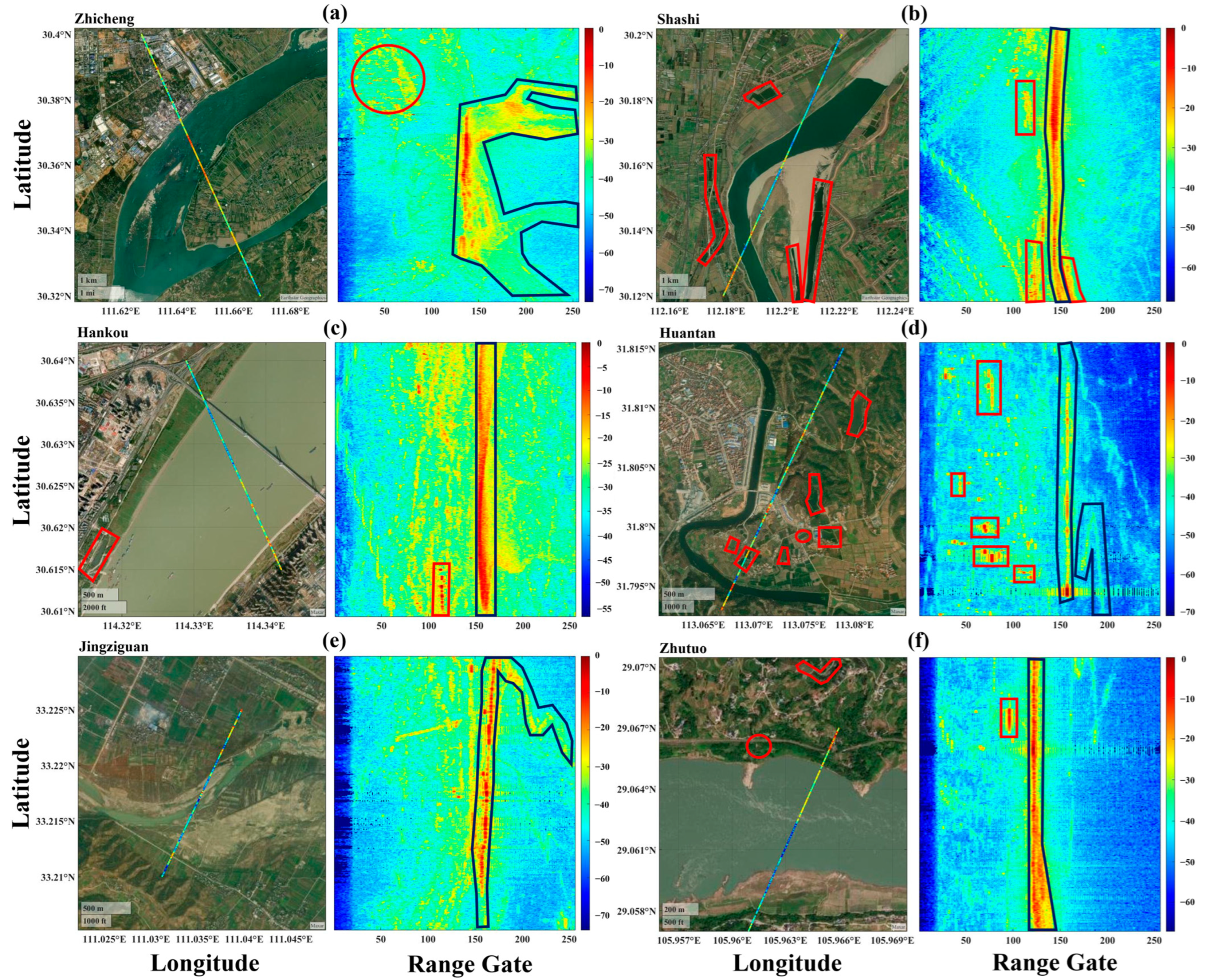
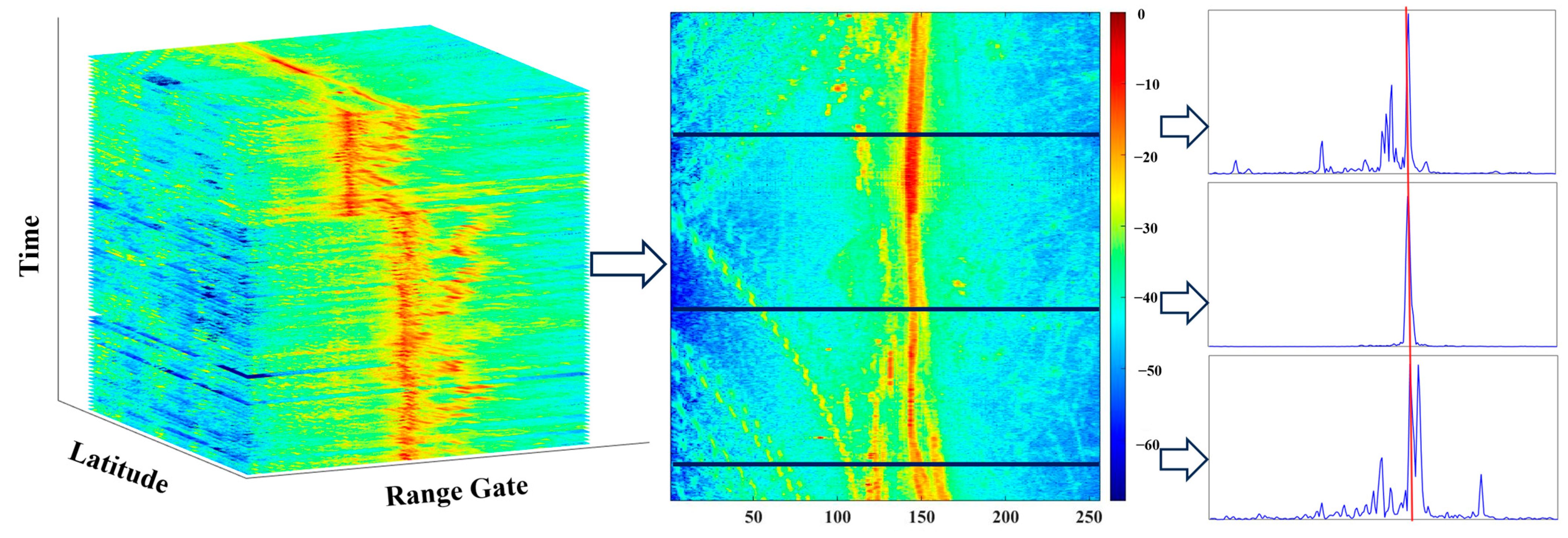
2.3.1. Analysis of River FF-SAR Waveform Features
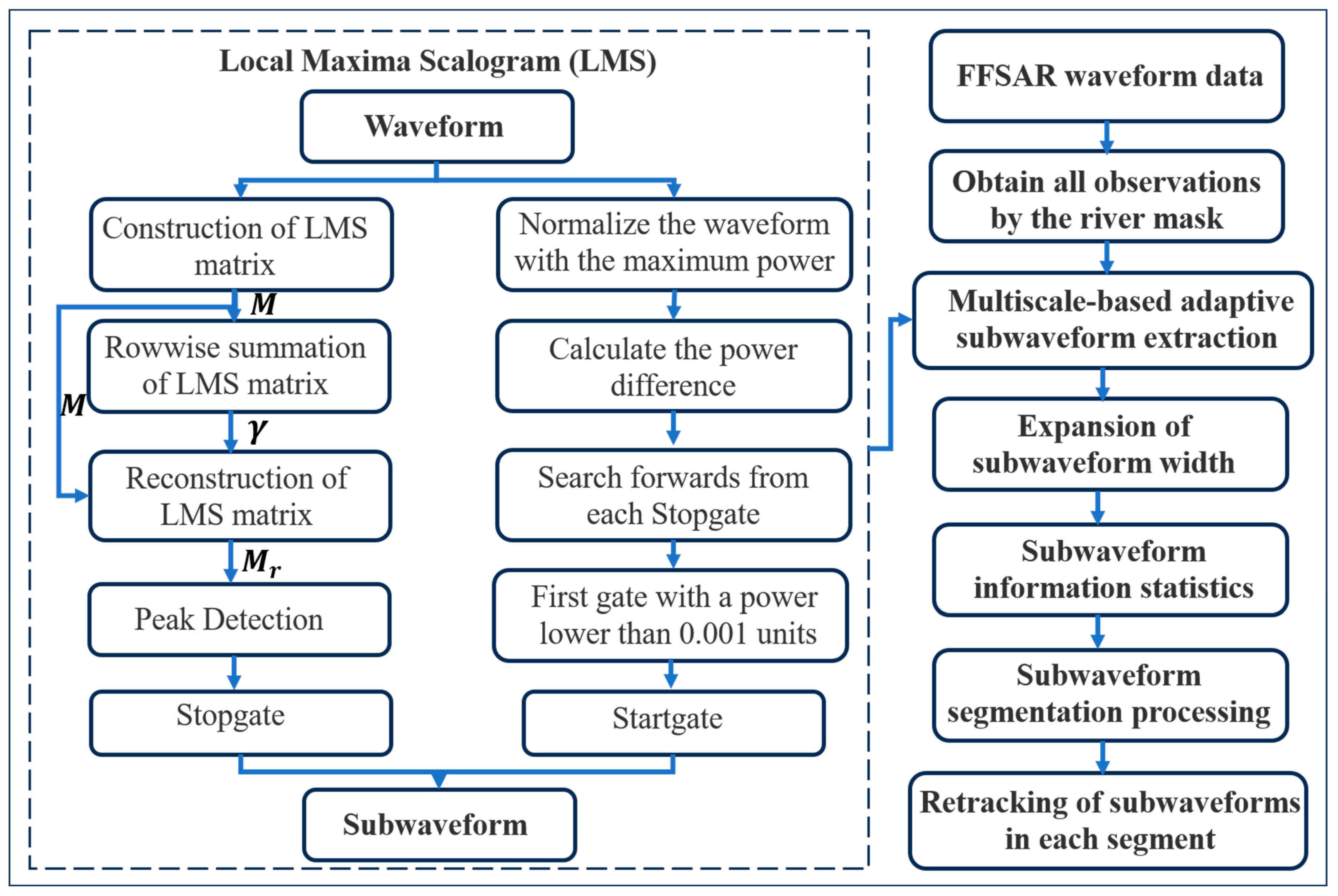
2.3.2. ImpAMPD Retracker
- To select daily overpass waveform data for the river segments in the study sections to obtain multiple waveform data;
- To extract multi-scale adaptive sub-wave peaks to accurately identify multiple strong sub-wave peak signals from each waveform based on the Local Maxima Scalogram (LMS) method [23] The key of this method is to construct an local maxima matrix for each waveform. The extraction process is as follows:Step 1: Calculate the local maxima of the waveform using a moving average window, where the window length varies according to . The local maxima for different window lengths : are determined by (1):where is a random number in the range [0, 1], is the -th waveform in the along-track direction, and is the power waveform. L = 5 is the optimal setting for peak detection in this study. The values of , at and are set to . Based on this, a local maxima matrix can be constructed.Step 2: Calculate the sum of each row of the local maxima matrix , denoted as .The row-wise summation contains information about the scale-dependent distribution of zeros (thus, local maxima). The global minimum of , denoted as , represents the dimension with the most local maxima. Additionally, use to reorganize the local maxima matrix LMS by removing all elements that satisfy , resulting in a new matrix .Step 3: To determine the peaks of the waveform by calculating the column-wise standard deviation of each column of the matrix according to (3).The index that satisfies represents the bins of the detected peak. This value is designated as the stopping point of the sub-waveform . For each waveform, can be determined.Additionally, to determine the starting point of each sub-waveform, the waveform is normalized with the maximum power. Subsequently, the power difference of the normalized waveform’s consecutive gates is calculated to obtain the power difference waveform. Finally, for each sub-waveform stopping point , the power difference waveform is searched from back to front. The first gate with a power value below 0.001 is identified as the corresponding sub-waveform starting point .Following the aforementioned steps, the same search is performed for all sub-waveform stopping points in , and ultimately, the sub-waveform starting points are calculated, forming N sub-waveforms together with . Considering that some situations may have sub-waveform widths of only 2–3 bins, which are too narrow for retracking calculations, it is necessary to extend several bins forward or backward to form new sub-waveforms. Previous studies have demonstrated that a sub-waveform width of at least five bins is optimal [24,25]. Therefore, the difference between the end and start gates is calculated to verify the sub-waveform length. For special sub-waveforms, two bins are extended either backward or forward;
- Sub-waveform information statistics. After the multi-scale adaptive sub-wave peak extraction, each row of the waveforms is traversed in the azimuth direction. Using the obtained start and end gates of each sub-waveform, the gate length of each sub-waveform is calculated and recorded in the array. The frequency of each gate length and its corresponding occurrence are then counted. Subsequently, the smallest gate length is selected from the top three most frequent gate lengths, denoted as the minimum gate length ;
- Sub-waveform segmentation. The number of segments in the waveforms is determined based on the number of gates.Each segment may contain multiple sub-wave peaks. To further remove interfering signals, the minimum gate length is halved, referred to as the narrow gate scheme, while the original gate length is referred to as the wide gate scheme. Each waveform is traversed to determine the segment of each sub-wave peak gate position. The top three segments with the most sub-wave peaks are identified, and the start and end gate positions and corresponding row numbers are recorded, denoted as ;
- Retracking of sub-waveform segments. Retracking is performed for each type of sub-waveform segment, and the corresponding height () is calculated. First, each sub-waveform is traversed to obtain its , , and . A temporary row (referred to as newRow) of the same size as a single waveform is created, with all values initialized to 0. The sub-waveform values are subsequently assigned to the corresponding gate positions in newRow. Thereafter, the PTR and Threshold retrackers are applied to the waveform in newRow. The Threshold is an extension of the OCOG retracker, defined as Threshold = thres·OCOG. The standard deviation and median of the heights for each sub-waveform segment are calculated, and heights exceeding three times the standard deviation from the median are removed. This outlier exclusion step is repeated three times. Finally, the water level () at several nadir points for the day is determined using the following formula [25],where is the satellite altitude, is the distance between the altimeter and the water surface, is the ionospheric correction, is the solid earth tide, is the wet troposphere, is the dry troposphere, and is the geoid height with respect to the ellipsoid, for which the 2008 Earth Gravitational Model (EGM2008) is used. Except for , all the above corrections are included in Sentinel-6 L2 products;
- Removing outliers for heights in the along-track direction. The heights for the same day are extracted based on the corresponding orbit number. The nearest neighbor linear interpolation method is employed to filter outliers. Subsequently, the average of the heights in the along-track direction is calculated and used as a baseline to exclude outliers beyond ±8 m;
- Slope correction and river level time series construction. Due to the slope of the river surface and the distance deviations of several nadir points during the observation period (see Figure 1), it is necessary to calculate the distance from each nadir point along the river centerline to the virtual station. Using the cumulative distance difference () and the slope (), the correction value to adjust the along-track water levels at the virtual station is calculated. The formula is given as follows:The median, mean, and standard deviation of the along-track water levels are then calculated. The standard deviation of along-track water levels is recorded as alStd.
2.3.3. Annual Change Rate of River Levels
3. Results
3.1. Sub-Waveform Segment Analysis
- The first segment has the highest number of sub-wave peaks, and the second and third segments have significantly lower numbers of sub-wave peaks than the first segment;
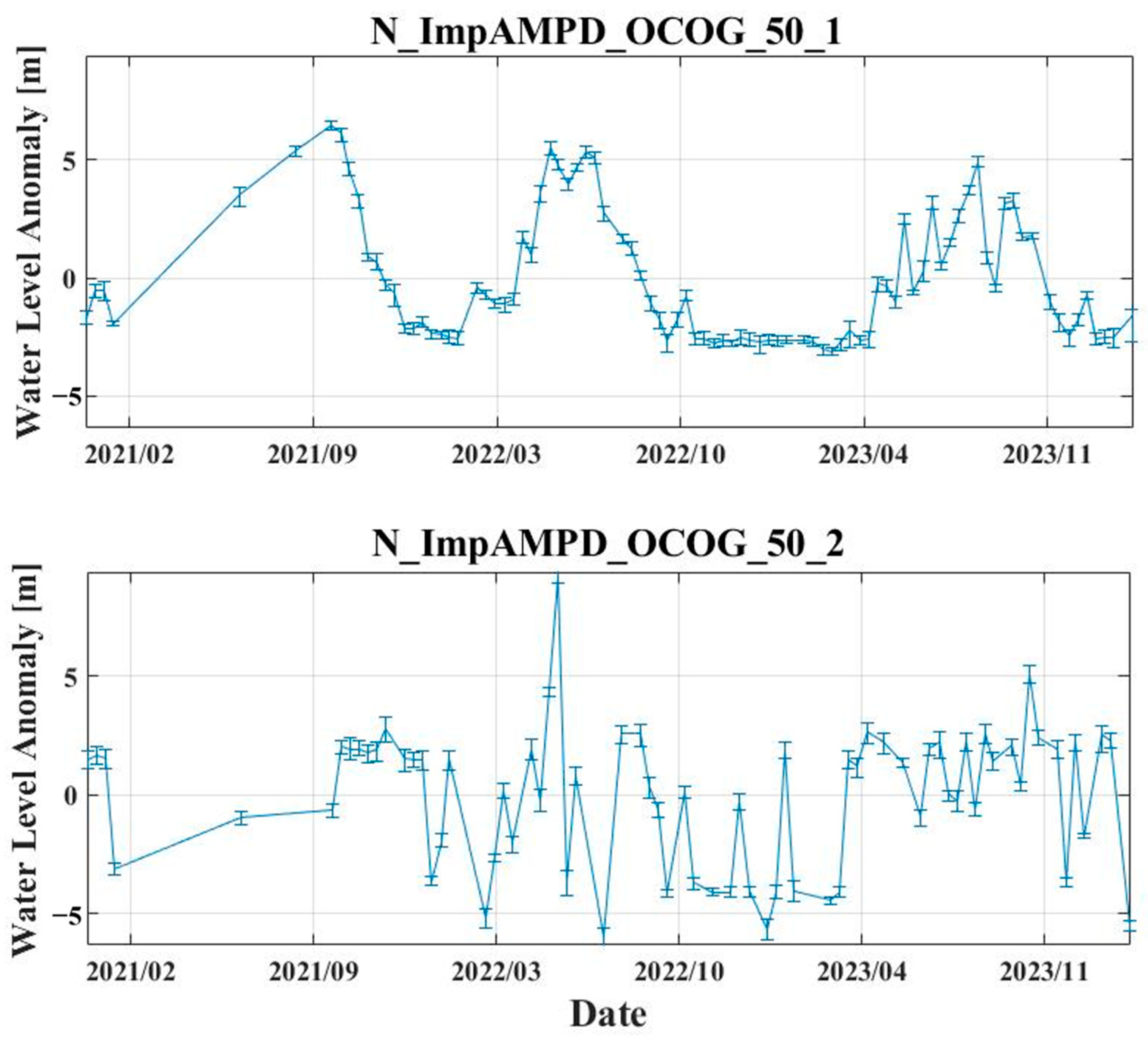
- Figure 5 and Figure 6 illustrate that the water level generated in the first segment is the most consistent with the in situ data, while the water level generated in the second segment has a low frequency of monitoring, a large range of elevation fluctuations, a high along-track standard deviation, and a large difference between the generated water level and in situ data;
- For the 1280 Hz_N_ImpAMPD waveform segment, the minimum gate length is 2. The first segment is mostly the 72nd–74th segments, which corresponds to the range of the dark blue box in Figure 2b, while the second segment is mostly the 62nd–66th segments, which corresponds to the range of the red box in Figure 2b, indicating that the sub-wave peaks in the second segment are the interfering signals from the non-river surfaces.
3.2. Accuracy Verification
3.2.1. Accuracy of the ImpAMPD Retracker
3.2.2. Comparative Analysis of Different Retrackers
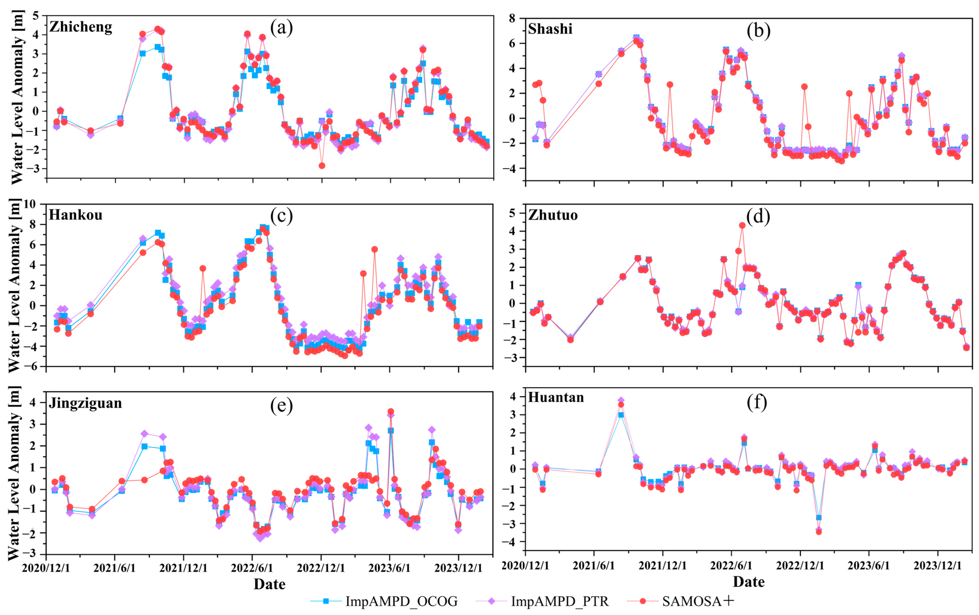
3.3. Water Level Time Series Analysis
3.3.1. Main Stream of the Yangtze River
3.3.2. Tributaries of the Yangtze River
4. Discussion
4.1. Performance of FF-SAR Data in River Level Estimation
4.2. Impact of Interfering Signals on Waveforms
4.3. Comparison of Retrackers’ Performance
4.3.1. The Existing Retrackers
4.3.2. The ImpAMPD Retracker
5. Conclusions
Author Contributions
Funding
Data Availability Statement
Acknowledgments
Conflicts of Interest
Appendix A

| Study Section | Posting Rate | Retracker | STDD (m) | CC 1 | No. | MalStd 2 (m) |
|---|---|---|---|---|---|---|
| Zhicheng | 1280 Hz | N_ImpAMPD_OCOG_40 | 0.47 | 0.96 | 75 | 0.091 |
| N_ImpAMPD_OCOG_45 | 0.55 | 0.93 | 75 | 0.102 | ||
| N_ImpAMPD_OCOG_50 | 0.55 | 0.93 | 75 | 0.114 | ||
| N_ImpAMPD_PTR | 0.47 | 0.95 | 75 | 0.056 | ||
| W_ImpAMPD_OCOG_40 | 0.89 | 0.79 | 72 | 0.155 | ||
| W_ImpAMPD_OCOG_45 | 0.89 | 0.78 | 72 | 0.174 | ||
| W_ImpAMPD_OCOG_50 | 0.90 | 0.78 | 72 | 0.192 | ||
| W_ImpAMPD_PTR | 0.96 | 0.75 | 72 | 0.176 | ||
| OCOG | 0.66 | 0.91 | 76 | 0.543 | ||
| PTR | 0.66 | 0.90 | 76 | 0.685 | ||
| SAMOSA+ | 0.58 | 0.93 | 76 | 0.527 | ||
| 640 Hz | N_ImpAMPD_OCOG_40 | 0.48 | 0.96 | 75 | 0.087 | |
| N_ImpAMPD_OCOG_45 | 0.48 | 0.96 | 75 | 0.098 | ||
| N_ImpAMPD_OCOG_50 | 0.48 | 0.96 | 75 | 0.109 | ||
| N_ImpAMPD_PTR | 0.56 | 0.93 | 75 | 0.047 | ||
| W_ImpAMPD_OCOG_40 | 0.85 | 0.83 | 72 | 0.142 | ||
| W_ImpAMPD_OCOG_45 | 0.84 | 0.81 | 71 | 0.159 | ||
| W_ImpAMPD_OCOG_50 | 0.84 | 0.80 | 71 | 0.175 | ||
| W_ImpAMPD_PTR | 0.839 | 0.803 | 71 | 0.159 | ||
| OCOG | 0.58 | 0.93 | 76 | 0.356 | ||
| PTR | 0.58 | 0.93 | 76 | 0.493 | ||
| SAMOSA+ | 0.53 | 0.94 | 76 | 0.352 | ||
| 160 Hz | N_ImpAMPD_OCOG_40 | 0.51 | 0.95 | 74 | 0.082 | |
| N_ImpAMPD_OCOG_45 | 0.50 | 0.95 | 74 | 0.092 | ||
| N_ImpAMPD_OCOG_50 | 0.50 | 0.95 | 74 | 0.103 | ||
| N_ImpAMPD_PTR | 0.51 | 0.95 | 74 | 0.044 | ||
| W_ImpAMPD_OCOG_40 | 0.71 | 0.87 | 71 | 0.130 | ||
| W_ImpAMPD_OCOG_45 | 0.73 | 0.87 | 71 | 0.146 | ||
| W_ImpAMPD_OCOG_50 | 0.73 | 0.87 | 71 | 0.163 | ||
| W_ImpAMPD_PTR | 0.75 | 0.86 | 71 | 0.134 | ||
| OCOG | 0.55 | 0.93 | 76 | 0.299 | ||
| PTR | 0.55 | 0.93 | 76 | 0.312 | ||
| SAMOSA+ | 0.53 | 0.94 | 76 | 0.311 | ||
| Shashi | 1280 Hz | N_ImpAMPD_OCOG_40 | 1.52 | 0.89 | 68 | 0.085 |
| N_ImpAMPD_OCOG_45 | 0.70 | 0.98 | 68 | 0.095 | ||
| N_ImpAMPD_OCOG_50 | 0.26 | 1.00 | 68 | 0.106 | ||
| N_ImpAMPD_PTR | 0.27 | 1.00 | 68 | 0.031 | ||
| W_ImpAMPD_OCOG_40 | 1.51 | 0.82 | 63 | 0.113 | ||
| W_ImpAMPD_OCOG_45 | 1.21 | 0.92 | 63 | 0.127 | ||
| W_ImpAMPD_OCOG_50 | 1.08 | 0.92 | 63 | 0.141 | ||
| W_ImpAMPD_PTR | 1.08 | 0.92 | 63 | 0.112 | ||
| OCOG | 1.81 | 0.75 | 71 | 0806 | ||
| PTR | 1.37 | 0.86 | 71 | 0.762 | ||
| SAMOSA+ | 1.50 | 0.84 | 71 | 0.947 | ||
| 640 Hz | N_ImpAMPD_OCOG_40 | 1.52 | 0.89 | 67 | 0.078 | |
| N_ImpAMPD_OCOG_45 | 0.70 | 0.98 | 67 | 0.087 | ||
| N_ImpAMPD_OCOG_50 | 0.27 | 1.00 | 67 | 0.097 | ||
| N_ImpAMPD_PTR | 0.28 | 1.00 | 67 | 0.021 | ||
| W_ImpAMPD_OCOG_40 | 1.46 | 0.84 | 64 | 0.108 | ||
| W_ImpAMPD_OCOG_45 | 1.18 | 0.90 | 64 | 0.122 | ||
| W_ImpAMPD_OCOG_50 | 1.08 | 0.92 | 64 | 0.135 | ||
| W_ImpAMPD_PTR | 1.10 | 0.92 | 64 | 0.106 | ||
| OCOG | 1.79 | 0.76 | 71 | 1.233 | ||
| PTR | 1.26 | 0.88 | 71 | 0.618 | ||
| SAMOSA+ | 1.41 | 0.86 | 71 | 0.640 | ||
| 160 Hz | N_ImpAMPD_OCOG_40 | 1.24 | 0.92 | 62 | 0.069 | |
| N_ImpAMPD_OCOG_45 | 0.60 | 0.98 | 62 | 0.077 | ||
| N_ImpAMPD_OCOG_50 | 0.28 | 1.00 | 62 | 0.086 | ||
| N_ImpAMPD_PTR | 0.29 | 1.00 | 62 | 0.020 | ||
| W_ImpAMPD_OCOG_40 | 1.77 | 0.75 | 63 | 0.105 | ||
| W_ImpAMPD_OCOG_45 | 1.59 | 0.81 | 63 | 0.118 | ||
| W_ImpAMPD_OCOG_50 | 1.56 | 0.83 | 63 | 0.131 | ||
| W_ImpAMPD_PTR | 1.59 | 0.82 | 63 | 0.092 | ||
| OCOG | 1.87 | 0.73 | 71 | 0.639 | ||
| PTR | 1.29 | 0.88 | 71 | 0.545 | ||
| SAMOSA+ | 1.02 | 0.93 | 71 | 0.325 | ||
| Hankou | 1280 Hz | N_ImpAMPD_OCOG_40 | 1.12 | 0.95 | 71 | 0.081 |
| N_ImpAMPD_OCOG_45 | 0.57 | 0.99 | 71 | 0.091 | ||
| N_ImpAMPD_OCOG_50 | 0.18 | 1.00 | 70 | 0.099 | ||
| N_ImpAMPD_PTR | 0.21 | 1.00 | 59 | 0.064 | ||
| W_ImpAMPD_OCOG_40 | 3.00 | 0.59 | 66 | 0.122 | ||
| W_ImpAMPD_OCOG_45 | 2.96 | 0.62 | 65 | 0.132 | ||
| W_ImpAMPD_OCOG_50 | 2.85 | 0.66 | 64 | 0.141 | ||
| W_ImpAMPD_PTR | 3.19 | 0.57 | 61 | 0.110 | ||
| OCOG | 5.00 | −0.06 | 73 | 1.831 | ||
| PTR | 2.56 | 0.69 | 76 | 1.584 | ||
| SAMOSA+ | 1.58 | 0.90 | 75 | 1.372 | ||
| 640 Hz | N_ImpAMPD_OCOG_40 | 1.19 | 0.94 | 71 | 0.075 | |
| N_ImpAMPD_OCOG_45 | 0.67 | 0.98 | 71 | 0.084 | ||
| N_ImpAMPD_OCOG_50 | 0.35 | 0.99 | 70 | 0.093 | ||
| N_ImpAMPD_PTR | 0.58 | 0.98 | 62 | 0.036 | ||
| W_ImpAMPD_OCOG_40 | 2.26 | 0.73 | 65 | 0.102 | ||
| W_ImpAMPD_OCOG_45 | 2.09 | 0.77 | 65 | 0.114 | ||
| W_ImpAMPD_OCOG_50 | 2.02 | 0.78 | 65 | 0.125 | ||
| W_ImpAMPD_PTR | 2.10 | 0.75 | 61 | 0.099 | ||
| OCOG | 5.37 | −0.18 | 71 | 1.714 | ||
| PTR | 2.55 | 0.70 | 76 | 1.428 | ||
| SAMOSA+ | 1.64 | 0.88 | 76 | 0.810 | ||
| 160 Hz | N_ImpAMPD_OCOG_40 | 1.99 | 0.82 | 71 | 0.070 | |
| N_ImpAMPD_OCOG_45 | 1.83 | 0.85 | 71 | 0.078 | ||
| N_ImpAMPD_OCOG_50 | 1.28 | 0.93 | 70 | 0.085 | ||
| N_ImpAMPD_PTR | 1.41 | 0.90 | 58 | 0.032 | ||
| W_ImpAMPD_OCOG_40 | 3.09 | 0.54 | 67 | 0.097 | ||
| W_ImpAMPD_OCOG_45 | 2.36 | 0.71 | 65 | 0.109 | ||
| W_ImpAMPD_OCOG_50 | 2.39 | 0.71 | 65 | 0.118 | ||
| W_ImpAMPD_PTR | 2.47 | 0.67 | 60 | 0.073 | ||
| OCOG | 5.17 | −0.05 | 70 | 1.551 | ||
| PTR | 3.11 | 0.57 | 76 | 1.349 | ||
| SAMOSA+ | 1.52 | 0.90 | 76 | 0.264 | ||
| Zhutuo | 1280 Hz | N_ImpAMPD_OCOG_40 | 0.41 | 0.99 | 18 | 0.046 |
| N_ImpAMPD_OCOG_45 | 0.35 | 0.99 | 18 | 0.052 | ||
| N_ImpAMPD_OCOG_50 | 0.33 | 0.99 | 18 | 0.058 | ||
| N_ImpAMPD_PTR | 0.34 | 0.99 | 18 | 0.014 | ||
| W_ImpAMPD_OCOG_40 | 1.28 | 0.43 | 18 | 0.063 | ||
| W_ImpAMPD_OCOG_45 | 1.32 | 0.43 | 18 | 0.071 | ||
| W_ImpAMPD_OCOG_50 | 1.39 | 0.45 | 18 | 0.079 | ||
| W_ImpAMPD_PTR | 1.41 | 0.44 | 18 | 0.050 | ||
| OCOG | 0.30 | 0.99 | 18 | 0.073 | ||
| PTR | 0.31 | 0.99 | 18 | 0.093 | ||
| SAMOSA+ | 0.30 | 0.99 | 18 | 0.073 | ||
| 640 Hz | N_ImpAMPD_OCOG_40 | 0.45 | 0.98 | 18 | 0.041 | |
| N_ImpAMPD_OCOG_45 | 0.42 | 0.98 | 18 | 0.046 | ||
| N_ImpAMPD_OCOG_50 | 0.44 | 0.98 | 18 | 0.051 | ||
| N_ImpAMPD_PTR | 0.44 | 0.98 | 18 | 0.011 | ||
| W_ImpAMPD_OCOG_40 | 1.26 | 0.44 | 18 | 0.059 | ||
| W_ImpAMPD_OCOG_45 | 1.30 | 0.44 | 18 | 0.067 | ||
| W_ImpAMPD_OCOG_50 | 1.36 | 0.44 | 18 | 0.074 | ||
| W_ImpAMPD_PTR | 1.39 | 0.42 | 18 | 0.047 | ||
| OCOG | 0.30 | 0.99 | 18 | 0.057 | ||
| PTR | 0.30 | 0.99 | 18 | 0.077 | ||
| SAMOSA+ | 0.30 | 0.99 | 18 | 0.064 | ||
| 160 Hz | N_ImpAMPD_OCOG_40 | 0.40 | 0.97 | 17 | 0.041 | |
| N_ImpAMPD_OCOG_45 | 0.34 | 0.97 | 17 | 0.046 | ||
| N_ImpAMPD_OCOG_50 | 0.34 | 0.97 | 17 | 0.051 | ||
| N_ImpAMPD_PTR | 0.54 | 0.91 | 17 | 0.011 | ||
| W_ImpAMPD_OCOG_40 | 1.26 | 0.46 | 18 | 0.074 | ||
| W_ImpAMPD_OCOG_45 | 1.30 | 0.46 | 18 | 0.083 | ||
| W_ImpAMPD_OCOG_50 | 1.37 | 0.46 | 18 | 0.092 | ||
| W_ImpAMPD_PTR | 1.41 | 0.44 | 18 | 0.011 | ||
| OCOG | 0.30 | 0.99 | 18 | 0.058 | ||
| PTR | 0.31 | 0.99 | 18 | 0.077 | ||
| SAMOSA+ | 0.30 | 0.99 | 18 | 0.064 | ||
| Jingziguan | 1280 Hz | N_ImpAMPD_OCOG_40 | 1.32 | 0.46 | 17 | 0.050 |
| N_ImpAMPD_OCOG_45 | 1.49 | 0.46 | 17 | 0.056 | ||
| N_ImpAMPD_OCOG_50 | 1.69 | 0.46 | 17 | 0.062 | ||
| N_ImpAMPD_PTR | 1.61 | 0.46 | 17 | 0.155 | ||
| W_ImpAMPD_OCOG_40 | 0.86 | 0.68 | 16 | 0.073 | ||
| W_ImpAMPD_OCOG_45 | 1.02 | 0.68 | 16 | 0.083 | ||
| W_ImpAMPD_OCOG_50 | 1.15 | 0.68 | 16 | 0.093 | ||
| W_ImpAMPD_PTR | 0.83 | 0.83 | 16 | 0.060 | ||
| OCOG | 0.73 | 0.45 | 17 | 0.134 | ||
| PTR | 0.77 | 0.45 | 17 | 0.088 | ||
| SAMOSA+ | 0.79 | 0.46 | 17 | 0.079 | ||
| 640 Hz | N_ImpAMPD_OCOG_40 | 0.97 | 0.52 | 15 | 0.042 | |
| N_ImpAMPD_OCOG_45 | 1.10 | 0.52 | 15 | 0.047 | ||
| N_ImpAMPD_OCOG_50 | 1.23 | 0.52 | 15 | 0.052 | ||
| N_ImpAMPD_PTR | 1.14 | 0.54 | 15 | 0.019 | ||
| W_ImpAMPD_OCOG_40 | 1.70 | −0.15 | 17 | 0.081 | ||
| W_ImpAMPD_OCOG_45 | 1.88 | −0.15 | 17 | 0.093 | ||
| W_ImpAMPD_OCOG_50 | 2.06 | −0.15 | 17 | 0.103 | ||
| W_ImpAMPD_PTR | 2.01 | −0.15 | 17 | 0.068 | ||
| OCOG | 0.73 | 0.47 | 17 | 0.125 | ||
| PTR | 0.85 | 0.32 | 17 | 0.076 | ||
| SAMOSA+ | 0.79 | 0.45 | 17 | 0.064 | ||
| 160 Hz | OCOG | 0.74 | 0.38 | 17 | 0.082 | |
| PTR | 0.79 | 0.35 | 17 | 0.090 | ||
| SAMOSA+ | 0.79 | 0.35 | 17 | 0.054 | ||
| Huantan | 1280 Hz | N_ImpAMPD_OCOG_40 | 0.60 | 0.42 | 67 | 0.015 |
| N_ImpAMPD_OCOG_45 | 0.65 | 0.42 | 67 | 0.017 | ||
| N_ImpAMPD_OCOG_50 | 0.71 | 0.52 | 67 | 0.018 | ||
| N_ImpAMPD_PTR | 0.72 | 0.42 | 68 | 0.001 | ||
| W_ImpAMPD_OCOG_40 | 0.53 | 0.46 | 69 | 0.022 | ||
| W_ImpAMPD_OCOG_45 | 0.58 | 0.46 | 69 | 0.025 | ||
| W_ImpAMPD_OCOG_50 | 0.63 | 0.46 | 69 | 0.028 | ||
| W_ImpAMPD_PTR | 0.53 | 0.47 | 69 | 0.001 | ||
| OCOG | 0.61 | 0.35 | 69 | 0.040 | ||
| PTR | 0.71 | 0.46 | 69 | 0.050 | ||
| SAMOSA+ | 0.39 | 0.35 | 69 | 0.020 | ||
| 640 Hz | N_ImpAMPD_OCOG_40 | 0.67 | 0.40 | 65 | 0.009 | |
| N_ImpAMPD_OCOG_45 | 0.74 | 0.40 | 65 | 0.011 | ||
| N_ImpAMPD_OCOG_50 | 0.81 | 0.40 | 65 | 0.012 | ||
| N_ImpAMPD_PTR | 0.82 | 0.430 | 65 | 0.003 | ||
| W_ImpAMPD_OCOG_40 | 0.36 | 0.41 | 67 | 0.020 | ||
| W_ImpAMPD_OCOG_45 | 0.37 | 0.42 | 67 | 0.022 | ||
| W_ImpAMPD_OCOG_50 | 0.38 | 0.42 | 67 | 0.020 | ||
| W_ImpAMPD_PTR | 0.39 | 0.47 | 68 | 0.013 | ||
| OCOG | 0.56 | 0.37 | 68 | 0.050 | ||
| PTR | 0.73 | 0.40 | 66 | 0.013 | ||
| SAMOSA+ | 0.38 | 0.31 | 69 | 0.015 | ||
| 160 Hz | OCOG | 0.56 | 0.39 | 68 | 0.145 | |
| PTR | 0.69 | 0.40 | 68 | 0.103 | ||
| SAMOSA+ | 0.37 | 0.36 | 69 | 0.012 |
References
- Vignudelli, S.; Scozzari, A.; Abileah, R.; Gómez-Enri, J.; Benveniste, J.; Cipollini, P. Chapter Four—Water surface elevation in coastal and inland waters using satellite radar altimetry. In Extreme Hydroclimatic Events and Multivariate Hazards in a Changing Environment; Maggioni, V., Massari, C., Eds.; Elsevier: Amsterdam, The Netherlands, 2019; pp. 87–127. [Google Scholar]
- Bašić, T. (Ed.) Satellite Altimetry—Theory, Applications and Recent Advances; IntechOpen: London, UK, 2023. [Google Scholar]
- Raney, R.K. The delay/Doppler radar altimeter. IEEE Trans. Geosci. Remote Sens. 1998, 36, 1578–1588. [Google Scholar] [CrossRef]
- Raney, R.K. CryoSat SAR-Mode Looks Revisited. IEEE Geosci. Remote Sens. Lett. 2012, 9, 393–397. [Google Scholar] [CrossRef]
- Wingham, D.J.; Phalippou, L.; Mavrocordatos, C.; Wallis, D. The mean echo and echo cross product from a beamforming interferometric altimeter and their application to elevation measurement. IEEE Trans. Geosci. Remote Sens. 2004, 42, 2305–2323. [Google Scholar] [CrossRef]
- Hernández-Burgos, S.; Gibert, F.; Broquetas, A.; Kleinherenbrink, M.; Cruz, A.F.D.l.; Gómez-Olivé, A. A Fully Focused SAR Omega-K Closed-Form Algorithm for the Sentinel-6 Radar Altimeter: Methodology and Applications. IEEE Trans. Geosci. Remote Sens. 2024, 62, 1–16. [Google Scholar] [CrossRef]
- Donlon, C.; Cullen, R.; Giulicchi, L.; Fornari, M.; Vuilleumier, P. Copernicus Sentinel-6 Michael Freilich Satellite Mission: Overview and Preliminary in Orbit Results. In Proceedings of the IEEE International Geoscience and Remote Sensing Symposium IGARSS, Brussels, Belgium, 11–16 July 2021; pp. 7732–7735. [Google Scholar]
- Amraoui, S.; Moreau, T. FFSAR replica removal algorithm for closed-burst data, Collecte Localisation Satellites (CLS). Tech. Rep. 2022. [Google Scholar] [CrossRef]
- Egido, A.; Smith, W.H.F. Fully Focused SAR Altimetry: Theory and Applications. IEEE Trans. Geosci. Remote Sens. 2017, 55, 392–406. [Google Scholar] [CrossRef]
- Guccione, P.; Scagliola, M.; Giudici, D. 2D Frequency Domain Fully Focused SAR Processing for High PRF Radar Altimeters. Remote Sens. 2018, 10, 1943. [Google Scholar] [CrossRef]
- Kleinherenbrink, M.; Naeije, M.; Slobbe, C.; Egido, A.; Smith, W. The performance of CryoSat-2 fully-focussed SAR for inland water-level estimation. Remote Sens. Environ. 2020, 237, 111589. [Google Scholar] [CrossRef]
- Feng, H.; Egido, A.; Vandemark, D.; Wilkin, J. Exploring the potential of Sentinel-3 delay Doppler altimetry for enhanced detection of coastal currents along the Northwest Atlantic shelf. Adv. Space Res. 2023, 71, 997–1016. [Google Scholar] [CrossRef]
- Schlembach, F.; Ehlers, F.; Kleinherenbrink, M.; Passaro, M.; Dettmering, D.; Seitz, F. Benefits of fully focused SAR altimetry to coastal wave height estimates: A case study in the North Sea. Remote Sens. Environ. 2023, 289, 113517. [Google Scholar] [CrossRef]
- Ehlers, F.; Schlembach, F.; Kleinherenbrink, M.; Slobbe, C. Validity assessment of SAMOSA retracking for fully-focused SAR altimeter waveforms. Adv. Space Res. 2023, 71, 1377–1396. [Google Scholar] [CrossRef]
- Wingham, D.; Rapley, C.; Griffiths, H. New techniques in satellite altimeter tracking systems. In Proceedings of the International Geoscience and Remote Sensing Symposium IGARSS, Zürich, Switzerland, 8–11 September 1986; pp. 1339–1344. [Google Scholar]
- Buchhaupt, C.; Fenoglio-Marc, L.; Dinardo, S.; Scharroo, R.; Becker, M. A fast convolution based waveform model for conventional and unfocused SAR altimetry. Adv. Space Res. 2018, 62, 1445–1463. [Google Scholar] [CrossRef]
- Dinardo, S.; Fenoglio-Marc, L.; Buchhaupt, C.; Becker, M.; Scharroo, R.; Joana, F.M. Coastal SAR and PLRM altimetry in German Bight and West Baltic Sea. Adv. Space Res. 2018, 62, 1371–1404. [Google Scholar] [CrossRef]
- Chen, J.; Liu, X.; Chen, J.; Jin, H.; Wang, T.; Zhu, W.; Li, L. Underestimated nutrient from aquaculture ponds to Lake Eutrophication: A case study on Taihu Lake Basin. J. Hydrol. 2024, 630, 130749. [Google Scholar] [CrossRef]
- Scharroo, R.; Bonekamp, H.; Ponsard, C.; Parisot, F.; von Engeln, A.; Tahtadjiev, M.; de Vriendt, K.; Montagner, F. Jason continuity of services: Continuing the Jason altimeter data records as Copernicus Sentinel-6. Ocean Sci. 2016, 12, 471–479. [Google Scholar] [CrossRef]
- Carrara, W.G.; Goodman, R.S.; Majewski, R.M. Spotlight Synthetic Aperture Radar: Signal Processing Algorithms; Artech House: Norwood, MA, USA, 1995. [Google Scholar]
- Chen, J.; Fenoglio, L.; Kusche, J. Measuring Off-nadir river water levels and slopes from altimeter Fully-Focused SAR mode. J. Hydrol. 2025, 650, 132553. [Google Scholar] [CrossRef]
- Papoulis, A. Systems and Transforms with Applications in Optics; R. Krieger Publishing Company: Malabar, FL, USA, 1968; ISBN 100070484570. [Google Scholar]
- Scholkmann, F.; Boss, J.; Wolf, M. An Efficient Algorithm for Automatic Peak Detection in Noisy Periodic and Quasi-Periodic Signals. Algorithms 2012, 5, 588–603. [Google Scholar] [CrossRef]
- Passaro, M.; Rose, S.K.; Andersen, O.B.; Boergens, E.; Calafat, F.M.; Dettmering, D. ALES plus: Adapting a homogenous ocean retracker for satellite altimetry to sea ice leads, coastal and inland waters. Remote Sens. Environ. 2018, 211, 456–471. [Google Scholar] [CrossRef]
- Chen, J.; Liao, J.; Wang, C. Improved Lake Level Estimation From Radar Altimeter Using an Automatic Multiscale-Based Peak Detection Retracker. IEEE J. Sel. Top. Appl. Earth Obs. Remote Sens. 2021, 14, 1246–1259. [Google Scholar] [CrossRef]
- Gao, L.; Liao, J.J.; Shen, G.Z. Monitoring lake-level changes in the Qinghai-Tibetan Plateau using radar altimeter data (2002–2012). J. Appl. Remote Sens. 2013, 7, 073470. [Google Scholar] [CrossRef]
- Tourian, M.J.; Elmi, O.; Khalili, S.; Engels, J. Improving Inland Water Altimetry Through Bin-Space-Time (BiST) Retracking: A Bayesian Approach to Incorporate Spatiotemporal Information. IEEE Trans. Geosci. Remote Sens. 2025, 63, 1–19. [Google Scholar] [CrossRef]


| Study Section | Duration 1 | Coordinates 2 (N, E) | Width (m) | Landscape 3 | Slope 4 (m/km) | Mode 5 |
|---|---|---|---|---|---|---|
| Zhicheng | 8 January 2022–11 February 2024 | 30.30, 111.50 | (1800, 2000) | Sandbar, Pond | 0.201 | Relative |
| Shashi | 8 January 2022–10 February 2024 | 30.31, 112.23 | (600, 1600) | Sandbank, Pond | 0.096 | Relative |
| Hankou | 1 January 2022–25 January 2024 | 30.56, 114.29 | (1400, 2000) | Bridge, Pond, Ships | 0.031 | Relative |
| Zhutuo | 31 December 2020–23 December 2021 | 29.01, 105.85 | (300, 500) | Shoal, Pond | 0.929 | Relative |
| Jingziguan | 24 December 2020–26 December 2021 | 33.25, 111.01 | (50, 150) | Shoal | 1.513 | Relative |
| Huantan | 22 September 2022–10 February 2024 | 31.80, 113.05 | (50, 90) | Pond | 0.631 | Relative |
| Virtual Station | Best Retracker 1 | STDD (m) | CC 2 | MalStd 3 (m) |
|---|---|---|---|---|
| Zhicheng | 1280 Hz_N_ImpAMPD_OCOG_40 | 0.47 | 0.96 | 0.091 |
| 160 Hz_SAMOSA+ | 0.53 | 0.94 | 0.311 | |
| Shashi | 1280 Hz_N_ImpAMPD_OCOG_50 | 0.26 | 1.00 | 0.106 |
| 160 Hz_SAMOSA+ | 1.02 | 0.93 | 0.325 | |
| Hankou | 1280 Hz_N_ImpAMPD_OCOG_50 | 0.18 | 1.00 | 0.081 |
| 160 Hz_SAMOSA+ | 1.52 | 0.90 | 0.264 | |
| Zhutuo | 1280 Hz_N_ImpAMPD_OCOG_50 | 0.33 | 0.99 | 0.058 |
| 160 Hz_SAMOSA+ | 0.30 | 0.99 | 0.064 | |
| Jingziguan | 1280 Hz_W_ImpAMPD_PTR | 0.83 | 0.83 | 0.060 |
| 640 Hz_OCOG | 0.73 | 0.47 | 0.054 | |
| Huantan | 640 Hz_W_ImpAMPD_OCOG_40 | 0.36 | 0.41 | 0.015 |
| 160 Hz_SAMOSA+ | 0.37 | 0.36 | 0.012 |
| Virtual Station | Monitoring Period | Annual Rate of Change (m/y) | Variance of River Levels (m) | No. |
|---|---|---|---|---|
| Zhutuo | 21 December 2020–14 February 2024 | −0.17 | 5.15 | 98 |
| Zhicheng | 27 December 2020–11 February 2024 | −0.56 | 6.32 | 96 |
| Shashi | 27 December 2020–10 February 2024 | −0.92 | 9.54 | 93 |
| Hankou | 30 December 2020–25 January 2024 | −0.77 | 11.97 | 89 |
| Jingziguan | 24 December 2020–28 January 2024 | −0.13 | 5.67 | 78 |
| Huantan | 27 December 2020–10 February 2024 | 0.15 | 7.14 | 73 |
Disclaimer/Publisher’s Note: The statements, opinions and data contained in all publications are solely those of the individual author(s) and contributor(s) and not of MDPI and/or the editor(s). MDPI and/or the editor(s) disclaim responsibility for any injury to people or property resulting from any ideas, methods, instructions or products referred to in the content. |
© 2025 by the authors. Licensee MDPI, Basel, Switzerland. This article is an open access article distributed under the terms and conditions of the Creative Commons Attribution (CC BY) license (https://creativecommons.org/licenses/by/4.0/).
Share and Cite
Ma, S.; Liao, J.; Chen, J.; Guo, Y. An Improved Adaptive Multi-Scale Peak Detection Retracker for River Level Estimation Based on Sentinel-6 Fully Focused SAR Data. Remote Sens. 2025, 17, 791. https://doi.org/10.3390/rs17050791
Ma S, Liao J, Chen J, Guo Y. An Improved Adaptive Multi-Scale Peak Detection Retracker for River Level Estimation Based on Sentinel-6 Fully Focused SAR Data. Remote Sensing. 2025; 17(5):791. https://doi.org/10.3390/rs17050791
Chicago/Turabian StyleMa, Shanmu, Jingjuan Liao, Jiaming Chen, and Yujuan Guo. 2025. "An Improved Adaptive Multi-Scale Peak Detection Retracker for River Level Estimation Based on Sentinel-6 Fully Focused SAR Data" Remote Sensing 17, no. 5: 791. https://doi.org/10.3390/rs17050791
APA StyleMa, S., Liao, J., Chen, J., & Guo, Y. (2025). An Improved Adaptive Multi-Scale Peak Detection Retracker for River Level Estimation Based on Sentinel-6 Fully Focused SAR Data. Remote Sensing, 17(5), 791. https://doi.org/10.3390/rs17050791