Large-Scale Soil Organic Carbon Estimation via a Multisource Data Fusion Approach

Abstract

This study presents a methodological framework for predicting soil organic carbon (SOC) using laboratory spectral recordings from a handheld near-infrared (NIR, 1350–2550 nm) device combined with open geospatial data derived from remote sensing sensors related to landform, climate, and vegetation. Initial experiments proved the superiority of convolutional neural networks (CNNs) using only spectral data captured by the low-cost spectral devices reaching an $R^2$ of 0.62, RMSE of 0.31 log-SOC, and an RPIQ of 1.87. Furthermore, the incorporation of geo-covariates with Neo-Spectra data substantially enhanced predictive capabilities, outperforming existing approaches. Although the CNN-derived spectral features had the greatest contribution to the model, the geo-covariates that were most informative to the model were primarily the rainfall data, the valley bottom flatness, and the snow probability. The results demonstrate that hybrid modeling approaches, particularly using CNNs to preprocess all features and fit prediction models with Extreme Gradient Boosting trees, CNN-XGBoost, significantly outperformed traditional machine learning methods, with a notable RMSE reduction, reaching an $R^2$ of 0.72, and an RPIQ of 2.17. The findings of this study highlight the effectiveness of multimodal data integration and hybrid models in enhancing predictive accuracy for SOC assessments. Finally, the application of interpretable techniques elucidated the contributions of various climatic and topographical factors to predictions, as well as spectral information, underscoring the complex interactions affecting SOC variability.

1. Introduction

Soil organic carbon (SOC) is an essential component of terrestrial ecosystems and an important descriptor of soil health in agro-environmental systems [1]. Hence, monitoring changes in SOC at national and global levels is critical. It helps to identify areas at risk, prevent degradation, and evaluate the efficiency of regenerative agricultural practices and relevant policies. In the era of soil information technology, recent advances in spaceborne sensing platforms and non-destructive sensing devices have emerged as key tools. Their integration with artificial intelligence (AI) algorithms should be further explored for enhancing analysis towards an accurate and cost-effective approach.

In the last several decades, SOC mapping and monitoring at a large scale mainly relied on digital soil mapping techniques based on the SCORPAN method [2]. For instance, previous works proposed the use of multiple environmental variables to develop SOC content models [3]. This digital approach usually results in spatial products with coarse resolution impeding regular assessments of soil threats at a field-scale level [4]. The recent shift towards utilizing AI regression techniques, such as convolution neural networks (CNNs) to leverage spatial contextual information results in a notable improvement in predicting various soil properties [5,6]. More recently, CNNs have also been used to capture intricate patterns in the satellite imagery data of exposed soils frequently yielding further improvement in the predictive performance when applied on a national or global scale [7]. However, the performance is still moderate and this can be attributed to the limited spectral range of current multispectral systems [8] and a set of ambient factors that affect spaceborne spectral signatures [9,10]. Digital soil mapping aims to expand further, driven by advancements in data cube technology [11], allowing analysis-ready data to be generated and provided routinely to support large-scale applications. Hence, we are transitioning from merely delivering gridded soil layers [4] to offering information that can enhance decision-making through the utilization of new algorithms and refined spatial prediction [12]. This shift underscores a need for open data initiatives, facilitating access to valuable datasets for broader analysis and application [13].

Integrating remote sensing data with observations collected by laboratory spectroscopy with advanced AI regression techniques also holds a promising future to improve models’ accuracy and reliability. For instance, Rosin et al. [14] made use of visible-near- and short-wave infrared (VNIR–SWIR) data from a national soil spectral library to estimate the abundance of minerals. Subsequently, these estimations were used in a second research step with spatially explicit indicators of environmental covariates and bare soil reflectance composites to upscale the predictions at a regional level. Similarly, other studies, constrained to a field scale, have evaluated the combination of reflectance spectroscopy and multiple environmental covariates or multispectral information [15,16]. Results from small-scale studies combining laboratory spectroscopy and Earth-Observation data have shown promising outcomes, especially when incorporating machine learning approaches, resulting in significant accuracy gain [17].

Despite the extensive usage of analytical spectroradiometers, their widespread adoption is limited due to the high cost of obtaining and analyzing the data. Cutting-edge developments in photonics have resulted in more affordable and miniaturized hyperspectral spectrometers [18], allowing for the application of spectroscopy technology from the laboratory scientific conditions to production-level applications, where non-specialized users will be able to utilize the new sensors. Envisioning a future where growers and land managers could survey soil properties to track changes in a routine way, several research groups have explored and compared the effectiveness of various low-cost photonic-based devices [19,20]. They have demonstrated comparable accuracies between miniaturized Fourier-transform VNIR and full VNIR spectrometers in predicting SOC across diverse soil types. Priori et al. [21] utilized the Neo-Spectra scanner for predicting soil properties using PLSR, resulting in a slightly lower accuracy compared to an analytical device. Given the research community’s interest, Mitu et al. [22] evaluated its consistency and reliability in spectral acquisition and model calibration before widespread adoption in research and application.

Additional challenges arise from the predominant focus on making use of soil reflectance spectroscopy and environmental covariates from satellite data independently, with limited focus emphasis on exploiting the synergies between the two for estimating soil properties. Previous investigations have addressed this by combining data from satellite remote sensing and laboratory sensors with Random Forest hybridized with particle swarm optimization algorithm [23]. Recently, a novel approach combining NIR spectroscopy, remote sensing data, and CNNs through a concatenation layer to estimate the crucial soil properties controlling soil health at the field level has been presented [24]. However, merging spectral data and environmental covariates within deep learning architectures requires careful design to ensure that the model appropriately combines and processes both types of information, enabling their interpretability [25].

Based on the existing experimental framework, we identified two constraints that currently hinder the accurate estimation of SOC: (i) despite growing low-cost spectroradiometers usage, their synergistic integration with spaceborne-derived environmental data remains unexplored as well as their applicability at a continental scale and (ii) simple merging techniques may not fully exploit the complementary nature of the data, potentially resulting in information loss or misinterpretation. In this context, the objective of this study is to further contribute to the understanding of how environmental covariates derived from remote sensing data (henceforth noted as covariates) and laboratory soil NIR reflectance information (henceforth referred to as spectral data) can be synergistically exploited to provide enhanced SOC content estimations using an efficient data fusion approach. A hybrid regression framework was proposed, where diverse data inputs are fed into two distinct streams. One stream, a CNN, acts as a feature preprocessor and generator, by extracting meaningful information from the Neo-Spectra spectral data, while the other, an ensemble learning model (XGBoost or Random Forest), employs 214 raster spatial layers along with the generated spectral features, towards the final estimation of the SOC values. The current research employs a diverse soil database from independent locations sampled across the US to evaluate the results in the state of Massachusetts and New York, while techniques for interpretability have been applied, providing insights into the inner workings of the model and uncovering the relationships between the various landscape forms, vegetation indices, and bio-climatic variables, as well as a portable device’s spectral recordings and the SOC content values. Thus, this research provides a framework to integrate remotely sensed two-dimensional data with in situ one-dimensional spectral signatures, synergistically combining these data sources to enhance predictive capabilities and ultimately inform improved farm-level management strategies.

2. Material and Methods

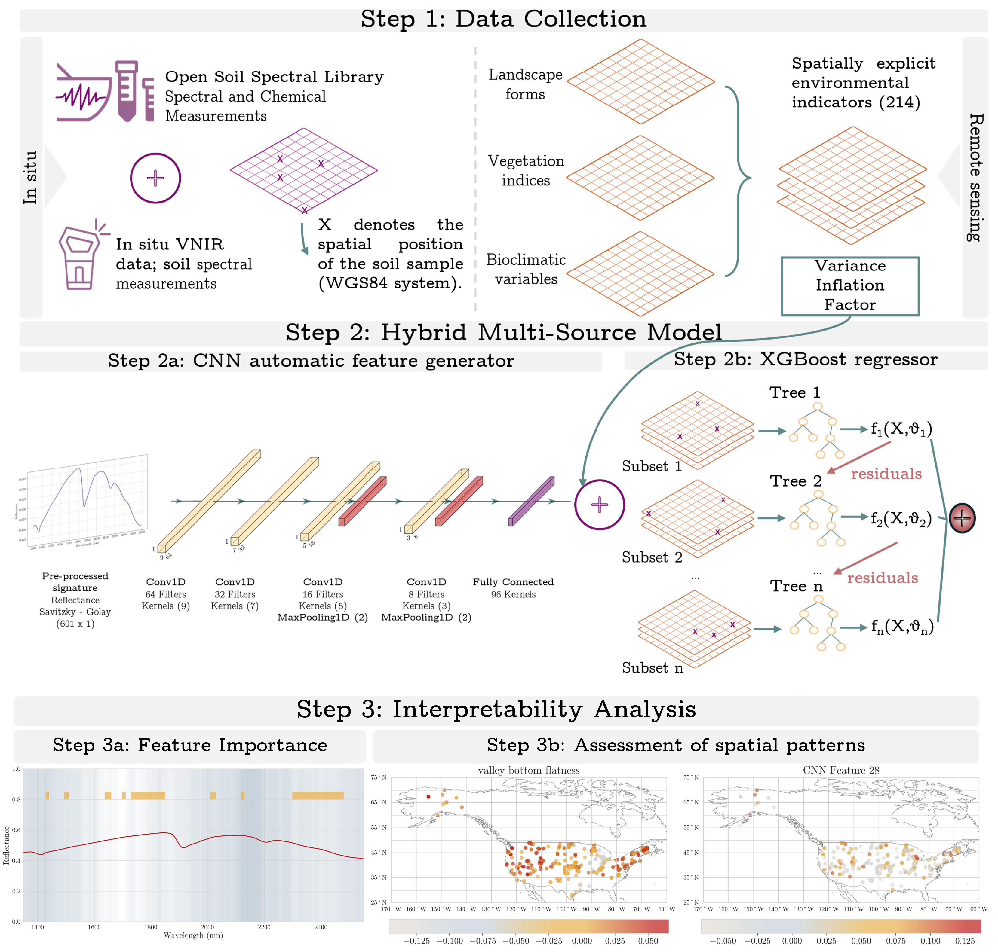
The methodological approach of our study comprises three steps: (i) data collection; (ii) regression analysis based on a hybrid regression model; and (iii) a post hoc analysis where we evaluate the model’s interpretability and the spatial assessment of its predictions. An overview of the proposed workflow is presented in Figure 1.

2.1. Soil Data

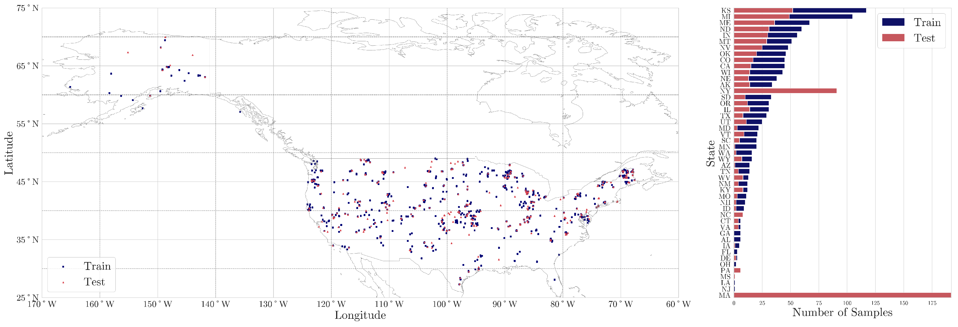
This study utilizes publicly available datasets derived from previous research initiatives. Specifically, the Neo-Spectra NIR database [26], which is readily accessible through the Open Soil Spectral Library (explorer.soilspectroscopy.org), accessed on 13 March 2024, was employed. The selected dataset in this study comprises a collection of 1706 soil samples from across the United States of America (Figure 2) with analytical data on SOC content. These samples were split into train (1202) and test (504) sets, with a ratio of 70%:30%. In addition, our study incorporated a second distinct test set of 269 samples collected from various farms across Massachusetts and New York states, in the years 2021 and 2022, respectively, thus bringing the total number of test samples to 773. All soil samples are given here with precise location coordinates, specified in the WGS84 format. The main training set was chosen to represent the diversity of mineral soil properties found in the United States [26] while the local farm test sets were provided as part of a Kaggle soil spectroscopy competition to find novel ways of utilizing a national spectral library at the local scale [27] (Figure 2). Therefore, the distribution of samples was not a design choice made in this current study.

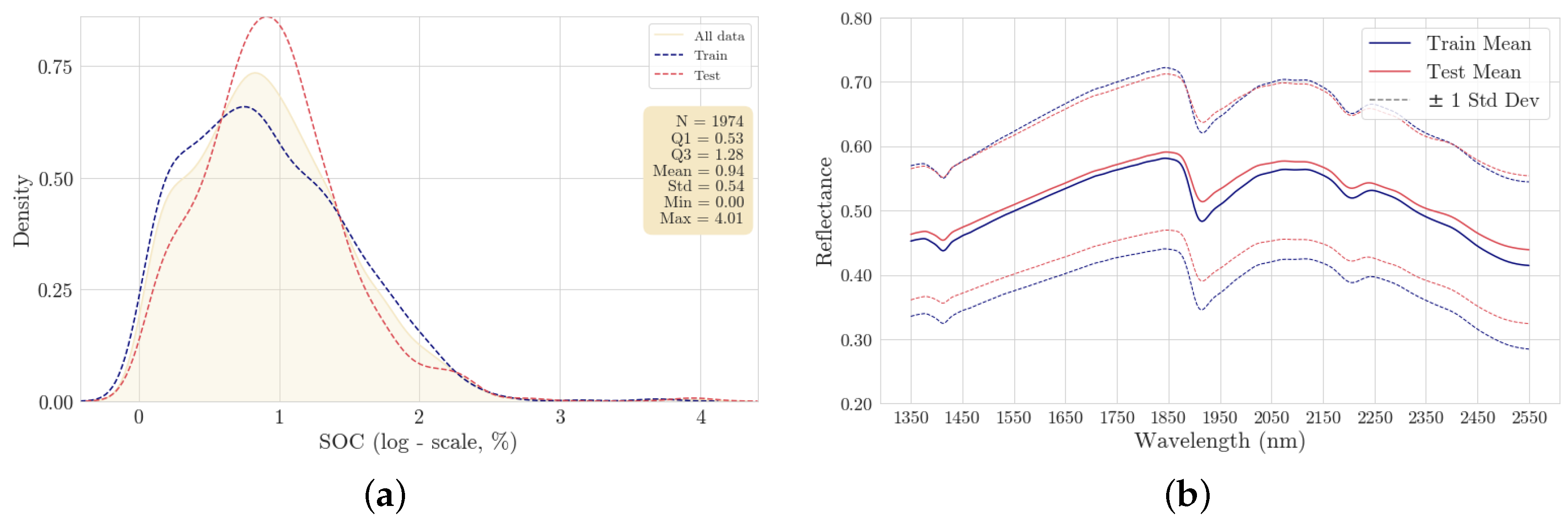
The SOC content was determined as the difference between total carbon, measured using dry combustion, and calcium carbonate, measured by a pressure calcimeter [28]. Overall, it exhibits a highly skewed probability distribution as naturally expected. Therefore, the representation of SOC content is adjusted to a logarithmic scale (taking the natural logarithm with offset 1), as presented in Figure 3a for both the train and test sets. All samples were accompanied by precisely measured spectra covering the wavelength range of 1350 to 2550 nm. These measurements contained 258 records, which were interpolated to 2 nm resolution, resulting in the final format of 601 spectral features. A white reference material was used with the Neo-Spectra sensor for scanning calibration. A comparative plot of the mean reflectance spectra for both train and test sets, including their standard deviations, is presented in Figure 3b, allowing us to visually assess the variability and consistency across the spectral signatures captured with the Neo-Spectra sensor (Si-Ware Systems, Cairo, Egypt). Similar patterns can be observed between train and test datasets.

2.2. Environmental Covariates

A set of 214 spatial layers was available as open geo-environmental covariates for this study, encompassing landform characteristics, climatic dynamics, and vegetation indices, to capture the multifaceted environmental influences on SOC. Landform and landscape information was also used since it provides crucial insights into terrain features that influence SOC distribution. Climatic information derived from BioClim v1.2, with a mean aggregated over 1981–2010 (CHELSA-climate) [29], offered comprehensive temperature and precipitation patterns, supplemented by dynamic overlays of monthly aggregated water vapor and land surface temperature dynamics, along with long-term daytime and nighttime temperatures from 2000 to 2020. Lastly, the cropland spatial distribution from the previous work by Cao et al. [30] was also used.

Table A1. Geo-covariates considered in the present study.

Description	Code Name	Source
Landforms present based on terrain classification (%)	lf.alluvial.pediplain_terrain	[57]
Very gentle landforms based on terrain classification (%)	lf.alluvial.or.coasttal.plain.gentlest.lake.plain.playa_terrain	[57]
Landforms in alluvial or coastal plains/pediplains (%)	lf.alluvial.or.coast.pediplain_terrain	[57]
Landforms specifically in alluvial plains/pediplains (%)	lf.alluvial.plain.pediplain_terrain	[57]
Dissected terraces and moderate plateaus present (%)	lf.dissected.terrace.moderate.plateau_terrain	[57]
Rough hills on both small and large scales (%)	lf.hills.rough.in.small.and.large.scale._terrain	[57]
Middle to large slopes present (%)	lf.middle.large.slope_terrain	[57]
Moderately elevated, rough mountains present (%)	lf.moderate.mountain.rough_terrain	[57]
Smooth, moderate mountains present (%)	lf.moderate.mountain.smooth_terrain	[57]
Slopes in and around terraces or plateaus present (%)	lf.slope.in.and.around.ter_terrain	[57]
Steep and rough mountains present (%)	lf.steep.mountain.rough_terrain	[57]
Smooth, steep mountains present (%)	lf.steep.mountain.smooth_terrain	[57]
Smooth terraces and plateaus present (%)	lf.terrace.smooth.plateau_terrain	[57]
Upper parts of large slopes present (%)	lf.upper.large.slope_terrain	[57]
Categorical classification of various landforms	lf_terrain	[57]
Mean frequency of bare surfaces detected by Landsat	bare.surface_landsat.frequency	[57]
Mean downslope curvature derived from MERIT DEM	downslope.curvature_merit.dem	[57]
Upstream area from MERIT hydrological data (Log1p)	log1p.upstream.area_merit.hydro	[57]
Mean positive openness value derived from MERIT DEM	pos.openess_merit.dem	[57]
Mean slope value derived from MERIT DEM	slope_merit.dem	[57]
Mean upslope curvature derived from MERIT DEM	upslope.curvature_merit.dem	[57]
Valley bottom flatness derived from MERIT DEM	vbf_merit.dem	[57]
Categorical, wetlands associated with UPMC dataset (%)	wetlands.cw_upmc.wtd	[57]
Groundwater-driven wetlands from UPMC dataset (%)	wetlands.groundwater-driven_upmc.wtd	[57]
Aggregation of monthly snow probability	snow.prob_esacci.m	[57]
Water vapor monthly	wv_mcd19a2v061.seasconv	[57]
MODIS LST monthly in daytime or nighttime	clm_lst_mod11a2.{day or night}time	[57]
Permanent wetlands from UPMC dataset (%)	wetlands.permanent_upmc.wtd	[57]
Long-term aggregation of monthly MODIS EVI	monthly.evi_mod13q1.v061.m	[57]
Flooded wetlands from UPMC dataset (%)	wetlands.regularly-flooded_upmc.wtd	[57]
Mean diurnal range of temperatures averaged (1981-2010)	bioclim.var_chelsa.bio2	[29]
Ratio of diurnal to annual variation in temperatures	bioclim.var_chelsa.bio3	[29]
Mean monthly precipitation of the wettest quarter	bioclim.var_chelsa.bio16	[29]
Accumulated precipitation amount	bioclim.var_chelsa.bio12	[29]
Precipitation of the wettest month	bioclim.var_chelsa.bio13	[29]
CHELSA rainfall V2.1 monthly	CHELSA_pr_month_year_V.2.1	[29]
Cropland percent at 1km resolution	lcv_globalcropland_bowen.et.al_p	[30]
HILDA+ forest percent at 1km resolution	lcv.forest_hilda_dv1	[58]

in Appendix A summarizes the geo-covariates used in this work.

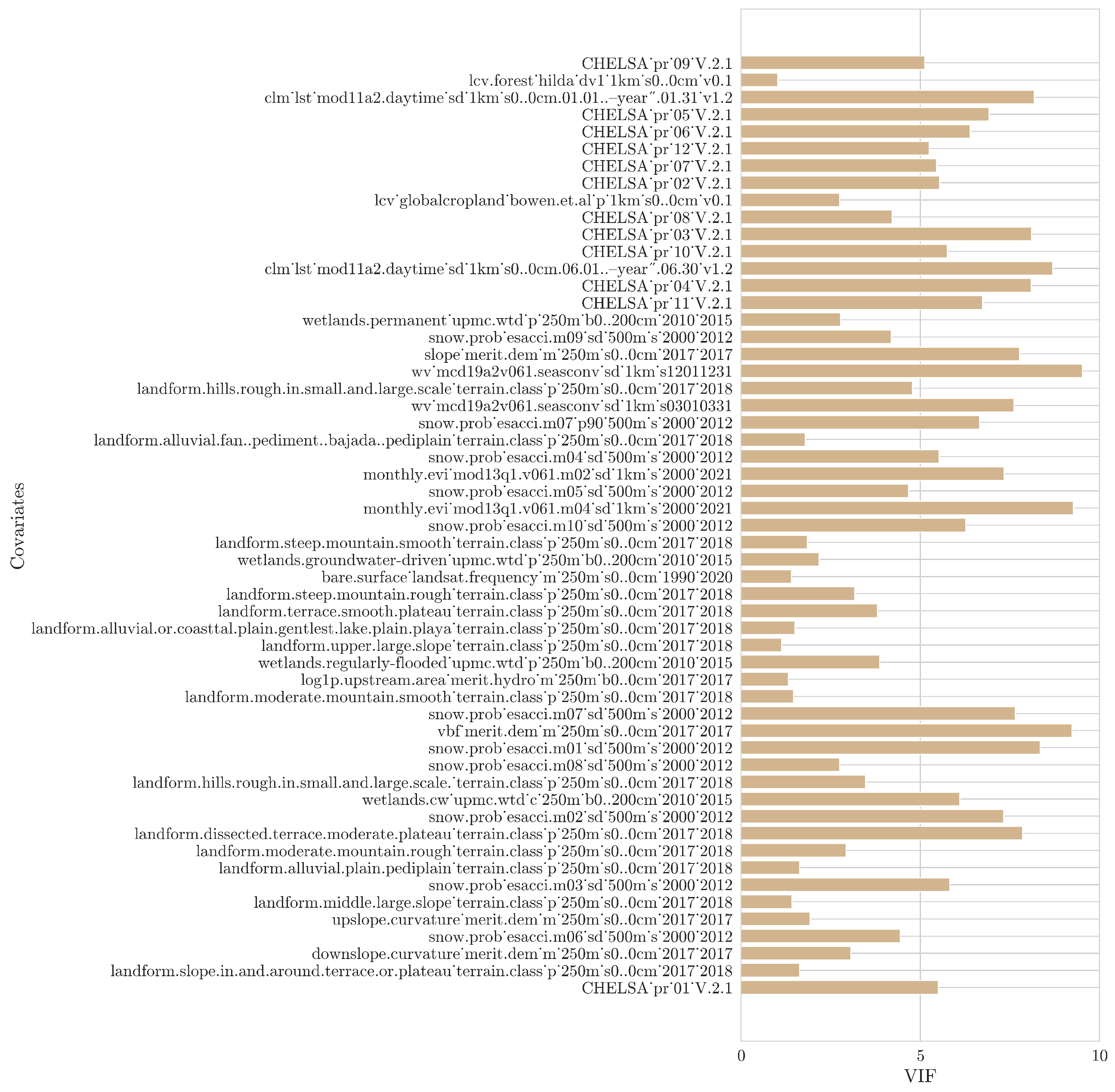
2.3. Addressing Multicollinearity

In order to eliminate the impact of multicollinearity amongst the environmental covariates, we utilized the variance inflation factor (VIF) analysis [31]. The multicollinearity is measured by performing a regression with each covariate against all other covariates in order to derive multiple correlation coefficient values. These values are utilized to calculate the VIF as expressed in Equation (1):

$${\mathrm{VIF}}_i={\displaystyle \frac{1}{1-R_i^2}}$$

(1)

where $R_i^2$ is the coefficient of determination obtained by regressing the i-th predictor against all other predictors.

Subsequently, following a stepwise backward approach, the covariate with the highest VIF value was removed based on a specific cutoff value. A VIF of value one indicates no collinearity between the covariates; however, the threshold value is subjective and depends on the research aim. Based on previous studies, threshold values range from 5 to 10 to ensure a moderate correlation [32]. A threshold of five has been selected in the current work.

2.4. Analysis Using Artificial Intelligence

It is important to highlight that spectral data and geo-covariates are distinct and heterogeneous in nature; hence, it is necessary to tailor our modeling approaches to maximize their predictive performance as well as their interpretability. Spectral data, being sequential and continuous, are ideal for feature extraction with CNNs, which excel at identifying complex patterns and achieving high accuracy on structured datasets. On the other hand, geo-covariates used in this study, such as climatic indices, and topographic variables, have diverse natures and lack a sequential structure required for CNNs to effectively process them. Applying a CNN to these heterogeneous data can hinder performance and interpretability.

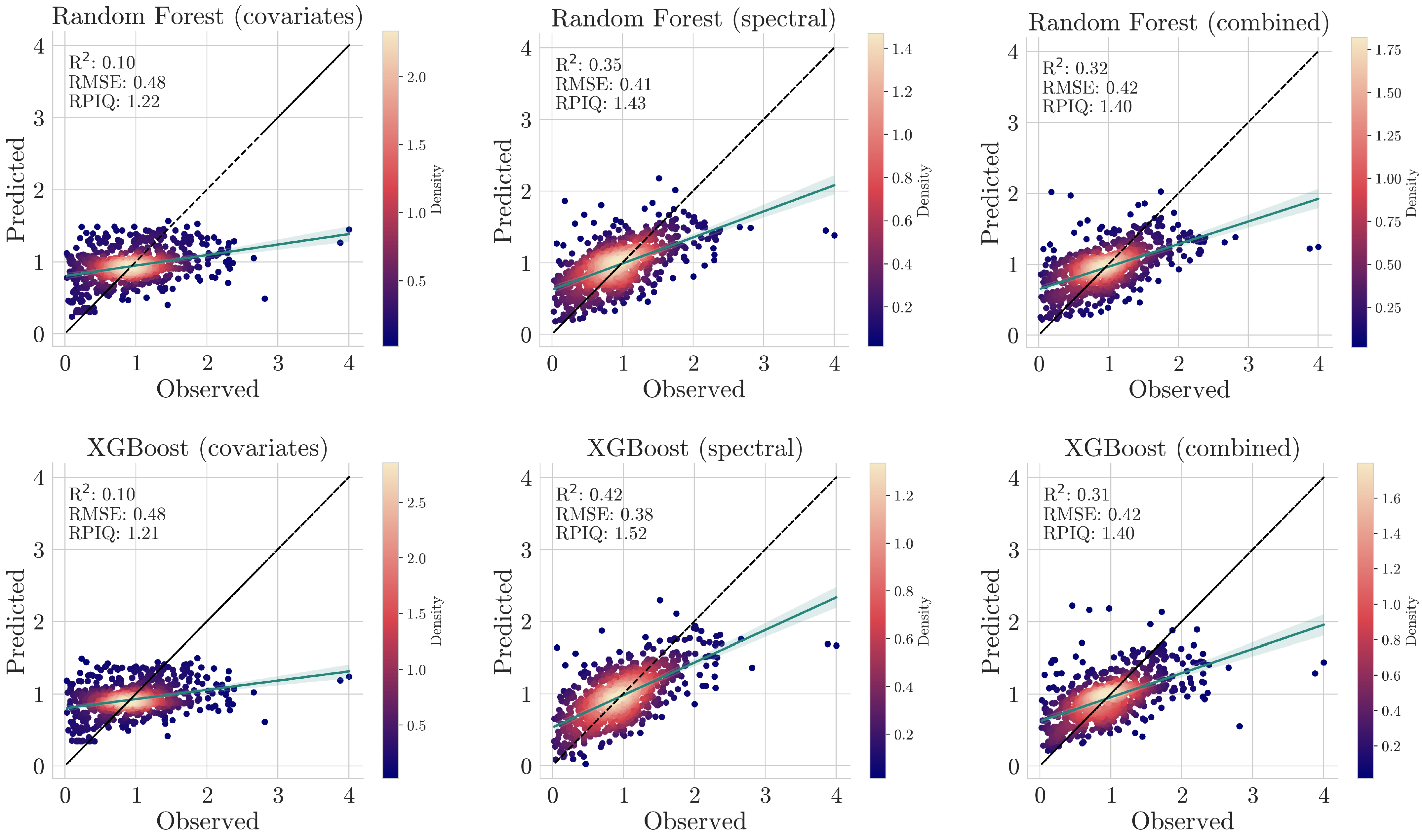
To address these challenges, a hybrid approach was adopted, where CNNs were used to extract features from spectral data that were integrated with other environmental covariates via machine learning models like Random Forests and XGBoost. To establish a baseline for comparison, we tested the performance of machine learning models on spectral data alone, geo-covariates alone, and the combined dataset. However, as previously explained, CNNs are not suitable for modeling covariates or combined data. Therefore, as an extra step, CNNs were applied exclusively to spectral data, allowing for a performance comparison between deep learning and traditional machine learning approaches.

In this section, we describe the architecture of the CNN and the ensemble learning methods (i.e., XGBoost and Random Forest) used for regression in the hybrid approach and as a standalone regressor for comparison with the proposed approach.

2.4.1. Description of the CNN Architecture

CNN, as an automatic feature generator, is initiated with an input layer designed to accept one-dimensional spectral recordings with a length of 601 (see Section 2.1). Through an iterative refining probabilistic approach, namely the Tree-structured Parzen Estimator (TPE) algorithm [33] and five-fold cross-validation, we evaluated the most promising hyperparameter configurations. Following the input layer, three convolutional layers with kernel sizes of 7 × 1, 5 × 1, and 3 × 1, respectively, each followed by Leaky ReLU activation functions, were used. These convolutional layers utilize 64, 32, and 16 filters, respectively. Subsequently, max-pooling layers with kernel sizes of 2 × 1 were applied to downsample the features’ generated information from the first convolutional layer. Following the pooling layers, two additional convolutional layers with kernel sizes of 3 × 1 and 8 filters, and 2 × 1 and 1 filter, respectively, continued the feature extraction process. Finally, the feature maps were flattened and passed through a fully connected layer with 128 neurons, employing Leaky ReLU activation functions. The CNN’s architecture is given in

Table 1. CNN model architecture. The light gray line indicates that this part of the architecture is used when the model is applied for regression.

Layer Type	Kernel Size	Filters	Activation
Convolutional	7 × 1	64	Leaky ReLU
Convolutional	5 × 1	32	Leaky ReLU
Convolutional	3 × 1	16	Leaky ReLU
Max-Pooling	2 × 1	-	-
Convolutional	3 × 1	8	Leaky ReLU
Max-Pooling	2 × 1	-	-
Flatten	-	-	-
Fully Connected	-	128	Leaky ReLU
Fully Connected	-	1	tanh

. The model was trained for a maximum number of 2000 epochs or if no further improvement in the accuracy of the validation set was noticed for 50 epochs (plateau). The model converged at 253 epochs. The best hyperparameters to ensure efficiency and effectiveness in the proposed network are listed in

Table A2. Hyperparameters of the CNN architecture.

Hyperparameter	Explored Values
Learning Rate (lr)	$[0.0001,0.001]$
Batch Size (batch_size)	$[16,32,64,128]$
Filters for Conv1D Layer 1 (filters_1)	$[48,64,128]$
Kernel Size for Conv1D Layer 1 (kernel_size_1)	$[7,9]$
Filters for Conv1D Layer 2 (filters_2)	$[16,32]$
Kernel Size for Conv1D Layer 2 (kernel_size_2)	$[5,7]$
Filters for Conv1D Layer 3 (filters_3)	$[8,16]$
Kernel Size for Conv1D Layer 3 (kernel_size_3)	$[3,5]$
MaxPooling1D after Conv1D Layer 1 (pooling_1)	$[\mathrm{True},\mathrm{False}]$
MaxPooling1D after Conv1D Layer 2 (pooling_2)	$[\mathrm{True},\mathrm{False}]$

.

2.4.2. Ensemble Learning Models

We implemented both Random Forest (RF) and Extreme Gradient Boosting (XGBoost) regression models to estimate SOC from spectral recordings and the selected geo-covariates after the VIF approach (Section 2.3). They are considered nonparametric regression models that are able to capture nonlinear relationships among the input features and minimize the risk of over-fitting by combining many trees operating with different feature subsets that are randomly selected. RF is an ensemble learning method that constructs a multitude of decision trees during training and returns the mean prediction of the individual trees [34]. XGBoost is an efficient and scalable implementation of gradient boosting. Similarly to Random Forest, it builds a series of decision trees sequentially; however, each subsequent tree adjusts the errors made by the previous one at each step, resulting in a powerful ensemble model [35].

Both Random Forest and XGBoost were optimized using a Bayesian approach in a five-fold cross-validation of the calibration set (i.e., where each evaluation of the set of hyperparameters is evaluated across the five folds) to systematically fine-tune their hyperparameters toward the maximization of the model’s predictive performance. We explored a range of values for each hyperparameter. We also tested different strategies for selecting the maximum features at each split, specifically using the square root ($\sqrt{M}$) and base-2 logarithm (${log}_2\left(M\right)$) of the total number of features, where M represents the total feature count. Similarly, for XGBoost, we applied Bayesian search to optimize hyperparameters, including maximum tree depth, learning rate, the number of estimators, column subsample ratio, and $L_1$ regularization strength, ensuring a thorough evaluation of parameter values to maximize predictive accuracy. Briefly, in Random Forest, we evaluated the number of estimators within the range of 50 to 1000, testing maximum depth values from 3 up to 20 with a step of 1, and applying feature selection strategies that use the square root or base-2 logarithm of the total features. For XGBoost, we assessed tree depth values between 3 and 8, learning rates within {0.01, 0.05, 0.1, 0.2}, the number of estimators ranging from 10 to 1000, subsample ratios of [0.3–0.8, by step 0.1], and regularization strengths with L1 penalty values of 0, 5, and 10. We optimized hyperparameters for each dataset (spectral, geo-covariates, and combined) to tailor the models to their specific characteristics. Hence, the final models were trained using different configurations of optimized hyperparameters, tailored to each dataset and model to ensure an alignment with the specific characteristics of the spectral, the selected geo-covariates from the VIF approach, and combined datasets. All results, including hyperparameters and performance metrics, are summarized in

Table A3. Random Forest hyperparameters.

Description	Hyperparameters
Geo-covariates	Max Depth: 30, Max Features: sqrt, Estimators: 150
Spectral	Max Depth: 20, Max Features: sqrt, Estimators: 100
Combined	Max Depth: 70, Max Features: log2, Estimators: 250

for Random Forest models and

Table A4. XGBoost hyperparameters.

Description	Hyperparameters
Geo-covariates	Learning Rate: 0.05, Max Depth: 8, Estimators: 50, Subsample: 0.4, Gamma: 0
Spectral	Learning Rate: 0.05, Max Depth: 6, Estimators: 500, Reg_Alpha: 1, Subsample: 0.5, Gamma: 0
Combined	Learning Rate: 0.01, Max Depth: 3, Estimators: 1000, Subsample: 0.6, Gamma: 0.5

for XGBoost models, while the results for the hybrid models are presented in

Table A5. CNN-Random Forest and CNN-XGBoost hyperparameters.

Model	Hyperparameters of Hybrid Models
Random Forest	Max Depth: 30, Max Features: sqrt, Estimators: 200
XGBoost	Learning Rate: 0.12, Max Depth: 5, Estimators: 120, Subsample: 0.8

.

2.5. Interpretability

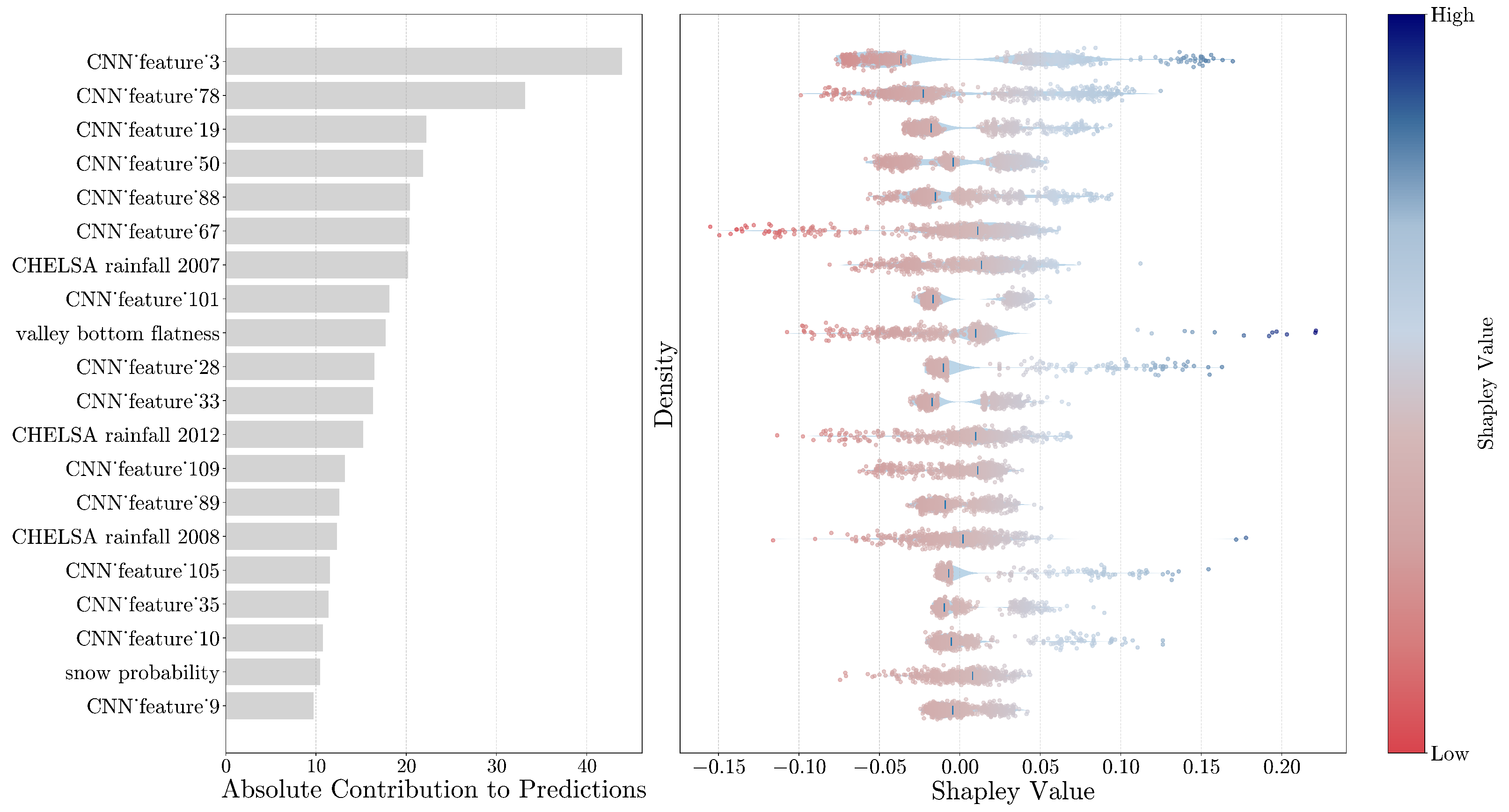
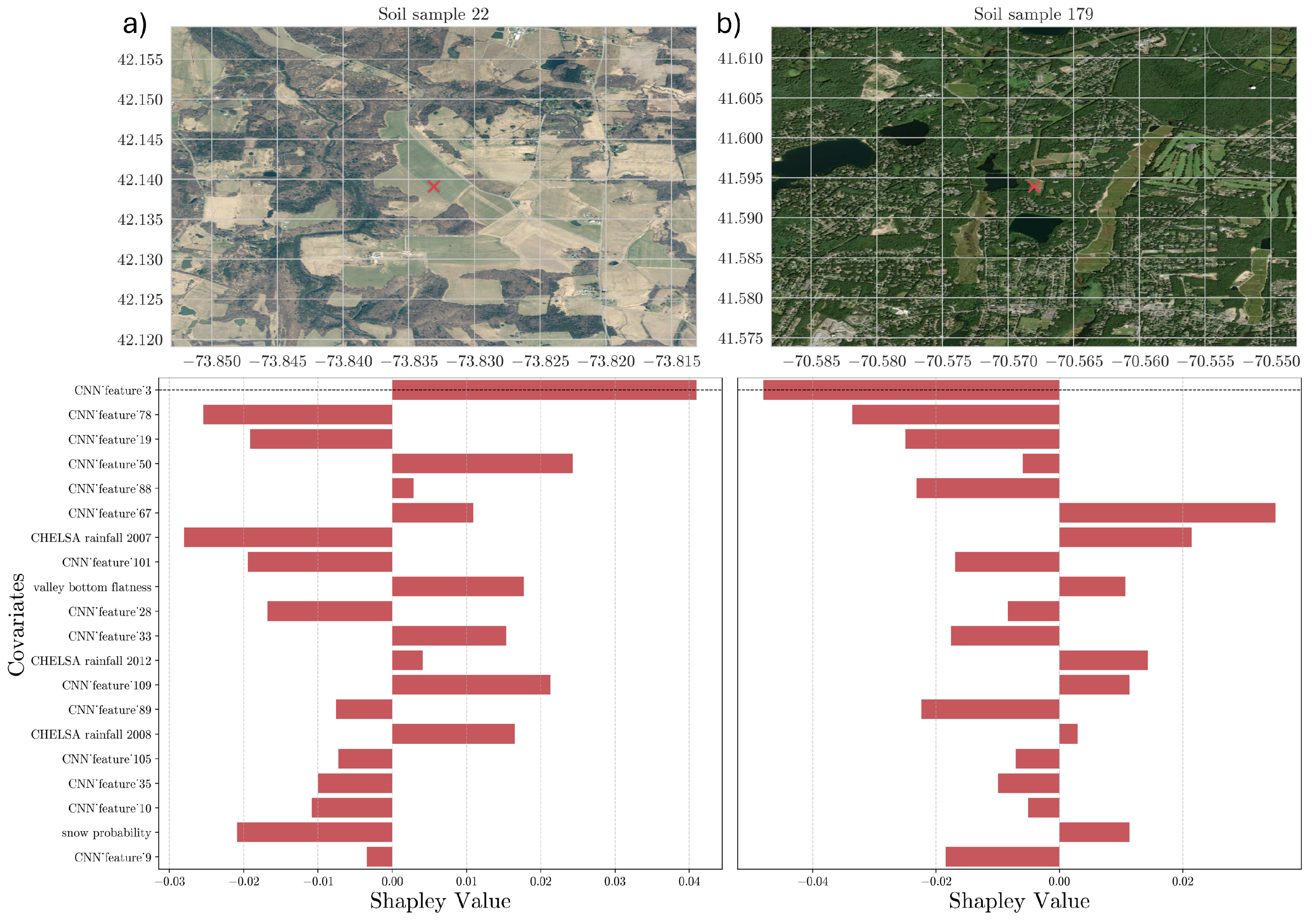
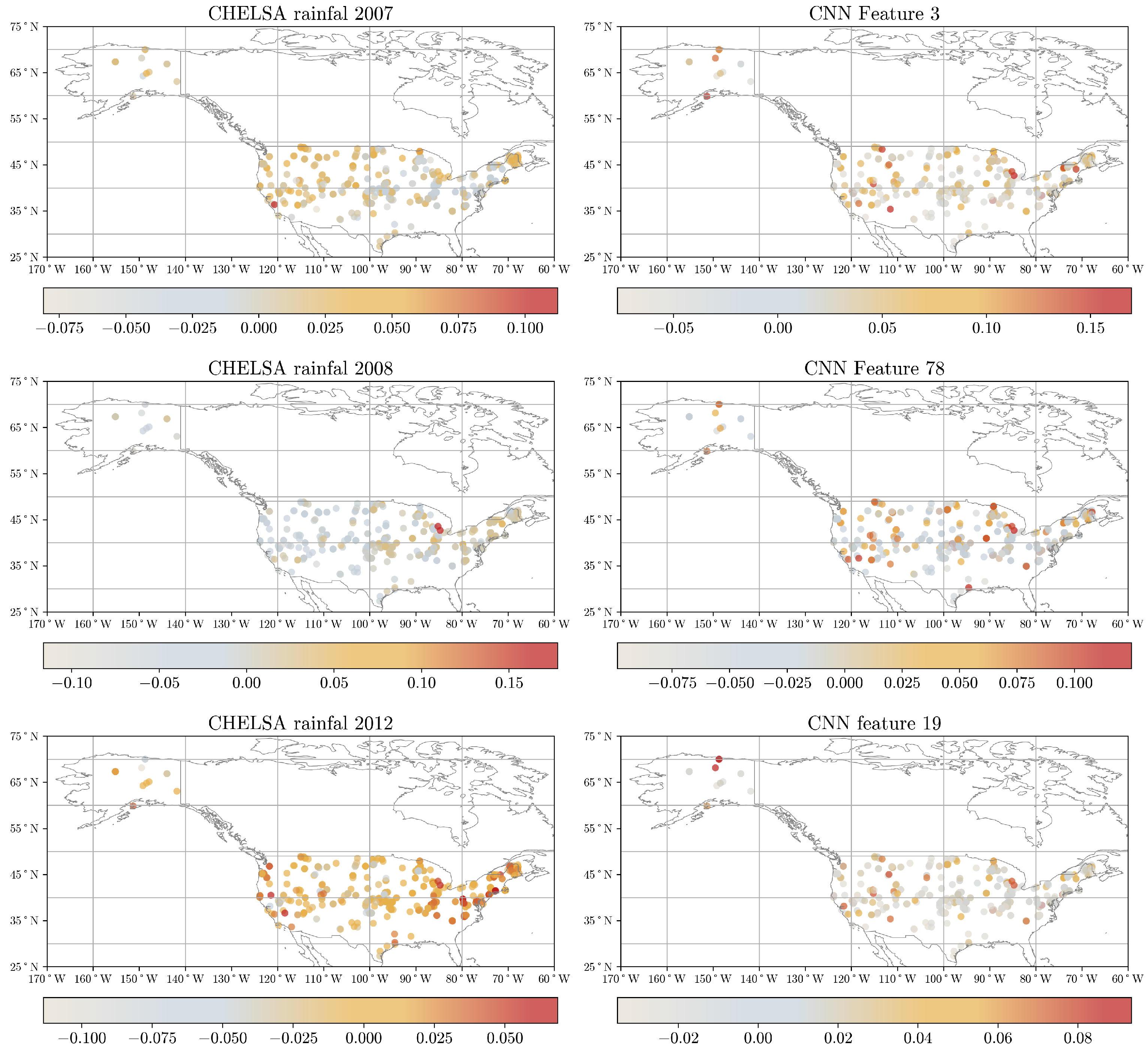
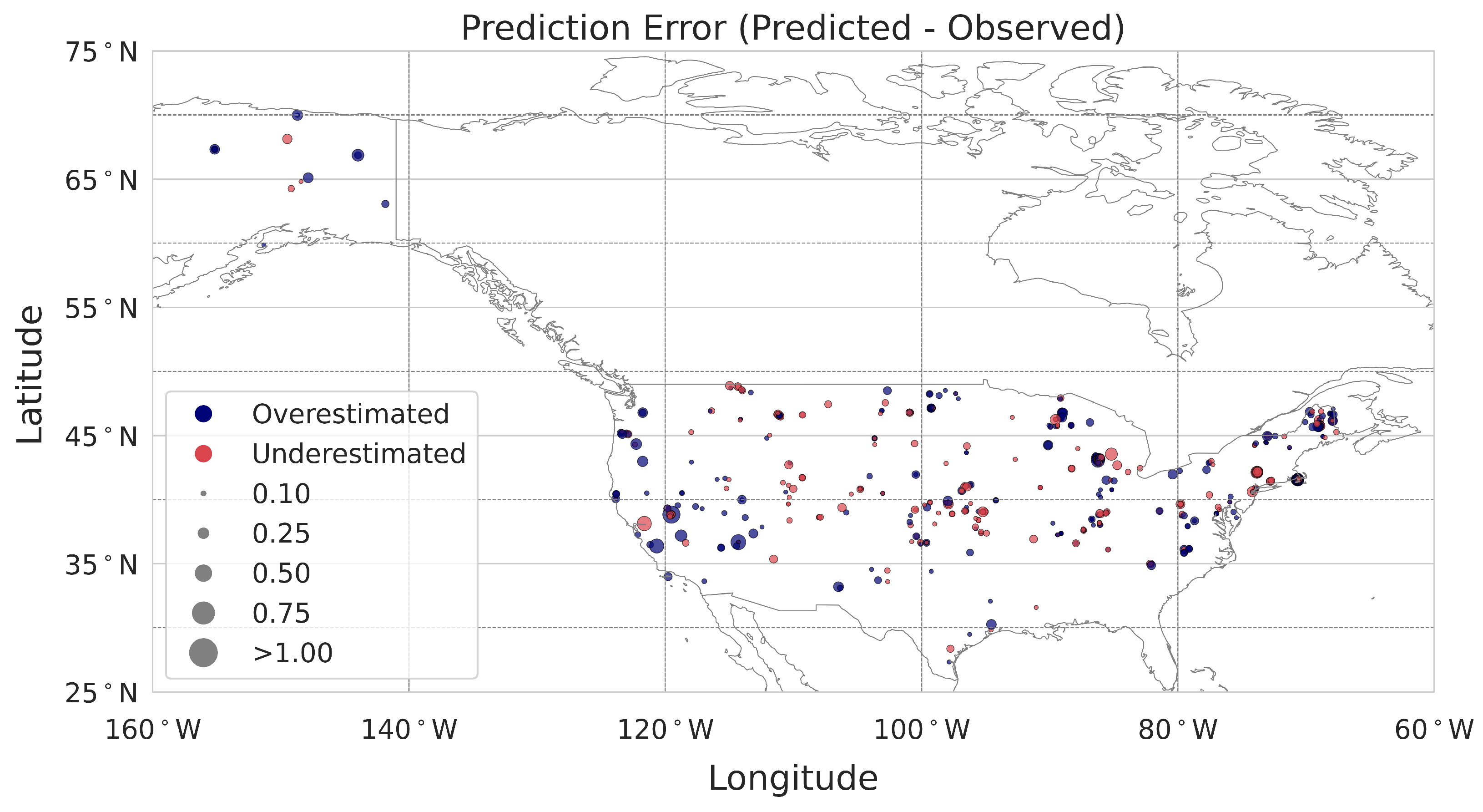
Shapley values were used to estimate how the input features, considering both the generated features from the CNN and the geo-covariates, affect the SOC predictions. Shapley values are one of the most used explainability techniques for ranking the input features and estimating their contribution to the model’s predictions per instance [36]. The importance of each predictor is properly weighted by considering the interactions between input features. Moreover, we derived the average contribution by summing the absolute Shapley values across individual observations in the calibration dataset, resulting in an overall variable contribution to the prediction. Lastly, we evaluated the contribution of each point considering spatial patterns that can help us to determine the average contribution for specific areas, such as bioclimatic regions or states across the USA.

Moreover, we further explored techniques to gain insights into the reasoning process of the CNN model. In this regard, the feature maps created at each convolution layer capture complex features, with the final layer retaining a strong correlation between each neuron’s position and the input wavelength. This allowed us to assess the spectral region that mostly drives the model’s estimations, enabling us to confirm the model’s alignment with areas corresponding to well-known chemical bonds impacting SOC. This comparison reinforces the interpretability of our approach.

2.6. Evaluation

The coefficient of determination ($R^2$, Equation (2)) assesses how well the independent variables explain the variability of the dependent variable. Root Mean Square Error (RMSE, Equation (3)) measures the average difference between predicted and observed values, while the Ratio of Performance to Interquartile Range (RPIQ, Equation (4)) evaluates model performance relative to data quartiles. The metrics above have been calculated using the following equations:

$$R^2=1-{\displaystyle \frac{{\sum }_{i=1}^n{(y_i-{\widehat{y}}_i)}^2}{{\sum }_{i=1}^n{(y_i-\overline{y})}^2}}$$

(2)

$$RMSE=\sqrt{{\displaystyle \frac{1}{n}}\sum _{i=1}^n{(y_i-{\widehat{y}}_i)}^2}$$

(3)

$$RPIQ={\displaystyle \frac{\mathrm{IQ}}{\mathrm{RMSE}}}$$

(4)

where $y_i$ denotes the observed values, ${\widehat{y}}_i$ stands for the predicted values, $\overline{y}$ denotes the mean of observed values, RMSE denotes Root Mean Square Error, n represents the number of observations, and $\mathrm{IQ}=Q3-Q1$ indicates the interquartile range of the observed values.

2.7. Computational Framework

Data processing and regression analysis were performed on HiPerGator 3.0 (UFIT Research Computing, Gainesville, FL, USA), a high-performance computing cluster at the University of Florida, using an NVIDIA RTX 2080 Ti GPU (NVIDIA Corporation, Santa Clara, CA, USA). The code for the AI modeling is based on the Python libraries scikit-learn, TensorFlow, and Keras. All experiments and computations for the calculation of Shapley values were conducted using the SHAP package in Python programming language [37].

3. Results

3.1. SOC Estimation

Figure 4 presents a comparison of the performance metrics in the independent test set for the Random Forest and XGBoost models applied to the spectral data, selected geo-covariates by VIF, and the combined dataset. It should be noted that 37 features remained after reducing the multicollinearity, representing a percentage of 17.29% of the total (214) dataset. The selected covariates are presented in Figure A1.

For the combined dataset, XGBoost and Random Forest achieved similar predictive metrics with an RMSE equal to 0.42% log-SOC and an RPIQ equal to 1.40. For the Spectral dataset, XGBoost achieved better results across all metrics ($R^2$ of 0.42, RMSE of 0.38 log-SOC, and RPIQ of 1.52) compared to Random Forest ($R^2$ of 0.35, RMSE of 0.41 log-SOC, and RPIQ of 1.43). Lastly, using only the geo-covariates, this type of modeling yielded the lowest predictive performance across the test sets while the models’ explained variance showed that the difference between the two learning algorithms was minimal; both Random Forest and XGBoost attained an ($R^2$ of 0.10 and an RMSE equal to 0.48 log-SOC in both cases, while the RPIQ metrics were slightly different, with 1.22 and 1.21. Overall, this evaluation and the regression plots (Figure 4) confirm that XGBoost and Random Forest provided similar predictive capabilities across the test set evaluated; however, high values of SOC are always underestimated.

Following the initial evaluations, we next examined the performance of the CNN architecture (Table 1) synergistically with the Random Forest and XGBoost models. In brief, the CNN alone using only the spectral values achieved an $R^2$ of 0.62, with an RMSE of 0.31 log-SOC and an RPIQ of 1.87. When we integrated the geo-covariates along with Random Forest, the hybrid model’s performance improved, resulting in an $R^2$ of 0.70, an RMSE of 0.28 log-SOC, and an RPIQ of 2.12. Notably, hybrid CNN with XGBoost yielded the highest performance metrics, achieving an $R^2$ of 0.72, an RMSE of 0.27 log-SOC, and an RPIQ of 2.17, a 2.36% decrease compared to the CNN-Random Forest model. The regression plots are summarized in Figure 5.

3.2. Spatial Distribution of SOC Estimations

In this section, we focus on the results from the best model identified in the previous section, specifically the CNN-XGBoost model. Subsequently, to evaluate the spatial distribution of estimation errors, we visualized the differences between observed and predicted values, and we presented a geographic distribution map of the prediction error (Figure 6). This visualization highlights the spatial variation in model performance across different regions. Overall, the models demonstrate a similar pattern of accuracy when comparing the observed with the predicted values. However, differences in certain areas, such as Alaska, suggest potential limitations in the model’s performance in those regions.

3.3. Interpretability

In Figure 7, we visualize the mean activation map of the first convolutional layer of the CNN feature generator. Furthermore, to enhance the interpretability of the results, we overlay the mean activation values with the mean reflectance spectral signature of the training dataset, while important spectral regions corresponding to specific chemical bonds, such as O–H, C–H, and C=O overtones [38], are highlighted with a horizontal yellow rectangular shape. The positions of the most important absorption features of soil organic matter in the reflectance spectrum have been extensively discussed in the literature, particularly in relation to the main infrared absorption characteristics of organic components [39,40].

The activation plot is presented to highlight the spectral regions where the CNN model, acting as a feature generator, concentrates during training. More specifically, the denser regions in the plot indicate the wavelengths with higher activation frequencies, suggesting that these areas are more influential in the model’s decision-making process. Based on this analysis, we can gain insights into which parts of the spectrum are most relevant during the feature extraction process. The final convolutional layer has been selected for the analysis.

The SHAP analysis plot in Figure 8 provides a clear visualization of how the distinct data sources, spectra denoted as CNN features, and geo-covariates contribute to the hybrid model’s estimations. This visual comparison allows for an easy assessment of the direction and strength of influence each feature has on the final estimation, helping to reveal which data source plays a greater or less-significant role in guiding model outcomes.

The mean absolute Shapley values plot in Figure 8 illustrates the contribution level of spectral information and geo-covariates to the estimation of SOC, averaged over the calibration dataset. By assessing the Shapley values, we observe that the spectral features generated by the CNN (e.g., features 3 and 78) contribute significantly, with average absolute values above 30. Similarly, other spectral features (e.g., features 88 and 50) also have a substantial impact, with average absolute values exceeding 20. Moreover, it is evident that information referring to the rainfall during 2017 (CHELSA rainfall 2007) as well as valley bottom flatness are, on average, the most significant geo-covariates influencing the estimation of SOC, with their average absolute values exceeding 15 in both cases.

Furthermore, the right-hand plot in Figure 8 demonstrates that the four most significant features exhibit a wide range of Shapley values. For example, the rainfall for 2007 has values ranging from $-0.07$ to 0.07. Overall, we observe a positive mean Shapley value for this feature that can justify that it adds to the prediction, pushing the outcome closer to the observed values. On the other hand, spectral feature information generated by CNN (and in particular, CNN features 3, 78, and 19 that are noted as the three most important features) has extreme values ranging from $-0.10$ to 0.16. For these features, we can conclude that their Shapley values indicate that negative contributions mainly occur at lower values since all of them resulted in a negative mean Shapley value. For the rest of the features, the contributions are within a small range, with the majority of the features showing similar trends, apart from CNN features 28 and 105. For example, the layer providing information for the valley bottom flatness of a soil sample also has a significant average contribution to the estimation, having positive contributions for lower values in estimating SOC.

Figure 9 illustrates the contribution of spectral and geo-environmental features of SOC estimations at two different locations within farms in (a) New York (sample 22) and (b) Massachusetts (sample 179). The SOC values were estimated to be 1.01 and 0.71 for samples 22 and 179, respectively, with percentage errors of less than 2% in these locations. However, as we can observe, they have significant differences in the Shapley value estimates between the two locations. In the New York farm, spectral features 3 and 50 emerge among the primary positive contributors to SOC estimations, followed by CHELSA rainfall 2008, as well as spectral feature 33. Conversely, CHELSA precipitation 2007 and spectral information from features 19 and 78 are the leading negative contributors. In Massachusetts, a completely different pattern is noticed, with the first spectral features 3 and 50 being the primary negative contributors, while the precipitation of 2007 stands out as the main positive contributor together with spectral feature 67. In the precipitation of 2007, we observed differences in New York’s pattern. Additionally, 2012 is also a significant positive contributor in this region.

In Figure 10, we illustrate that precipitation has the most significant influence on the estimations, with notable contributions observed during the years 2007, 2008, and 2012. While no specific spatial pattern is apparent for 2007, a strong influence is evident near points close to Lake Erie in 2008. In 2012, a year marked by severe drought across much of North America, the contributions were more pronounced in the eastern and western parts of the continent, highlighting regional variability in precipitation’s impact over time. On the other hand, considering the spectral features, while specific information may not be readily distinguished, there are values showing notable contributions. For instance, samples close to Lake Erie or Alaska reveal significant contributions, underscoring the relevance of localized environmental factors in the predictive framework.

4. Discussion

4.1. Predictions

The results presented in Figure 5 indicate the superiority of deep learning techniques over conventional ML methods, resulting in a decrease of approximately 29.27% in the RMSE compared to Random Forest and XGBoost. These results indicate a significant improvement in predictive accuracy as the multimodal data were combined, with CNN-XGBoost demonstrating the strongest ability to capture the underlying patterns in the data.

In recent years, the use of CNNs in the domain of spectroscopy has been extensively investigated with several works built upon existing architectures [41], having high predictive performance. Although the Neo-Spectra sensor did not capture the visible and near-infrared (NIR) range, its predictive performance for SOC fractions remains satisfactory. The absence of information in the 350–1350 nm range could slightly reduce estimation accuracy compared to works using the full 350–2500 nm VNIR-SWIR spectrum [42], as this range provides critical information on organic carbon-related color and important molecular bonds.

4.2. Impact of Fusion

The spectra are combined with geo-covariates derived from satellites, and the results presented in Figure 5 demonstrate a significant increase in the predictive performance of our models. Overall, we observe a consistent pattern across the states with a few examples such as Alaska and Arizona, where the model tends to overestimate the real values (Figure 6). This discrepancy could be attributed to the limited representation of data points in these regions; hence, the model’s performance is hindered by the lack of sufficient and representative calibration points. Another factor is the potential for bias in environmental covariates that could limit the applicability in areas where extreme environmental conditions may be found. The findings from the single use of geo-covariates and spectral-only features (Figure 4) underscore the impact of data fusion on model performance both for the ensemble learning techniques but also for the hybrid models (Figure 5), highlighting the synergistic relationship between Neo-Spectra and geo-covariates in enhancing predictive capabilities. Kok et al. [24], implemented a fusion of in situ and spaceborne datasets with available soil archives, yielding a 4.69% increase in the RPIQ, compared to the approach where only the spectral recording is utilized. Compared to their work, our model architecture is designed to incorporate multiple data sources, making it adaptable for broader applications. Therefore, we take a step forward by implementing a multimodal framework that allows for flexible data flow, enabling outputs from one stage of the model to be reintroduced later and enhancing predictive performance by integrating heterogeneous data. Similarly, valuable results for soil carbon stock assessment were observed in the work of Van der Voort et al. [43], which employed a hybrid approach that fused satellite data with direct proximal sensing-based soil measurements and utilized Random Forest testing in two states in the USA to estimate soil carbon stocks. In contrast to these recent studies, our approach demonstrates a higher predictive value through the fusion of satellite geo-covariates (Figure 5). This improvement can be attributed to our use of a significant amount of geo-covariates, as derived from the VIF, known to correlate with soil carbon (Table A1). Previous studies mainly used data derived from Sentinel-1, Sentinel-2, digital elevation maps, and ISRIC SoilGrids, while our methodology integrates a broader array of topographical and environmental factors, enhancing the accuracy of soil carbon predictions. This enhanced predictive performance underscores the value of incorporating diverse and comprehensive geo-covariates in soil carbon stock assessment models.

Finally, it is worth noting that this study prioritized fusing remote sensing and laboratory-derived data, excluding field-based information, like soil depth. This aligns with the discussion of Poggio et al. [44] regarding whether sampling depth should be considered as a covariate. Similar work by Ma et al. [45] advised caution when using depth as a covariate considering that the prediction methods and study requirements play a crucial role in determining its effectiveness. Furthermore, depth data in public soil databases are often inconsistent due to variations in sampling protocols and recording practices. Introducing the depth as a covariate could impact model performance and introduce spurious correlations which are not the main focus of this present study.

4.3. Explainability of the Regression Models

Several studies highlight that explainability is crucial in digital soil mapping, since it enables researchers and users to understand the underlying models and decisions, fostering trust in the estimations and facilitating the effective application of results. Tsakiridis et al. [46] and Wadoux et al. [47] proposed interpretation techniques for modeling spectral and environmental data, respectively. Here, we expand on these studies, demonstrating that a few specific spectral and geo-covariate features dominate the explainability of these models.

Considering the utilization of Shapley values from coalitional game theory to analyze and understand the contributions of spectral and geo-covariates to the estimation of SOC made by the Hybrid CNN-XGBoost model, we concluded that spectral, climatic, and topographical variations play a significant role in influencing the final estimations (Figure 8). Similar patterns were revealed by Wadoux et al. [47], where they quantified the functional relationships between SOC stocks and various environmental factors, revealing how their importance varied both locally and across different carbon-landscape zones. Lastly, in our work, there were no obvious patterns in the distribution of important spectral features; however, certain values demonstrate notable contributions. This suggests that localized environmental factors play an important role in the predictive framework, highlighting the relevance of context in understanding the data. Overall, our findings highlight the importance of the synergistic use of spectral and regional climatic factors in shaping the estimations, which can be further supported by the findings (Figure 10).

4.4. Limitations and Future Steps

While our approach demonstrates promising results, it is not without limitations. These mainly stem from the spatial resolution of the geo-covariates, the handling of heterogeneous data, and the constraints of the hybrid deep learning models used. Recognizing these challenges indicates potential ways for future refinements to enhance the accuracy and applicability of the proposed methodology.

In this study, several open geo-covariates were used, but their coarse spatial resolution poses a significant limitation. Many covariates, such as climatic data, correspond to areas spanning several kilometers and may not adequately capture localized variations. This is most important in the case of vegetation indices derived from MODIS data that may reflect mixed effects of multiple land uses within a single pixel. Incorporating higher-resolution data, such as vegetation indices from Sentinel-2 [48], could improve the accuracy and representativeness of the predictions. Additionally, spectral values derived from bare soil reflectance composites, obtained through advanced data mining techniques [49], should be considered, as these have been shown to yield better overall results. Another limitation lies in the constraints of hybrid deep learning models, such as CNNs, in handling diverse data types. While deep learning was utilized here primarily as a feature generator, emerging architectures like vision transformers [50] and sequential transformers offer the potential to combine diverse datasets [51], including time-series environmental covariates. Future work could expand on this by integrating these architectures to handle spectral variables from sensors like Neo-Spectra, while leveraging both temporal climatic data and spatial characteristics of spectral and topographic variables for improved predictions. Addressing these limitations will pave the way for more robust and versatile modeling frameworks.

Despite the progress recorded with the use of CNNs, this family of deep learning algorithms should not be considered the pinnacle of AI-driven soil spectral analytics, and therefore, alternative techniques could also be investigated. One path of improvement could be using self-supervised contrastive learning models [52]. These algorithms can be used to learn spectral representations from recordings without having explicit laboratory measurements and generate pseudo labels by creating positive and negative pairs of unlabeled data. Then, the findings can transit into a supervised component where ground reference samples could be used for fine-tuning. Such unlabeled data could include field measurements captured directly by relevant stakeholders, such as growers, agricultural consultants, and scientists. We have to take into account that with the increasing use of portable devices, the volume of these data is expected to grow significantly in the coming years. Lastly, we have to consider that in our study, we utilized an extensive dataset that includes a variety of relevant open geo-covariates. We proved that our approach offers a more robust and precise estimation of soil carbon stocks, demonstrating the potential for improved environmental monitoring and management practices. However, the data volume and their diverse nature bring to attention the concept of a digital twin for soil monitoring, emphasizing the importance of data assimilation techniques combined with AI, as discussed by Bauer et al. [53]. Consequently, not only are methods like the proposed hybrid regression algorithm necessary, but also efficient pipelines for high-volume and high-speed observational data acquisition and preprocessing. These components are crucial for the effective integration of data from various sources into a coherent framework, often by combining observational data with model predictions to enhance accuracy. Recent studies are advancing in this direction, providing examples of digital twins for terrestrial water cycles; AI modeling offering high-resolution products as a result of remote sensing; and in situ integration [54]. For instance, Tsakiridis et al. [55] conceptualized a Cognitive Soil Digital Twin for monitoring the soil ecosystem. Its potential extends beyond data analysis, prediction, and representation, serving as a versatile tool for scenario analysis. It enables the visualization of diverse environmental impacts, including the effects of climate change and changes in land use or management practices.

Further future areas of application may involve using a similar fusion process, where instead of laboratory spectra, field (in situ) spectral data are used. This would necessitate applying methods to eliminate confounding factors such as soil moisture and structure [56]. This integration could enable real-time monitoring and analysis within agricultural or ecological settings. By utilizing advancements in mobile and cloud-based systems, the in situ spectra could be collected with smartphones and transmitted to the cloud, where they could be fused with other up-to-date geo-covariates to provide accurate point estimates of soil properties.

5. Conclusions

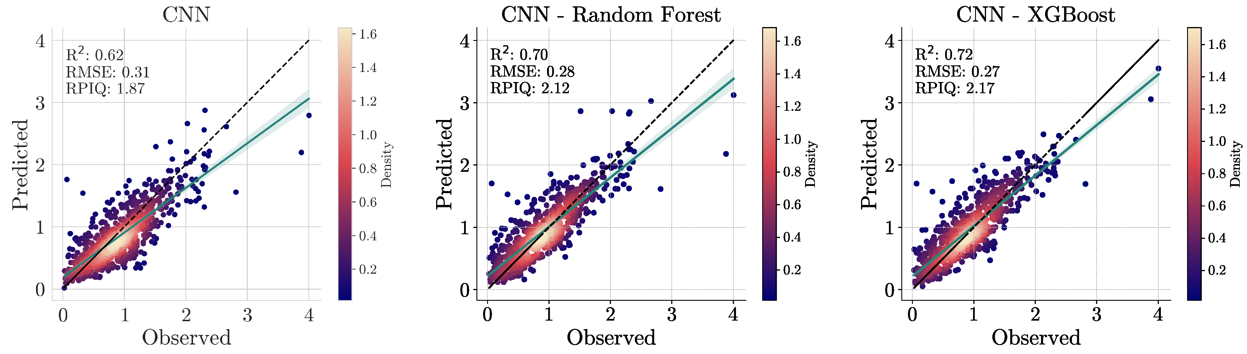
This study exemplifies the synergistic integration of deep learning methodologies and diverse data sources to address the unprecedented challenges in rapid and accurate soil predictions by leveraging and building upon dual-input frameworks. More specifically, we introduced a comprehensive methodological framework for predicting organic carbon in soils using spectral data acquired from a handheld NIR device, combined with open geospatial covariates related to landform, climate, and vegetation. Initial experiments demonstrated that CNNs, utilizing low-cost spectral devices, achieved accurate results with an $R^2$ of 0.62, an RMSE of 0.31, and an RPIQ of 1.87. In this context, the study’s findings emphasize the effectiveness of a hybrid model, using a CNN as an automatic feature generator and an XGBoost as a regression method to handle the multimodal data leading to a remarkable RMSE reduction of >30% and an improved $R^2$ of 0.72, along with an RPIQ of 2.17 compared to a simple XGBoost model. The integration of geo-covariates alongside Neo-Spectra data significantly further enhanced predictive accuracy, surpassing traditional approaches. Lastly, the use of techniques enabling the explainability of the model’s reasoning allowed for a clearer understanding of the contributions of various climatic and topographical factors, as well as spectral data, illuminating the complex interactions that influence SOC variability. In conclusion, this research highlights the promise of advanced analytical frameworks in enhancing our understanding of various soil properties, paving the way for more effective soil management practices at continental extents.

References

1. McBratney, A.; Hartemink, A.E. Define soil. Soil Secur. 2024, 14, 100135. [Google Scholar] [CrossRef]
2. McBratney, A.; Mendonça Santos, M.; Minasny, B. On digital soil mapping. Geoderma 2003, 117, 3–52. [Google Scholar] [CrossRef]
3. Zhou, T.; Geng, Y.; Chen, J.; Liu, M.; Haase, D.; Lausch, A. Mapping soil organic carbon content using multi-source remote sensing variables in the Heihe River Basin in China. Ecol. Indic. 2020, 114, 106288. [Google Scholar] [CrossRef]
4. Chen, S.; Arrouays, D.; Leatitia Mulder, V.; Poggio, L.; Minasny, B.; Roudier, P.; Libohova, Z.; Lagacherie, P.; Shi, Z.; Hannam, J.; et al. Digital mapping of GlobalSoilMap soil properties at a broad scale: A review. Geoderma 2022, 409, 115567. [Google Scholar] [CrossRef]
5. Padarian, J.; Minasny, B.; McBratney, A.B. Using deep learning for digital soil mapping. Soil 2019, 5, 79–89. [Google Scholar] [CrossRef]
6. Wadoux, A.M.C. Using deep learning for multivariate mapping of soil with quantified uncertainty. Geoderma 2019, 351, 59–70. [Google Scholar] [CrossRef]
7. Tziolas, N.; Tsakiridis, N.; Chabrillat, S.; Demattê, J.A.M.; Ben-Dor, E.; Gholizadeh, A.; Zalidis, G.; van Wesemael, B. Earth Observation Data-Driven Cropland Soil Monitoring: A Review. Remote Sens. 2021, 13, 4439. [Google Scholar] [CrossRef]
8. Castaldi, F.; Palombo, A.; Santini, F.; Pascucci, S.; Pignatti, S.; Casa, R. Evaluation of the potential of the current and forthcoming multispectral and hyperspectral imagers to estimate soil texture and organic carbon. Remote Sens. Environ. 2016, 179, 54–65. [Google Scholar] [CrossRef]
9. Diek, S.; Chabrillat, S.; Nocita, M.; Schaepman, M.E.; de Jong, R. Minimizing soil moisture variations in multi-temporal airborne imaging spectrometer data for digital soil mapping. Geoderma 2019, 337, 607–621. [Google Scholar] [CrossRef]
10. Dvorakova, K.; Shi, P.; Limbourg, Q.; van Wesemael, B. Soil Organic Carbon Mapping from Remote Sensing: The Effect of Crop Residues. Remote Sens. 2020, 12, 1913. [Google Scholar] [CrossRef]
11. Gomes, V.C.; Queiroz, G.R.; Ferreira, K.R. An overview of platforms for big earth observation data management and analysis. Remote Sens. 2020, 12, 1253. [Google Scholar] [CrossRef]
12. Zeraatpisheh, M.; Garosi, Y.; Reza Owliaie, H.; Ayoubi, S.; Taghizadeh-Mehrjardi, R.; Scholten, T.; Xu, M. Improving the spatial prediction of soil organic carbon using environmental covariates selection: A comparison of a group of environmental covariates. CATENA 2022, 208, 105723. [Google Scholar] [CrossRef]
13. Witjes, M.; Parente, L.; Križan, J.; Hengl, T.; Antonić, L. Ecodatacube.eu: Analysis-ready open environmental data cube for Europe. PeerJ 2023, 11, e15478. [Google Scholar] [CrossRef] [PubMed]
14. Rosin, N.A.; Demattê, J.A.; Poppiel, R.R.; Silvero, N.E.; Rodriguez-Albarracin, H.S.; Rosas, J.T.F.; Greschuk, L.T.; Bellinaso, H.; Minasny, B.; Gomez, C.; et al. Mapping Brazilian soil mineralogy using proximal and remote sensing data. Geoderma 2023, 432, 116413. [Google Scholar] [CrossRef]
15. Matinfar, H.R.; Maghsodi, Z.; Mousavi, S.R.; Rahmani, A. Evaluation and Prediction of Topsoil organic carbon using Machine learning and hybrid models at a Field-scale. CATENA 2021, 202, 105258. [Google Scholar] [CrossRef]
16. Biney, J.K.M.; Vašát, R.; Bell, S.M.; Kebonye, N.M.; Klement, A.; John, K.; Borůvka, L. Prediction of topsoil organic carbon content with Sentinel-2 imagery and spectroscopic measurements under different conditions using an ensemble model approach with multiple pre-treatment combinations. Soil Tillage Res. 2022, 220, 105379. [Google Scholar] [CrossRef]
17. Zayani, H.; Fouad, Y.; Michot, D.; Kassouk, Z.; Baghdadi, N.; Vaudour, E.; Lili-Chabaane, Z.; Walter, C. Using Machine-Learning Algorithms to Predict Soil Organic Carbon Content from Combined Remote Sensing Imagery and Laboratory Vis-NIR Spectral Datasets. Remote Sens. 2023, 15, 4264. [Google Scholar] [CrossRef]
18. Li, A.; Yao, C.; Xia, J.; Wang, H.; Cheng, Q.; Penty, R.; Fainman, Y.; Pan, S. Advances in cost-effective integrated spectrometers. Light. Sci. Appl. 2022, 11, 174. [Google Scholar] [CrossRef]
19. Sharififar, A.; Singh, K.; Jones, E.; Ginting, F.I.; Minasny, B. Evaluating a low-cost portable NIR spectrometer for the prediction of soil organic and total carbon using different calibration models. Soil Use Manag. 2019, 35, 607–616. [Google Scholar] [CrossRef]
20. Ng, W.; Husnain; Anggria, L.; Siregar, A.F.; Hartatik, W.; Sulaeman, Y.; Jones, E.; Minasny, B. Developing a soil spectral library using a low-cost NIR spectrometer for precision fertilization in Indonesia. Geoderma Reg. 2020, 22, e00319. [Google Scholar] [CrossRef]
21. Priori, S.; Mzid, N.; Pascucci, S.; Pignatti, S.; Casa, R. Performance of a Portable FT-NIR MEMS Spectrometer to Predict Soil Features. Soil Syst. 2022, 6, 66. [Google Scholar] [CrossRef]
22. Mitu, S.M.; Smith, C.; Sanderman, J.; Ferguson, R.R.; Shepherd, K.; Ge, Y. Evaluating consistency across multiple NeoSpectra (compact Fourier transform near-infrared) spectrometers for estimating common soil properties. Soil Sci. Soc. Am. J. 2024, 88, 1324–1339. [Google Scholar] [CrossRef]
23. Shahabi, A.; Nabiollahi, K.; Davari, M.; Zeraatpisheh, M.; Heung, B.; Scholten, T.; Taghizadeh-Mehrjardi, R. Spatial prediction of soil properties through hybridized random forest model and combination of reflectance spectroscopy and environmental covariates. Geocarto Int. 2022, 37, 18172–18195. [Google Scholar] [CrossRef]
24. Kok, M.; Sarjant, S.; Verweij, S.; Vaessen, S.F.; Ros, G.H. On-site soil analysis: A novel approach combining NIR spectroscopy, remote sensing and deep learning. Geoderma 2024, 446, 116903. [Google Scholar] [CrossRef]
25. Barredo Arrieta, A.; Díaz-Rodríguez, N.; Del Ser, J.; Bennetot, A.; Tabik, S.; Barbado, A.; Garcia, S.; Gil-Lopez, S.; Molina, D.; Benjamins, R.; et al. Explainable Artificial Intelligence (XAI): Concepts, taxonomies, opportunities and challenges toward responsible AI. Inf. Fusion 2020, 58, 82–115. [Google Scholar] [CrossRef]
26. Partida, C.; Safanelli, J.; Mitu, S.; Faruk-Murad, M.; Ge, Y.; Ferguson, R.; Shepherd, K.; Sanderman, J. Building a Near-infrared (NIR) Soil Spectral Dataset and Predictive Machine Learning Models using a Handheld NIR Spectrophotometer. Data Brief, 2024; In review. [Google Scholar]
27. Minarik, R. SS4GG Hackathon: NIR Soil Spectroscopy Modelling. 2023. Available online: https://kaggle.com/competitions/ss4gg-hackathon-nir-neospectra (accessed on 10 October 2023).
28. Staff, S.S. Kellogg Soil Survey Laboratory Methods Manual, Version 6.0 ed.; Soil Survey Investigations Report; U.S. Department of Agriculture, Natural Resources Conservation Service: Lincoln, NE, USA, 2022; Volume 42.
29. Karger, D.N.; Conrad, O.; Böhner, J.; Kawohl, T.; Kreft, H.; Soria-Auza, R.W.; Zimmermann, N.E.; Linder, H.P.; Kessler, M. Climatologies at high resolution for the earth’s land surface areas. Sci. Data 2017, 4, 122. [Google Scholar] [CrossRef]
30. Cao, B.; Yu, L.; Li, X.; Chen, M.; Li, X.; Hao, P.; Gong, P. A 1 km global cropland dataset from 10 000 BCE to 2100 CE. Earth Syst. Sci. Data 2021, 13, 5403–5421. [Google Scholar] [CrossRef]
31. O’Brien, R.M. A Caution Regarding Rules of Thumb for Variance Inflation Factors. Qual. Quant. 2007, 41, 673–690. [Google Scholar] [CrossRef]
32. Christopher, G.T.; Rae, S.K.; Becker, B.J. Extracting the Variance Inflation Factor and Other Multicollinearity Diagnostics from Typical Regression Results. Basic Appl. Soc. Psychol. 2017, 39, 81–90. [Google Scholar] [CrossRef]
33. Watanabe, S. Tree-Structured Parzen Estimator: Understanding Its Algorithm Components and Their Roles for Better Empirical Performance. arXiv 2023, arXiv:2304.11127. [Google Scholar] [CrossRef]
34. Breiman, L. Random forests. Mach. Learn. 2001, 45, 5–32. [Google Scholar] [CrossRef]
35. Chen, T.; Guestrin, C. XGBoost: A Scalable Tree Boosting System. arXiv 2016, arXiv:1603.02754. [Google Scholar] [CrossRef]
36. Sundararajan, M.; Najmi, A. The many Shapley values for model explanation. arXiv 2020, arXiv:1908.08474. [Google Scholar] [CrossRef]
37. Hunter, J.D. Matplotlib: A 2D graphics environment. Comput. Sci. Eng. 2007, 9, 90–95. [Google Scholar] [CrossRef]
38. Debaene, G.; Bartmiński, P.; Niedźwiecki, J.; Miturski, T. Visible and near-infrared spectroscopy as a tool for soil classification and soil profile description. Pol. J. Soil Sci. 2017, 50, 1–10. [Google Scholar] [CrossRef]
39. Weyer, L.G. Near-Infrared Spectroscopy of Organic Substances. Appl. Spectrosc. Rev. 1985, 21, 1–43. [Google Scholar] [CrossRef]
40. Lin-Vien, D.; Colthup, N.; Fateley, W.; Grasselli, J. The Handbook of Infrared and Raman Characteristic Frequencies of Organic Molecules; Academic Press: Cambridge, MA, USA, 1991. [Google Scholar]
41. Tsimpouris, E.; Tsakiridis, N.L.; Theocharis, J.B. Using autoencoders to compress soil VNIR–SWIR spectra for more robust prediction of soil properties. Geoderma 2021, 393, 114967. [Google Scholar] [CrossRef]
42. Tang, Y.; Jones, E.; Minasny, B. Evaluating low-cost portable near infrared sensors for rapid analysis of soils from South Eastern Australia. Geoderma Reg. 2020, 20, e00240. [Google Scholar] [CrossRef]
43. van der Voort, T.S.; Verweij, S.; Fujita, Y.; Ros, G.H. Enabling soil carbon farming: Presentation of a robust, affordable, and scalable method for soil carbon stock assessment. Agron. Sustain. Dev. 2023, 43, 22. [Google Scholar] [CrossRef]
44. Poggio, L.; de Sousa, L.M.; Batjes, N.H.; Heuvelink, G.B.M.; Kempen, B.; Ribeiro, E.; Rossiter, D. SoilGrids 2.0: Producing soil information for the globe with quantified spatial uncertainty. Soil 2021, 7, 217–240. [Google Scholar] [CrossRef]
45. Ma, Y.; Minasny, B.; McBratney, A.; Poggio, L.; Fajardo, M. Predicting soil properties in 3D: Should depth be a covariate? Geoderma 2021, 383, 114794, Erratum to Geoderma 2022, 410. [Google Scholar] [CrossRef]
46. Tsakiridis, N.L.; Keramaris, K.D.; Theocharis, J.B.; Zalidis, G.C. Simultaneous prediction of soil properties from VNIR-SWIR spectra using a localized multi-channel 1-D convolutional neural network. Geoderma 2020, 367, 114208. [Google Scholar] [CrossRef]
47. Wadoux, A.M.J.C.; Saby, N.P.A.; Martin, M.P. Shapley values reveal the drivers of soil organic carbon stocks prediction. EGUsphere 2022, 2022, 1–25. [Google Scholar] [CrossRef]
48. Corbane, C.; Politis, P.; Kempeneers, P.; Simonetti, D.; Soille, P.; Burger, A.; Pesaresi, M.; Sabo, F.; Syrris, V.; Kemper, T. A global cloud free pixel- based image composite from Sentinel-2 data. Data Brief 2020, 31, 105737. [Google Scholar] [CrossRef]
49. Heiden, U.; d’Angelo, P.; Schwind, P.; Karlshöfer, P.; Müller, R.; Zepp, S.; Wiesmeier, M.; Reinartz, P. Soil Reflectance Composites—Improved Thresholding and Performance Evaluation. Remote Sens. 2022, 14, 4526. [Google Scholar] [CrossRef]
50. Bazi, Y.; Bashmal, L.; Rahhal, M.M.A.; Dayil, R.A.; Ajlan, N.A. Vision Transformers for Remote Sensing Image Classification. Remote Sens. 2021, 13, 516. [Google Scholar] [CrossRef]
51. Kakhani, N.; Rangzan, M.; Jamali, A.; Attarchi, S.; Kazem Alavipanah, S.; Mommert, M.; Tziolas, N.; Scholten, T. SSL-SoilNet: A Hybrid Transformer-Based Framework With Self-Supervised Learning for Large-Scale Soil Organic Carbon Prediction. IEEE Trans. Geosci. Remote Sens. 2024, 62, 1–15. [Google Scholar] [CrossRef]
52. Park, J.; Gwak, D.; Choo, J.; Choi, E. Self-Supervised Contrastive Learning for Long-term Forecasting. arXiv 2024, arXiv:2402.02023. [Google Scholar] [CrossRef]
53. Bauer, P.; Dueben, P.D.; Hoefler, T.; Quintino, T.; Schulthess, T.C.; Wedi, N.P. The digital revolution of Earth-system science. Nat. Comput. Sci. 2021, 1, 104–113. [Google Scholar] [CrossRef]
54. Brocca, L.; Barbetta, S.; Camici, S.; Ciabatta, L.; Dari, J.; Filippucci, P.; Massari, C.; Modanesi, S.; Tarpanelli, A.; Bonaccorsi, B.; et al. A Digital Twin of the terrestrial water cycle: A glimpse into the future through high-resolution Earth observations. Front. Sci. 2024, 1, 1190191. [Google Scholar] [CrossRef]
55. Tsakiridis, N.L.; Samarinas, N.; Kalopesa, E.; Zalidis, G.C. Cognitive Soil Digital Twin for Monitoring the Soil Ecosystem: A Conceptual Framework. Soil Syst. 2023, 7, 88. [Google Scholar] [CrossRef]
56. Knadel, M.; Castaldi, F.; Barbetti, R.; Ben-Dor, E.; Gholizadeh, A.; Lorenzetti, R. Mathematical techniques to remove moisture effects from visible–near-infrared–shortwave-infrared soil spectra—Review. Appl. Spectrosc. Rev. 2022, 58, 629–662. [Google Scholar] [CrossRef]
57. Hengl, T. Global landform and lithology class at 250 m based on the USGS global ecosystem map (Version 1.0). Zenodo 2018. [Google Scholar] [CrossRef]
58. Winkler, K.; Fuchs, R.; Rounsevell, M.; Herold, M. Global land use changes are four times greater than previously estimated. Nat. Commun. 2021, 12, 2501. [Google Scholar] [CrossRef] [PubMed]
Figure 1. Overview of the proposed hybrid and interpretable framework to estimate SOC, utilizing both spectral data and environmental covariates.
Remotesensing 17 00771 g001
Figure 2. Spatial distribution of training and testing data. The bar plot depicts the number of samples per state. Training data and test data are represented by blue and red colors.
Remotesensing 17 00771 g002
Figure 3. (a) Density plots comparing SOC content distributions among training and test sets and the combined dataset and (b) comparison of mean ± std reflectance spectra between train and test datasets.
Remotesensing 17 00771 g003
Figure 4. Regression plots for log-SOC content estimation in the independent test set as a result from the RF and XGBoost models across different datasets: geo-covariates, spectral, and their combination. The dashed line represents the 1:1 line, while the green line indicates the least squares fit and the ribbon the confidence of interval.
Remotesensing 17 00771 g004
Figure 5. Regression plots for log-SOC content as a result from the CNN (based on spectral dataset), as well as the hybrid models CNN-RF and CNN-XGBoost using the combined dataset. The dashed line represents the 1:1 line, while the green line indicates the least squares fit and the ribbon the confidence of interval.
Remotesensing 17 00771 g005
Figure 6. Geographic distribution of observed and predicted values based on the CNN-XGBoost.
Remotesensing 17 00771 g006
Figure 7. CNN activations across the 1350–2450 spectral range are depicted, with darker regions indicating higher activation density and white areas showing no activations. The blue vertical line represents the activation values, while the red line corresponds to the mean reflectance spectral signature of the training dataset. Yellow rectangles highlight critical chemical bonds related to SOC. Detailed interpretations are provided in Table A6.
Remotesensing 17 00771 g007
Figure 8. The magnitude of the covariate’s contribution to estimate SOC is indicated by displaying the mean absolute Shapley values, and showing the individual Shapley values for each data point.
Remotesensing 17 00771 g008
Figure 9. The contribution of features to SOC estimation is illustrated at two spatial locations in farms in (a) New York and (b) Massachusetts. Both locations have similar estimated SOC values. The y-axis has the 20 most important feature values used for the estimations.
Remotesensing 17 00771 g009
Figure 10. Spatial pattern of the Shapley values for six important features, considering spectral and geo-covariates. The gray color indicates a negative contribution of the feature to the SOC estimation, whereas a red color indicates a positive contribution.
Remotesensing 17 00771 g010