Geometric Alignment Improves Wheat NDVI Calculation from Ground-Based Multispectral Images

Abstract

Multispectral sensors are integral to vegetation analysis, particularly in the calculation of various vegetation indices (VIs). The use of integrated multispectral sensors has become prevalent in research, although their effectiveness is influenced by several factors. This highlights the need for ongoing research into enhancement techniques to improve the accuracy and reliability of vegetation status estimation. This study investigated the impact of field of view (FOV) variability on normalized differential vegetation index (NDVI) accuracy using a multispectral sensor. Data were collected from a wheat field at four growth stages (GS) (GS 1, GS 2, GS 3, and GS 4, at 10, 34, 70, and 84 days after sowing (DAS), respectively) and the sensors were mounted around 100 cm above the crop canopy. An active sensor was used to provide reference data for assessing multispectral measurement. A program was developed using the Python (ver. 3.10) programming language to process the global navigation satellite system (GNSS) coordinates and segment the images to align with the FOV of the active sensor and extracting the reflectance data for NDVI calculation. The results showed that proper FOV alignment significantly improved regression metrics (R² and RMSE) at all growth stages, with R² improvements ranging from 3% to 33%, and RMSE reductions from 0.03 to 0.06, respectively. The high vegetative growth stage was less affected due to the FOV misalignment. These techniques are promising toward improving NDVI accuracy, especially during early and mid-growth stages of the crop.

1. Introduction

Remote sensing technologies have revolutionized modern agriculture by enabling the precise monitoring of crops using satellite-, drone-, and ground-based sensors. This technology provides detailed data on crop health, soil conditions, and environmental factors, essential for precision agriculture [1,2,3]. Precision agriculture represents an advanced agricultural approach that uses data-driven methodologies to optimize crop management and enhance productivity. Within these agricultural changes, multispectral imaging (MI) has emerged as an essential tool, offering detailed insights into crop performance and providing critical information for crop health monitoring [4], nutrient status assessment [5,6], irrigation management [7], and the early detection of pests [8] and diseases [9]. Using MI data, particularly VIs, which quantify plant health and growth [10], farmers can optimize resource allocation and promote sustainable farming practices [11]. Thus, MI plays a vital role in advancing precision farming by supporting effective agricultural task management.

MI captures data across specific wavelength ranges within the electromagnetic spectrum, using filters or sensors sensitive to particular wavelengths, including those beyond the visible-light spectrum [12]. MI uses multiple spectral filters, beyond the three primary colors, red (R), green (G), and blue (B), and typically incorporates filters covering visible, near-infrared (NIR), RedEdge (RE), and occasionally other electromagnetic spectrum regions to capture detailed spectral data essential for assessing the condition of operational fields [13]. This extended range of wavelengths offers insights far beyond what the human eye can perceive. However, the data obtained from multispectral sensors can be influenced by various environmental factors, technical effects, and sunlight angles [14,15]. Additionally, the primary challenges in using MI for precision agriculture is the field-of-view (FOV) discrepancy issue, which arises when multiple sensors operate simultaneously but do not align their coverage areas properly. These discrepancies can distort vegetation indices (VIs), leading to misinterpretations of crop health status, particularly in early growth stages where background interference from soil and residue is high.

Despite advancements in remote sensing, FOV discrepancies remain an overlooked challenge, particularly in ground-based sensing platforms where sensors with different optical characteristics are mounted together. In many cases, the data collected from the same field using multiple sensors suffer from misalignment issues, leading to inaccurate NDVI or other vegetation indices. While standard geometric corrections align sensors spatially, they do not necessarily correct FOV inconsistencies between sensors with different operating principles, such as active and passive sensors

Several studies have explored multispectral imaging enhancement techniques, such as atmospheric correction to mitigate scattering effects [16], radiometric calibration to standardize sensor responses [17], and geometric correction to rectify distortions induced by terrain and sensor geometry [18]. Additionally, techniques such as noise reduction [19], image fusion [20], and image sharpening [21] were also frequently used to improve the quality and interpretability of multispectral images. Despite these advances, these methods face certain limitations. For instance, atmospheric correction cannot fully eliminate the variations caused by fluctuating light conditions [22], while geometric corrections may still leave minor distortions [23].

With these improvements, farmers can increasingly rely on multispectral imaging (MI) technology to upgrade their field practices by obtaining the most up-to-date and precise data. MI empowers farmers to apply fertilizers more accurately [24], irrigate accurately [25], and detect crop stress [26] early, potentially before visible signs emerge. The power of MI lies in its ability to transform VIs derived from reflectance data, such as the NDVI, normalized difference rededge index (NDRE), and leaf area index (LAI), into actionable insights for agricultural decision making [27,28,29]. This technology helps optimize crop yields while reducing resource waste, promoting sustainability by limiting unnecessary fertilizer use and minimizing pesticide applications. By embracing MI technology, farmers foster innovation in agriculture and support both eco-conscious and economically viable farming practices [30], contributing to sustainable agricultural systems.

As MI advances, researchers are now focusing on integrating multispectral sensors with other proximity sensing technologies, aiming for a more unified and comprehensive approach to precision agriculture [31,32]. Spectral data collected from various remote sensing platforms, including unmanned aerial vehicles (UAVs) [33,34,35] satellites [36], and ground-based platforms [37] were systematically cross-referenced with ground-based active canopy sensors to rigorously evaluate and validate the vegetative information [38,39]. However, challenges such as variations in vegetation and region of interest (ROI) during analysis complicate the evaluation process.

Addressing these discrepancies in ROI and FOV is essential for achieving consistency and accuracy in agricultural evaluations. Researchers are exploring several techniques to integrate data from sensors with varying FOV [40]. Data resampling methods, such as interpolation, adjust the resolution of data from one sensor to match that of another for consistency [41]. Image fusion techniques, including pixel-level, feature-level, and decision-level fusion, combine multispectral data from different sensors to enhance spatial and spectral information [42]. For example, combining high-resolution RGB data with lower-resolution multispectral or thermal data enables a more comprehensive analysis in applications like crop monitoring, where both detailed structure and specific spectral responses are crucial [43]. These approaches aim to align information from multispectral sensors and proximal devices, ensuring robust and reliable insights for optimizing agricultural practices. The consistency between remote and proximity sensing technologies holds the potential to drive significant advancements in precision agriculture, ultimately supporting farmers and promoting sustainable agricultural practices globally.

Various studies have explored innovative approaches to sensor calibration and data acquisition, particularly under challenging conditions such as sparse vegetation coverage and high background interference. A study [44] proposed a novel relative calibration method for multiband planar array sensors, ensuring precise inter-band registration and geometric accuracy through image-space consistency. This approach not only eliminates the need for additional DEM support but also demonstrates the importance of strict geometric correspondence in maintaining data fidelity. Another researcher mounted LiDAR and Crop Circle sensors side by side, covering an ROI of 2 m and 0.5 m horizontally to ensure overlap [45]. However, despite maintaining this overlap, the variability in the ROI could still affect the quality of the data by creating FOV discrepancies. FOV discrepancies arise when different sensors capture images at slightly varying angles or scales, resulting in misaligned datasets that distort spatial information critical for vegetation calculations.

Multispectral reflectance sensors are widely used in agricultural monitoring for VI calculations, including NDVI. However, their accuracy is often limited by challenges such as FOV discrepancies and inadequate contrast in raw sensor data. Especially, in early growth stages, due to sparse vegetation cover, and the background (soil, residues, etc.) the reflectance dominates significantly, which makes it difficult to distinguish between vegetation and non-vegetation areas. In that case, data collected from nonaligned portions can affect the sensor accuracy during vegetation calculation.

The objective of this study was to develop a geometric FOV alignment method for ground-based remote sensing applications, ensuring accurate alignment between different sensors operating in the same field. The focus is on minimizing misalignment errors between an active non-imaging sensor (Crop Circle ACS-435) and a passive multispectral camera (MicaSense RedEdge MX), both of which have distinct optical properties. The approach not only improves the spatial accuracy of vegetation indices but also enhances the overall reliability of multispectral data used for crop health assessment and precision agriculture applications.

2. Materials and Methods

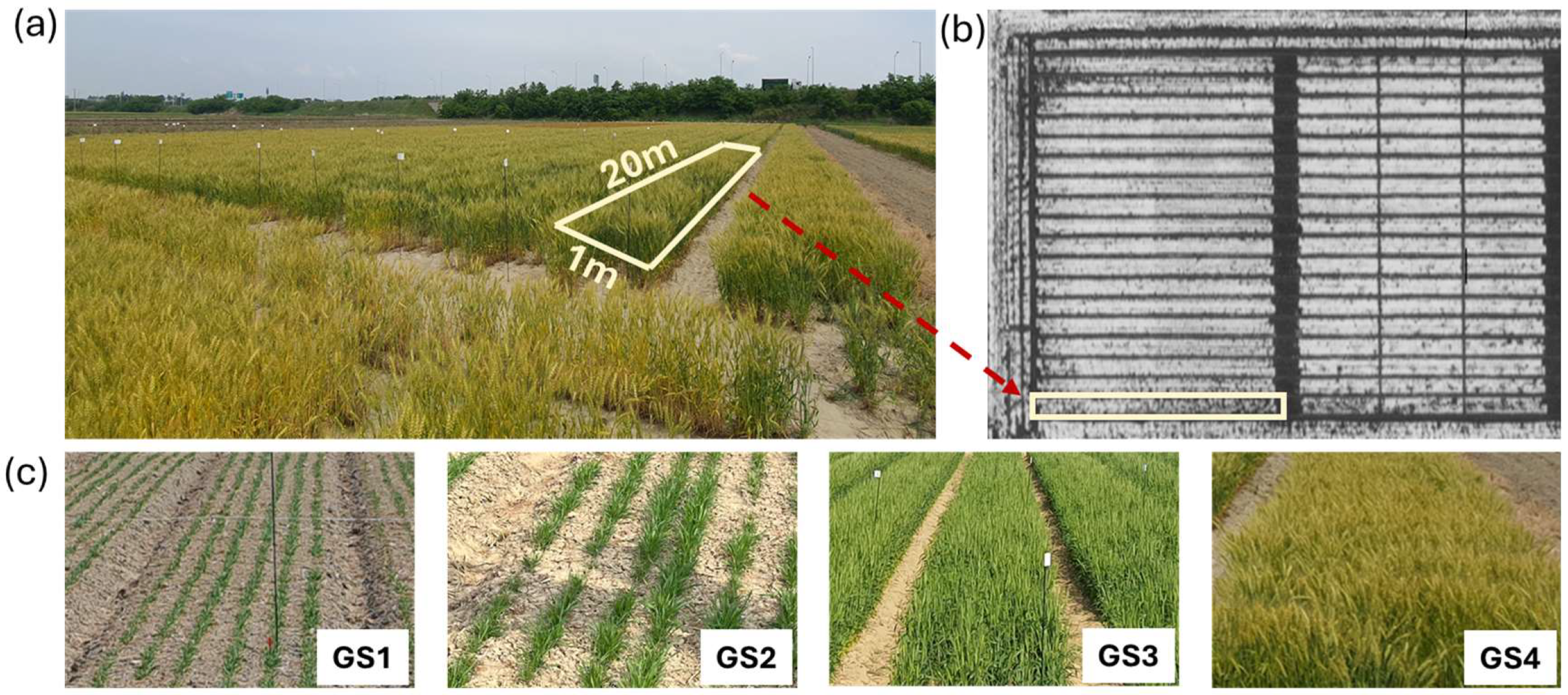
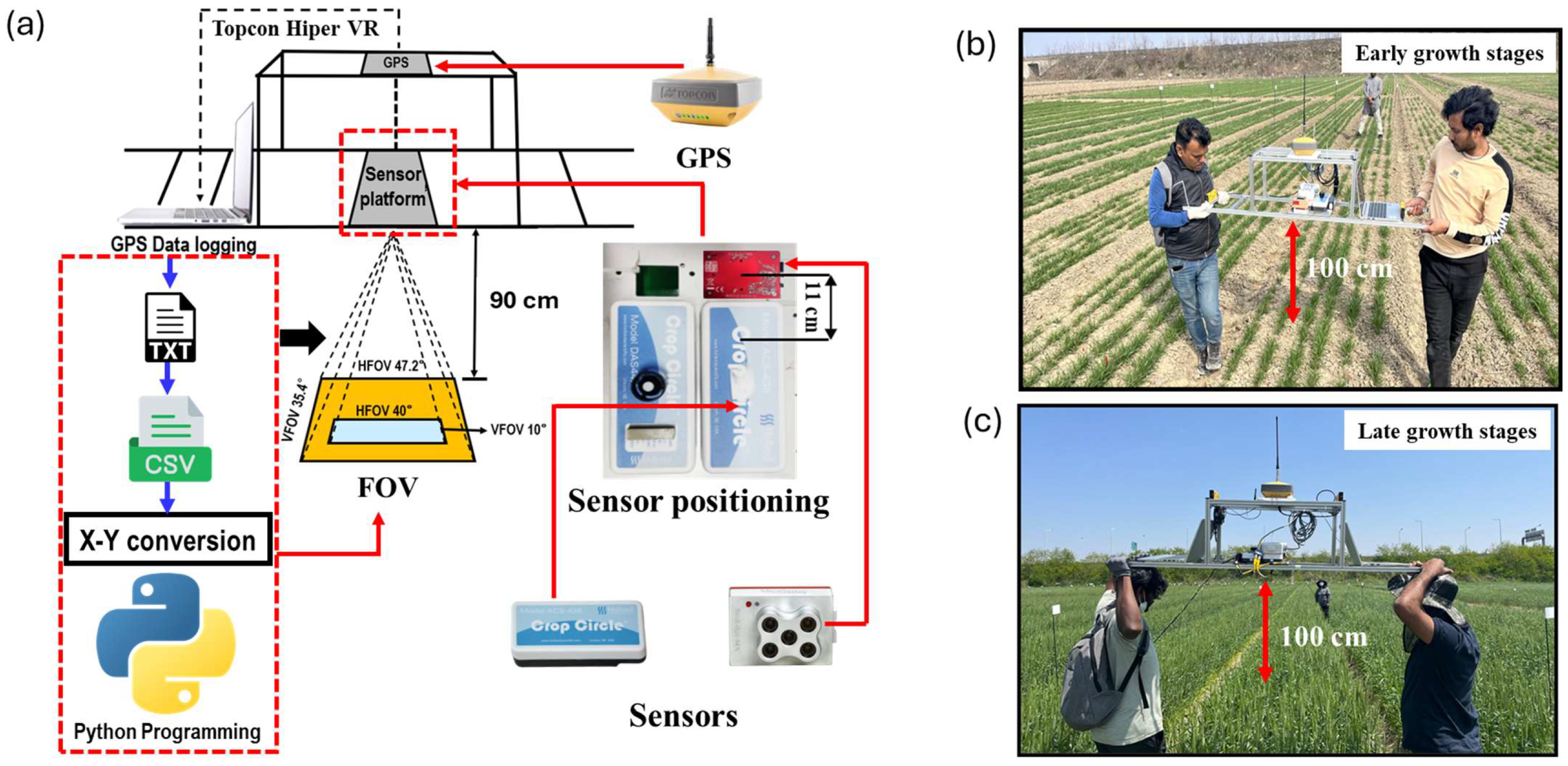
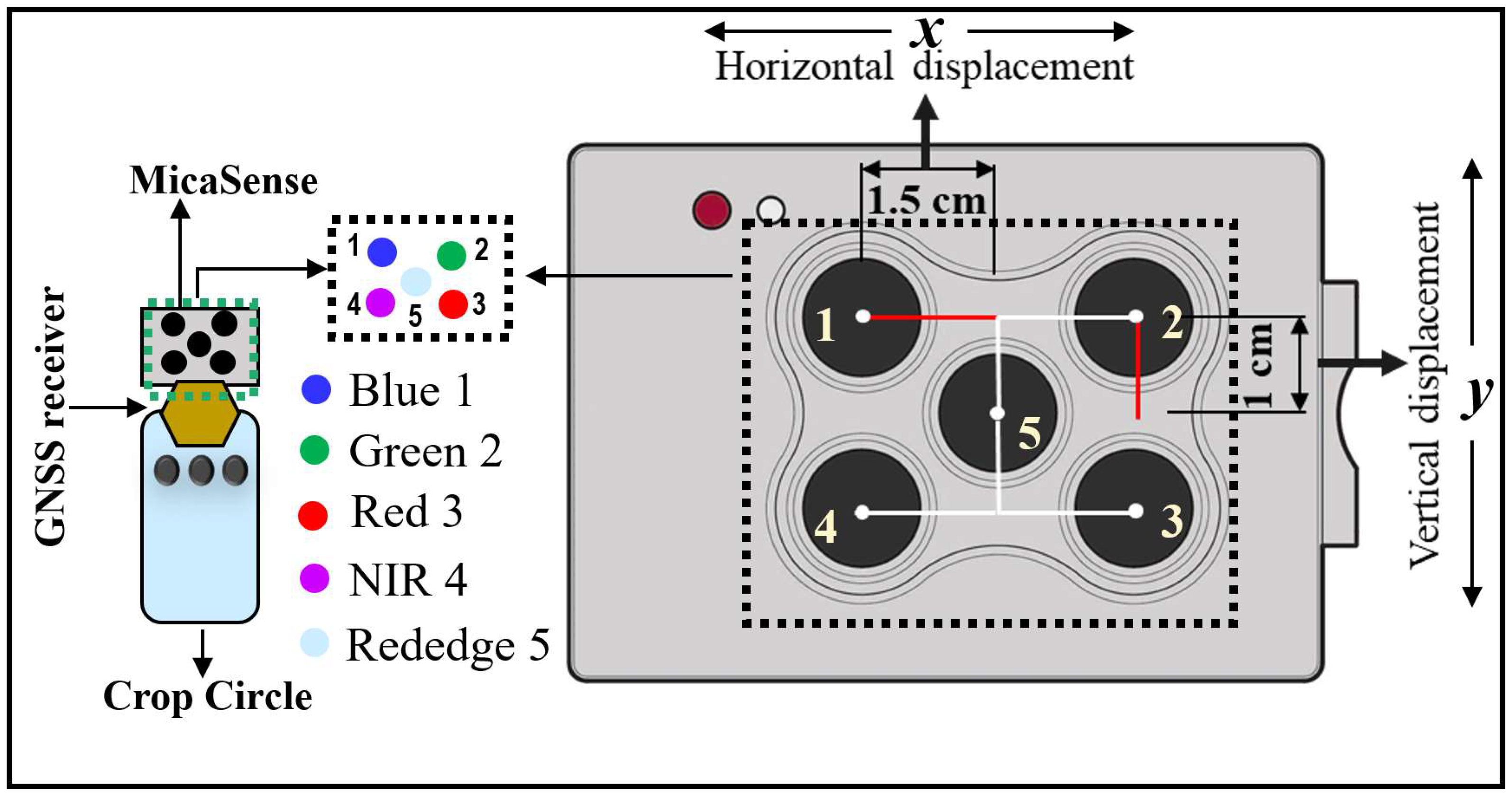
2.1. Study Area, Sensors, and Data Collection

The study was conducted in a wheat field located at National Institute of Agricultural Sciences, Rural Development Administration, Jeonju, Republic of Korea (Latitude 35°52′49.65″N, Longitude 127°2′39.95″E), as shown in Figure 1a. From the wheat field, an experimental plot was selected with a dimension of 1 m wide and 20 m long (Figure 1b). The wheat crop plot was used to ensure accurate and manageable data collection while facilitating a meaningful analysis of the wheat crop growth under the optimum conditions. The study was conducted over three months, spanning from March to May, which corresponds to four key growth stages (GS) of wheat, namely tillering (GS1), stem elongation (GS2), heading (GS3), and grain filling (GS4), as shown in Figure 1c. To ensure data reliability and representativeness, a random sampling method was implemented. Three datasets were collected from each section of the experimental plot, and the average values were used to enhance measurement accuracy. Sampling points were selected randomly to avoid biased measurements, ensuring that the results were reflective of general sensor performance rather than specific spatial variations within the plot.

In this study, the primary objective was to evaluate the data enhancement technique for multispectral imagery. To achieve this, two widely recognized commercial multispectral sensors were used: a passive sensor (MicaSense RedEdge MX, AgEagle Aerial Systems Inc., Wichita, KS, USA) and an active sensor (Crop Circle ACS-435; Holland Scientific Inc., Lincoln, NE, USA). The specifications of these sensors are mentioned in

Table 1. Specifications of the sensors applied during the experiment.

Item	Passive Multispectral Sensor	Active Reflectometry Sensor
Model	MicaSense RedEdge MX	Crop Circle ACS-435
Sensor type	Passive sensor	Active sensor
Dimensions (m)	0.121 × 0.066 × 0.046	0.038 × 0.178 × 0.076
Weight	150 g	385 g
Sensing interval	1 s	1–10 s
Center wavelength	Blue (475), Green (560), Red (668), NIR (717), RedEdge (840)	Red (670), NIR (717), RedEdge (730)
Resolution	1280 × 960 pixels
Focal length	5.4 mm
FOV	47.2° (HFOV), 35.4° (VFOV)	40~45° (HFOV), 6~10° (VFOV)
Ground sampling distance @ 60 m Ground sampling distance @ 3 m	~4 cm/pixel per band ~2.5 mm/pixel per band

. These sensors were chosen for their extensive application in agricultural research where they are known for their reliability and accuracy in capturing vital crop and vegetation data. The passive sensor is a state-of-the-art sensor capturing five narrow spectral bands, which are essential for a detailed analysis of plant health and vigor. On the other hand, the active sensor is renowned for the robust performance in field conditions and the ability to provide consistent data across large agricultural areas.

The effectiveness of these sensors was evaluated using the NDVI, a widely accepted and standard metric for assessing plant health based on the difference between near-infrared and red light [46,47,48]. NDVI is a crucial indicator in agricultural research, as it provides insights into crop conditions, allowing for early detection of stress, disease, or other factors that might impact yield [49].

Table 2. Different growth stages of wheat for this study.

Growth Stage	Data Collection Date	Days After Sowing	Data Collection Start Time	Data Collection End Time
GS1	20 March 2023	10	14:38	15:01
GS2	14 April 2023	34	14:46	15:10
GS3	10 May 2023	70	15:01	15:26
GS4	24 May 2023	84	14:54	15:18

presents detailed information regarding the wheat growth stages, along with the specific sowing dates for the study. To facilitate accurate and consistent data collection, an aluminum profile structure was prepared to mount both the active and passive sensors side by side along with a real-time kinematics (RTK) GNSS receiver (Hiper VR, Topcon Positioning Systems Inc., Livermore, CA, USA). The RTK GNSS receiver used in this study has a horizontal accuracy of 5 mm + 0.5 ppm and a vertical accuracy of 10 mm + 0.8 ppm. This advanced RTK GNSS receiver was included to extract precise timestamps, ensuring that sample points from different sensors were accurately matched based on time synchronization. This setup ensured that both sensors could simultaneously capture data from the field under identical conditions, maintaining uniformity in positioning and timing, as illustrated in Figure 2. The sensor height was selected based on a 1 m ridge width to ensure optimal horizontal FOV coverage and maximize data acquisition consistency, as illustrated in Figure 2.

To ensure the reliability and validity of the enhancement method, data collection at four key growth stages of the wheat crop was performed. Data were collected from a total of 77 random sample points matched with the timestamp data within the designated plot, allowing for a comprehensive assessment of the condition of the wheat crops and the effectiveness of the sensors throughout the growing season. During the data collection, the calibration procedures were conducted on the multispectral sensor, including radiometric and dynamic light scattering (DLS) calibration. Radiometric calibration was performed before and after each data acquisition session to ensure accurate and consistent multispectral data. Additionally, DLS calibration was conducted prior to data collection, crucially accounting for ambient lighting variations and enabling precise reflectance value extraction from the imagery. These calibrations were essential for ensuring the accuracy and consistency of the sensor in capturing multispectral data.

To address potential errors associated with data collection procedure by different personnel at different times, we implemented standardized positioning techniques to ensure consistency. If the height of the data collector was the same, both individuals maintained the same holding position (e.g., above the head, Figure 2c). In cases where personnel had different heights, a fixed reference point on the body (e.g., chest or abdomen, Figure 2b) was used to maintain a uniform sensor height (100 cm from the crop canopy). This approach minimized altitude and tilt discrepancies. Additionally, controlled handling techniques were employed to reduce sensor shaking during data acquisition. This approach was specifically designed to reduce potential variations caused by changes in sun angle, human shadows, and fluctuations in light intensity throughout the data collection process. These measures were taken to ensure that the procedural variations had minimal impact on the accuracy and consistency of the collected data. Data collection was carefully synchronized to maintain consistent timing across all measurements. Recognizing the importance of minimizing these variables, the aim was to ensure that the data gathered reflected true differences in the field rather than artifacts of the measurement process. A key challenge was to align the FOV of the active and passive sensors to avoid inconsistencies in data collection. To fulfill the objective of achieving precise FOV alignment, data collection ensures accurate and comparable multispectral imagery. The experimental design focused on evaluating the enhancement technique: FOV alignment to harmonize sensor data. This method was tested to quantify the effectiveness and contribution to more accurate multispectral data processing.

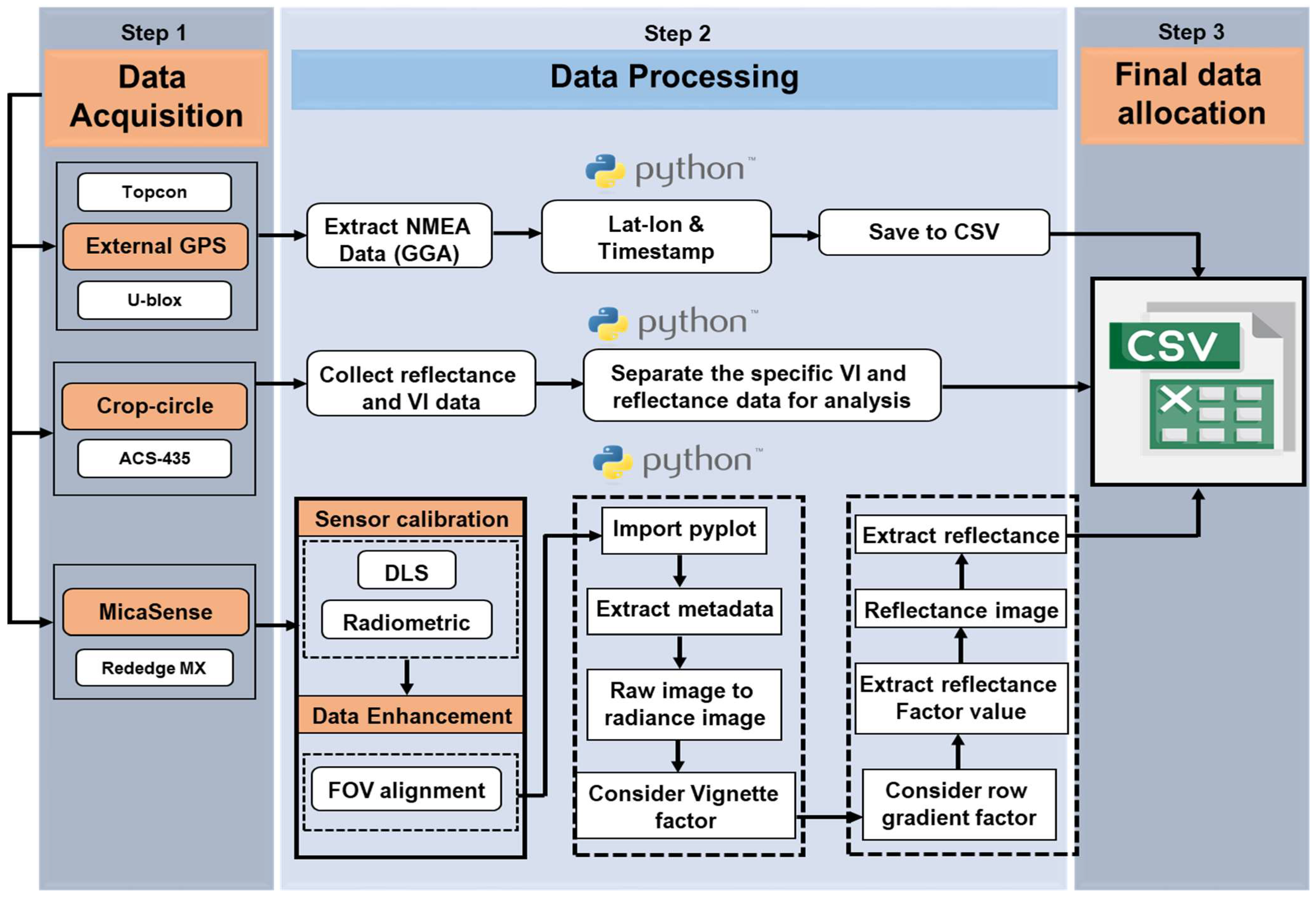
2.2. Multispectral Data Processing Procedures

Multispectral data were collected from the wheat field at four key growth stages using both active and passive sensors. Data from the active sensor was processed in a spreadsheet (Microsoft Excel 2016, Microsoft, Redmond, WA, USA), which provided tools for data organization, statistical analysis, and visualization. Specific functions, such as the data analysis tool pack for descriptive statistics and regression analysis. While the multispectral data from passive sensor underwent calibration to generate radiometrically accurate images across multiple spectral bands. This multi-step calibration and vignette correction process converted raw digital values into radiance values (L), measured in Wm⁻²sr⁻¹nm⁻¹, enabling precise quantitative analysis.

The initial raw digital values from the multispectral images required conversion to radiance using a manufacturer-provided calibration equation (Equation (1)) [50], which incorporated sensor-specific radiometric coefficients and image acquisition parameters. This systematic approach ensured a reliable spectral analysis and consistency across different growth stages, facilitating an accurate comparison of data as follows:

$$\mathrm{L}=\mathrm{V}\left(\mathrm{x},\mathrm{y}\right)\times {\displaystyle \frac{{\mathrm{a}}_1}{\mathrm{g}}}\times {\displaystyle \frac{\mathrm{p}-{\mathsf{\rho }}_{\mathrm{B}\mathrm{L}}}{{\mathrm{t}}_{\mathrm{e}}+{\mathrm{a}}_2\mathrm{y}-{\mathrm{a}}_3{\mathrm{t}}_{\mathrm{e}}\mathrm{y}}}$$

(1)

where L is the radiance in Wm⁻²sr⁻¹nm⁻¹, V(x, y) is the vignette polynomial function for pixel location (x, y), a₁, a₂, and a₃ are the radiometric calibration coefficients, g is the sensor gain setting, p is the normalized raw pixel value (divided by 2N, where N is the number of bits in the images), x and y are the pixel row and column numbers, ${\mathsf{\rho }}_{\mathrm{B}\mathrm{L}}$ is the normalized black-level value, and te is the image exposure time in millisecond (ms).

The multispectral images often exhibit vignette effects due to the lens configuration, where pixels farther from the center receive less light. A radial vignette model corrects this effect, ensuring uniform radiance across the field of view by compensating for light sensitivity discrepancies. Using the multispectral Python package [51], the raw images were transformed into radiance data. A radial vignette model was applied to correct the fall of light sensitivity in pixels located further from the center of the image. To apply the radial vignette correlation for the intensity of each pixel in the multispectral images, a systematic approach using the provided image metadata was followed. The process is mathematically defined using Equations (2)–(4) as follows [52]:

$$\mathrm{r}=\sqrt{{(\mathrm{x}-{\mathrm{c}}_{\mathrm{x}})}^2+{(\mathrm{y}-{\mathrm{c}}_{\mathrm{y}})}^2}$$

(2)

$$\mathrm{k}=1+{\mathrm{k}}_0\times \mathrm{r}+{\mathrm{k}}_1\times {\mathrm{r}}^2+{\mathrm{k}}_2\times {\mathrm{r}}^3+{\mathrm{k}}_3\times {\mathrm{r}}^4+{\mathrm{k}}_4\times {\mathrm{r}}^5+{\mathrm{k}}_5\times {\mathrm{r}}^6$$

(3)

$${\mathrm{I}}_{\mathrm{c}\mathrm{o}\mathrm{r}\mathrm{r}\mathrm{e}\mathrm{c}\mathrm{t}\mathrm{e}\mathrm{d}}(\mathrm{x},\mathrm{y})={\displaystyle \frac{\mathrm{I}(\mathrm{x},\mathrm{y})}{\mathrm{k}}}$$

(4)

where r is the distance of the pixel (x, y) from the vignette center in pixels, (x, y) is the coordinate of the pixel being corrected, k is the correction factor by which the raw pixel values are divided to correct for vignette, I (x, y) is the original intensity of pixel at x, y, I_corrected (x, y) is the corrected intensity of pixel at x, y, and in Equation 1, V (x, y) is equal to 1/k.

The data acquisition time was synchronized with the data obtained from the GNSS receiver, facilitating precise georeferencing. The sensors were consistently maintained at a height of ~100 cm to encompass the FOV along the horizontal axis (width) of the study plot. The height was determined based on the plot width. Although the plot measured 1 m in width, the wheat was planted within an 80 cm span. Therefore, Equation (5) was applied, using the wheat width (W_H) of 80 cm, to calculate the height required for the sensors to cover the entire plot. Additionally, a uniform data acquisition speed of 0.23 ms⁻¹ was maintained throughout the process, further enhancing the accuracy and consistency of the collected data. In the data post-processing phase, the Python programming language and geographic information system (GIS) software (QGIS 3.32, QGIS Development Team, Available at: https://www.qgis.org; accessed on 23 September 2024) were used for the comprehensive processing and analysis of multispectral data, facilitating the extraction of valuable insights through advanced geospatial processing and image analysis techniques. The data from the active sensor was stored directly in an Excel data sheet for further analysis. The integration of these detailed data acquisition, calibration, and processing procedures ensured the robustness of the research outcomes.

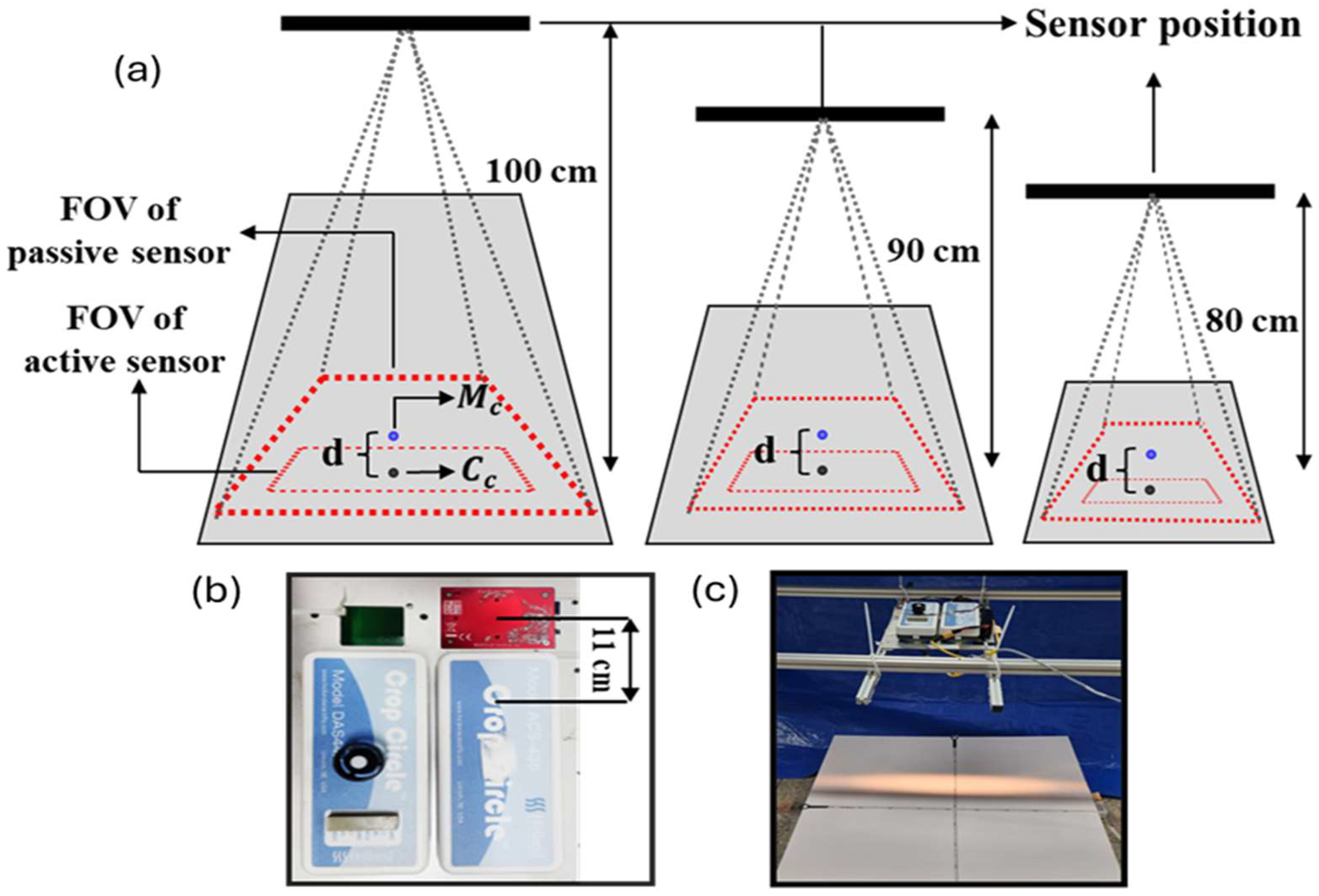
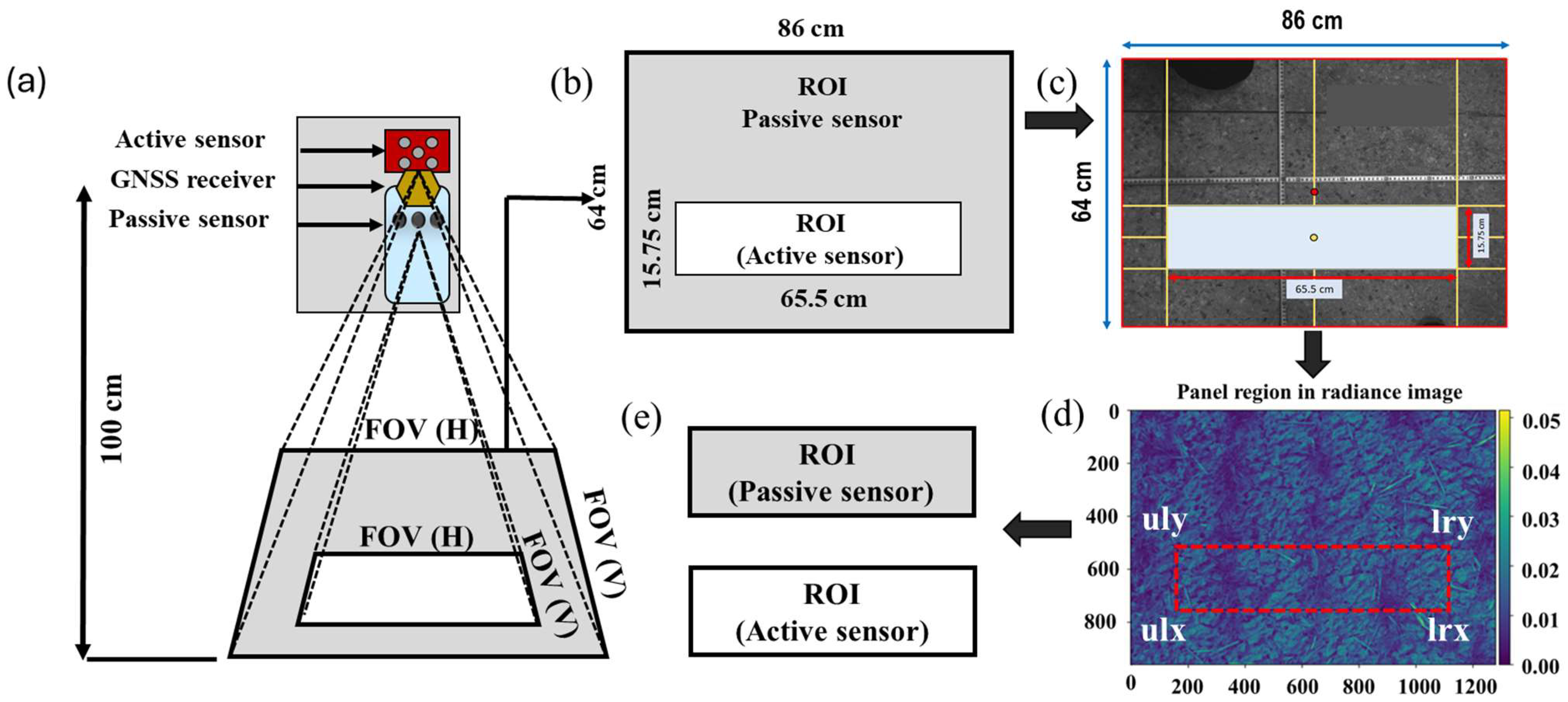
2.3. FOV Alignment Procedure

A comprehensive laboratory experiment was conducted to standardize the FOV alignment between the passive and active sensors. This experiment addressed the discrepancies in the center point positioning of the two sensors, which potentially impacted the accuracy and reliability of the data collected. To achieve precise alignment, both sensors were mounted on a robust aluminum structure designed specifically for field data collection. This setup facilitated the precise positioning and adjustment of the sensors, ensuring consistent measurements across varying conditions. To cover the designated region of interest (ROI) with the FOV of the active sensor, three canopy heights were selected: 80, 90, and 100 cm (Figure 3a). The active sensor continuously maintained the ROI’s center at a fixed distance, ensuring a consistent area across all heights. However, the image dimension length (L) and width (W) varied depending on the sensor height. Meanwhile, the sensors were positioned at a minimum feasible distance of 11 cm to ensure proper alignment and maintain FOV consistency between the active and passive sensors (Figure 3b). Increasing the distance beyond this threshold could have led to partial misalignment, potentially affecting data accuracy and consistency in multispectral measurements. This measurement was confirmed using a measuring tape aligned with the projection of both sensors’ center points, ensuring accuracy. This setup as shown in Figure 3c effectively addressed FOV discrepancies, enabling reliable data collection across different heights.

The methodology for aligning the field of view (FOV) between the active and passive sensors was carried out in a stepwise manner to ensure accuracy and reproducibility. Initially, the dimensions of a single pixel were determined by dividing the image’s total length and width by using resolution in the horizontal and vertical directions, respectively. This calculation was essential as it provided the foundational measurements required for subsequent geometric alignment. Equations (5) and (6) were applied to calculate the pixel width and height, ensuring precision in determining the physical size of each pixel within the image frame [53].

$${\mathrm{P}}_{\mathrm{w}}={\displaystyle \frac{2\times \mathrm{h}\times \mathrm{t}\mathrm{a}\mathrm{n}\left(\frac{{\mathsf{\theta }}_{\mathrm{H}}}{2}\right)}{{\mathrm{R}}_{\mathrm{H}}}}$$

(5)

$${\mathrm{P}}_{\mathrm{l}}={\displaystyle \frac{2\times \mathrm{h}\times \mathrm{t}\mathrm{a}\mathrm{n}\left(\frac{{\mathsf{\theta }}_{\mathrm{V}}}{2}\right)}{{\mathrm{R}}_{\mathrm{V}}}}$$

(6)

where P_w and P_l are the pixel width and length of the image, respectively, and R_H and R_V are the horizontal and vertical resolutions of the image in pixels.

With the pixel dimensions established, the reference center point of the passive sensor (MicaSense) was identified within the image resolution. The specific pixel corresponding to this center point was located based on the sensor’s placement and its known alignment with the imaging structure. This reference point served as the starting position for aligning the active sensor (Crop Circle). The displacement between the two sensor centers was defined as 11 cm (Figure 3b), a value verified through experiments that demonstrated consistency across various heights. Since the displacement occurred along the vertical axis, the horizontal coordinate remained unchanged, and only the vertical coordinate was adjusted. Using the pixel size determined earlier, the 11 cm displacement was converted into the corresponding pixel count using Equation (6). This conversion enabled the precise identification of the active sensor’s center pixel within the image frame.

To further refine the analysis, Equations (7) and (8) were introduced to compute the pixel count for specific distances along both the x-axis (dx) and y-axis (dy), representing the spatial extent in the horizontal and vertical directions, respectively. These pixel counts were derived from the distance between the sensors mounted on the aluminum structure, which was crucial in synchronizing the sensor outputs. The value of dy was particularly emphasized since the sensors were mounted along the y-axis, and vertical alignment played a critical role in ensuring uniformity in data acquisition. Once the pixel count for the 11 cm distance between the passive and active sensors was determined using Equation 8, the vertical configuration of the sensors allowed all key parameters to be focused on the y-axis.

$${\displaystyle \frac{{\mathrm{d}}_{\mathrm{x}}}{{\mathrm{P}}_{\mathrm{w}}}}={\displaystyle \frac{2\times \mathrm{h}\times \mathrm{t}\mathrm{a}\mathrm{n}\left(\frac{{\mathsf{\theta }}_{\mathrm{H}}}{2}\right)}{{\mathrm{R}}_{\mathrm{H}}}}$$

(7)

$${\displaystyle \frac{{\mathrm{d}}_{\mathrm{y}}}{{\mathrm{P}}_{\mathrm{l}}}}={\displaystyle \frac{2\times \mathrm{h}\times \mathrm{t}\mathrm{a}\mathrm{n}\left(\frac{{\mathsf{\theta }}_{\mathrm{V}}}{2}\right)}{{\mathrm{R}}_{\mathrm{V}}}}$$

(8)

where ${\mathrm{d}}_{\mathrm{x}}$ and ${\mathrm{d}}_{\mathrm{y}}$ are any distances towards the x-axis and y-axis, respectively, among the sensors and within the projection of the image, ${\mathrm{P}}_{\mathrm{w}}$ and ${\mathrm{P}}_{\mathrm{l}}$ are the length and width of a single pixel, h is the height of the sensor measured from the canopy, ${\mathsf{\theta }}_{\mathrm{H}}$ and ${\mathsf{\theta }}_{\mathrm{V}}$ are the horizontal field of view (HFOV) and Vertical field of view (VFOV), ${\mathrm{R}}_{\mathrm{H}}$ is the resolution of the image in horizontal direction, and ${\mathrm{R}}_{\mathrm{V}}$ represents resolution of the image in the vertical direction.

The field of view (FOV) for the active sensor was then calculated to determine the extent of its coverage in both the horizontal and vertical directions. Equations (9) and (10) (Holland Scientific, Lincoln, NE, USA) were employed to compute the horizontal and vertical FOV values. To simplify subsequent calculations, these FOV measurements were halved, representing the distances from the sensor’s center to the outer edges of its field. The half-distances were then converted into pixel counts using the established pixel dimensions, providing the necessary parameters to define the FOV boundaries within the image.

$${\mathrm{W}}_{\mathrm{H}}=2\times \mathrm{h}\times \mathrm{t}\mathrm{a}\mathrm{n}\left({\displaystyle \frac{{\mathsf{\theta }}_{\mathrm{H}}}{2}}\right)$$

(9)

$${\mathrm{W}}_{\mathrm{V}}=2\times \mathrm{h}\times \mathrm{t}\mathrm{a}\mathrm{n}\left({\displaystyle \frac{{\mathsf{\theta }}_{\mathrm{V}}}{2}}\right)$$

(10)

where W_H and W_V are the horizontal and vertical FOVs, respectively, h is the height of the sensor above the canopy, and θ_H and θ_V are the horizontal and vertical angles of view.

For the active sensor, the four corner points of the FOV were calculated relative to its center pixel. Starting from the center, adjustments were made in the horizontal and vertical directions to locate each corner. For example, the lower-right corner was determined by increasing the horizontal coordinate by the pixel count corresponding to half the horizontal FOV and decreasing the vertical coordinate by the pixel count representing half the vertical FOV. This process was repeated for the other corners, with appropriate directional adjustments made for each. The coordinates for these corner points were subsequently used in data extraction processes to identify reflectance values within the defined region. This process enabled the accurate measurement of the common ROI between the two sensors, as illustrated in Figure 4. To determine the pixel coordinates of the four corners within the common FOV, the pixel count method was employed. Using Equations (7) and (8), this method calculated the pixel offset from the center coordinate (Cc) to locate each corner: the upper left x-coordinate (ulx), upper left y-coordinate (uly), lower right x-coordinate (lrx), and lower right y-coordinate (lry), as illustrated in Figure 4d.

In addition to sensor-to-sensor alignment, intra-sensor geometric alignment was performed for the passive sensor, which contained multiple lenses. The relative displacements of these lenses from the central lens accounted for using their fixed physical offsets. The known displacements along the x- and y-axes (Figure 5) were converted into pixel counts based on the previously calculated pixel dimensions. Using the same methodology as described for the active sensor, the corner coordinates for the FOV of each lens were determined. Each lens’s FOV was treated independently, ensuring that the reflectance values for individual bands were extracted with high precision. Then, to extract from the common ROI of the images, the Python OpenCV library was employed. Afterwards, The OpenCV function cv2.rectangle() was utilized to mark the specified ROI for extracting reflectance. Figure 4d. These coordinates were extracted for a single image (RedEdge) Figure 4e. In our search, the ‘msutils’ module was used to extract the reflectance values from the chosen ROI. This procedure allowed the FOV of the active sensor to be aligned with the center point of passive sensor, specifically within the center image (RedEdge). Considering the distortion, individual coordinate sets (ulx, uly, lrx, and Iry) for each lens were extracted for each individual image. These coordinates were subsequently marked on the multispectral image using the same Python programming language code to measure the area of the active sensor. For further calculation, the ROI of Red and NIR were marked using those coordinates to extract the reflectance values. Equation (11) was introduced to calculate the NDVI using those reflectance to assess the accuracy of this technique [54]. The NDVI values from raw images were also calculated using the Python programming language. These raw data were applied to evaluate the percentage of enhancement using the FOV alignment technique.

$$\mathrm{N}\mathrm{D}\mathrm{V}\mathrm{I}={\displaystyle \frac{{\mathsf{\rho }}_{\mathrm{n}\mathrm{i}\mathrm{r}}-{\mathsf{\rho }}_{\mathrm{r}\mathrm{e}\mathrm{d}}}{{\mathsf{\rho }}_{\mathrm{n}\mathrm{i}\mathrm{r}}+{\mathsf{\rho }}_{\mathrm{r}\mathrm{e}\mathrm{d}}}}$$

(11)

where ${\mathsf{\rho }}_{\mathrm{n}\mathrm{i}\mathrm{r}}$ and ${\mathsf{\rho }}_{\mathrm{n}\mathrm{i}\mathrm{r}}$ are considered as the reflectance of NIR and red bands, respectively.

This methodology focused not only on the alignment between the active and passive sensors but also on the internal alignment of multiple lenses within the passive sensor. The approach ensured accurate geometric calibration across all lenses and sensors, enabling the precise extraction of reflectance data for subsequent analysis. The method is flexible and can be adapted for use with other sensors, provided the height and lens-to-lens displacements are known. Furthermore, the consistency of the center-to-center distance between sensors, irrespective of height, underscores the robustness of this approach for FOV alignment in multispectral imaging applications. By integrating these calculations into the data processing workflow, a comprehensive framework for sensor alignment was established, offering a reliable solution for multispectral sensor geometric calibration.

Reflectance values were extracted from the multispectral image bands using Python, with NumPy facilitating array manipulation. These extracted reflectance values were saved in an Excel file for NDVI computation using Equation (11). Subsequently, the QGIS software package was utilized to extract NDVI data from clipped images following FOV alignment, enabling a direct evaluation of NDVI values derived from Python-based processing against spatially analyzed outputs. This integration ensured consistency and validated the NDVI results within the geospatial framework. This streamlined approach ensured the reproducibility of results while optimizing the data processing pipeline for agricultural applications.

For the total workflow of this study, and to minimize potential variability errors and ensure the accuracy of NDVI measurements, several methodological measures were implemented. First, precise data extraction was conducted within fixed regions of interest (ROIs) across all spectral bands to standardize the data processing workflow and enhance comparability. The alignment of the field-of-view (FOV) with the active sensor was performed using a predefined geometric calibration method, thus reducing spatial distortions and improving measurement accuracy. Furthermore, background interference from non-vegetative elements was minimized by ensuring data extraction from centrally located ROIs, where edge distortions were least pronounced. In addition, intra-sensor geometric alignment was applied to correct minor misalignments among spectral bands by translating physical displacements into pixel coordinates. These measures collectively contributed to improved consistency in data collection and reduced potential sources of variability, strengthening the reliability of the experimental results.

A comprehensive statistical analysis was conducted to elucidate the relationships within the dataset saved in the Excel data sheet (Figure 6), focusing on four distinct growth stages of rice cultivation. This analysis aimed to identify underlying patterns and provide meaningful insights into the dynamics of the data. To assess the relationships between various parameters, a coefficient correlation heatmap was employed. This visualization technique facilitated a clear representation of how each variable interacts with others across the growth stages. The Pearson correlation coefficient (r) was calculated using Equation (12).

$$\mathrm{r}={\displaystyle \frac{\mathrm{n}(\sum \mathrm{x}\mathrm{y})-(\sum \mathrm{x}\left)\right(\sum \mathrm{y})}{\sqrt{[\mathrm{n}\sum {\mathrm{x}}^2-{\left(\sum \mathrm{x}\right)}^2\left]\right[\mathrm{n}\sum {\mathrm{y}}^2-{\left(\sum \mathrm{y}\right)}^2]}}}$$

(12)

where n is the number of paired observations, and x and y are the variables that need to be correlated.

The heatmap provides a visual interpretation of these correlations, highlighting strong, weak, and negative relationships. This step is crucial for understanding the interactions among variables, which can inform subsequent analyses and interpretations. Following the correlation analysis, regression techniques were applied to quantify the relationships further and predict outcomes based on the observed data. The regression model facilitates the understanding of how different variables influence each other, enabling the development of predictive insights relevant to rice growth. In addition to correlation and regression analyses, violin charts were utilized to illustrate the distribution of data across different growth stages. Violin plots combine the benefits of box plots and density plots, providing a detailed view of the data distribution while revealing underlying patterns. This visualization aids in identifying trends and anomalies in the dataset. To evaluate the accuracy of the regression model and its predictions, the root mean square error (RMSE) was calculated. The RMSE is a widely used metric that quantifies the difference between predicted and observed values, providing a clear indication of model performance. It is calculated using Equation (13) as follows:

$$\mathrm{R}\mathrm{M}\mathrm{S}\mathrm{E}=\sqrt{\sum _{\mathrm{i}=1}^{\mathrm{n}}{\displaystyle \frac{{(\widehat{{\mathrm{y}}_{\mathrm{i}}}-{\mathrm{y}}_{\mathrm{i}})}^2}{\mathrm{n}}}}$$

(13)

where ${\widehat{y}}_i$ is the predicted value, $y_i$ is the observed value, and n is the number of observations.

3. Results

In this study, precise data extraction from individual images within specific ROIs was essential for the accurate and reliable calculation of VIs from multispectral sensors. Figure 7 presents the ROIs in multispectral images after the alignment of FOV with the active sensor, highlighted by red rectangles, selected across five spectral bands. These ROIs were consistently applied to all images collected in the wheat field to standardize the data processing workflow. The uniform selection of ROIs ensured comparability across bands, enhancing the accuracy of VIs by minimizing potential variability due to image alignment or distortion. This approach enabled the precise tracking of plant health metrics across spectral bands, facilitating improved assessment of crop conditions.

Across all five spectral bands, a small but notable distortion in the pixel coordinates of the red-marked regions was observed as shown in Figure 7, reflecting slight variations in alignment among the sensor lenses. The dimensions of a single pixel in the image were calculated. Using the known image resolution (1260 × 980 pixels) and the physical dimensions of the image (86 cm × 64 cm), the width and height of each pixel were found to be approximately 0.065 cm × 0.065 cm. This step provided the fundamental measurements necessary for pixel-based calculations across the entire image, forming the basis for determining sensor and lens alignments. The central pixel of the passive sensor (MicaSense) was identified at coordinates (630, 490) within the image resolution. This center served as the reference point for subsequent calculations, enabling the alignment of the active sensor (Crop Circle) relative to the passive sensor. The center-to-center distance between the sensors was determined experimentally to be a constant 11 cm, regardless of the height of the imaging system. By translating this physical displacement into a vertical pixel count, it was calculated that the 11 cm displacement corresponded to 168 pixels. Consequently, the center pixel for the active sensor was identified at coordinates (630, 658), with the x-coordinate remaining unchanged and the y-coordinate adjusted by the calculated pixel count. The horizontal and vertical FOV (HFOV and VFOV) of the active sensor were then determined using the established equations. The HFOV and VFOV were measured as 65.4 cm and 15.75 cm, respectively. To define the boundaries of the FOV, half of these values were used, corresponding to 32.7 cm (half HFOV) and 7.875 cm (half VFOV). These distances were converted into pixel counts, resulting in 503 pixels for the half HFOV and 121 pixels for the half VFOV. Using these values, the four corner points of the FOV for the active sensor were calculated relative to its center pixel at (630, 658).

For the lower-right corner, 503 pixels were added to the x-coordinate, and 121 pixels were subtracted from the y-coordinate, resulting in a pixel location of (1133, 537). Similarly, the lower-left corner was located at (1133, 779), the upper-right corner at (127, 537), and the upper-left corner at (127, 779). To create the bounding box for the required ROI, y values from upper left corner (uly) and upper right corner (lry) and x values from lower left corner (ulx) and lower right corner (lrx) were taken. Finally, the coordinates for aligned image was calculated (uly, ulx, lry, lrx: 537, 127, 537, 1133). These corner coordinates defined the active sensor’s FOV within the image, allowing the precise extraction of reflectance data from the corresponding region.

The passive sensor, equipped with multiple lenses, required additional intra-sensor geometric alignment. The relative displacements of the lenses from the central lens were identified as 1.5 cm along the x-axis and 1 cm along the y-axis. These displacements were translated into pixel counts, corresponding to 23 pixels horizontally and 15 pixels vertically, respectively. For each lens, the corner points of its FOV were calculated using the same methodology applied to the active sensor. This step ensured that the reflectance data from all lenses, each representing a distinct spectral band, were accurately aligned and extracted.

Table 3. Final coordinates for each band image to extract reflectance maintaining the FOV alignment.

Band Images	uly	ulx	lry	lrx
1	522	104	522	1110
2	522	150	522	1156
3	552	150	552	1156
4	552	104	552	1110
5	537	127	537	1133

illustrates the final coordinates for all the band images, emphasizing the importance of these coordinates for sensor alignment to ensure accurate reflectance extraction from precisely aligned sensors.

The combined results illustrate both sensor-to-sensor alignment and intra-sensor alignment. By integrating the corner coordinates of all lenses and sensors into the data processing workflow, the geometric calibration ensured precise alignment across the multispectral imaging system. Additionally, the method’s adaptability for different sensor heights and configurations was confirmed, as the pixel dimensions and alignments were consistently maintained across varying experimental setups. These results highlight the robustness of the alignment methodology and its potential as a reliable alternative for multispectral sensor geometric calibration. The accurate determination of pixel dimensions, center points, and FOV boundaries ensures that reflectance values are precisely extracted, contributing to improved reliability and precision in multispectral imaging and analysis.

These subtle variations in pixel coordinates are likely caused by minor misalignments between the individual lenses of the multispectral camera system. To counteract potential distortions or edge artifacts, the red-marked regions were carefully chosen to be centered within the image, as the central part was less susceptible to the edge distortions that can arise from lens aberrations or misalignment. By focusing on the central portion of each image, more reliable and undistorted pixel data across all bands were captured, improving the accuracy of the extracted reflectance values. This ensures that any VI calculations, such as NDVI, are based on high-quality data, minimizing errors introduced by peripheral distortions.

Although the extraction coordinates were fixed, due to manual handling, small distortions caused by height fluctuation could be found. The distortion data show that consistent shifts were observed across the bands for each spatial region, but with slight variations in magnitude (Figure 8). During the analysis, pixel coordinates from Band 1 were used as reference points to assess distortions in the other bands. At the reference pixel (1085, 338) in Band 1, shifts were observed in the x and y axes: (35, 12) pixels, (38, −25), (−17, −28), and (8, −11) for Bands 2, 3, 4, and 5, respectively (Figure 8). Similar distortions were detected at another reference point, (581, 642), where the shifts measured (36, 11), (35, −23), (−17, −31), and (9, −13) for Bands 2, 3, 4, and 5, respectively. These consistent spatial shifts across different coordinates provided a basis for correcting alignment discrepancies between the bands. These variations indicated that while there is a general alignment between the images, slight misalignments in both the x and y directions are consistent across the bands. The calculated shifts can be corrected during data processing, especially for NDVI or other vegetation index calculations that rely on pixel-to-pixel alignment across bands.

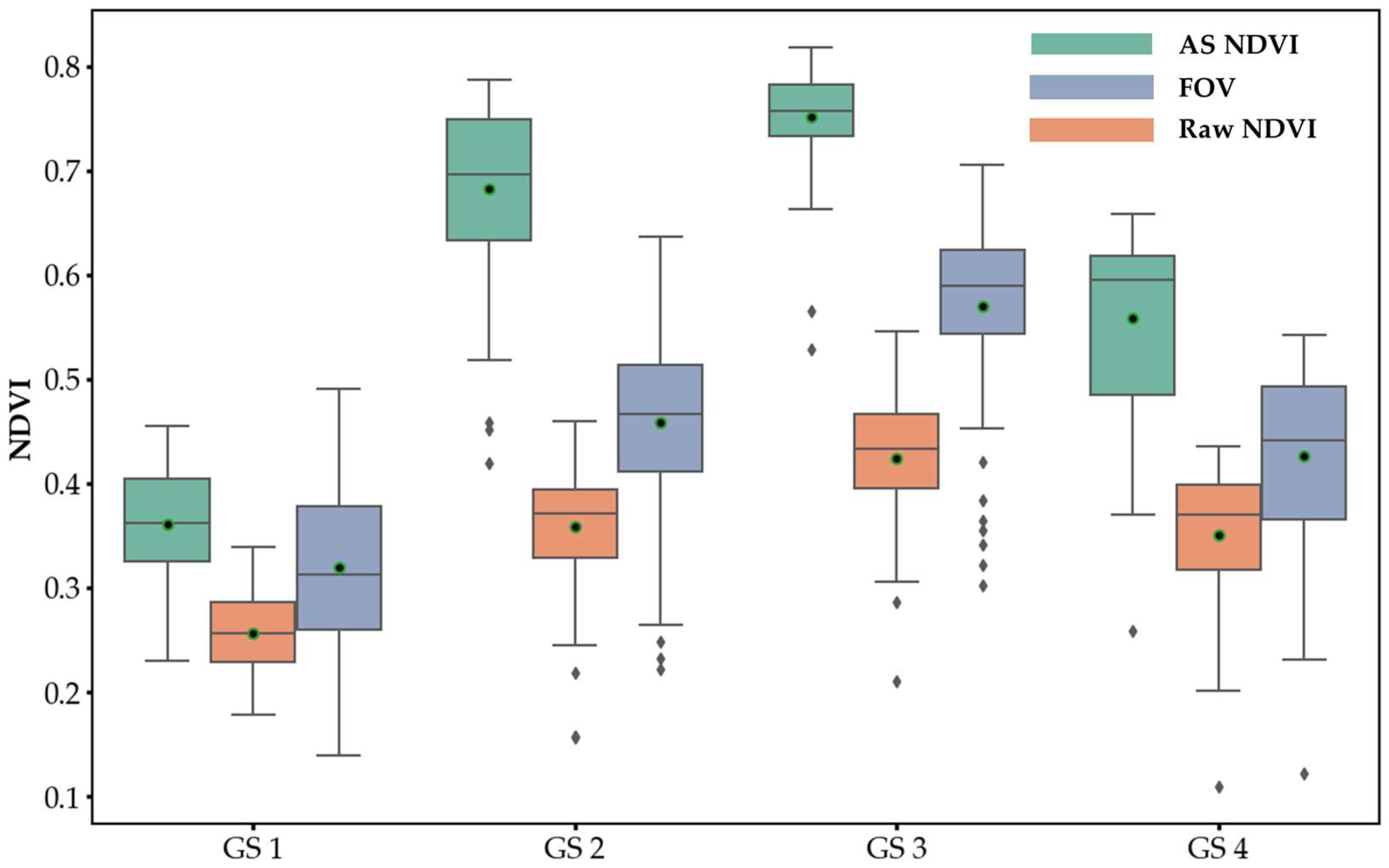
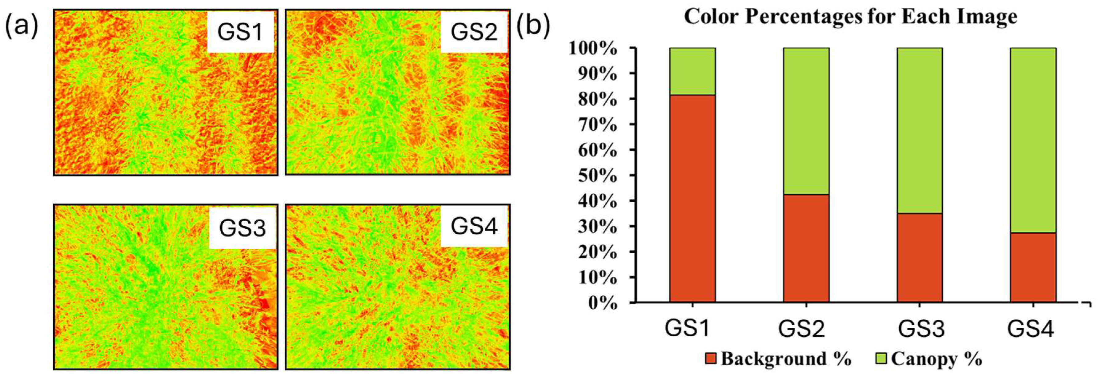
3.1. Data Characterization

Box plot and data trend graph were generated to illustrate the variations in the NDVI data as shown in Figure 9 and Figure 10, respectively, which had been processed using various enhancing techniques across the research area. These graphical representations assisted in acquiring a thorough understanding of the distribution and properties of the data. Figure 9 visualizes the distribution of NDVI values across four growth stages (GS 1 to GS 4) for three categories of data: AS NDVI, FOV, and raw NDVI. Each boxplot represents the interquartile range (IQR), where the middle 50% of the data lies, with the whiskers extending to 1.5 times the IQR. Outliers were marked as points outside the whiskers, indicating variability in the data. AS NDVI exhibits consistently higher median values and smaller variability, indicating a more refined dataset. FOV generally has intermediate medians, while raw NDVI values are comparatively lower with more outliers, reflecting greater fluctuations in unprocessed data. Across growth stages, variability increases, especially in GS3 and GS4, suggesting a broadening range of NDVI values during these later stages. This emphasizes how different processing levels influence the overall trends and reliability of NDVI measurements. The appearance of black lines in these attractive box plots indicated the average (mean) NDVI values for each separate group under examination. Kernel density plots, outlined with a variety of colors, were added to the traditional boxplot. This helped reveal even the smallest variations related to the enhancement methods. The layered density structure of the plots provides insight into the variability of NDVI values, offering a detailed view of how each technique contributes to the enhancement process. This comprehensive representation validates the superiority of combined techniques for generating consistent and reliable NDVI datasets critical for precision agriculture applications.

Figure 10 illustrates a detailed visualization of the NDVI trends over individual data samples for the same growth stages and categories (AS NDVI, FOV, and raw NDVI). Each subplot (GS 1 to GS 4) represents the temporal behavior of NDVI measurements, where AS NDVI consistently exhibits higher values and smoother trends, reflecting its refined processing. FOV shows moderate NDVI values with notable fluctuations, while raw NDVI (green) remains the lowest and most variable across samples, reflecting raw, uncorrected data. Over time, in later growth stages (GS3 and GS4), a clear upward trend in NDVI values is observed, particularly for AS NDVI and FOV, indicating increasing vegetation health. The raw NDVI remains relatively noisy throughout, emphasizing the impact of data smoothing and correction in enhancing trend clarity. Together, these graphs highlight both the distribution and dynamic trends of NDVI values, emphasizing how processing impacts data interpretation across growth stages.

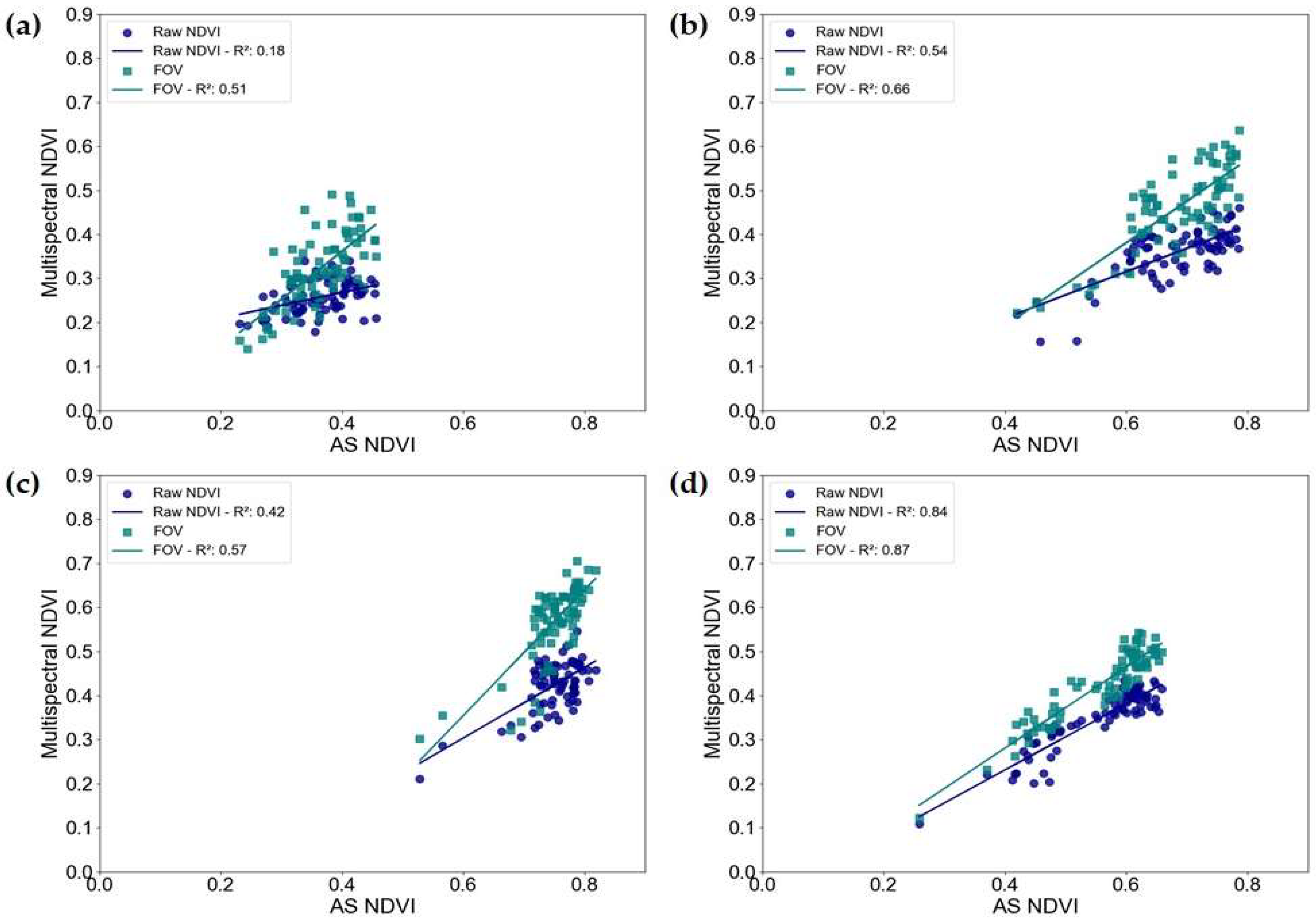
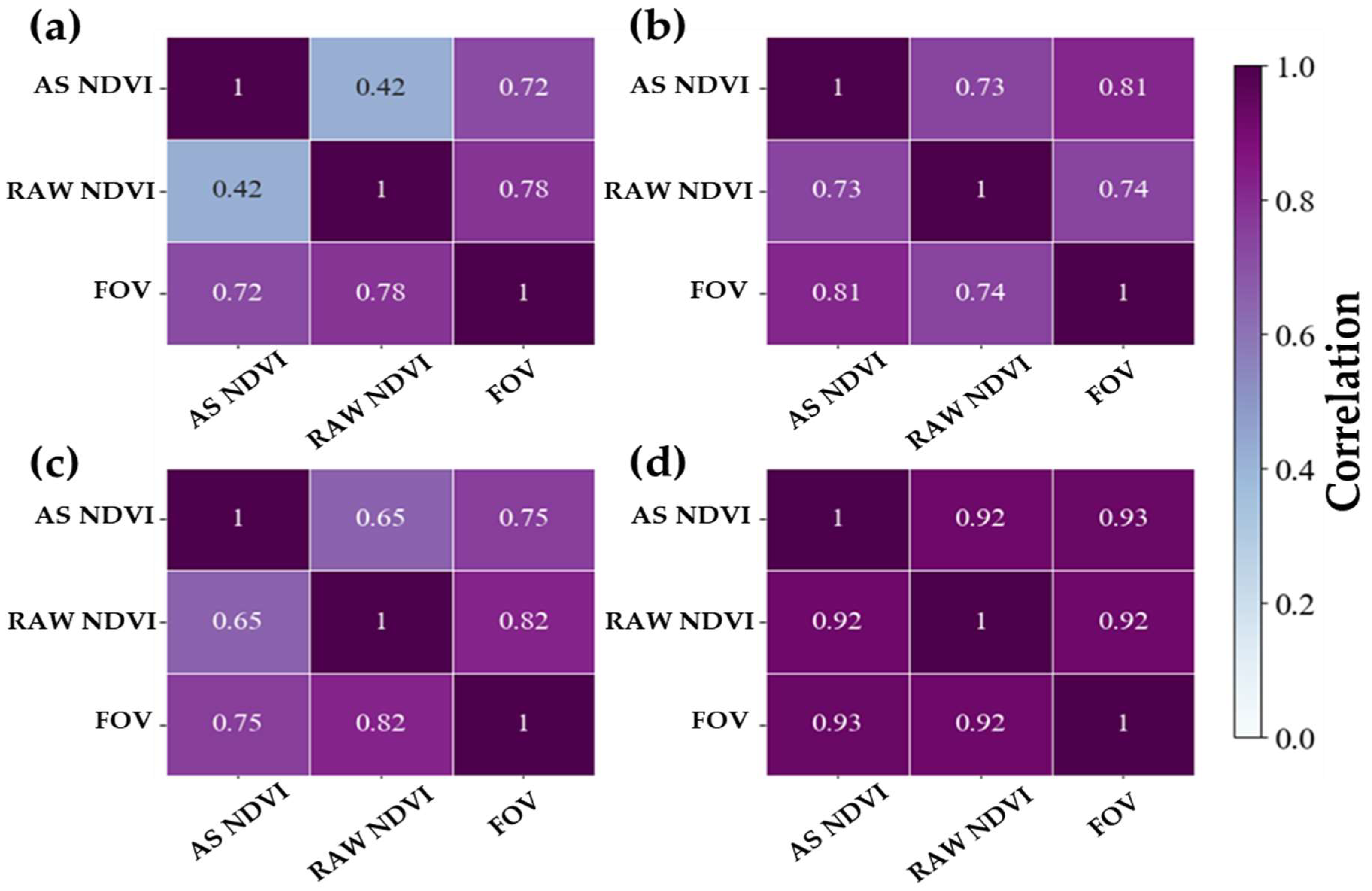
3.2. Measurement Accuracy

This study investigated the impact of various enhancement techniques on measurement accuracy across different growth stages (GS1, GS2, GS3, and GS4) based on the NDVI data collected from the active sensor (AS NDVI). The results in

Table 4. Performance metrics of NDVI enhancement techniques across four growth stages.

Growth Stages	Enhancements Techniques	Sample Number	Average NDVI	Standard Deviation (SD)	Equation	R2	RMSE
GS1	Raw data	77	0.26	0.04	y = 0.30x + 0.15	0.18	0.03
	FOV	77	0.32	0.08	y = 1.09x − 0.07	0.51	0.06
GS2	Raw data	77	0.36	0.06	y = 0.53x − 0.01	0.54	0.04
	FOV	77	0.46	0.09	y = 0.94x − 0.19	0.66	0.05
GS3	Raw data	77	0.43	0.07	y = 0.80x − 0.18	0.42	0.04
	FOV	77	0.57	0.11	y = 1.42x − 0.50	0.57	0.06
GS4	Raw data	77	0.35	0.08	y = 0.75x − 0.07	0.84	0.03
	FOV	77	0.43	0.08	y = 0.92x − 0.09	0.87	0.03

showed significant improvements in the coefficient of determination (R²) values, indicative of enhanced accuracy in the measurements. These enhancements were observed in response to the application of distinct techniques as shown in Figure 11.

For instance, in GS1, when utilizing the raw NDVI, an R² value of 0.18 was obtained. The alignment of the FOV resulted in an R² value of 0.51. In early growth stages, sensor accuracy resulted in low values due to soil background and other environmental effects. A study found that the analysis of multispectral data yielded low accuracy in maize LAI detection at early growth stages [51]. Additionally, less accuracy was found in plant vigor assessment in winter wheat at early growth stages due to the soil background effect [55]. Similarly, in GS2, the raw NDVI yielded an R² value of 0.54, while the FOV method resulted in an R² value of 0.66.

In GS3, the raw NDVI yielded an R² value of 0.42, whereas the FOV aligned NDVI resulted in an R² value of 0.57, highlighting its consistent role in enhancing measurement accuracy across different growth stages. Finally, in GS4, the raw NDVI produced an R² value of 0.84, while the FOV resulted in a 3% increase in R² value. These findings underscore the consistent effectiveness of enhancement techniques, such as applying the geometric alignment method, in optimizing measurement accuracy across various growth stages. Furthermore, Figure 12 displays canopy and background color percentages at different growth stages, highlighting the gradual decrease in background influence as plants mature. In early stages like GS1, a larger portion of the background is visible, contributing to reduced sensor accuracy, as observed in lower R² values. In early stages where there was high background visibility, the FOV alignment method had a significant effect on the NDVI calculation.

In addition, the correlation heatmap in Figure 13 provides a detailed analysis of the relationship between raw NDVI values, obtained from multispectral images before any enhancement techniques, and the values from active sensor, considered the true measurements for VIs. Comparing the enhanced NDVI values with raw NDVI values serves several critical purposes, with the primary objective being to establish a baseline assessment for evaluating the effectiveness of the FOV alignment enhancement technique, across different growth stages (GS1 to GS4). Each cell in the heatmap quantifies the linear relationship between two variables using a correlation coefficient, where values closer to 1 indicate a stronger positive correlation.

Across the growth stages, raw NDVI initially shows a lower correlation with the values of the active sensor (AS NDVI), particularly in early growth stages (GS1: 0.42). However, as the crop matures, the correlation increases (GS4: 0.92), reflecting the improved reliability of NDVI values due to enhanced canopy coverage and reduced distortions. Notably, applying FOV correction significantly improves correlations at all stages, suggesting that addressing spatial distortions is crucial for accurate NDVI measurements. By the final growth stage, enhancements have a diminishing impact, as the raw data achieves high accuracy due to the fully developed crop canopy, with the FOV method reaching a correlation of 0.93.

4. Discussion

The analysis of NDVI values across different enhancement techniques reveals significant insights into the reliability and accuracy of remote sensing data in agricultural contexts. In this study, applying FOV correction led to marked improvements in data accuracy, notably in early growth stages GS1 and GS2. Initially, raw NDVI data showed correlation coefficients averaging around 0.45 with active sensor measurements. After enhancement, this value increased substantially, reaching an average of 0.82 for FOV-corrected data. This improvement underscores how the geometric alignment method can bridge the gap between raw and ideal NDVI readings, thereby providing more reliable data for informed decision making.

Background interference from non-vegetative elements—such as soil, urban features, and other non-crop factors—significantly impacted raw NDVI readings, contributing to lower initial correlation values [50,56,57]. This interference was particularly problematic during early growth stages, as the partial canopy coverage allowed background elements to influence the spectral response. Therefore, data extraction from specified ROI is quite necessary for precision agriculture. FOV correction also proved instrumental in reducing spatial distortions commonly encountered in aerial imagery [36,58]. Aerial images often have wide FOVs, which can lead to substantial geometric distortions, particularly when capturing images from varying altitudes. This distortion was evident in raw data, with correlation values averaging only 0.48 at GS2. However, with FOV correction, this correlation rose to 0.83, aligning the data more closely with ground-truth measurements from the active sensor. These results highlight the necessity of FOV correction to achieve spatially accurate NDVI readings.

To address a deep validation of the proposed method, comparative analyses were conducted using alternative data enhancement techniques, including wavelet transformation and non-local means (NLMs). Several researchers applied these two enhancement techniques for multispectral data enhancement [59,60]. NDVI values extracted from these methods were evaluated against the NDVI data from the active sensor for accuracy. During early growth stages, raw NDVI achieved an accuracy of 18% and 54%, while wavelet transformation showed accuracies of 5% and 48%, and NML achieved 6% and 48%. These results were significantly lower than the accuracy obtained using FOV alignment, demonstrating the efficacy of the proposed method. This analysis was conducted with the dataset of early growth stages where the data have high possibilities of enhancement.

As the crops advanced to later growth stages, the reliance on enhancement techniques began to decrease. By GS4, the fully developed crop canopy naturally acted as a stabilizing factor, occluding background interference and providing consistent reflectance patterns across multiple spectral bands [50,61]. Consequently, raw NDVI values alone achieved a high correlation of 0.90 with active canopy sensor measurements at this stage. This suggests that while the enhancement method was critical for accurate early-stage NDVI measurements, mature crop canopies inherently stabilized NDVI accuracy by reducing background interference.

The FOV correction method proposed in this study has broad applications in precision agriculture, particularly in scenarios where high spatial accuracy is critical. Key application areas include the following:

• During the early growth stages, sparse canopy cover increases the influence of background soil reflectance. FOV correction minimizes this effect, enhancing NDVI accuracy and improving early stress detection [14,62].
• When integrating data from different sensors with varying FOVs, such as UAV-based sensors and ground-based multispectral devices, FOV correction ensures consistency and comparability across datasets [5,6,26,63].
• For applications requiring detailed vegetation maps, such as nutrient management and precision irrigation, FOV correction enhances spatial alignment, leading to more reliable decision-making tools [31,36,45,53].
• In controlled environments like breeding trials, where accurate assessment of plant traits is essential, FOV correction improves the precision of vegetation indices, aiding in genotype evaluation and selection [42,61,63].

These applications demonstrate the versatility and necessity of implementing FOV correction in agricultural remote sensing. The results of this study underline the importance of applying the FOV alignment method, particularly in early growth stages, to enhance NDVI reliability. Enhanced NDVI measurements in GS1 and GS2 resulted in correlation coefficients improving from 0.45 in raw data to 0.84 when the enhancement was applied. Such a significant increase in data accuracy affirms that the application of FOV correction is essential for producing consistent and reliable NDVI values, which directly supports more accurate crop health assessments. This level of data accuracy in early growth translates to better decision making for essential management practices like fertilization, irrigation, and pest control. Enhanced NDVI data allow for more precise adjustments, ultimately contributing to resource efficiency and better-targeted crop management practices. While these findings provide a strong foundation for enhancing remote sensing data, further research is essential to evaluate the applicability of these methods under diverse crop types, soil conditions, and varying environmental factors.

To further emphasize the necessity of FOV correction across different growing periods of crops, it is essential to consider the varying degrees of canopy coverage and background interference throughout the life cycle of crops [46,64]. In the initial stages, sparse vegetation and a high proportion of exposed soil make NDVI calculations highly susceptible to background noise, necessitating accurate FOV correction to enhance reflectance accuracy. As crops progress to mid-growth stages, the increasing canopy cover reduces background interference; however, variations in plant density and structural differences still contribute to inconsistencies in NDVI measurements. FOV correction during this phase ensures uniformity and comparability of vegetation indices over time. In the late growth stages, where the canopy is fully developed, the influence of soil background diminishes significantly, but sensor misalignment and potential shading effects can still impact spectral measurements. Therefore, applying FOV correction throughout all growth stages is critical for ensuring accurate, consistent, and reliable remote sensing data, ultimately improving crop health assessments and decision-making processes in precision agriculture.

While this study confirms the effectiveness of FOV correction in enhancing NDVI measurements, several limitations must be considered. The small test plot may not fully represent the variability of larger agricultural landscapes, where factors like soil heterogeneity, topography, and microclimate could impact reproducibility. Additionally, the findings are specific to the analyzed crop type, and further research is needed to assess the method’s applicability across different species with varying canopy structures. Moreover, the study focused solely on NDVI, while indices such as EVI and NDRE could provide additional insights into plant health. Evaluating FOV correction across multiple indices would enhance understanding of its broader utility. Lastly, external factors like atmospheric conditions and lighting variations may introduce uncertainties. Future research should focus on validating the effectiveness of the proposed enhancement methods across diverse agricultural landscapes and under varying climatic conditions to ensure the robustness and scalability of the approach. Additionally, further investigation into integrating multiple enhancement techniques may provide more comprehensive solutions for improving remote sensing accuracy across different growth stages.

Additionally, different time periods, geographical regions, and large-scale agricultural applications would require an assessment of the computational efficiency and scalability of the methods. This would help identify potential limitations, such as processing constrains and variability in sensor performance, and refine the techniques for broader adoption in precision agriculture. Furthermore, applying the same research methodology to different crops is expected to yield valuable insights into species-specific variations in multispectral sensor responses. Crops with denser canopies (e.g., maize, fruit orchards) may require further adjustments to sensor height and FOV alignment due to increased shadowing effects, while low-growing crops (e.g., lettuce, spinach) may experience greater background interference that could impact NDVI accuracy. Understanding how FOV alignment influences data accuracy across various crop types will be crucial for adapting this methodology to a wider range of agricultural systems.

5. Conclusions

This study highlights the important role of FOV correction in improving the accuracy and reliability of NDVI measurements in precision agriculture. This approach provided a practical solution for improving NDVI accuracy under specific conditions rather than fully resolving all FOV discrepancies. By addressing spatial distortions and background interference, particularly during early growth stages, the proposed geometric alignment method significantly enhanced the correlation between NDVI values and ground-truth active sensor measurements. Initially, raw NDVI data exhibited moderate to low correlations (~0.45) due to sensor misalignment and background effects, but after applying FOV correction, the correlation improved substantially, reaching an average of 0.82. These findings emphasize the necessity of accurate spatial alignment for extracting meaningful vegetation indices (VIs) in remote sensing applications. The study also demonstrated that early growth stages (GS1 and GS2) are particularly susceptible to background interference from soil and other non-vegetative elements, leading to lower NDVI accuracy. By GS4, as the canopy cover increased, background interference naturally diminished, and raw NDVI values alone achieved a strong correlation (0.90) with active sensor data. This suggests that enhancement techniques like FOV correction are most beneficial in early-stage NDVI assessments, while their impact diminishes as crops mature and the canopy structure stabilizes. Comparative analyses of alternative enhancement techniques, including wavelet transformation and non-local means (NLMs), further validated the superiority of FOV correction. While these methods have been widely used for multispectral data enhancement, their effectiveness in early growth stages was limited, with significantly lower accuracy compared to the FOV-aligned NDVI values. These results confirm that FOV correction provides a more reliable approach for improving NDVI measurements, particularly in conditions where background interference and sensor misalignment present challenges.

Furthermore, this study quantified and corrected spatial distortions caused by variations in sensor alignment, ensuring precise reflectance data extraction. By establishing fixed extraction coordinates and aligning passive and active sensors, the study successfully minimized inconsistencies across spectral bands. The intra-sensor geometric alignment further improved reflectance accuracy by accounting for lens displacements within the multispectral imaging system. Despite these advancements, certain limitations exist. The small test plot may not fully represent larger agricultural landscapes, where factors like soil heterogeneity, topography, and microclimate could impact reproducibility. Additionally, as the findings are specific to wheat, further research is needed to assess their applicability to other crops with varying canopy structures. Future studies should also explore the impact of FOV correction on different vegetation indices like EVI and NDRE to enhance its broader applicability.

To further validate these findings, future research should focus on testing the proposed methods across diverse geographical regions, crop types, and large-scale agricultural settings. Integrating FOV correction with advanced image processing techniques, such as machine learning-based enhancement models, could further refine NDVI calculations and improve precision agriculture applications. Additionally, evaluating the computational efficiency and scalability of these methods will be essential for their broader adoption in real-world agricultural monitoring systems. The insights gained from this research provide a strong foundation for further advancements in multispectral imaging, sensor calibration, and remote sensing applications in crop monitoring and management.

References

1. Sishodia, R.P.; Ray, R.L.; Singh, S.K. Applications of remote sensing in precision agriculture: A review. Remote Sens. 2020, 12, 3136. [Google Scholar] [CrossRef]
2. Shafi, U.; Mumtaz, R.; García-Nieto, J.; Hassan, S.A.; Zaidi, S.A.; Iqbal, N. Precision agriculture techniques and practices: From considerations to applications. Sensors 2019, 19, 3796. [Google Scholar] [CrossRef]
3. Sarkar, T.K.; Ryu, C.S.; Kang, Y.S.; Kim, S.H.; Jeon, S.R.; Jang, S.H.; Park, J.W.; Kim, S.G.; Kim, H.J. Integrating UAV remote sensing with GIS for predicting rice grain protein. J. Biosyst. Eng. 2018, 43, 148–159. [Google Scholar]
4. Montes de Oca, A.; Arreola, L.; Flores, A.; Sanchez, J.; Flores, G. Low-cost multispectral imaging system for crop monitoring. In Proceedings of the 2018 International Conference on Unmanned Aircraft Systems (ICUAS), Dallas, TX, USA, 12–15 June 2018. [Google Scholar]
5. Lu, N.; Wang, W.; Zhang, Q.; Li, D.; Yao, X.; Tian, Y.; Zhu, Y.; Cao, W.; Baret, F.; Liu, S.; et al. Estimation of nitrogen nutrition status in winter wheat from unmanned aerial vehicle-based multi-angular multispectral imagery. J. Front. Plant Sci. 2019, 10, 1601. [Google Scholar] [CrossRef] [PubMed]
6. Lu, N.; Wu, Y.; Zheng, H.; Yao, X.; Zhu, Y.; Cao, W.; Cheng, T. An assessment of multi-view spectral information from UAV-based color-infrared images for improved estimation of nitrogen nutrition status in winter wheat. Precis. Agric. 2022, 23, 1653–1674. [Google Scholar] [CrossRef]
7. Olesen, M.H.; Nikneshan, P.; Shrestha, S.; Tadayyon, A.; Deleuran, L.C.; Boelt, B.; Gislum, R. Viability prediction of Ricinus communis L. seeds using multispectral imaging. Sensors 2015, 15, 4592–4604. [Google Scholar]
8. Di Nisio, A.; Adamo, F.; Acciani, G.; Attivissimo, F. Fast detection of olive trees affected by Xylella fastidiosa from UAVs using multispectral imaging. Sensors 2020, 20, 4915. [Google Scholar] [CrossRef]
9. Yu, R.; Luo, Y.; Zhou, Q.; Zhang, X.; Wu, D.; Ren, L. Early detection of pine wilt disease using deep learning algorithms and UAV-based multispectral imagery. For. Ecol. Manag. 2021, 497, 119493. [Google Scholar] [CrossRef]
10. Radočaj, D.; Šiljeg, A.; Marinović, R.; Jurišić, M. State of major vegetation indices in precision agriculture studies indexed in Web of Science: A review. Agriculture 2023, 13, 707. [Google Scholar] [CrossRef]
11. Güven, B.; Baz, İ.; Kocaoğlu, B.; Toprak, E.; Barkana, D.E.; Özdemir, B.S. Smart farming technologies for sustainable agriculture: From food to energy. In A Sustainable Green Future; Oncel, S.S., Ed.; Springer: Cham, Switzerland, 2023. [Google Scholar] [CrossRef]
12. Nicolis, O.; Gonzalez, C. Wavelet-based fractal and multifractal analysis for detecting mineral deposits using multispectral images taken by drones. In Methods and Applications in Petroleum and Mineral Exploration and Engineering Geology; Elsevier: Amsterdam, The Netherlands, 2021; pp. 295–307. [Google Scholar]
13. Lapray, P.J.; Wang, X.; Thomas, J.B.; Gouton, P. Multispectral filter arrays: Recent advances and practical implementation. Sensors 2014, 14, 21626–21659. [Google Scholar] [CrossRef] [PubMed]
14. Haque, M.A.; Reza, M.N.; Ali, M.; Karim, M.R.; Ahmed, S.; Lee, K.; Khang, Y.H.; Chung, S. Effects of environmental conditions on vegetation indices from multispectral images: A review. Korean J. Remote Sens. 2024, 40, 319–341. [Google Scholar]
15. Park, M.J.; Ryu, C.S.; Kang, Y.S.; Jang, S.H.; Park, J.W.; Kim, T.Y.; Kang, K.S.; Ba, H.C. Estimation of moisture stress for soybean using thermal image sensor mounted on UAV. Precis. Agric. Sci. Technol. 2021, 3, 111–119. [Google Scholar]
16. Pan, Y.; Bélanger, S.; Huot, Y. Evaluation of atmospheric correction algorithms over lakes for high-resolution multispectral imagery: Implications of adjacency effect. Remote Sens. 2022, 14, 2979. [Google Scholar] [CrossRef]
17. Zhou, X.; Liu, C.; Xue, Y.; Akbar, A.; Jia, S.; Zhou, Y.; Zeng, D. Radiometric calibration of a large-array commodity CMOS multispectral camera for UAV-borne remote sensing. Int. J. Appl. Earth Obs. Geoinf. 2022, 112, 102968. [Google Scholar] [CrossRef]
18. Chen, W.; Li, X.; Wang, L. Multimodal remote sensing science and technology. In Remote Sensing Intelligent Interpretation for Mine Geological Environment; Springer: Singapore, 2022. [Google Scholar] [CrossRef]
19. Sun, W.; Ren, K.; Meng, X.; Yang, G.; Xiao, C.; Peng, J.; Huang, J. MLR-DBPFN: A multi-scale low-rank deep back projection fusion network for anti-noise hyperspectral and multispectral image fusion. IEEE Trans. Geosci. Remote Sens. 2022, 60, 1–14. [Google Scholar] [CrossRef]
20. Dian, R.; Li, S.; Sun, B.; Guo, A. Recent advances and new guidelines on hyperspectral and multispectral image fusion. Inf. Fusion 2021, 69, 40–51. [Google Scholar] [CrossRef]
21. Fu, X.; Wang, W.; Huang, Y.; Ding, X.; Paisley, J. Deep multiscale detail networks for multiband spectral image sharpening. IEEE Trans. Neural Netw. Learn. Syst. 2020, 32, 2090–2104. [Google Scholar] [CrossRef] [PubMed]
22. Coesfeld, J.; Kuester, T.; Kuechly, H.U.; Kyba, C.C. Reducing variability and removing natural light from nighttime satellite imagery: A case study using the VIIRS DNB. Sensors 2020, 20, 3287. [Google Scholar] [CrossRef] [PubMed]
23. Krus, A.; Valero, C.; Ramirez, J.; Cruz, C.; Barrientos, A.; del Cerro, J. Distortion and mosaicking of close-up multi-spectral images. In Precision Agriculture’21; Wageningen Academic Publishers: Wageningen, The Netherlands, 2021; pp. 33–46. [Google Scholar] [CrossRef]
24. Agrahari, R.K.; Kobayashi, Y.; Tanaka, T.S.T.; Panda, S.K.; Koyama, H. Smart fertilizer management: The progress of imaging technologies and possible implementation of plant biomarkers in agriculture. Soil Sci. Plant Nutr. 2021, 67, 248–258. [Google Scholar] [CrossRef]
25. Wasonga, D.O.; Yaw, A.; Kleemola, J.; Alakukku, L.; Mäkelä, P.S. Red-green-blue and multispectral imaging as potential tools for estimating growth and nutritional performance of cassava under deficit irrigation and potassium fertigation. Remote Sens. 2021, 13, 598. [Google Scholar] [CrossRef]
26. Berger, K.; Machwitz, M.; Kycko, M.; Kefauver, S.C.; Van Wittenberghe, S.; Gerhards, M.; Schlerf, M. Multi-sensor spectral synergies for crop stress detection and monitoring in the optical domain: A review. Remote Sens. Environ. 2022, 280, 113198. [Google Scholar] [CrossRef]
27. Vidican, R.; Mălinaș, A.; Ranta, O.; Moldovan, C.; Marian, O.; Ghețe, A.; Cătunescu, G.M. Using remote sensing vegetation indices for the discrimination and monitoring of agricultural crops: A critical review. Agronomy 2023, 13, 3040. [Google Scholar] [CrossRef]
28. Skendžić, S.; Zovko, M.; Lešić, V.; Živković, I.P.; Lemić, D. Detection and evaluation of environmental stress in winter wheat using remote and proximal sensing methods and vegetation indices—A review. Diversity 2023, 15, 481. [Google Scholar] [CrossRef]
29. Rojas, O. Next generation agricultural stress index system (ASIS) for agricultural drought monitoring. Remote Sens. 2021, 13, 959. [Google Scholar] [CrossRef]
30. Ahmed, N.; Zhang, B.; Deng, L.; Bozdar, B.; Li, J.; Chachar, S.; Chachar, Z.; Jahan, I.; Talpur, A.; Gishkori, M.S.; et al. Advancing horizons in vegetable cultivation: A journey from age-old practices to high-tech greenhouse cultivation—A review. Front. Plant Sci. 2024, 15, 1357153. [Google Scholar] [CrossRef] [PubMed]
31. Biney, J.K.; Saberioon, M.; Borůvka, L.; Houška, J.; Vašát, R.; Chapman Agyeman, P.; Coblinski, J.A.; Klement, A. Exploring the suitability of UAS-based multispectral images for estimating soil organic carbon: Comparison with proximal soil sensing and spaceborne imagery. Remote Sens. 2021, 13, 308. [Google Scholar] [CrossRef]
32. Roma, E.; Catania, P.; Vallone, M.; Orlando, S. Unmanned aerial vehicle and proximal sensing of vegetation indices in olive tree (Olea europaea). J. Agric. Eng. 2023, 54, 1536. [Google Scholar] [CrossRef]
33. Park, J.K.; Das, A.; Park, J.H. Application trend of unmanned aerial vehicle (UAV) image in agricultural sector: Review and proposal. Korean J. Agric. Sci. 2015, 42, 269–276. [Google Scholar] [CrossRef]
34. Tae-Chun, K.; Jong-Jin, P.; Gi-Soo, B.; Tae-dong, K. Optimal position of thermal fog nozzles for multicopter drones. Precis. Agric. Sci. Technol. 2021, 3, 122. [Google Scholar]
35. Yun, H.S.; Park, S.H.; Kim, H.J.; Lee, W.D.; Lee, K.D.; Hong, S.Y.; Jung, G.H. Use of unmanned aerial vehicle for multi-temporal monitoring of soybean vegetation fraction. J. Biosyst. Eng. 2016, 41, 126–137. [Google Scholar] [CrossRef]
36. Govender, M.; Chetty, K.; Naiken, V.; Bulcock, H. A comparison of satellite hyperspectral and multispectral remote sensing imagery for improved classification and mapping of vegetation. Water SA 2008, 34, 147–154. [Google Scholar] [CrossRef]
37. Barnes, E.M.; Sudduth, K.A.; Hummel, J.W.; Lesch, S.M.; Corwin, D.L.; Yang, C.; Daughtry, C.S.; Bausch, W.C. Remote and ground-based sensor techniques to map soil properties. Photogramm. Eng. Remote Sens. 2003, 69, 619–630. [Google Scholar] [CrossRef]
38. De Souza, R.; Buchhart, C.; Heil, K.; Plass, J.; Padilla, F.M.; Schmidhalter, U. Effect of time of day and sky conditions on different vegetation indices calculated from active and passive sensors and images taken from UAV. Remote Sens. 2021, 13, 1691. [Google Scholar] [CrossRef]
39. Cummings, C.; Miao, Y.; Paiao, G.D.; Kang, S.; Fernández, F.G. Corn nitrogen status diagnosis with an innovative multi-parameter crop circle phenom sensing system. Remote Sens. 2021, 13, 401. [Google Scholar] [CrossRef]
40. Fadadu, S.; Pandey, S.; Hegde, D.; Shi, Y.; Chou, F.C.; Djuric, N.; Vallespi-Gonzalez, C. Multi-view fusion of sensor data for improved perception and prediction in autonomous driving. In Proceedings of the IEEE/CVF Winter Conference on Applications of Computer Vision, Waikoloa, HI, USA, 3–8 January 2022; pp. 2349–2357. [Google Scholar]
41. Fang, Z.; Liang, C.; Xu, S.; Bai, Q.; Wang, Y.; Zhang, H.; Jin, B. Spatial resolution enhancement of OFDR sensing system using phase-domain-interpolation resampling method. IEEE Sens. J. 2021, 22, 3202–3210. [Google Scholar] [CrossRef]
42. Zhang, K.; Zhang, F.; Wan, W.; Yu, H.; Sun, J.; Del Ser, J.; Elyan, E.; Hussain, A. Panchromatic and multispectral image fusion for remote sensing and earth observation: Concepts, taxonomy, literature review, evaluation methodologies and challenges ahead. Inf. Fusion 2023, 93, 227–242. [Google Scholar] [CrossRef]
43. Moltó, E. Fusion of different image sources for improved monitoring of agricultural plots. Sensors 2022, 22, 6642. [Google Scholar] [CrossRef] [PubMed]
44. Guo, B.; Pi, Y.; Wang, M. Sensor correction method based on image space consistency for planar array sensors of optical satellite. IEEE Trans. Geosci. Remote Sens. 2023, 62, 5601915. [Google Scholar] [CrossRef]
45. Colaço, A.F.; Schaefer, M.; Bramley, R.G. Broadacre mapping of wheat biomass using ground-based LiDAR technology. Remote Sens. 2021, 13, 3218. [Google Scholar] [CrossRef]
46. Stamford, J.D.; Vialet-Chabrand, S.; Cameron, I.; Lawson, T. Development of an accurate low-cost NDVI imaging system for assessing plant health. Plant Methods 2023, 19, 9. [Google Scholar] [CrossRef]
47. Wei, Z.; Fang, W. UV-NDVI for real-time crop health monitoring in vertical farms. Smart Agric. Technol. 2024, 8, 100462. [Google Scholar] [CrossRef]
48. Huang, W.; Huang, J.; Wang, X.; Wang, F.; Shi, J. Comparability of red/near-infrared reflectance and NDVI based on the spectral response function between MODIS and 30 other satellite sensors using rice canopy spectra. Sensors 2013, 13, 16023–16050. [Google Scholar] [CrossRef] [PubMed]
49. Wang, R.; Cherkauer, K.; Bowling, L. Corn response to climate stress detected with satellite-based NDVI time series. Remote Sens. 2016, 8, 269. [Google Scholar] [CrossRef]
50. Prudnikova, E.; Savin, I.; Vindeker, G.; Grubina, P.; Shishkonakova, E.; Sharychev, D. Influence of soil background on spectral reflectance of winter wheat crop canopy. Remote Sens. 2019, 11, 1932. [Google Scholar] [CrossRef]
51. Liu, S.; Jin, X.; Bai, Y.; Wu, W.; Cui, N.; Cheng, M.; Liu, Y.; Meng, L.; Jia, X.; Nie, C.; et al. UAV multispectral images for accurate estimation of the maize LAI considering the effect of soil background. Int. J. Appl. Earth Obs. Geoinf. 2023, 121, 103383. [Google Scholar] [CrossRef]
52. MicaSense Incorporated. Image Processing. 2017. Available online: https://github.com/micasense/imageprocessing (accessed on 13 July 2024).
53. Hecht, R.; Herold, H.; Behnisch, M.; Jehling, M. Mapping long-term dynamics of population and dwellings based on a multi-temporal analysis of urban morphologies. ISPRS Int. J. Geo-Inf. 2018, 8, 2. [Google Scholar] [CrossRef]
54. Rouse, J.W.; Haas, R.H.; Schell, J.A.; Deering, D.W. Monitoring vegetation systems in the Great Plains with ERTS. In Third Earth Resources Technology Satellite-1 Symposium: Section A–B; Freden, S.C., Mercanti, E.P., Becker, M.A., Eds.; Technical Presentations; National Aeronautics and Space Administration: Washington, DC, USA, 1974; pp. 309–317. [Google Scholar]
55. Prey, L.; Von Bloh, M.; Schmidhalter, U. Evaluating RGB imaging and multispectral active and hyperspectral passive sensing for assessing early plant vigor in winter wheat. Sensors 2018, 18, 2931. [Google Scholar] [CrossRef] [PubMed]
56. Huang, S.; Tang, L.; Hupy, J.P.; Wang, Y.; Shao, G. A commentary review on the use of normalized difference vegetation index (NDVI) in the era of popular remote sensing. J. For. Res. 2017, 32, 1–6. [Google Scholar] [CrossRef]
57. Farias, G.D.; Bremm, C.; Bredemeier, C.; de Lima Menezes, J.; Alves, L.A.; Tiecher, T.; Martins, A.P.; Fioravanço, G.P.; da Silva, G.P.; de Faccio Carvalho, P.C. Normalized Difference Vegetation Index (NDVI) for soybean biomass and nutrient uptake estimation in response to production systems and fertilization strategies. Front. Sustain. Food Syst. 2023, 6, 959681. [Google Scholar] [CrossRef]
58. Aasen, H.; Honkavaara, E.; Lucieer, A.; Zarco-Tejada, P.J. Quantitative remote sensing at ultra-high resolution with UAV spectroscopy: A review of sensor technology, measurement procedures, and data correction workflows. Remote Sens. 2018, 10, 1091. [Google Scholar] [CrossRef]
59. Su, H.; Jung, C. Multi-spectral fusion and denoising of RGB and NIR images using multi-scale wavelet analysis. In Proceedings of the 24th International Conference on Pattern Recognition (ICPR), Beijing, China, 20–24 August 2018; pp. 1779–1784. [Google Scholar]
60. Tu, B.; Zhang, X.; Wang, J.; Zhang, G.; Ou, X. Spectral–Spatial Hyperspectral Image Classification via Non-local Means Filtering Feature Extraction. Sens Imaging 2018, 19, 11. [Google Scholar] [CrossRef]
61. Ma, Z. Sensing Technologies for High-Throughput Plant Phenotyping: A Comprehensive Review With a Case Study. Ph.D. Thesis, University of British Columbia, Vancouver, BC, Canada, 2023. [Google Scholar]
62. Wan, L.; Ryu, Y.; Dechant, B.; Hwang, Y.; Feng, H.; Kang, Y.; Jeong, S.; Lee, J.; Choi, C.; Bae, J. Correcting confounding canopy structure, biochemistry and soil background effects improves leaf area index estimates across diverse ecosystems from Sentinel-2 imagery. Remote Sens. Environ. 2024, 309, 114224. [Google Scholar] [CrossRef]
63. Xu, R.; Li, C.; Bernardes, S. Development and testing of a UAV-based multi-sensor system for plant phenotyping and precision agriculture. Remote Sens. 2021, 13, 3517. [Google Scholar] [CrossRef]
64. Sankaran, S.; Khot, L.R.; Espinoza, C.Z.; Jarolmasjed, S.; Sathuvalli, V.R.; Vandemark, G.J.; Miklas, P.N.; Carter, A.H.; Pumphrey, M.O.; Knowles, N.R.; et al. Low-altitude, high-resolution aerial imaging systems for row and field crop phenotyping: A review. Eur. J. Agron. 2015, 70, 112–123. [Google Scholar] [CrossRef]
Figure 1. Experimental wheat field for the data acquisition: (a) experiment plot, (b) nadir view of the experiment plot, and (c) different growth stages of wheat (GS1, GS2, GS3, and GS4).
Remotesensing 17 00743 g001
Figure 2. Overview of the experimental setup and data acquisition process: (a) a schematic diagram of the positions of the sensors along with data processing techniques, (b) data acquisition platform used during the early growth stage of the plants showing the height from the canopy, and (c) data acquisition during the late growth stage, highlighting the evolution of measurements and observations.
Remotesensing 17 00743 g002
Figure 3. (a) Schematic representation for the variations in projection of both sensors and consistency in the center point of FOV for both passive and active sensors in three different heights, 100, 90, and 80 cm, respectively; (b) sensor positioning; and (c) sensors mounted on the structure for the experiment.
Remotesensing 17 00743 g003
Figure 4. Overall FOV alignment process for passive and active sensors: (a) FOV projection, (b) area of interest for 90 cm height, (c) FOV in actual image, (d) plotting FOV coordinates using Python program, and (e) cropped multispectral FOV.
Remotesensing 17 00743 g004
Figure 5. Horizontal and vertical displacement based on the positions of sensors lenses.
Remotesensing 17 00743 g005
Figure 6. Comprehensive data processing flow diagram. This diagram outlines the sequential steps of data acquisition, processing, and allocation, providing a detailed overview of the entire workflow.
Remotesensing 17 00743 g006
Figure 7. Pseudo-colored image of selected regions of interest (rectangle area) for data extraction across multispectral bands (blue, green, red, NIR, and RedEdge) captured by multispectral camera in wheat field study.
Remotesensing 17 00743 g007
Figure 8. Visualization of spectral band distortion. Distortion values are relative to each band as a reference across spectral bands, during an analysis of pixel shifts towards the x and y axes across all the images.
Remotesensing 17 00743 g008
Figure 9. A box plot shows comparative visualization of AS NDVI, raw NDVI, and NDVI after FOV, showing mean NDVI values and distribution patterns across four growth stages: GS1, GS2, GS3, and GS4.
Remotesensing 17 00743 g009
Figure 10. Comparative trends of NDVI metrics (AS NDVI, FOV, and raw NDVI) across four growth stages (GS1–GS4).
Remotesensing 17 00743 g010
Figure 11. Regression analysis of NDVI enhancement techniques across four growth stages: (a) GS1, (b) GS2, (c) GS3, and (d) GS4. R2 values showing measurement accuracy for raw NDVI and FOV based on AS NDVI.
Remotesensing 17 00743 g011
Figure 12. Background visibility in multispectral images: (a) sample image from each GS for canopy and background visualization, and (b) comparison of canopy and background percentage across different growth stages (GS1 to GS4).
Remotesensing 17 00743 g012
Figure 13. Correlation coefficient heatmap between AS NDVI, raw NDVI, and FOV across growth stages: (a) GS1, (b) GS2, (c) GS3, and (d) GS4; highlighting improved measurement accuracy with FOV alignment on NDVI reliability.
Remotesensing 17 00743 g013