Combining Global Features and Local Interoperability Optimization Method for Extracting and Connecting Fine Rivers

Abstract

Due to the inherent limitations in remote sensing image quality, seasonal variations, and radiometric inconsistencies, river extraction based on remote sensing image classification often results in omissions. These challenges are particularly pronounced in the detection of narrow and complex river networks, where fine river features are frequently underrepresented, leading to fragmented and discontinuous water body extraction. To address these issues and enhance both the completeness and accuracy of fine river identification, this study proposes an advanced fine river extraction and optimization method. Firstly, a linear river feature enhancement algorithm for preliminary optimization is introduced, which combines Frangi filtering with an improved GA-OTSU segmentation technique. By thoroughly analyzing the global features of high-resolution remote sensing images, Frangi filtering is employed to enhance the river linear characteristics. Subsequently, the improved GA-OTSU thresholding algorithm is applied for feature segmentation, yielding the initial results. In the next stage, to preserve the original river topology and ensure stripe continuity, a river skeleton refinement algorithm is utilized to retain critical skeletal information about the river networks. Following this, river endpoints are identified using a connectivity domain labeling algorithm, and the bounding rectangles of potential disconnected regions are delineated. To address discontinuities, river endpoints are shifted and reconnected based on structural similarity index (SSIM) metrics, effectively bridging gaps in the river network. Finally, nonlinear water optimization combined K-means clustering segmentation, topology and spectral inspection, and small-area removal are designed to supplement some missed water bodies and remove some non-water bodies. Experimental results demonstrate that the proposed method significantly improves the regularization and completeness of river extraction, particularly in cases of fine, narrow, and discontinuous river features. The approach ensures more reliable and consistent river delineation, making the extracted results more robust and applicable for practical hydrological and environmental analyses.

1. Introduction

High-resolution remote sensing images can provide detailed and precise surface information about the Earth, which is invaluable in diverse fields such as urban planning [1], environmental monitoring [2,3], and resource management. The spatial and temporal characteristics of water bodies are subject to considerable variation due to both anthropogenic activities and natural factors, including seasonal changes, climatic fluctuations, and the occurrence of natural disasters. This is of great significance for understanding existing water resources, facilitating their rational planning and management, and supporting human livelihoods and socioeconomic activities [4,5,6]. The delineation of the extent of water bodies serves as a critical indicator of hydrological conditions within a basin, playing a pivotal role in the sustainable utilization of water resources [7,8]. Leveraging remote sensing technologies enables the timely detection of spatial and temporal distribution patterns of water bodies, which is essential for informed decision-making in water resource management. Moreover, the extraction of key hydrological parameters—such as the shape, location, and surface area of water bodies—not only aids in the conservation and efficient use of water resources but also contributes to the assessment and mitigation of natural hazards, including floods. Additionally, such information is instrumental in guiding agricultural practices within watersheds and surrounding regions [8,9,10,11,12,13]. However, due to the similarity between the spectral characteristics of water bodies and the surrounding features, as well as the complexity of the surface conditions and other images, there are unavoidable river breaks and incomplete phenomena in the results of the existing water body extraction methods [14,15,16,17]. Thus, it is of great research value to further explore the river complete succession method to realize the comprehensive and accurate extraction of water body information [18,19].

With the rapid advancement of remote sensing technology, the automatic extraction of water bodies from remote sensing imagery has emerged as a prominent research focus, garnering significant attention from scholars worldwide. In response to the challenges associated with accurate water body delineation, numerous methodologies have been proposed to enhance the precision and efficiency of water body extraction [20]. These methods are categorized into three main groups: spectral feature-based methods, machine learning classification methods, and deep learning-based methods [21,22]. (1) Spectral feature-based and classification methods extract water bodies by selecting appropriate spectral bands and constructing models derived from the spectral reflectance characteristics of water, including the single-band threshold method, multi-band water index method, and multi-band inter-spectral relationship method. The single-band threshold method classifies water by setting a threshold on a specific band, but its accuracy is sensitive to threshold selection and may suffer from misclassification due to shadows, clouds, or ripples [23]. Multi-band water index methods, such as NDWI and MNDWI, use combinations of spectral bands to calculate indices that differentiate water from other features [23,24]. However, the effectiveness of these methods depends on appropriate band selection, as spectral interactions between features can lead to errors. The multi-band inter-spectral relationship method improves accuracy by analyzing spectral differences and spatial distributions, combining both spectral and spatial information. Nonetheless, these methods rely heavily on spectral distinctions, and similar spectral features between water and surrounding elements can cause confusion, particularly when extracting fine-scale water bodies. (2) The machine learning classification method is mainly used to extract water body features, combined with support vector machine (SVM), decision trees [25,26], and object-oriented classification [27] to realize automatic water extraction [28]. The performance of SVM decreases when features are insufficiently or inaccurately extracted. Decision trees classify water bodies based on spectral, texture, and shape features but are sensitive to the number of nodes and feature selection [29]. While increasing the number of nodes can improve accuracy, excessive nodes may lead to overfitting and unstable results, especially under varying environmental conditions. Object-oriented methods treat homogeneous pixels as objects, preserving spatial structure and improving the accuracy of river shape and boundary extraction compared to pixel-level methods. However, their performance depends on parameters like segmentation thresholds and object size, requiring expert tuning or repeated trials. Additionally, these methods are sensitive to image quality and resolution, increasing computational costs. (3) Deep learning-based methods use deep neural networks to automatically learn multilevel feature representations in images with strong characterization and generalization capabilities and are suitable for complex scenes and large-scale data processing [30]. Convolutional neural networks (CNN), U-Net, and fully convolutional networks (FCN) have been widely applied for water extraction across various scenarios [31]. Advanced models like the self-attention capsule feature pyramid network (SA-CapsFPN) multi-scale feature fusion strategy have demonstrated superior performance in extracting water bodies of different shapes and sizes. However, these approaches require large datasets and significant computational resources, particularly for high-resolution remote sensing images. Additionally, the numerous hyperparameters involved demand extensive experimentation for optimization, increasing time and resource costs.

Since water results can be extracted from remote sensing images, they do not completely match with the real data. Some rivers are missed and some ponds are misrecognized as paddy fields. Therefore, water optimization methods have been explored further improving the precision of water results, including the use of feature optimization, model optimization, and data fusion methods. The feature selection optimization method improves the recognition accuracy of water bodies by carefully selecting the most representative and distinguishable features [32,33]. This method integrates the spectral, textural, morphological, and spatial features of water bodies to ensure the comprehensiveness and accuracy of water body information. Ref. [34] explored the augmented normalized difference water index (ANDWI), which leverages RGB, NIR, and SWIR1-2 bands alongside the dynamic Otsu threshold to enhance water and non-water pixel differentiation. The model improvement method aims to optimize the network structure and adjust the training strategy by screening and combining the most representative features, adjusting the learning rate, the number of iterations, and other parameters, so that the model focuses more on the key information, which can better adapt the model to the distribution of the data and improve the generalization ability of the model. Ref. [35] proposes EDWNet, an encoder–decoder semantic segmentation network for high-precision water body extraction, integrating cross-layer feature fusion (CFF) for improved edge segmentation, the global attention mechanism (GAM) to minimize information diffusion, and a deep attention module (DAM) to enhance global perception and refine water body features. The data fusion optimization method [36] provides more comprehensive and rich information by integrating data from multiple sources. Through data fusion, the advantages of various types of data can be fully utilized to make up for the deficiencies of a single data source, thus obtaining more accurate and complete information about the water body. Ref. [37] enhanced the reliability of water body extraction from C-band SAR images by integrating polarized VV/VH data with DTM, DSM, and land use information to limit backscatter sensitivity.

In summary, significant advancements have been made in the optimization techniques for water body extraction from high-resolution remote sensing images. However, several challenges and limitations remain to be addressed. First, in complex environments, existing water extraction methods are highly susceptible to natural factors such as seasonal variations, radiometric inconsistencies, and shadow occlusions. These factors often lead to spectral confusion between water bodies and surrounding features, resulting in misclassification of non-water objects with similar spectral characteristics. Once such errors occur during the initial extraction, subsequent optimization techniques may struggle to rectify these inaccuracies. Second, current optimization methods for high-resolution remote sensing images still exhibit limitations, such as the omission of small water bodies and the presence of gaps in larger water areas post-optimization. These issues contribute to incomplete extraction results, thereby compromising the overall accuracy of water body delineation. Third, the diverse characteristics of water body environments further complicate optimization efforts. Variations in morphology, size, depth, and other physical properties make it challenging for global optimization techniques to achieve consistent performance across different water body types. This is particularly problematic for fine-scale water bodies which, due to the spatial resolution limitations of remote sensing imagery, often appear as narrow, linear features. Such characteristics increase the likelihood of river discontinuities during the extraction process, where sections of rivers are not continuously represented, ultimately affecting the comprehensiveness and reliability of the optimization outcomes.

To solve the above problems, this paper focuses on preliminary optimization based on Frangi filtering and the GA-OTSU algorithm as well as the depth optimization of disconnection and connection for local interconnection. It focuses on the extraction and optimization of water bodies from high-resolution remote sensing images, proposing a preliminary optimization method combining Frangi filtering and the GA-OTSU threshold segmentation algorithm, and a depth optimization method using connectivity domain labeling and SSIM structural similarity metrics, addressing challenges such as spectral confusion and optimization.

The main contributions of this paper are as follows:

(1)

This paper proposes a preliminary optimization method for linear water bodies combining the Frangi filtering algorithm and an enhanced GA-OTSU threshold segmentation algorithm. Firstly, the Frangi filter is employed to amplify the linear feature responses of rivers. Subsequently, a genetic algorithm (GA) is incorporated into the traditional OTSU thresholding framework to accelerate the optimization process and achieve a more stable, non-linear determination of the optimal segmentation threshold. This approach effectively separates the target water bodies from the background, enabling more comprehensive extraction of riverine linear features.

(2)

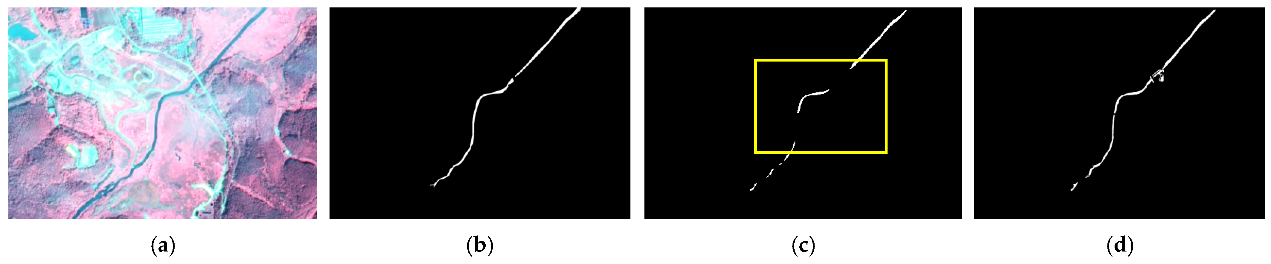
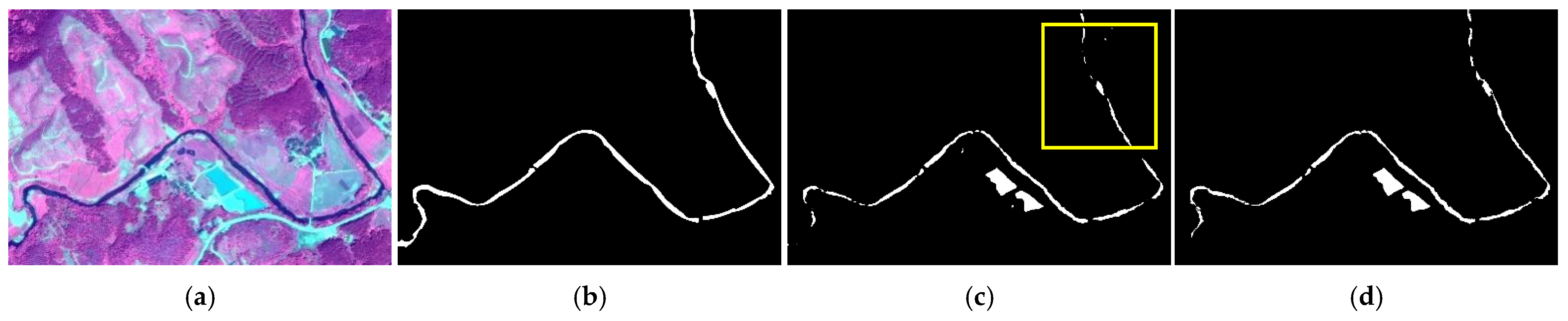
A depth optimization method for fine rivers has been designed, using the connectivity domain labeling algorithm combined with SSIM structural similarity metrics. First, the river endpoints are identified from the linear feature map, and potential disconnected regions are detected. To assess structural similarity between endpoints, structural similarity index (SSIM) values are computed for the outer rectangular sub-images of these regions. Endpoints exhibiting high structural similarity are subsequently connected, effectively restoring discontinuous river segments and achieving refined optimization of fine-scale river networks.

2. Related Studies

2.1. Water Extraction

Spectral feature-based methods mainly include the single-band threshold method [38,39], multi-band water index method [40,41], and multi-band inter-spectral relationship method [42,43]. The single-band threshold method classifies the image into water and non-water bodies by setting a threshold value to achieve water classification. The key to this method is the determination of the optimal threshold, which determines the accuracy and precision of the results. Classification is based only on a single band, which may lead to misclassification due to changes in the gray level caused by shadow, clouds, ripples, etc. Multi-band water index methods utilize reflectance of different bands in multispectral remote sensing images to distinguish water from other features by calculating specific water indices (e.g., NDWI, MNDWI, etc.) [23,24]. These methods require the selection of a suitable combination of bands to construct the index. However, the selection of different bands may have an impact on the accuracy of water extraction, since features are prone to interact with each other, leading to misclassification [44]. The multi-band inter-spectral relationship method extracts waters by analyzing the spectral differences and spatial distribution between pixels and comprehensively utilizes spectral and spatial information to improve the accuracy and reliability of river extraction [45]. These methods have a high dependence on the spectral features of the water body and the surrounding features may have similar spectral features to the water body in some bands, which leads to confusion in the extraction process and affects the accuracy of the extraction results; in addition, it is not suitable for the extraction of fine water bodies at small scales.

The performance of water extraction based on machine learning classification methods varies with different classifiers [46,47,48]. Paul et al. [49] used SVM (support vector machine), K-means clustering, and RF (random forest) methods to extract water information, showing that SVM achieved superior results. These methods require a large number of training samples, which may consume a lot of manual resources. When the features are not sufficiently or accurately extracted, the performance of the SVM classification model decreased. A decision tree is a classification method that uses a tree structure to classify water characteristics and then identify water [30]. For river extraction, the decision tree can automatically determine which regions may belong to rivers based on the spectral, texture, shape, and other water features in the remote-sensing image [50]. When using a decision tree for image classification, the number of nodes and the feature values have a great influence on the classification accuracy. When the node number is increased, the accuracy tends to be stable. However, too many nodes will cause low classification results [51,52]. As it is subject to problems of overfitting, insensitivity to the input data, and the involvement of multiple feature types and environmental conditions, the decision tree algorithm may not capture all the complex relationships, resulting in unstable results. Object-oriented methods [53] consider homogeneous pixels in remote sensing images as objects and realize effective water extraction by segmenting and classification. Compared with the traditional pixel-level classification methods, object-oriented methods can better retain the spatial structure and morphological information of features, which is conducive to accurately extracting their shapes and boundaries. However, the performance of such methods is affected by many parameters, such as segmentation threshold, object shape and size, etc. Choosing the appropriate parameters usually requires experience or repeated trials, which increases the time cost and, the method is sensitive to the quality and resolution of the input image [54].

Deep learning has been introduced to generate water extraction models based on the CNN [55], U-Net, FCN [56], etc. These methods can be used to extract various types of water in multiple scenarios. Yu [57] proposed a novel self-attention capsule feature pyramid network (SA-CapsFPN). The experimental results show that this network outperforms existing methods such as FCN, U-Net, and DeepLab [58] in extracting water with different shapes, areas, and sizes. However, these methods require a large amount of sample data and computational resources to train and optimize the network model, especially for high-resolution remote-sensing images. Moreover, the models usually contain many hyper-parameters, and adjusting the hyper-parameters to obtain the best performance requires a large amount of experimental and time costs. Further, the model generalization ability needs to be enhanced.

2.2. Water Optimization

The feature selection optimization method integrates the spectral, textural, morphological, and spatial features of water bodies to ensure the comprehensiveness and accuracy of water body information. By integrating these features, Wu et al. [59] introduced the morphological white top hat transform operation based on MNDWI and constructed the morphological narrow water index (MLWI), which is capable of recognizing narrow waters in MNDWI images from shadows. This method is affected by surrounding disturbing features, and the model accuracy and generalization ability need to be improved.

The model improvement and optimization method aims to optimize the network structure and adjust the training strategy by screening and combining the most representative features, adjusting the learning rate, the number of iterations, and other parameters, so that the model focuses more on the key information, which can make the model better adapted to the distribution of the data, and improve the generalization ability of the model. This type of method pays less attention to the edges, since vegetation or shadow may easily to be misdeteced as water.

The data fusion optimization method [36] provides more comprehensive and rich information by integrating data from multiple sources. Through data fusion, the advantages of various data sources can be fully utilized to make up for the deficiencies of a single source, thus obtaining more accurate and complete information about the water body. The process of data fusion involves several steps, including data preprocessing, data alignment, feature extraction, and fusion algorithm selection. Through the data fusion optimization method, complementary multi-source data can be fully utilized to improve the accuracy and reliability of water body extraction [60]. At the same time, this method also helps to better understand and analyze the distribution and changes of water bodies, providing a more scientific basis for the rational use and protection of water resources. Li et al. [23] proposed a novel accurate water body extraction method based on unsupervised deep learning and multi spectral imagery by analyzing the data from GF-2 and Sentinel-2 with an optimized joint teaching (ACT) deep learning method; this utilizes peer-to-peer networks with different learning abilities during the training process to effectively filter errors introduced by noisy labels.

3. Methodology

3.1. Overall Framework

The water body optimization method used in this paper is shown in Figure 1. Firstly, the water body is extracted from the high-resolution remote sensing image by the classification method to obtain the initial extraction result of the water body. The linear features and linear tributaries in the original image are obtained by Frangi filtering and the GA-OTSU method. Then, the skeleton of the river is extracted, and the possible broken flow area is obtained according to the river endpoint. To address these discontinuities, the structural similarity index (SSIM) and a connected domain labeling algorithm are employed to reconnect and supplement broken river segments, yielding refined optimization results. Then, the water body is classified by a clustering method, and topological inspection and spectral inspection of water bodies and fine optimization results are carried out, and the small area of noise interference is eliminated to improve the accuracy of water body optimization.

3.2. Preliminary Optimization

A preliminary optimization method for linear water bodies combining the Frangi filtering algorithm and an improved GA-OTSU threshold segmentation algorithm is proposed. It will be applied to initial water extraction results. Firstly, water bodies are extracted from high-resolution remote sensing images using the deep learning classification method and the initial extraction results of water bodies were obtained automatically. In comparison to many networks, U-Net is stable for water classification. Therefore, the initial water body is extracted by U-Net. To enhance the linear features of the river, the Frangi filter is applied, followed by the extraction of linear structures from the image using the Hessian matrix and eigenvalue decomposition. This approach enables the identification of river-like features by emphasizing their inherent linearity and geometric characteristics. Initially, a Gaussian filter is applied to denoise the image, followed by Frangi filtering to enhance linear structures such as rivers. Subsequently, the GA-OTSU threshold segmentation algorithm is employed to effectively distinguish target water bodies from the background, generating a preliminary linear feature map of rivers. This feature map is then cross-validated with spectral characteristics by integrating remote sensing imagery with the initial extraction results. Finally, the average RGB values of water pixels are utilized to refine the identification of linear river tributaries, producing the preliminary optimization results.

3.2.1. Frangi Filtering to Extract Linear Features

The Frangi filtering algorithm can enhance the water body features, highlight the water body boundary and detail information, making the water more clearly visible in the image. In this paper, Frangi filtering is used as a river extraction method to highlight the water body features of linear rivers.

First, the image is Gaussian filtered to filter and reduce the noise in a local region of the image. Then, the Hessian matrix of each pixel in the image is calculated. This matrix describes the second-order derivative local information of the image and calculates its eigenvalues ${\lambda }_1$ and ${\lambda }_2$ that can describe the fine line structure well, including the inverse and intensity of the local structure of the image.

Frangi filtering detects fine linear structures in an image by comparing the eigenvalues ${\lambda }_1$ and ${\lambda }_2$. Generally, if the difference between the eigenvalues is large, it indicates that there is a fine linear structure at the pixel. The response function shown in Equation (1) is calculated based on the eigenvalues to indicate the presence and intensity of the fine linear structure in the image.

$$S=\sqrt{R_b^2-{\lambda }_2^2}$$

(1)

where $R_b=$ is defined as the ratio of the eigenvalues $R_b={\lambda }_1/{\lambda }_2$.

The response function is constructed using S, ${\lambda }_1$ and ${\lambda }_2$. By adjusting the response function, the background points and isolated noise points can be suppressed. As a result, redundant information can be removed that may interfere with the analysis, without interfering with the main target area. At the same time, Frangi filtering has a strong response ability to the target area that needs to be enhanced.

3.2.2. GA-OTSU to Optimize Thresholds

To further improve the accuracy of water body extraction in linear features, a GA-OTSU segmentation algorithm is designed. The GA-OTSU threshold segmentation algorithm enhances the speed of the OTSU method by using a genetic algorithm (GA) to nonlinearly and stably find the best segmentation threshold t, thus enabling more complete extraction of the target of interest and better separation from the background features. The specific steps of the algorithm are described as follows:

• Digital Coding: The image is coding with pixel gray values ranging from 0 to 255, and 8-bit binary representation.
• Determination of Population Size: The population size represents the total number of individuals in each generation. Typically, it is set to 8, with each category randomly initialized to generate 8 different chromosomes.
• Category Decoding: Decoding each category is the reverse process of the encoding operation. In the GA-OTSU algorithm, the inter-class variance between the target and background in the remote sensing image is used as the key index to evaluate category fitness by the inter-class variance formula, and selection and cumulative probabilities are determined accordingly. Additionally, 8 random numbers are generated for subsequent processing. The larger the variance of the category, the higher its fitness, making it more likely to participate in subsequent genetic operations. This step provides a critical basis for the algorithm to identify the optimal segmentation threshold.
• Genetic Operations: Crossover, selection, and mutation are operated to generate offspring that are closer to the optimal solution. The crossover rate, a key factor in the exchange of information between chromosomes, must be set appropriately. Based on experimental verification, a crossover rate of 80% is typically effective. The mutation operation, which occurs randomly, selects a point on the chromosome and alters it to compensate for any potential information loss during the selection and crossover steps. This ensures the global search ability of the algorithm and helps to effectively obtain the optimal segmentation threshold t.

GA-OTSU makes full use of the global search ability and optimization properties of the genetic algorithm. By setting a suitable fitness function and genetic operation, the algorithm can search for the optimal segmentation thresholds quickly and stably. In this process, the algorithm not only takes into account the statistical distribution of the pixel values but also incorporates the spatial information and structural features of the image, so that it can more accurately identify the boundaries between the linear water body and the other features. By using the GA-OTSU algorithm, the features of linear water bodies such as rivers can be effectively extracted to obtain a clear map of linear features of fine rivers.

3.3. Depth Optimization for Succession of Broken Rivers

The preliminary results enhance river delineation and improve the representation of fine-scale rivers. However, due to the complexity of the surrounding environment, rivers may be obscured by vegetation, building shadows, or other occlusions, leading to interruptions in the extracted river network and discontinuities in watershed representation. Consequently, the current extraction results do not fully meet the requirements of practical applications.

To address these challenges, this paper proposes a local interoperability-based broken stream succession algorithm for further optimization, aimed at enhancing the integrity and continuity of river extraction. Building upon the preliminary water extraction results, the algorithm facilitates the succession of disconnected river segments. First, river breakpoints and potential discontinuities are identified through skeleton refinement. Then, leveraging the connected domain labeling algorithm based on depth-first search (DFS) and the structural similarity index (SSIM), the algorithm reconnects discontinuous river sections, yielding more complete and continuous water body extraction.

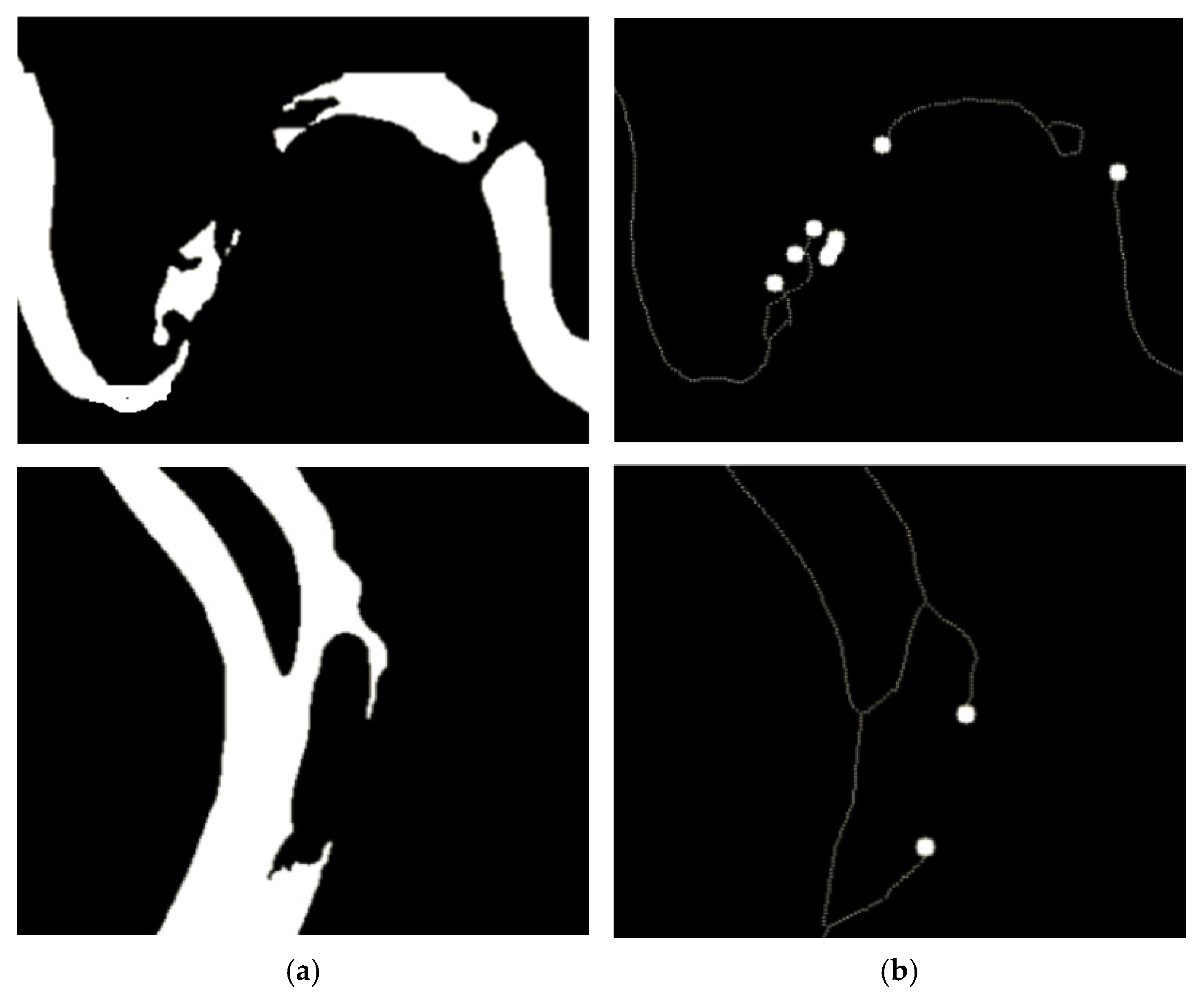
3.3.1. River Skeleton Refinement Extraction

This paper employs the Zhang–Suen fast parallel thinning algorithm to extract skeleton information from the image. The core principle of the Zhang–Suen thinning algorithm is to iteratively identify and select the skeleton center points by examining the correlation between each pixel and its eight adjacent neighbors. To extract the image skeleton, all contour pixels are processed using the parallel thinning algorithm, which operates through iterative local operations. By performing two sub-steps iteratively, the image is gradually thinned until no further thinning is possible, thereby extracting the skeleton information from the image.

In the first step, if the contour pixels meet the following conditions as shown in Equation (2), these contours will be deleted. The conditions are as follows:

$$\begin{array}{l}{S}_1:2\le N(P_1)\le 6\\ S_2:M(P_1)=1\\ S_3:P_2\times P_4\times P_6=0\\ S_4:P_4\times P_6\times P_8=0\end{array}$$

(2)

where $N(P_1)$ represents the number of non-zero neighbors of $P_1$, $M(P_1)$ is the number of times when the values of these points change from 0 to 1 if the points are ordered from $P_2~P_9$.

In the second step, only S₃ and S₄ in the first step need to change into Equation (3), and the others remain unchanged.

$$\begin{array}{l}{S}_3:P_2\times P_4\times P_8=0\\ S_4:P_2\times P_6\times P_8=0\end{array}$$

(3)

Then, the above two steps comprise a complete iteration. The iterative process will continue until there are no points that need to be removed. At this time, the area composed of the remaining pixels is the refined skeleton.

The preliminary result image is cut layer by layer by the Zhang–Suen fast parallel thinning algorithm. Based on maintaining the overall shape of the image, some redundant pixels are removed at the same time. Therefore, the image is gradually simplified. Finally, a clear skeleton of the river line is presented, that is the center line of the river. The algorithm reveals the main structure and shape information of the river. The skeleton obtained by thinning technology helps to highlight the main feature points of the river. As shown in Figure 2, the endpoints, intersections, and inflection points of the river are interrupted in the skeleton image. The interference of redundant information on image analysis and feature extraction is avoided.

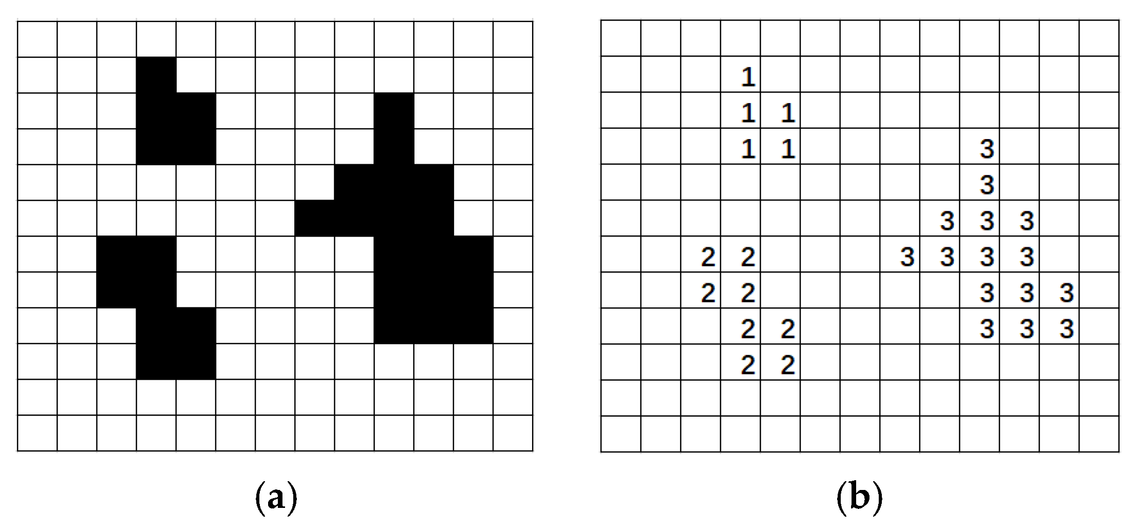
3.3.2. Connected Domain Labeling Based on Depth-First Search (DFS)

In this paper, a connected domain labeling algorithm based on depth-first search is adopted to ensure the break points are connected correctly. By traversing each pixel and based on the adjacency relationship, the connected pixels with the same value are grouped into the same connected region. Then, a unique label is assigned to each region. In the connected domain labeling algorithm, the depth-first search can effectively mark and distinguish the connected domains in the image.

The basic steps of the connected domain labeling algorithm based on depth-first search (DFS) include initialization, scanning, searching, updating, and iteration. First, an empty tag list is created and initialized to store the labels of different connected regions. Then, by scanning the image, each unvisited pixel is traversed to perform the depth-first search. The depth-first search begins by selecting an unvisited pixel as the starting point and assigning it a new connected region marker. The pixel is marked as accessed. Recursively, all adjacent unvisited pixels are accessed and marked with the same connected region marker. This process continues until there are no more unvisited adjacent pixels. Once the depth-first search for a connected region is completed, the tag list is updated by adding a new connected region label. The above process is repeated until all remaining pixels in the image are accessed and marked. At the end of this procedure, each connected region is assigned a unique label.

As shown in Figure 3 the homogeneous region is marked in the four connected region in this paper. First, a pixel that needs to be marked is selected as the seed point, and the DFS algorithm is applied to propagate outward from this point, identifying all the connected pixels within the region. These connected pixels are then marked as part of the same connected domain. Next, a pixel from another unmarked connected domain is selected as a new seed point. This process is repeated until all regions have been traversed, ensuring that all connected domains are labeled.

3.3.3. Structural Similarity (SSIM) Algorithm

Finally, the structural similarity (SSIM) [61] index is used in this paper to evaluate image quality. Based on the three indices of average brightness, contrast, and structure, the structural similarity of pixel values in each two regions is measured. The value range of SSIM is [0, 1]. The closer the value is to 1, the higher the regions similarity. Therefore, the SSIM index is used to evaluate similarity of the connected domains and connect similar regions to improve the continuity of the disconnected rivers.

The structural similarity index (SSIM) is a full-reference (FR) image quality assessment model designed to evaluate the similarity between two luminance images I₁(i, j) and I₂(i, j). The image size, M × N, $Q(i,j)$, is a multiplicative combination of three terms—luminance similarity l(i, j), contrast similarity c(i, j), and structure similarity s(i, j). SSIM can be calculated using Equation (5).

$$Q(i,j)=l(i,j)\cdot c(i,j)\cdot s(i,j)$$

(4)

$$SSIM(I_1,I_2)={\displaystyle \frac{1}{MN}}{\displaystyle \sum _{\mathrm{i}=1}^M{\displaystyle \sum _{\mathrm{j}=1}^{N}Q\left(i,j\right)}}$$

(5)

Based on the river endpoints, the circumscribed rectangle surrounding the potential river break regions and the corresponding image subgraph can be determined. A pair of river endpoints is considered as a group, and these endpoints are extended outward by a preset distance. This allows for the calculation of the two oblique diagonals of the circumscribed rectangle, which are used to assess the position and size of the rectangle and the corresponding image subgraph. For each sub-image, the SSIM (structural similarity index) value of each pixel is computed. By setting a predefined threshold, the SSIM value of a pixel is compared to the SSIM value range of the two endpoints. If the pixel’s SSIM value falls within this threshold range, it is considered similar in structure to the two endpoints and is categorized as part of the same water area. Using this approach, pixels that exhibit similar structural characteristics to the two endpoints are identified. These identified pixels are then marked using the connected domain algorithm to extract distinct connected regions within the subgraph. If both endpoints are assigned the same label, they are considered part of the same connected domain, and the corresponding connected region is incorporated into the preliminary optimization results. The final depth optimization results for the water body are then derived.

3.4. Nonlinear Water Optimization Based on K-Means Clustering and Spectral–Morphological Joint Inspection

The purpose of nonlinear water optimization is to supplement some missed water bodies and remove some non-water bodies. This optimization process covers K-means clustering segmentation, topology and spectral inspection, and small-area removal.

First, K-means clustering segmentation is executed through the image to segment the image finely. The K-means clustering algorithm is used to calculate the Euclidean distance between similar pixels and divide the pixels in the image into different categories. For general water body extraction, K = 4. For more complex environments, such as urban regions with mixed land cover, K = 5 or 6 may improve separation between water and shadowed areas [62]. Due to the significant difference between the spectrum of the river in the image and the background, the river can be quickly extracted from the original image by K-means clustering segmentation.

To further refine the extracted water bodies, an optimization process integrating topological and spectral inspection is implemented. First, topological verification is performed by comparing the water body classification results obtained through K-means clustering with those derived from the deep optimization process. The analysis identifies intersecting and non-intersecting regions between the two datasets. Intersecting regions are directly classified as water bodies, while non-intersecting regions undergo spectral verification and correction to ensure accurate classification. The verified non-intersecting water bodies are then incorporated into the final optimized extraction results.

Additionally, a small area removal process is applied to eliminate noise-induced artifacts. Since natural water bodies such as rivers and lakes typically occupy relatively large areas, small water patches are often artifacts caused by factors such as data noise, image resolution, or misclassification. To mitigate these issues and enhance the accuracy of water body extraction, a size-based threshold is defined relative to the image scale, ensuring that water regions smaller than the threshold are removed. This step not only minimizes classification errors and enhances extraction accuracy but also eliminates unintended or insignificant water segments, leading to a more precise, well-defined, and practically relevant final extraction. Consequently, the proposed method significantly improves the reliability and accuracy of water body delineation in high-resolution remote sensing imagery.

4. Experiment Analysis

4.1. Dataset

The Gaofen Image Dataset (GID) [63] is a large-scale high-resolution remote sensing image land cover dataset based on GF-2 satellite data. The GID dataset consists of 150 GF-2 satellite images from over 60 different cities across China, covering various regions and time periods, that provides high representativeness and diversity. With spatial resolutions ranging from 1 m to 10 m, the dataset can capture fine details of urban land cover. It is widely used in Gaofen image analysis and machine learning research. The GID dataset includes various types of Gaofen images, such as satellite, aerial, and ground-based photographs, encompassing a wide range of geographical environments and scenes, including urban areas, farmland, water bodies, and forests.

4.2. Evaluation Indicators

In order to quantitatively evaluate the accuracy of the optimization results, this paper selects the overall accuracy OA, integrity CM, accuracy CR, and comprehensive value F1 as the evaluation indicators. The evaluation indicators are defined as follows:

$$OA={\displaystyle \frac{P_T+N_T}{P_T+N_T+P_F+N_F}}$$

(6)

$$CR={\displaystyle \frac{P_T}{P_T+P_F}}$$

(7)

$$CM={\displaystyle \frac{P_T}{P_T+N_F}}$$

(8)

$$F_1={\displaystyle \frac{2\times E_{CR}\times E_{CM}}{E_{CR}+E_{CM}}}$$

(9)

where, $P_T$ represents the number of water pixels correctly classified, $P_F$ represents the number of pixels that are not water but classified as water, $N_F$ represents the number of pixels that should be water but classified as background, $N_T$ represents the number of background pixels correctly classified.

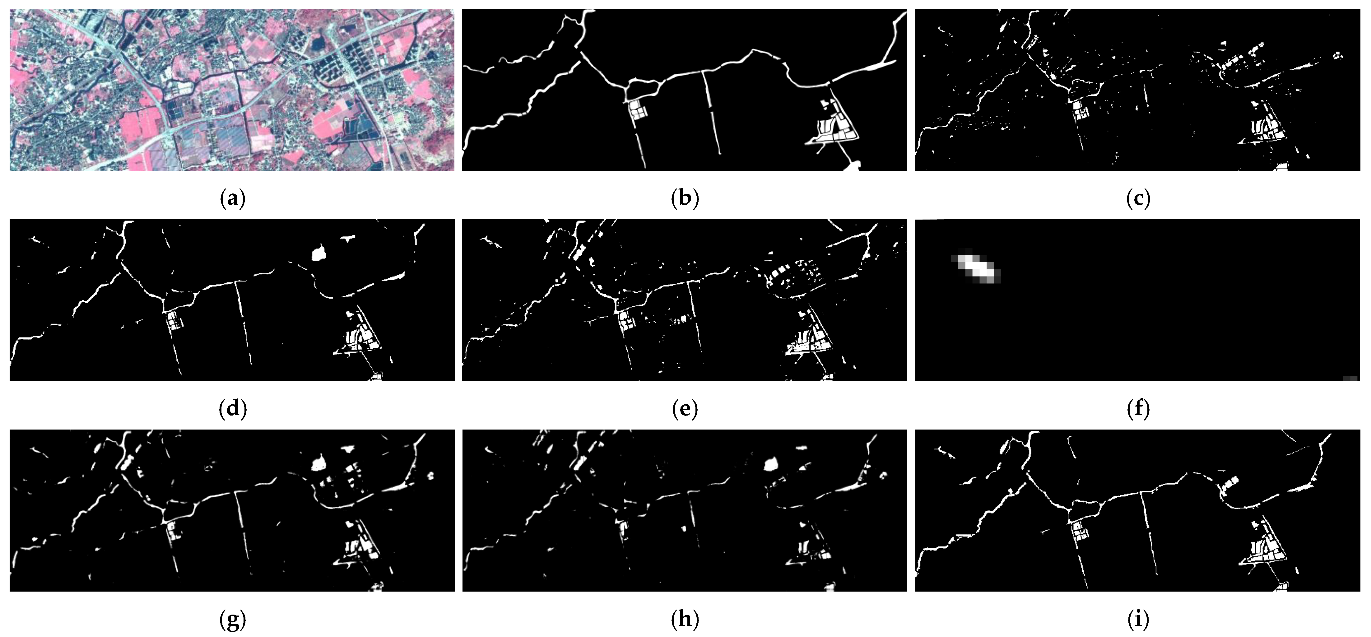
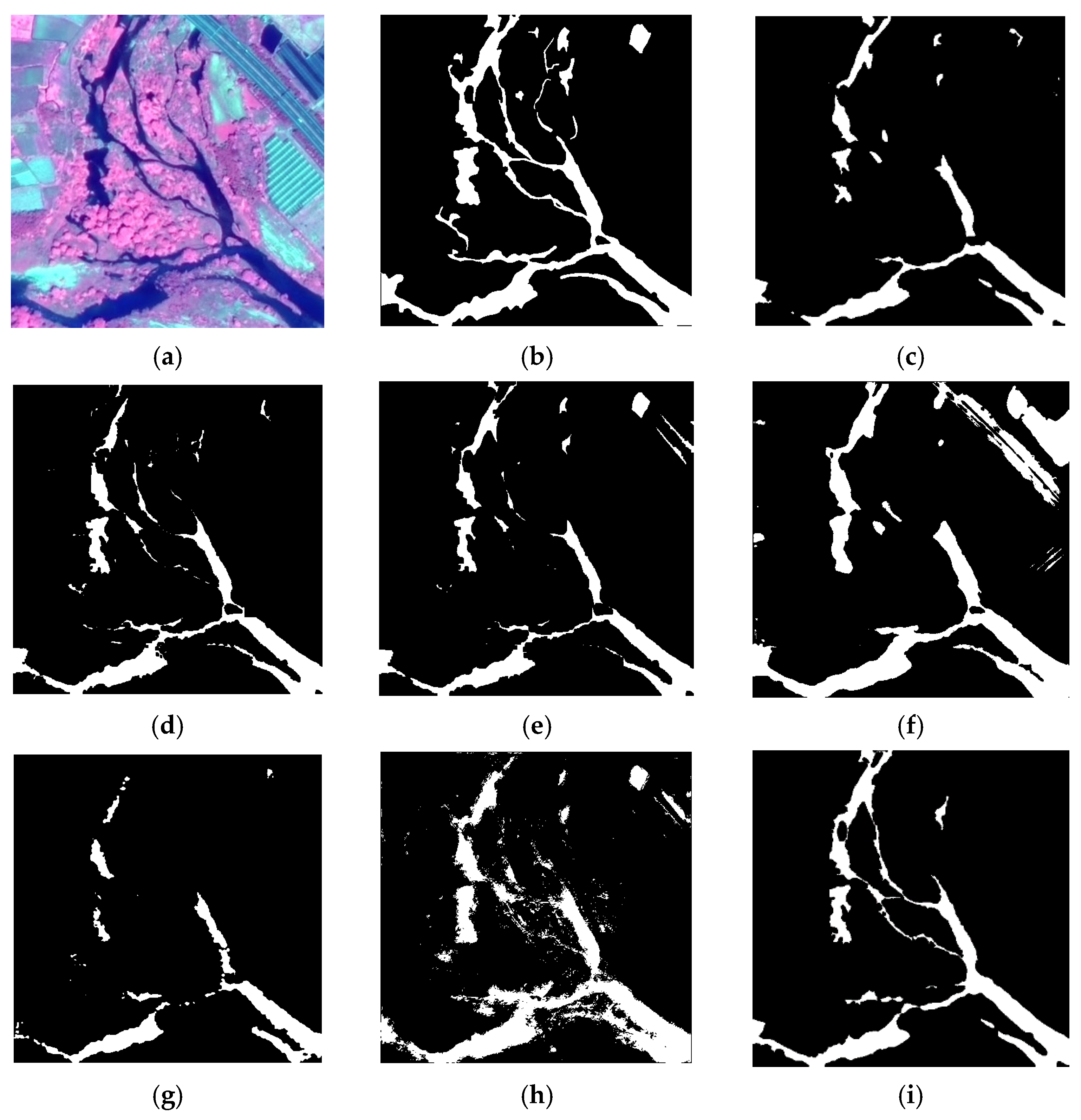
4.3. Comparative Experiment Analysis

In order to test the effectiveness of the proposed method, five methods are compared. First, small water optimization [64] and SVM classification [65] are selected as traditional comparative methods, while MSResNet [66], MFGF_U-Net [67] and MECNet [68] are compared as deep learning-based methods. Small water extraction [64] proposes using multi-scale and spectral difference segmentation to extract large water bodies and proposes an object-oriented water index Brightness Green ratio BGR for small water bodies. SVM classification [65] uses the SVM algorithm, which is known for its high classification accuracy, is highly robust to noise, and capable of handling complex water distributions. Its flexibility allows it to adapt to various data types, making it particularly effective in diverse water environments. MSResNet [66] enhances water detection by leveraging multi-scale residual convolution (MSDC) for capturing global context through global average pooling (GAP) and dimensionality reduction, while multi-scale feature fusion (MKMP) preserves and refines structural details through upsampling and feature stitching. The integration of these modules enables effective multi-scale feature extraction, significantly improving water body differentiation and detection accuracy. MFGF_U-Net [67] utilizes a U-shaped encoder–decoder structure with ConvBR blocks and upsampling to efficiently extract and restore feature maps. To handle water bodies of varying sizes and shapes, it integrates a gated multi-filter inception (GMF-Inception) module and an attention mechanism, leveraging multi-modal information for improved segmentation accuracy, robustness, and computational efficiency. MECNet [68] uses a multi-feature extraction and combination module, incorporates a multi-scale prediction fusion module for fine contour detection, and employs an encoder–decoder semantic feature fusion module to enhance feature consistency, achieving water extraction.

To prove the effectiveness and robustness of the proposed method, a high-resolution remote sensing image was selected for experimental analysis, and the image was recorded as S1, as shown in Figure 4a, Figure 5a, Figure 6a and Figure 7a. The ground truth labels are shown in Figure 4b, Figure 5b, Figure 6b and Figure 7b. There are various types of objects, such as buildings, lakes, woodlands, farmlands, and roads. In this paper, we designed an U-Net-based network which is used to extract the initial water body from high resolution images. After preliminary processing, the extraction result is used as the initial result, as shown in Figure 4c, Figure 5c, Figure 6c and Figure 7c. The comparative results are shown in Figure 4d–h, Figure 5d–h, Figure 6d–h and Figure 7d–h. The accuracy comparison results of the three methods are shown in

Table 1. Comparison of accuracy of water optimization results of image S1.

Method	CR/%	CM/%	F1/%	OA/%
Initial result	85.53	56.65	68.15	97.73
Small water optimization	62.67	41.25	49.75	96.43
SVM classification	60.67	62.56	56.35	96.50
MFGF_U-Net	51.56	49.12	50.31	95.84
MSResNet	67.95	55.00	60.80	96.96
MECNet	66.86	35.47	46.35	96.48
Ours	75.39	71.78	73.54	98.65

,

Table 2. Comparison of accuracy of water optimization results of image S2.

Method	CR/%	CM/%	F1/%	OA/%
Initial result	98.22	54.52	70.12	93.19
Small water optimization	98.63	61.47	75.74	94.23
SVM classification	97.03	55.04	70.24	93.17
MFGF_U-Net	67.29	76.23	71.48	91.09
MSResNet	98.94	41.24	58.22	91.33
MECNet	72.10	73.63	72.86	91.96
Ours	95.71	69.13	80.27	95.02

,

Table 3. Comparison of accuracy of water optimization results of image S3.

Method	CR/%	CM/%	F1/%	OA/%
Initial result	97.32	59.23	73.64	97.16
Small water optimization	68.85	62.11	65.31	95.59
SVM classification	76.74	58.99	66.70	96.06
MFGF_U-Net	47.04	93.97	62.69	92.52
MSResNet	91.57	58.24	71.20	96.85
MECNet	98.18	51.53	67.59	96.69
Ours	81.98	84.94	83.43	97.74

and

Table 4. Comparison of accuracy of water optimization results of image S4.

Method	CR/%	CM/%	F1/%	OA/%
Initial result	99.65	48.39	65.14	85.30
Small water optimization	99.55	66.47	79.71	90.39
SVM classification	99.99	49.98	66.65	85.80
MFGF_U-Net	88.40	67.97	76.85	88.37
MSResNet	99.81	22.89	37.24	78.09
MECNet	75.01	68.79	71.76	84.63
Ours	97.55	75.24	84.95	92.43

. Our proposed method is shown in Figure 4f, Figure 5f, Figure 6f and Figure 7f.

Small water optimization is mainly designed to optimize the interference of shadows in the identification of small water bodies. As shown in Figure 4d, Figure 5d, Figure 6d and Figure 7d, there is a clear optimization effect when eliminating erroneous results between small water bodies and shadows, such as shown in image S1. However, the ability to distinguish shadows in some large areas is unstable, such as in S3. The results of this optimization method for large-area water bodies still depend on the extraction effect of the initial results. For example, in image S2, the effect of supplementing the insufficient water extraction in the original result is weak.

The SVM classification method combines spectral and shape texture information to construct a water body classifier. As shown in Figure 4e, Figure 5e, Figure 6e and Figure 7e, the SVM classification method can extract bright water bodies while, at the same time, extracting dark water bodies. However, one disadvantage of this approach is that, since roads and shadows have similar spectral features as the selected samples, to varying degrees, they will be mistakenly identified as water bodies when using SVM classification. In addition, for small water bodies, the recognition effect of using the SVM classification method is not stable enough. When the spectra of such small water bodies are similar, they can be identified completely. In addition, when the water depth of a small river is shallow and the spectral feature differences vary greatly, it is very easy to make detection errors. As shown in Figure 4, Figure 5, Figure 6 and Figure 7, there is still a phenomenon of interruption of water flow.

MFGF_U-Net is designed on the basis of U-Net and improved to optimize computational efficiency. This method integrates the stability of U-Net, and the results of water body detection are basically stable. However, when there are roads and shadows in the urban area, there will be a lot of misjudgments.

MSResNet adopts a multi-scale residual convolution network to extract water bodies. The residual network is not as stable as U-Net in the segmentation network structure. The stability of this method in water body extraction results in different scenes is relatively poor. For example, in image S1, MSResNet achieved results that were second only to the method used in this paper. However, the effect of water body recognition in image S4 is relatively weaker.

MECNet is a CNN network model based on the encoder–decoder structure. It emphasizes the optimization of multi-scale convolution and prediction modules. When used for water body extraction, it has a strong ability to capture details. For example, in images S2 and S4, the extraction of large water bodies is relatively complete. However, some of the surrounding interfering objects will also be identified as water bodies, resulting in a decrease in recognition accuracy. This type of method still has a weak ability to identify and process small water bodies, making it difficult to extract rivers completely.

Our proposed method as shown in Figure 4f, Figure 5f, Figure 6f and Figure 7f, uses Frangi filtering to extract small tributaries. The local SSIM index and the interoperability algorithm connect the broken parts in the small tributaries, and can extract the small rivers, supplement the lack of small water bodies and correct the problem of broken flow. Moreover, it realizes the accurate optimization of the linear tributaries and achieves better optimization results. As shown in image S1, our initial results based on this network achieved second place among all the results. The long and fine river is also discontinuous. After our improvement, the final result is better. The river is connected and many wrong detections are removed. Compared with the initial extraction results, the accuracy of our optimized results increased by 0.92% on OA, 5.39% on F1 score, and 15.13% on CM. The average F1 and OA of our final results are higher than those produced by other methods by 25% and 2%, respectively. As shown in image S2, There are many branching tributaries in this big river, forming a tree-like network structure. There are many missed detections in the initial detection results of this paper. Through the optimization method of this paper, these missed water bodies are supplemented more completely. The main function is to rely on the nonlinear water body optimization part to supplement the water bodies with similar spectra. Compared with the initial extraction results, the optimized water body results increased by 10.15 on F1 and 1.83 on OA. The final result is also better than that of all the other comparison methods. The average F1 and OA are higher by 8% and 3%, respectively. Image S3 includes a neatly shaped river that runs through the middle of the city, with little variation in river width. The initial results did not detect the entire river, and there was an obvious interruption in it. After optimizing and supplementing the interruption of linear water bodies using the method in this paper, the optimized water results increased by 0.58% on OA, 9.79% on F1 score, and 25.71% on CM compared to the initial results. Compared with the other methods, the average accuracy of the optimized water body results is 15% better on F1 and 2% on OA. With regard toS4, the initial results also contain numerous instances of misclassification. By optimizing and supplementing the missed water body detections, the initial results of our optimized water results increased the precision of OA by 7.13%, F1 score by 19.81%, and CM by 26.85%. Compared with the other optimization methods, our average accuracy is increased by 20% on F1 and 8% on OA. The accuracy comparison results show that the proposed method can improve the integrity and regularity of water body results, and the comprehensive value and overall accuracy are better than the initial extraction results.

To visually show the differences between different methods, this paper selects five single river images for comparison, as shown in Figure 8. From top to bottom, there are five river regions named #1, #2, #3, #4 and #5. These rivers are fine, and the surrounding features are different. As shown in #3 and #4, the results of small water optimization in Figure 8c are relatively incomplete for extracting the river. Since the initial result is obtained based on water indices, sometimes this method cannot detect water as the spectrum threshold is used inaccurately, such as in #2 and #4. Especially if there is abundant noise near the river, there will be more misclassification after optimization, as shown in #3. SVM classification is not able to detect the fine river completely. As demonstrated for #2 and #4, the river is detected with inaccurate width. The results of MFGF_U-Net are relatively more complete than those of the other methods. However, there are also some wrong detections, such as #1 in Figure 8e. MSResNet is weaker than the other two deep learning methods. The missing river problem is more serious than in other methods, as shown in #2–#4. The result of MECNet, in Figure 8g, is relatively more complete. However, when the shape of the road and the river are wide and narrow and the texture features are similar, errors will occur, such as in #2. When the river is thinner and more curved, there will be a lack of fragments, as shown in #1. Compared with the other methods, the optimization results of this paper (Figure 8h) connect the missing parts of the fragment, making the river more complete. This is achieved through the final optimization, so that the final result is closer to the real shape of the water. In terms of accuracy evaluation, Figure 9 shows the accuracy comparison of each single river optimization in Figure 8. The overall accuracy of the river optimized by our method demonstrates much better improvement, compared with the five reference methods.

Our method addresses the issue of missing river fragments and the lack of small rivers in water extraction from high-resolution remote sensing images. By using Frangi filtering, the GA-OTSU threshold segmentation algorithm, and a discontinuous connection algorithm, linear tributaries in the image are extracted, and discontinuities in the river are effectively connected. The final optimization step allows for the supplementation of small water bodies. Water bodies are extracted using K-means clustering, and small area misclassifications are removed through morphological operations. As a result, the proposed method outperforms others, aligns well with the actual water body structure, and demonstrates strong generalizability.

4.4. Ablation Experiment

To assess the effectiveness and contribution of each optimization module—Preliminary Optimization (PO), Depth Optimization (DO), and Nonlinear Optimization (NO)—in the proposed method, this study conducted ablation experiments. By sequentially modifying different components of the method and evaluating their impact on overall performance, the importance of each module in achieving the final results was determined. In this experiment, the ablation analysis primarily focused on the following components of the model. The PO module includes the Frangi filter and GA-OTSU. The DO module consists of river skeleton refinement extraction and broken part connection. The NO module is responsible for spectrum inspection, which effectively removes small non-water regions.

Table 5. Ablation experiment results.

Modules	CR/%	CM/%	F1/%	OA/%
Initial results	65.91	91.71	76.70	96.88
PO	90.83	92.15	90.42	97.57
PO + DO	94.95	93.71	92.30	98.41
PO + DO + NO	97.92	95.38	96.64	99.46

shows the water detection results using different modules. After incorporating the PO module, accuracy is significantly improved, indicating that the GA-OTSU module plays a crucial role in enhancing both the accuracy and stability of the model. The addition of the DO module further boosts accuracy. By subsequently adding the NO module, misclassified non-water regions, particularly small nonlinear ones, are eliminated. The ablation experiment demonstrates that each module in our approach contributes uniquely to the overall performance. Notably, the DO module has a substantial impact on improving extraction accuracy. The effective combination of these modules results in a substantial enhancement of the initial outcomes.

5. Discussion

5.1. Effectiveness Analysis of Preliminary Optimization

To verify the effectiveness of the proposed algorithm in the preliminary optimization of rivers, image S5 in Figure 10 and Figure 11 are selected for comparison. Figure 10b and Figure 11b show the initial water extraction results. The water body is preliminarily extracted by combining the Frangi filtering algorithm and the GA-OTSU segmentation algorithm. The results are shown in Figure 10c and Figure 11c. Compared with the initial extraction result, the optimized results are more detailed and complete. In comparison, it can be seen that the preliminary optimization algorithm can not only identify a finer, meandering river but also capture small tributaries. This improvement not only complements the lack of details in the initial extraction results but also improves the integrity of water extraction as a whole. In general, the river preliminary extraction algorithm extracts more rivers by the linear water body preliminary extraction method based on global features, which supplements the lack of small water bodies and obtains a more complete water body.

5.2. Effectiveness Analysis of Depth Optimization Algorithm

To verify the effectiveness of the depth optimization algorithm, S7–S9 are selected in Figure 12, Figure 13 and Figure 14. During the depth optimization process, a disconnection continuation algorithm is applied to optimize the high-resolution remote sensing images. This algorithm detects river breakpoints by extracting the water skeleton and precisely identifying discontinuities in the river. These breakpoints are crucial for addressing river discontinuities. Next, the algorithm computes the circumscribed rectangle surrounding the potential flow-breaking regions and the corresponding influence subgraphs. Based on this information, the algorithm performs fine connection operations to bridge the discontinuous river segments. Through a series of complex calculations and decisions, the algorithm successfully reconnects the previously fragmented river sections, transforming the river into a continuous and coherent water body. The results, presented in Figure 12d, Figure 13d and Figure 14d, show a marked improvement compared to the initial extraction shown in Figure 12c, Figure 13c and Figure 14c, and the water basin is more complete. The algorithm effectively addresses river cutoffs, yielding more continuous water results.

6. Conclusions

In this paper, a river connection optimization method as part of high-resolution remote sensing images is proposed. This method focuses on the preliminary optimization of linear water bodies and the disconnection problem in water body extraction to conduct in depth optimization, in order to improve the accuracy and integrity of water body extraction results. To effectively solve the problem of false detection and missed detection of fine and small rivers in the initial results, this paper proposes a new linear feature preliminary optimization method. Firstly, the global features of high resolution remote sensing images are extracted by the Frangi filter, to significantly enhance the linear feature response in the image in order to accurately identify the linear river; this effectively supplements the initial results of the river obtained by the classification method, to obtain the preliminary optimized river information. To address the problems of discontinuous rivers in the preliminary optimization results, this paper proposes a depth discontinuous river connection optimization method, which combines the local connected domain labeling algorithm and SSIM index to connect the discontinuous river parts. Finally, to further inspect the nonlinear water information, K-means clustering and spectral–morphological joint inspection are used to supplement the large water area with holes, remove noise interference, and optimize the details of the water. Experiments show that the proposed method can effectively connect disconnected rivers, improve the problem of discontinuous optimization, and further improve the accuracy of optimization.

In the future, in-depth time series information analysis will be carried out in combination with time series remote sensing image data to monitor and analyze the seasonal and periodic changes of water bodies. This will help to better understand the dynamic changes of water bodies and provide a more in-depth reference for water resource management and environmental protection.

References

1. Yang, D.; Gao, X.; Yang, Y.; Guo, K.; Han, K.; Xu, L. Advances and Future Prospects in Building Extraction from High-Resolution Remote Sensing Images. IEEE J. Sel. Top. Appl. Earth Obs. Remote Sens. 2025, 1–25. [Google Scholar] [CrossRef]
2. Gao, X.; Zhang, G.; Yang, Y.; Kuang, J.; Han, K.; Jiang, M.; Yang, J.; Tan, M.; Liu, B. Two-Stage Domain Adaptation Based on Image and Feature Levels for Cloud Detection in Cross-Spatiotemporal Domain. IEEE Trans. Geosci. Remote Sens. 2024, 62, 5610517. [Google Scholar] [CrossRef]
3. Zhang, G.; Gao, X.; Yang, J.; Yang, Y.; Tan, M.; Xu, J.; Wang, Y. A multi-task driven and reconfigurable network for cloud detection in cloud-snow coexistence regions from very-high-resolution remote sensing images. Int. J. Appl. Earth Obs. Geoinf. 2022, 114, 103070. [Google Scholar] [CrossRef]
4. Topp, S.N.; Pavelsky, T.M.; Jensen, D.; Simard, M.; Ross, M.R.V. Research Trends in the Use of Remote Sensing for Inland Water Quality Science: Moving Towards Multidisciplinary Applications. Water 2020, 12, 169. [Google Scholar] [CrossRef]
5. Liu, Z.; Gao, X.; Yang, Y.; Xu, L.; Wang, S.; Chen, N.; Wang, Z.; Kou, Y. EDT-Net: A Lightweight Tunnel Water Leakage Detection Network Based on LiDAR Point Clouds Intensity Images. IEEE J. Sel. Top. Appl. Earth Obs. Remote Sens. 2025, 1–13. [Google Scholar] [CrossRef]
6. Xu, T.; Gao, X.; Yang, Y.; Xu, L.; Xu, J.; Wang, Y. Construction of a Semantic Segmentation Network for the Overhead Catenary System Point Cloud Based on Multi-Scale Feature Fusion. Remote Sens. 2022, 14, 2768. [Google Scholar] [CrossRef]
7. Cracknell, A.P. The development of remote sensing in the last 40 years. Int. J. Remote Sens. 2018, 39, 8387–8427. [Google Scholar] [CrossRef]
8. Yang, C.; Wei, Y.; Wang, S.; Zhang, Z.; Huang, S. Extracting the flood extent from satellite SAR image with the support of topographic data. In Proceedings of the 2001 International Conferences on Info-Tech and Info-Net, Beijing, China, 29 October–1 November 2001; pp. 87–92. [Google Scholar]
9. Chen, J.; Chen, S.; Fu, R.; Li, D.; Jiang, H.; Wang, C.; Peng, Y.; Jia, K.; Hicks, B.J. Remote sensing big data for water environment monitoring: Current status, challenges, and future prospects. Earth’s Future 2022, 10, e2021EF002289. [Google Scholar] [CrossRef]
10. Cheng, C.; Zhang, F.; Shi, J.; Kung, H.-T. What is the relationship between land use and surface water quality? A review and prospects from remote sensing perspective. Environ. Sci. Pollut. Res. 2022, 29, 56887–56907. [Google Scholar] [CrossRef]
11. Wu, P.; Fu, J.; Yi, X.; Wang, G.; Mo, L.; Maponde, B.T.; Liang, H.; Tao, C.; Ge, W.; Jiang, T. Research on water extraction from high resolution remote sensing images based on deep learning. Front. Remote Sens. 2023, 4, 1283615. [Google Scholar] [CrossRef]
12. Li, M.; Wu, P.; Wang, B.; Park, H.; Hui, Y.; Wu, Y. A Deep Learning Method of Water Body Extraction from High Resolution Remote Sensing Images with Multisensors. IEEE J. Sel. Top. Appl. Earth Obs. Remote Sens. 2021, 14, 3120–3132. [Google Scholar] [CrossRef]
13. Zhang, Y.; Yang, Y.; Gao, X.; Xu, L.; Liu, B.; Liang, X. Robust Extraction of Multiple-Type Support Positioning Devices in the Catenary System of Railway Dataset Based on MLS Point Clouds. IEEE Trans. Geosci. Remote Sens. 2023, 61, 5702314. [Google Scholar] [CrossRef]
14. Wu, B.; Gao, Y.; Xie, X.; Yang, Y. Research and Application of Automatic Recognition and Extraction of Water Body in Remote Sensing Images Based on Deep Learning. In Wireless Technology, Intelligent Network Technologies, Smart Services and Applications. Smart Innovation, Systems and Technologies; Springer: Singapore, 2022. [Google Scholar]
15. Qi, B.; Zhuang, Y.; Chen, H.; Dong, S.; Li, L. Fusion Feature Multi-Scale Pooling for Water Body Extraction from Optical Panchromatic Images. Remote Sens. 2019, 11, 245. [Google Scholar] [CrossRef]
16. Kang, J.; Guan, H.; Li, X.J. WaterFormer: A coupled transformer and CNN network for waterbody detection in optical remotely-sensed imagery. ISPRS J. Photogramm. Remote Sens. 2023, 206, 222–241. [Google Scholar] [CrossRef]
17. Chen, B.; Huang, B.; Xu, B. Multi-source remotely sensed data fusion for improving land cover classification. ISPRS J. Photogramm. Remote Sens. 2017, 124, 27–39. [Google Scholar] [CrossRef]
18. Sun, D.; Gao, G.; Huang, L.; Liu, Y.; Liu, D. Extraction of water bodies from high-resolution remote sensing imagery based on a deep semantic segmentation network. Sci. Rep. 2024, 14, 14604. [Google Scholar] [CrossRef]
19. Cheng, X.; Han, K.; Xu, J.; Li, G.; Xiao, X.; Zhao, W.; Gao, X. SPFDNet: Water Extraction Method Based on Spatial Partition and Feature Decoupling. Remote Sens. 2024, 16, 3959. [Google Scholar] [CrossRef]
20. Nath, R.K.; Deb, S.K. Water-Body Area Extraction from High Resolution Satellite Images-An Introduction, Review, and Comparison. Int. J. Image Process. 2010, 3, 353–372. [Google Scholar]
21. Zhu, Y.; Sun, L.J.; Zhang, C.Y. Summary of water body extraction methods based on ZY-3 satellite. In Proceedings of the Iop Conference Series: Earth & Environmental Science, Shanghai, China, 19–22 October 2017. [Google Scholar]
22. Chen, C.; Liang, J.; Chen, Z.J. Method of Water Body Information Extraction in Complex Geographical Environment from Remote Sensing Images. Sens. Mater. Int. J. Sens. Technol. 2022, 34, 4325–4338. [Google Scholar] [CrossRef]
23. Li, J.; Meng, Y.; Li, Y.; Cui, Q.; Yang, X.; Tao, C.; Wang, Z.; Li, L.; Zhang, W. Accurate water extraction using remote sensing imagery based on normalized difference water index and unsupervised deep learning. J. Hydrol. 2022, 612, 128202. [Google Scholar] [CrossRef]
24. Liu, C.; Tang, H.; Ji, L.; Zhao, Y. Spatial-temporal water area monitoring of Miyun Reservoir using remote sensing imagery from 1984 to 2020. arXiv 2021, arXiv:2110.09515. [Google Scholar] [CrossRef]
25. Maulik, U.; Chakraborty, D. Remote Sensing Image Classification: A survey of support-vector-machine-based advanced techniques. IEEE Geosci. Remote Sens. Mag. 2017, 5, 33–52. [Google Scholar] [CrossRef]
26. Sheykhmousa, M.; Mahdianpari, M.; Ghanbari, H.; Mohammadimanesh, F.; Ghamisi, P.; Homayouni, S. Support Vector Machine Versus Random Forest for Remote Sensing Image Classification: A Meta-Analysis and Systematic Review. IEEE J. Sel. Top. Appl. Earth Obs. Remote Sens. 2020, 13, 6308–6325. [Google Scholar] [CrossRef]
27. Gao, X.; Wang, M.; Yang, Y.; Li, G. Building Extraction From RGB VHR Images Using Shifted Shadow Algorithm. IEEE Access 2018, 6, 22034–22045. [Google Scholar] [CrossRef]
28. Cao, H.; Tian, Y.; Liu, Y.; Wang, R. Water body extraction from high spatial resolution remote sensing images based on enhanced U-Net and multi-scale information fusion. Sci. Rep. 2024, 14, 16132. [Google Scholar] [CrossRef]
29. Acharya, T.D.; Subedi, A.; Lee, D.H. Evaluation of machine learning algorithms for surface water extraction in a Landsat 8 scene of Nepal. Sensors 2019, 19, 2769. [Google Scholar] [CrossRef]
30. Hu, W. Urban Water Extraction with UAV High-Resolution Remote Sensing Data Based on an Improved U-Net Model. Remote Sens. 2021, 13, 3165. [Google Scholar] [CrossRef]
31. Chen, Y.; Fan, R.S.; Yang, X.C.; Wang, J.X.; Latif, A. Extraction of Urban Water Bodies from High-Resolution Remote-Sensing Imagery Using Deep Learning. Water 2018, 10, 585. [Google Scholar] [CrossRef]
32. Georganos, S.; Grippa, T.; Vanhuysse, S.; Lennert, M.; Shimoni, M.; Kalogirou, S.; Wolff, E. Less is more: Optimizing classification performance through feature selection in a very-high-resolution remote sensing object-based urban application. Giscience Remote Sens. 2017, 55, 221–242. [Google Scholar] [CrossRef]
33. Li, J.; Cheng, K.; Wang, S.; Morstatter, F.; Trevino, R.P.; Tang, J.; Liu, H. Feature Selection: A Data Perspective. Acm Comput. Surv. 2016, 50, 94. [Google Scholar] [CrossRef]
34. Rad, A.M.; Kreitler, J.; Sadegh, M. Augmented Normalized Difference Water Index for improved surface water monitoring. Environ. Model. Softw. 2021, 140, 105030. [Google Scholar] [CrossRef]
35. Zhang, T.; Ji, W.; Li, W.; Qin, C.; Wang, T.; Ren, Y.; Fang, Y.; Han, Z.; Jiao, L. EDWNet: A Novel Encoder–Decoder Architecture Network for Water Body Extraction from Optical Images. Remote Sens. 2024, 16, 4275. [Google Scholar] [CrossRef]
36. Zhu, X.X.; Tuia, D.; Mou, L.; Xia, G.S.; Zhang, L.; Xu, F.; Fraundorfer, F. Deep Learning in Remote Sensing: A Comprehensive Review and List of Resources. IEEE Geosci. Remote Sens. Mag. 2018, 5, 8–36. [Google Scholar] [CrossRef]
37. Liu, T.; Yuan, M.; Lu, C.; Lu, K.; Peng, B.; Duan, H.; Li, M.; Zhang, P.; Wang, T.; Liao, T. Water Body Extraction from SAR and Multi-Source Data Using Siamese Network-Based Segmentation. In Proceedings of the IGARSS 2024-2024 IEEE International Geoscience and Remote Sensing Symposium, Athens, Greece, 7–12 July 2024; pp. 772–775. [Google Scholar]
38. Shuangtong, L.; Ming-Xiao, W.; Shuwen, Y.; Mingze, Y.; Lihua, Y. Extraction accuracy and stability analysis of different water body index models in GF-2 images. Bull. Surv. Mapp. 2019, 8, 135. [Google Scholar]
39. Lan, L.; Wang, Y.G.; Chen, H.S.; Gao, X.R.; Wang, X.K.; Yan, X.F. Improving on mapping long-term surface water with a novel framework based on the Landsat imagery series. J. Environ. Manag. 2024, 353, 120202. [Google Scholar] [CrossRef]
40. Wang, Z.; Liu, J.; Li, J.; Zhang, D.D. Multi-Spectral Water Index (MuWI): A Native 10-m Multi-Spectral Water Index for Accurate Water Mapping on Sentinel-2. Remote Sens. 2018, 10, 1643. [Google Scholar] [CrossRef]
41. Fang-Fang, Z.; Bing, Z.; Jun-Sheng, L.; Qian, S.; Yuanfeng, W.; Yang, S. Comparative Analysis of Automatic Water Identification Method Based on Multispectral Remote Sensing. Procedia Environ. Sci. 2011, 11, 1482–1487. [Google Scholar] [CrossRef]
42. Zhang, W.; Zhao, L. The Track, Hotspot and Frontier of International Hyperspectral remote sensing Research 2009–2019—A Bibliometric Analysis Based on SCI Database. Measurement 2021, 187, 110229. [Google Scholar] [CrossRef]
43. Kurban, T. Region based multi-spectral fusion method for remote sensing images using differential search algorithm and IHS transform. Expert Syst. Appl. 2022, 189, 116135. [Google Scholar] [CrossRef]
44. Yan, Y.; Yu, W.; Zhang, L. A method of band selection of remote sensing image based on clustering and intra-class index. Multimed. Tools Appl. 2022, 81, 22111–22128. [Google Scholar] [CrossRef]
45. Zhao, B.; Wu, J.; Han, X.; Tian, F.; Liu, M.; Chen, M.; Lin, J. An improved surface water extraction method by integrating multi-type priori information from remote sensing. Int. J. Appl. Earth Obs. Geoinf. 2023, 124, 103529. [Google Scholar] [CrossRef]
46. Ma, L.; Li, M.; Ma, X.; Cheng, L.; Du, P.; Liu, Y. A review of supervised object-based land-cover image classification. ISPRS J. Photogramm. Remote Sens. 2017, 130, 277–293. [Google Scholar] [CrossRef]
47. Lang, S. Object-based image analysis for remote sensing applications: Modeling reality—Dealing with complexity. In Object-Based Image Analysis; Springer: Berlin/Heidelberg, Germany, 2008. [Google Scholar]
48. Zhang, X.; Zhang, T.; Jiao, J.L. Remote Sensing Object Detection Meets Deep Learning: A metareview of challenges and advances. Geosci. Remote Sens. 2023, 11, 8–44. [Google Scholar] [CrossRef]
49. Paul, A.; Tripathi, D.; Dutta, D. Application and comparison of advanced supervised classifiers in extraction of water bodies from remote sensing images. Sustain. Water Resour. Manag. 2018, 4, 905–919. [Google Scholar] [CrossRef]
50. Xue, Y.; Qin, C.; Baosheng, W.U.; Dan, L.I.; Xudong, F.U. Automatic extraction of mountain river information from multiple Chinese high-resolution remote sensing satellite images. J. Tsinghua Univ. (Sci. Technol.) 2023, 63, 134–145. [Google Scholar]
51. Sharma, R.; Ghosh, A.; Joshi, P.K. Analysing spatio-temporal footprints of urbanization on environment of Surat city using satellite-derived bio-physical parameters. Geocarto Int. 2012, 28, 420–438. [Google Scholar] [CrossRef]
52. Shaowei, W.; Xiaoxiang, Z.; Xiaoying, Y. Land Use Classification based on Remote Sensing Image in Taihu Lake Lakeside Sensitive Area. Remote Sens. Technol. Appl. 2014, 29, 114–121. [Google Scholar]
53. Blaschke, T. Object based image analysis for remote sensing. ISPRS J. Photogramm. Remote Sens. 2010, 65, 2–16. [Google Scholar] [CrossRef]
54. Xu, J. Optimization of Remote-Sensing Image-Segmentation Decoder Based on Multi-Dilation and Large-Kernel Convolution. Remote Sens. 2024, 16, 2851. [Google Scholar] [CrossRef]
55. Li, E.; Samat, A.; Du, P.; Liu, W.; Hu, J. Improved Bilinear CNN Model for Remote Sensing Scene Classification. IEEE Geosci. Remote Sens. Lett. 2020, 19, 8004305. [Google Scholar] [CrossRef]
56. Pan, J.; Wei, Z.; Zhao, Y.; Zhou, Y.; Lin, X.; Zhang, W.; Tang, C. Enhanced FCN for farmland extraction from remote sensing image. Multimed. Tools Appl. 2022, 81, 38123–38150. [Google Scholar] [CrossRef]
57. Yu, Y.; Yao, Y.; Guan, H.; Li, D.; Liu, Z.; Wang, L.; Yu, C.; Xiao, S.; Wang, W.; Chang, L. A self-attention capsule feature pyramid network for water body extraction from remote sensing imagery. Int. J. Remote Sens. 2021, 42, 1801–1822. [Google Scholar] [CrossRef]
58. Chen, L.C.; Papandreou, G.; Kokkinos, I.; Murphy, K.; Yuille, A.L. DeepLab: Semantic Image Segmentation with Deep Convolutional Nets, Atrous Convolution, and Fully Connected CRFs. IEEE Trans. Pattern Anal. Mach. Intell. 2018, 40, 834–848. [Google Scholar] [CrossRef]
59. Wu, B.; Zhang, J.; Zhao, Y. A Novel Method to Extract Narrow Water Using a Top-Hat White Transform Enhancement Technique. J. Indian Soc. Remote Sens. 2019, 47, 391–400. [Google Scholar] [CrossRef]
60. Kang, J.; Guan, H.; Peng, D.; Chen, Z. Multi-scale context extractor network for water-body extraction from high-resolution optical remotely sensed images. Int. J. Appl. Earth Obs. Geoinf. 2021, 103, 102499. [Google Scholar] [CrossRef]
61. Horé, A.; Ziou, D. Image quality metrics: PSNR vs. SSIM. In Proceedings of the 20th International Conference on Pattern Recognition, ICPR 2010, Istanbul, Turkey, 23–26 August 2010. [Google Scholar]
62. Xu, Y.; Lin, J.; Zhao, J.; Zhu, X. New method improves extraction accuracy of lake water bodies in Central Asia. J. Hydrol. 2021, 603, 127180. [Google Scholar] [CrossRef]
63. Tong, X.-Y.; Xia, G.-S.; Lu, Q.; Shen, H.; Li, S.; You, S.; Zhang, L. Land-cover classification with high-resolution remote sensing images using transferable deep models. Remote Sens. Environ. 2020, 237, 111322. [Google Scholar] [CrossRef]
64. Chen, R.; Pu, Y.; Zhou, J.; Li, J.; Wang, X. Small Water Body Extraction Based on GF-2 Image. Laser Optoelectron. Prog. 2023, 60, 1628002. [Google Scholar]
65. Li, L.; Wu, K.; Zhou, D.-W. Extraction algorithm of mining subsidence information on water area based on support vector machine. Environ. Earth Sci. 2014, 72, 3991–4000. [Google Scholar] [CrossRef]
66. Dang, B.; Li, Y. MSResNet: Multiscale residual network via self-supervised learning for water-body detection in remote sensing imagery. Remote Sens. 2021, 13, 3122. [Google Scholar] [CrossRef]
67. Wang, R.; Zhang, C.; Chen, C.; Hao, H.; Li, W.; Jiao, L. A Multi-Modality Fusion and Gated Multi-Filter U-Net for Water Area Segmentation in Remote Sensing. Remote Sens. 2024, 16, 419. [Google Scholar] [CrossRef]
68. Zhang, Z.; Lu, M.; Ji, S.; Yu, H.; Nie, C. Rich CNN features for water-body segmentation from very high resolution aerial and satellite imagery. Remote Sens. 2021, 13, 1912. [Google Scholar] [CrossRef]
Figure 1. Flow chart of water body optimization.
Remotesensing 17 00742 g001
Figure 2. Thinning and extracting skeleton endpoint schematic diagram. (a) Preliminary river results of flow-breaks. (b) Refining the skeleton endpoints.
Remotesensing 17 00742 g002
Figure 3. Schematic diagram of the connected domain tagging algorithm. (a) Water extraction results. (b) Labeling results. 1–3 represent different water pixels group with different labels.
Remotesensing 17 00742 g003
Figure 4. Comparison of water optimization results of image S1. (a) Image S1, (b) Ground truth, (c) Initial results, (d) Small water optimization, (e) SVM classification, (f) MFGF_U-Net, (g) MSResNet, (h) MECNet (i) Ours. White pixel represents water. Black pixels represents non-water.
Remotesensing 17 00742 g004
Figure 5. Comparison of water optimization results of image S2. (a) Image S2, (b) Ground truth, (c) Initial results, (d) Small water optimization, (e) SVM classification, (f) MFGF_U-Net, (g) MSResNet, (h) MECNet (i) Ours. White pixel represents water. Black pixels represents non-water.
Remotesensing 17 00742 g005
Figure 6. Comparison of water optimization results of image S3. (a) Image S3, (b) Ground truth, (c) Initial results, (d) Small water optimization, (e) SVM classification, (f) MFGF_U-Net, (g) MSResNet, (h) MECNet, (i) Ours. White pixel represents water. Black pixels represents non-water.
Remotesensing 17 00742 g006aRemotesensing 17 00742 g006b
Figure 7. Comparison of water optimization results of image S4. (a) Image S4, (b) Ground truth, (c) Initial results, (d) Small water optimization, (e) SVM classification, (f) MFGF_U-Net, (g) MSResNet, (h) MECNet (i) Ours. White pixel represents water. Black pixels represents non-water.
Remotesensing 17 00742 g007
Figure 8. Experimental comparison of the three optimization methods. (a) Origin image, (b) Initial results, (c) Small water optimization, (d) SVM classification, (e) MFGF_U-Net, (f) MSResNet, (g) MECNet, (h) Ours. White pixel represents water. Black pixels represents non-water.
Remotesensing 17 00742 g008
Figure 9. Precision comparison of water optimization results in Figure 8. (a) OA. (b) F1.
Remotesensing 17 00742 g009
Figure 10. Comparison between initial result and the preliminary optimization result of image S5. (a) Original image S5, (b) Initial extraction results, (c) Preliminary optimization results. White pixel represents water. Black pixels represents non-water.
Remotesensing 17 00742 g010
Figure 11. Comparison between initial result and the preliminary optimization result of image S6. (a) Original image S6, (b) Initial extraction results, (c) Preliminary optimization results. White pixel represents water. Black pixels represents non-water.
Remotesensing 17 00742 g011
Figure 12. Comparison between preprocessing results and optimization results of image S7. (a) Original image S7, (b) Ground truth, (c) Initial extraction result, (d) Depth optimization result. White pixel represents water. Black pixels represents non-water.
Remotesensing 17 00742 g012
Figure 13. Comparison between preprocessing results and optimization results of image S8. (a) Original image S8, (b) Ground truth, (c) Initial extraction result, (d) Depth optimization result. White pixel represents water. Black pixels represents non-water.
Remotesensing 17 00742 g013
Figure 14. Comparison between preprocessing results and optimization results of image S9. (a) Original image S9, (b) Ground truth, (c) Initial extraction result, (d) Depth optimization result. White pixel represents water. Black pixels represents non-water.
Remotesensing 17 00742 g014