Instrument Performance Analysis for Methane Point Source Retrieval and Estimation Using Remote Sensing Technique

Abstract

The effective monitoring of methane (CH₄) point sources is important for climate change research. Satellite-based observations have demonstrated significant potential for emission estimation. In this study, the methane plumes with different emission rates are modelled and pseudo-observations with diverse spatial resolution, spectral resolution, and signal-to-noise ratios (SNR) are simulated by the radiative transfer model. The iterative maximum a posteriori–differential optical absorption spectroscopy (IMAP-DOAS) algorithm is applied to retrieve the column-averaged methane dry air mole fraction (XCH₄), a three-dimensional matrix of estimated plume emission rates is then constructed. The results indicate that an optimal plume estimation requires high spatial and spectral resolution alongside an adequate SNR. While a spatial resolution degradation within 120 m has little impact on quantification, a high spatial resolution is important for detecting low-emission plumes. Additionally, a fine spectral resolution (<5 nm) is more beneficial than a higher SNR for precise plume retrieval. Scientific SNR settings can also help to accurately quantify methane plumes, but there is no need to pursue an overly extreme SNR. Finally, miniaturized spectroscopic systems, such as dispersive spectrometers or Fabry–Pérot interferometers, meet current detection needs, offering a faster and resource-efficient deployment pathway. The results can provide a reference for the development of current detection instruments for methane plumes.

1. Introduction

With the increasing severity of the greenhouse effect, the focus on greenhouse gas emissions has gradually intensified. Methane, a potent greenhouse gas with a global warming potential approximately 84 times greater than carbon dioxide over 20 years [1], has attracted particular attention. In response, countries and organizations worldwide are actively taking steps to advance methane emissions reductions. Methane emissions could be classified into anthropogenic and natural categories. Importantly, approximately 60% of methane comes from anthropogenic emissions [2], with the oil and gas sector as the largest contributor, while coal mining also demands attention [1]. A substantial portion of anthropogenic emissions originates from point sources, defined as small facilities emitting high methane concentrations [3]. Equipment leaks and pipeline ruptures are the predominant causes of these emissions, making them unpredictable and intermittent. Furthermore, point source emissions follow a heavy-tailed distribution [3,4], indicating that point sources with small emissions account for the majority.

Existing XCH₄ observation technologies broadly include ground-based, airborne, and satellite-based methods [5]. Satellite-based systems stand out for providing large-scale, high-precision measurements of methane concentrations, enabling near-real-time emissions monitoring. In addition, satellites designed for methane monitoring can be divided into two principal types: area flux mappers and point source imagers [6]. These two types of satellites work in tandem, with area flux mappers identifying regions with high methane emissions, while point source imagers subsequently pinpoint and assess specific methane sources. Two notable area flux mappers currently in use are the Greenhouse Gases Observing Satellite (GOSAT) and the Tropospheric Monitoring Instrument (TROPOMI), both operating in the short-wave infrared (SWIR) spectrum [7,8,9,10]. These satellites are optimized for high spectral resolutions (0.06 nm of GOSAT, 0.25 nm of TROPOMI), at the expense of spatial resolutions. Consequently, they struggle to locate point source emissions directly. The advent of point source imagers fills this gap with their high spatial resolution. According to differences in spectral resolution, such satellites can be further categorized into hyperspectral and multispectral imaging spectrometers. In this context, we focus on hyperspectral systems, which offer high precision in detecting methane plumes. The Hyperspectral Precursor of the Application Mission (PRISMA), launched by the Italian Space Agency in 2019, has demonstrated potential in mapping methane point sources typically associated with fossil fuel production [11]. Similarly, the German satellite of Environmental Mapping and Analysis Program (EnMAP) and NASA’s Earth Surface Mineral Dust Source Investigation (EMIT), which both entered space in 2022, offer comparable capabilities for detecting methane emissions [12,13]. Additionally, Chinese satellites, such as the GaoFen5B-advanced hyperspectral imager (GF5B-AHSI) and the ZiYuan1-advanced hyperspectral imager (ZY1-AHSI), also exhibit similar detection potential [14]. Greenhouse gas satellites (GHGSats) are the first commercial satellite constellation dedicated to methane plume monitoring [15]. MethaneSAT, launched by the Environmental Defense Fund (EDF) in 2024, concentrates on the oil and gas industry and can detect methane concentration changes as small as 3 ppb [16]. Collectively, these imaging spectrometers with different parameters have achieved global multi-site detection of methane plumes [17,18,19]. For instance, the GHGSat constellation has demonstrated the capability to detect small methane emission plumes down to 180 kg/h over homogeneous surfaces [20]. Similarly, PRISMA has been shown to reliably detect plumes of approximately 500 kg/h [11], while EnMAP offers a comparable detection capability [21]. GF5B-AHSI has successfully identified point sources with emissions below 1000 kg/h across multiple locations in Shanxi [22]. In addition, EMIT has advanced the quantification and attribution of fine-scale methane emissions, covering a range from 300 to 73,000 kg/h [23].

The design of satellite instruments involves several parameters that are inherently subject to various constraints. Spatial resolution, a key parameter, determines the level of detail observable in the images. Spectral resolution reflects the sensor’s capacity to distinguish subtle spectral features of a target in different wavelength ranges, serving as an informative feature of images [24]. Enhancing spatial resolution frequently necessitates a corresponding reduction in spectral resolution to maintain a signal with adequate strength. Additionally, SNR significantly influences image classification, target recognition, and other processes. Practical applications mandate a comprehensive assessment that balances the advantages and constraints of these three key parameters within defined requirements. Furthermore, major existing point source imagers were not specifically designed for methane plume detection, meaning their key parameters may not be optimally aligned with the requirements for such tasks. Recent studies have investigated the influence of spectral resolution and SNR on the performance parameters of point source imagers. Cusworth et al. (2019), for instance, conducted a study on the enhancement of point source emissions, affirming that precision increases concomitantly with improvements in spectral resolution and SNR [25]. Likewise, Ayasse et al. (2019) found that spatial resolution had a greater effect on the results than SNR [26]. Jongaramrungruang et al. (2021) explored the impact of varying spectral resolutions, instrument optical characteristics, and detector exposure times on precision error and bias [27]. Additionally, Scafutto et al. (2021) investigated the impact of SNR on XCH₄ mapping, emphasizing the importance of SNR in resolving narrow CH₄ absorption features in the SWIR spectrum [28]. However, these studies often focused on individual factors without comprehensively addressing the combined influence of spatial resolution, spectral resolution, and SNR on instrument performance. This paper comprehensively explores the interactions among these parameters in methane plume detection, and investigates their trade-offs for plume quantification. Figure 1 provides a schematic overview of the study. Through simulations of various parameter settings, this study provides crucial insights for the future design and manufacture of satellite instruments. This paper is organized as follows. An overview of the simulation and retrieval of methane plumes is presented in Section 2. The influence of individual parameters and the coupling effects are discussed in Section 3. Finally, discussions and conclusions are given in Section 4 and Section 5, respectively.

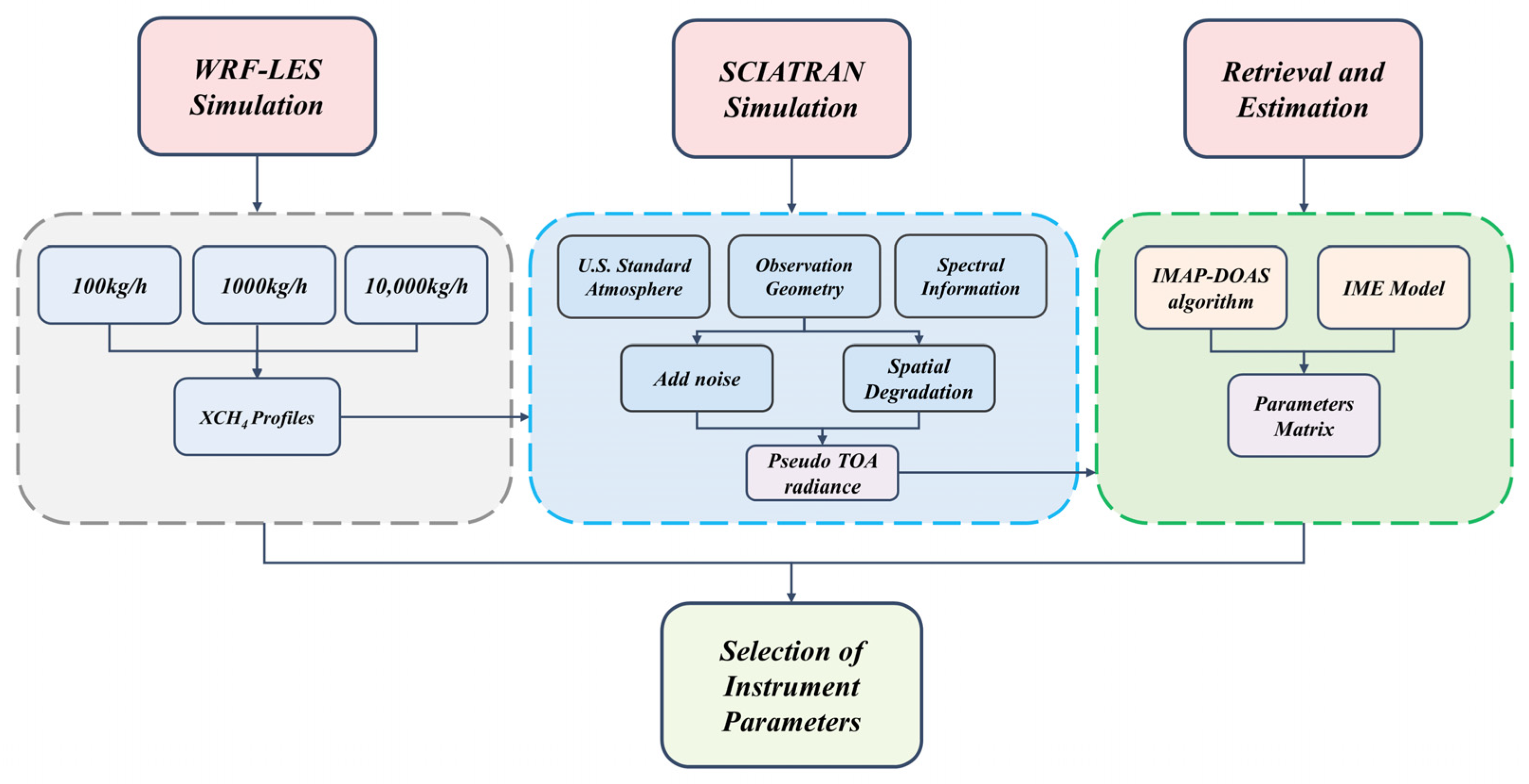
2. Materials and Methods

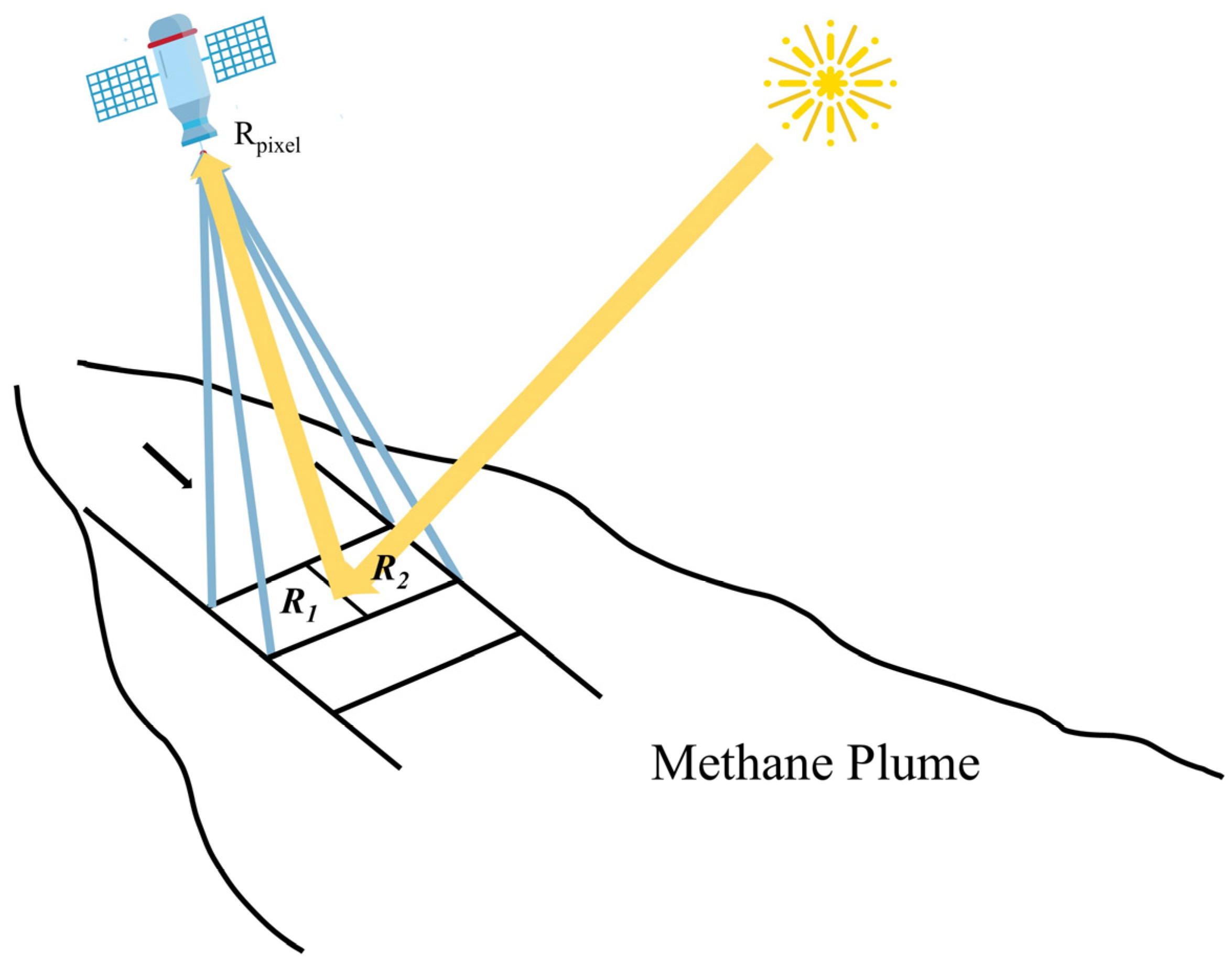
2.1. WRF-LES and Radiance Simulation

The Weather Research and Forecasting Large Eddy Simulation (WRF-LES) passive tracer was applied to generate plumes upon turbulent field dynamics [29]. Following the definition of the methane plume point source [3], the horizontal resolution of the simulation area was set to 10 m, with plume emission originating from a grid. This specific grid has the highest concentration, and is typically used as the reference for determining the location of emission sources. The simulation domain was 4 km × 4 km × 2 km along the x, y, and z axes, respectively. The model parameters, such as wind speed, mixed layer height, and temperature profile entered used in simulations were similar to those described by Varon et al. [30]. For the daytime troposphere, a mixed layer height of 1100 m and a uniform temperature of 300 K are assumed. A three-dimensional simulation of methane plumes was performed, with ΔXCH₄ obtained vertically, integrating the simulated concentration profiles. The simulation lasted for three hours, with the first two dedicated to establishing the turbulent field. The final hour was selected the for instantaneous plume analysis. Figure 2 illustrates the instantaneous plume morphology for a 10 m wind of 3 m/s and an emission rate of 1000 kg/h. Emission rates for other levels can be derived by applying a scale factor, enabling simulations for 100 kg/h and 10,000 kg/h emission rates. These specific rates allow for an evaluation of how various satellite parameters influence the detection and quantification of methane plumes of differing levels, thus assessing the sensitivity and performance of satellite-based methane monitoring systems.

Based on the simulated emission plume, the SCIATRAN radiative transfer model was employed to calculate the radiance of varying methane concentrations [31]. Absorption cross-sections were obtained from the HITRAN 2020 database, with a line-by-line absorption calculation employed to simulate radiative transfer accurately. The forward radiance simulation included all gases with absorption features within the selected spectrum to depict a realistic state of the atmosphere. Additionally, an aerosol module was incorporated to enhance the realism of the simulations. Methane profiles were derived from simulated plume data, while the profiles of other gases were based on the U.S. Standard Atmosphere. Meanwhile, a reference 30° solar zenith angle (SZA) and 0.3 surface reflectivity with clear sky were set, respectively. Pseudo-observations were subsequently generated by convolving with the spectral response function (SRF), which varies across different parameter settings.

2.2. IMAP-DOAS Retrieval

Currently, various algorithms are employed for XCH₄ retrieval, including physical retrieval and data-driven methods. Ayasse et al. (2023) compared two such methods, matched filter and IMAP-DOAS, through emission control experiments [32]. It is suggested that the estimated results based on the IMAP-DOAS retrieval algorithm have better agreement with the true emissions. The matched filter is widely used for strong emissions where the plume occupies a small portion of the image, constructing a reference spectrum by averaging the radiance within the scene [33]. Given the limited experimental domain of this study, IMAP-DOAS was employed for pixel-by-pixel retrieval. The IMAP-DOAS algorithm, similarly to the conventional DOAS method, separates high-frequency spectral information from low-frequency spectral information, with the latter parameterized using Legendre polynomials. Within the SWIR spectrum, the absorption cross-section of methane is influenced by pressure and temperature. Additionally, maximum likelihood estimation was introduced into the algorithm, and the XCH₄ was obtained through a Gaussian Newton iterative optimization [34]. The forward model, as expressed in Equation (1), fitted low-frequency spectral information using Legendre polynomials [25]:

$$F^h\left(x\right)=I_0\left(\lambda \right)\exp \left(-A{\displaystyle \sum _{n=1}^n{s}_n{\displaystyle \sum _{l=1}^l{\tau }_{n,l}}}\right)\cdot {\displaystyle \sum _{k=0}^K{a}_k{P}_k\left(\lambda \right)}$$

(1)

In the formula, $F^h\left(x\right)$ is the high spectral resolution spectrum as simulated by the forward model for a given state vector $x$, $I_0\left(\lambda \right)$ represents the solar intensity at different wavelength $\lambda$. ${\tau }_{n,l}$ denotes the optical depth of various trace gases at different vertical levels, based on profiles from the U.S. Standard Atmosphere. $A$ is the air mass factor (AMF), which is defined as the ratio between the retrieved slant column and the atmospheric vertical column. $s_n$ serves as the scale factor to the default optical depth in the retrieval. The term $P_k$ is the kth Legendre polynomial, while $a_k$ represents coefficients optimized in the retrieval. Subsequently, a Gauss–Newton iteration was applied, as depicted in Equation (2):

$$x_{i+1}=x_a+{\left(K_i^T{S}_o^{-1}{K}_i+S_a^{-1}\right)}^{-1}{K}_i^T{S}_o^{-1}\cdot \left[y-F\left(x_i\right)+K_i\left(x_i-x_a\right)\right]$$

(2)

In this iterative process, $x_a$ represents the priori state vector, including CH₄, H₂O(g), and NO₂. We set the $x_a$ to be very large, such that the retrieved parameters were almost entirely determined by the observation data. $x_{i+1}$ represents the state vector during the iteration process. The observation error matrix $S_o$ was determined by the instrumental’s SNR, while $S_a$ is the prior error covariance matrix. $y$ is the observed backscatter top-of-atmosphere (TOA) radiance, $\mathbf{F}\left(x\right)$ is the low-resolution spectrum convolved with the SRF in the forward model. ${\mathbf{K}}_{\mathbf{i}}$ represents the Jacobian matrix, and was calculated for each iteration i of the state vector. The retrieval process was performed with around 2.3 μm, where CH₄ exhibits strong absorption features. Additionally, in this algorithm, it is also necessary to subtract the background value to derive ΔXCH₄. The background concentration was determined by taking the pixels not included in the plume mask and taking a percentile [32].

2.3. Methods for Quantifying Point Source Emission Rates

To accurately quantify methane emissions, the ΔXCH₄ needs to be related to the emissions rate, Q (kg/h). Following the approach outlined by Varon [30], ΔXCH₄ masks were extracted from the background. Taking into account the diffusion characteristics of methane plumes, the Integrated Mass Enhancement (IME) model was adopted to quantify the emission rate. The emission rate $Q$ was then calculated using the following Equation (3):

$$Q={\displaystyle \frac{U_{eff}}{L}}IME={\displaystyle \frac{U_{eff}}{L}}{\displaystyle {\sum }_{j=1}^N\Delta {\Omega }_j}{P}_j$$

(3)

The effective wind speed $U_{eff}$, a parameter representing the dissipation rate of plume turbulence, was derived from the 10 m wind field. $L$ is the plume diffusion length, which describes the spatial extent over which the plume spreads. $P_j$ is the single-pixel area in the observed plume, while $\Delta {\Omega }_j$ denotes the concentration enhancement in the pixel. The plume consists of a total of $N$ pixels, where $j=1,\dots ,N$. Error propagation was addressed following the scheme outlined by He et al. [35].

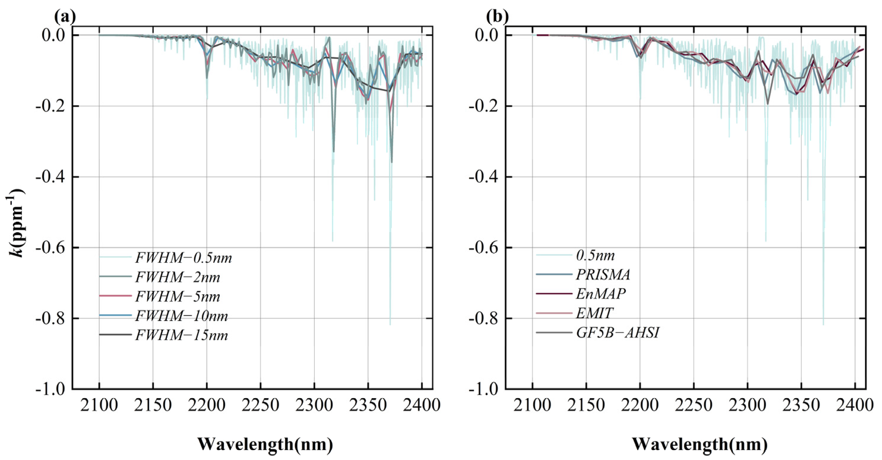
2.4. Settings for Instrument Response Functions and SNR

To explore the impact of different spectral resolutions, the full width at half maximum (FWHM) of the SRF was adjusted accordingly. Based on the spectral resolution of most hyperspectral imagers, spectral resolutions of 2 nm, 5 nm, 10 nm, and 15 nm were selected, respectively. Critical sampling was applied, with the sampling frequency set to FWHM/1.0, as implemented in the AVIRIS system [36]. In addition, the SRF was described by a Gaussian shape [12,37].

Image noise typically comprises two primary components: photon noise (PN) and constant noise (CN). PN is generally proportional to the square root of the radiance, while CN remains independent of radiance. At a given radiance level, the total noise is predominantly determined by PN, resulting in noise that scales proportionally with the square root of the radiance [21]. In this study, an idealized scenario without surface variability was simulated, eliminating the necessity to distinguish measurement noise from surface contributions.

Therefore, the noise, expressed in terms of radiance, was multiplied by a random number from a Gaussian distribution with a mean of 0 and a standard deviation of 1. This scaled noise was then added to the simulated radiance at each wavelength for each pixel. The experiment was repeated 1000 times. Noise corresponding to SNR of 100, 200, 400, 600, and 800 was added to the simulated radiance.

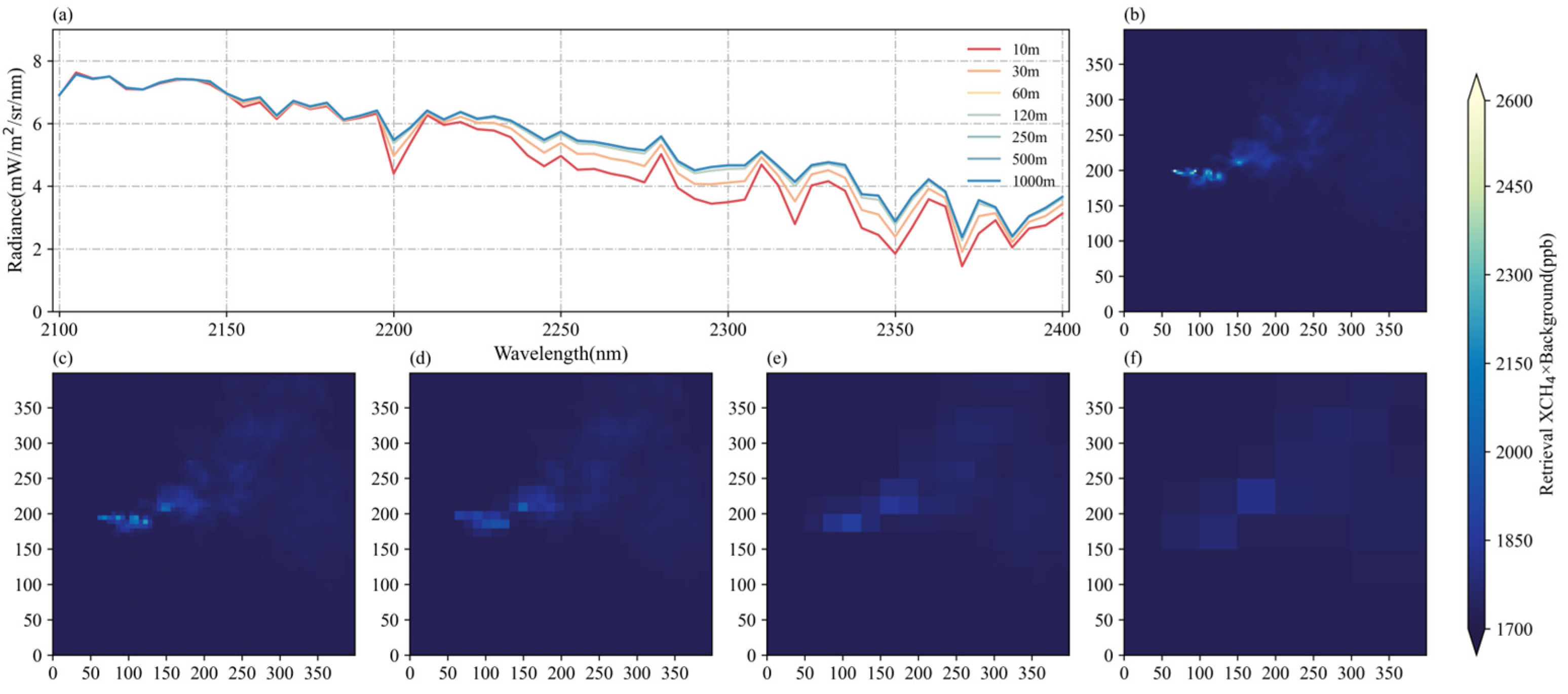
2.5. The Degradation of Spatial Resolution

To better simulate the XCH₄ of pixels detected by the satellite, it is essential to model the radiance received by instruments across varying spatial resolutions. Bhardwaj et al. (2022) modeled methane plumes with a spatial resolution of 10 m and averaged these simulations to generate 50 m satellite pseudo-observations [38]. When the spatial resolution of the satellite pixels exceeded the resolution of the plume diffusion, the radiance received was jointly influenced by the ΔXCH₄ within the mixed grids, as shown in Figure 3. The radiance observed by the satellite was the average of surrounding grids with different XCH₄. When the spatial resolution was coarsened to encompass areas with varying XCH₄, the resulting radiance could be represented as $R_{c_{pixel}}$, as illustrated in Equation (4):

$$R_{c_{pixel}}={\displaystyle \sum _{i=1}^n(\Delta S_i{R}_{c_i})/S}$$

(4)

where $R_c$ is the radiance of the sub-region, $\Delta S_i$ represents the area of the i-th small sub-region in the pixel, and $S$ represents the total area of the detection pixel. Starting with the initial 10 m of simulated plumes, we extended the spatial resolution to 30 m, 60 m, 120 m, 250 m, 500 m, and 1000 m. This range of spatial resolutions encompasses most of the current hyperspectral imagers, ensuring that the simulations are relevant to the existing satellite instruments.

3. Results

3.1. Performance of Different Spectral Resolutions

At the same spectral sampling rate, a finer spectral resolution improves the detection of methane absorption features, thereby improving the identification of subtle variations in XCH₄. The k spectrum represents the absorptive capacity of atmospheric CH₄ for radiance at specific wavelengths. As shown in Figure 4a, different spectral resolutions affect the absorption coefficient k in distinct ways. Figure 4b exhibits the methane absorption coefficient k calculated by the majority of hyperspectral imagers at varying spectral resolutions. It is evident that the instruments with coarser spectral resolution tend to blur certain spectral absorption features, leading to a smoother variation in the k spectrum. Capturing delicate methane absorption details enables the mitigation of interference from low-frequency spectral information during retrieval to a certain extent [27], which is particularly important for enhancing subsequent retrieval precision.

At the 1000 kg/h emission rate, Figure 5a–d show the retrieved ΔXCH₄ results, subtracting the background XCH₄. The finer spectral resolutions reveal a more distinct transient morphology of the plume at the same spatial resolution of 10 m and SNR of 800, with the ΔXCH₄ signal more prominently differentiated from the background. The retrieval capabilities are comparable at 2 nm and 5 nm spectral resolutions. However, an underestimation of the retrieval results is observed at coarser spectral resolutions, making regions with low ΔXCH₄ visually difficult to identify in the images. This underestimation is caused by an overall overestimation of the background and an underestimation of the plume regions. It may be attributed to the fact that as the spectral resolution decreases, it is difficult to accurately distinguish between methane absorption and other factors that influence the spectrum under the current algorithm. Also, since the retrieval was performed within a specific spectrum, limited spectral information could be one of the reasons for the poor performance obtained with coarse spectral resolution. However, this is beyond the scope of this article.

Figure 5e–h present a comparison of the simulated and the retrieved ΔXCH₄. Each plot includes linear regression lines and reference lines with a slope of 1, alongside the corresponding scatter points. Additionally, the relevant statistical variables are displayed. Meanwhile, it can be seen from the statistical variables that if the spectral resolution is 2 nm, the root mean square error (RMSE) is as low as 4.91 ppb. However, when the spectral resolution decreases to 15 nm, the RMSE increases significantly to 24.48 ppb, while the other two instrument parameters remain unchanged. Similarly, the mean absolute error (MAE) rises with coarser spectral resolutions, ranging from 3.44 ppb at 2 nm to 13.59 ppb at 15 nm. Notably, at spectral resolutions of 2 nm and 5 nm, the correlation coefficient (R²) remains comparable, indicating that the two spectral resolutions perform equally well in such little noise. These results highlight the significant impact of spectral resolution on retrieval performance.

3.2. Performance of Different Spatial Resolutions

The diffusion of a gas plume is primarily in the form of turbulence, and high spatial resolution is the key to accurately detecting their diffusion patterns. In addition, with a finer spatial resolution, the emitted gas concentration is more likely to fill the detection pixels. It could enhance the satellite’s ability to capture anomalous enhancements, resulting in a more precise depiction of plume details. The radiance received by the satellite is generally a hybrid signal from different XCH₄. It would result in attenuating fine-scale turbulent features, smearing high-concentration areas, and obscuring critical details of the plume’s complex structure. Figure 6a depicts the continuous spectral information at a 5 nm spectral resolution of the pixel where the emission is located within different spatial resolutions. With more surrounding grids included in the detection pixel, the spectrum is increasingly affected by unrelated information. Notable variations in the spectrum are represented near the absorption peak of methane as spatial resolution degraded, which in turn affects the subsequent retrieval results.

Figure 6b–f show the 1000 kg/h emission rate scene retrieval results with the background. It can be seen that the turbulent structure becomes gradually blurred as spatial resolution decreases, highlighting the impact of high resolution on capturing fine-scale details. Notably, the XCH₄ where the emission is located decreased significantly due to the influence of mixed pixels in the coarsening spatial resolution process. This decline follows a nonlinear trend; as the spatial resolution degrades from 10 m to 30 m, the XCH₄ at the detection pixel declines by 1481.44 ppb, and further decreases by 2357.00 ppb at 60 m. At the spatial resolution of 120 m, it is even difficult to determine the location of the emission pixel based on the XCH₄ distribution. Then, it suggests that high spatial resolution is effective in identifying the location of point source emissions, as mentioned in previous studies where high spatial resolution is effective in distinguishing between point source emissions from multiple distinct locations at neighboring regions [39]. When the spatial resolution is degraded to 250 m and 500 m scale, the plume’s complete morphology is no longer intact, with only a few high XCH₄ pixels discernible. Nevertheless, the influence of resolution degradation on XCH₄ diminishes slightly as emission rate levels increase. At an emission rate of 10,000 kg/h, the XCH₄ of pixels remains higher than the background field even at a spatial resolution of 500 m (See Supplementary Materials Figure S1). Conversely, for a smaller emission rate (100 kg/h), coarser spatial resolution causes the ΔXCH₄ signal to blend with the background, making it challenging to separate from the irrelevant noise. Regardless of the emission levels, the continued spatial resolution degradation would lead to a gradual disappearance of the turbulent structure and a Gaussian-resembling distribution of the plume morphology.

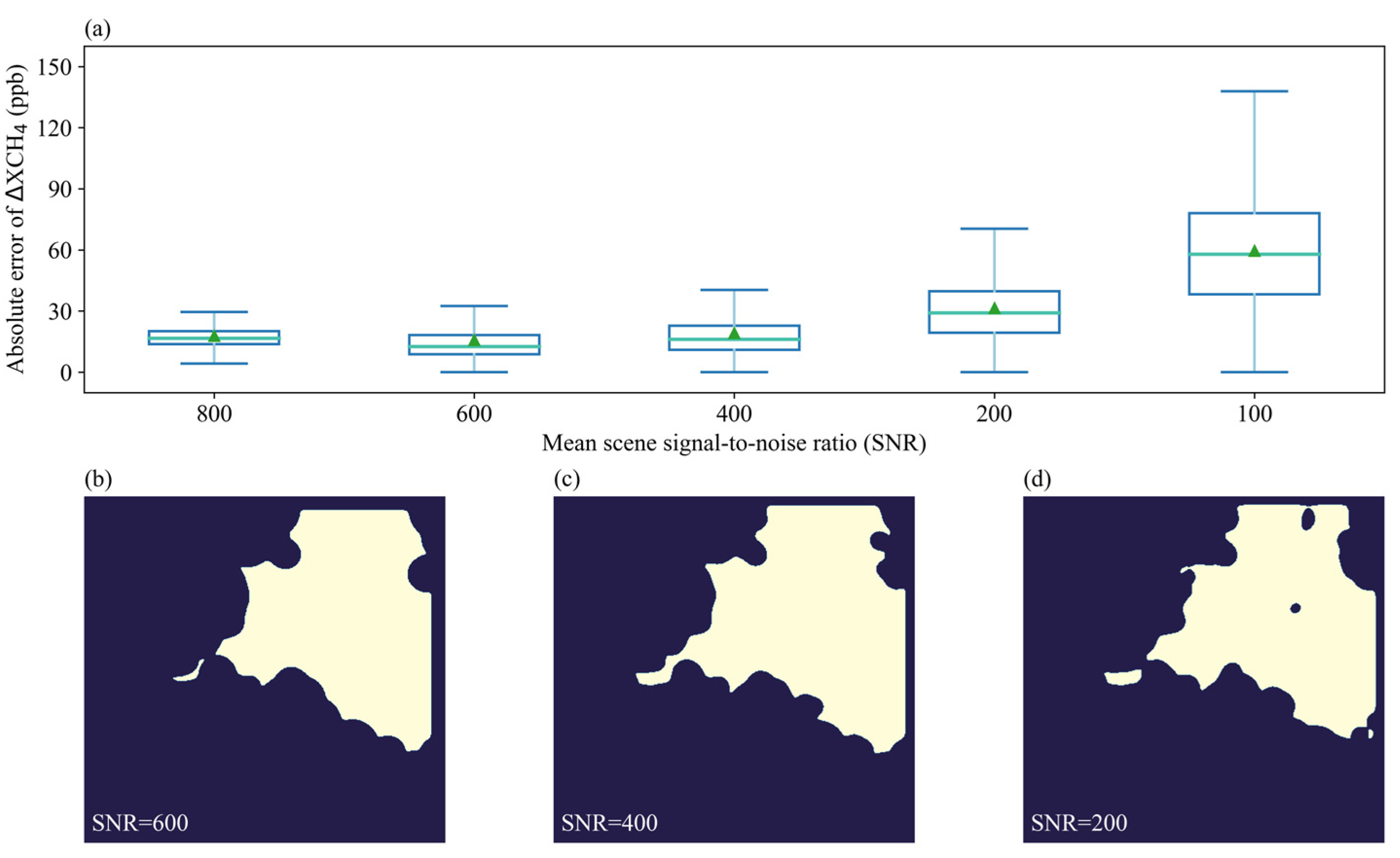
3.3. Performance of Different SNRs

SNRs are a key indicator for extracting graphical information, as excessive irrelevant signals could obscure the target signal within the noise. In addition, SNRs play a pivotal role in the retrieval process, as the $S_o$ in the IMAP-DOAS algorithm is directly tied to them. More noise leads to higher $S_o$ weighting during iterations, thereby increasing the dependence of retrieval results on the observational data. The retrieval precision of pixels gradually improves with the improvement of the SNR. The box plot of the absolute error obtained from the simulated and the retrieved ΔXCH₄, as shown in Figure 7a, indicates that the absolute error decreases as the SNR increases. The results are all based on condition with a spectral resolution of 10 nm and a spatial resolution of 10 m. At the SNR of 800, the median absolute error is 16.67 ppb, whereas at an SNR of 100, the median absolute error rises to 57.89 ppb. Meanwhile, the error distribution at high SNR, such as 800, 600, and 400, is more concentrated, suggesting higher measurement precision. In contrast, as noise increases, the error distribution becomes more discrete, with a remarkable increase in outliers, suggesting more measurement error.

Additionally, for individual plume estimation, noise is associated with the masking process that separates the plume from the background field (SNR = 600, 400, 200), as illustrated in Figure 7b–d. At a high SNR (such as 600 and 400), the plume mask boundary remains comparatively complete. However, the detected plume regions artificially shrink, and the details of the plume boundary become increasingly blurred when the SNR decreases to 200. In theory, when noise approaches the magnitude of the signal, it may result in potentially obscuring plume boundaries and make it challenging to distinguish the plume from the surrounding noise. Therefore, increasing noise enhances the likelihood of misclassifying low-concentration plume boundaries as background noise. Furthermore, if noise-induced artifacts appear within the plume, they are difficult to eliminate through mask extraction, introducing errors in subsequent quantitative analyses.

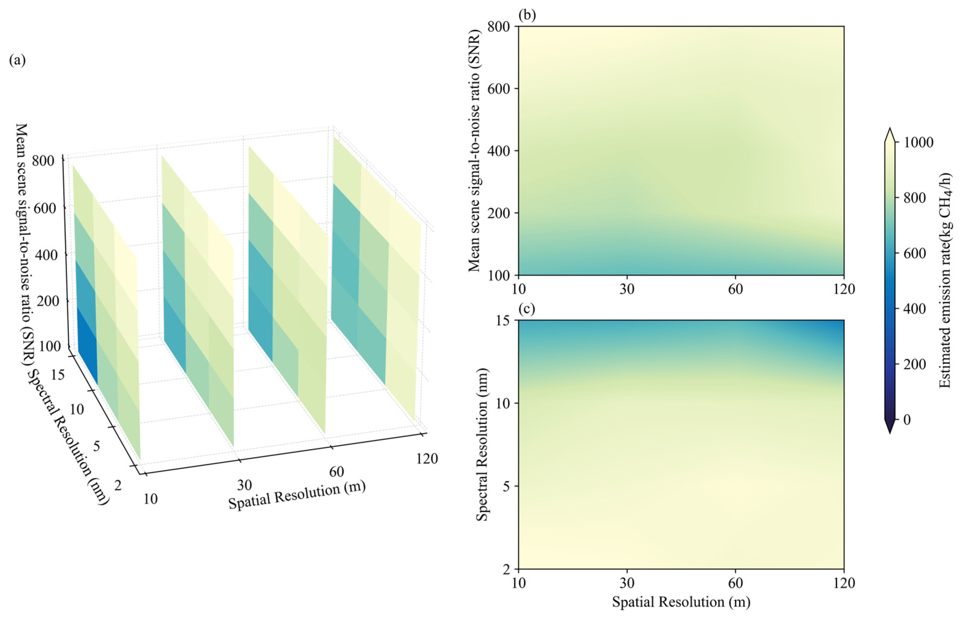
3.4. The Coupled Effect of Key Parameters on Methane Plume Retrieval

This section will discuss the coupled effect of the three instrument parameters, as reflected in the estimated emission rates. Note that directly using the emission rates estimated results for parameter comparison may introduce errors from other factors, such as errors in $U_{eff}$ and the estimation of the plume length. However, we contend that the overall trend in the estimated emission results could effectively indicate variations in the sensitivity of the instrument parameters. Due to the limitations of the simulation domain and the plume segmentation process, we restrict the spatial resolution from 10 m to 120 m. The total estimated results for three different emission levels are shown in Figure 8. It shows the estimation results clustered by different spatial resolutions (10 m, 30 m, 60 m, and 120 m). It can be seen that variations in instrument parameters lead to a certain degree of underestimation in the estimated emission rates, but such underestimations extend as methane emissions rate decrease. The estimated error for an emission rate of 10,000 kg/h is almost below 50%. As the emission rate decreases to 100 kg/h, the overall estimated error gradually increases, with the error even reaching up to 100%. A possible explanation is that higher emission rates lead to stronger ΔXCH₄ signals, resulting in a sharper contrast with the background. Consequently, a more complete plume was detected. With an emission of 100 kg/h at the spatial resolution of 10 m, the most striking ΔXCH₄ of the plume region remains below 100 ppb, and the weak concentration signal is easily submerged in the noise. In addition, changes in spatial resolution have the most marked impact on small emission rate plumes, and the underestimation gradually increases as spatial resolution degrades. Meanwhile, the estimated results also exhibit some changes with the other two instrument parameters.

Since the estimated results of different emissions levels show similar trends across various instrument parameters, a detailed analysis was conducted at 1000 kg/h, as shown in Figure 9. Results for other emission rates are provided in the Supplementary Materials. As shown in the three-dimensional distribution plot of Figure 9a, degrading the spatial resolution from 10 m to 120 m has regular estimated results. Within this range of spatial degradation, ΔXCH₄ remains easily distinguished from the background. At a high retrieval precision of a single pixel, characterized by a finer spectral resolution (2 nm or 5 nm) and higher SNR (from 400 to 800), plume emission rates were estimated more accurately, with less than 20% estimated error at all spatial resolutions. However, at a moderate spectral resolution (10 nm or 15 nm), the quantification results are underestimated generally. As mentioned in Section 3.1, the error in the single-pixel XCH₄ rises with coarser spectral resolution. Especially in low SNR scenarios, the plume signal is often overwhelmed by the noise, resulting in a greater degree of underestimation. For the estimation results of small emission rates (100 kg/h), see the Supplementary Materials Figure S2. When the spatial resolution was coarsened to 120 m, both the spectral resolution and SNR were suboptimal, making it difficult to be effectively quantified under the current retrieval algorithm method. This indicates that spatial resolution is a critical prerequisite for detecting small emission plumes; whereas, for plumes with much higher emission rates, although the ΔXCH₄ decreases with the change in spatial resolution, it remains greater than the background, and minor variations in spatial resolution (from 10 m to 120 m) have a negligible impact on plume quantification.

In addition, it can be seen from the figure that changes in spectral resolution and SNR would also have a marked impact on the estimated results. The correlation of the two parameters is not linear, but rather follows a concave distribution, suggesting that increasing the spectral resolution can quantify the plume more precisely than enhancing SNR, in agreement with the verification of the retrieval precision by Cusworth [25]. This is due to the fact that increasing the spectral resolution can effectively enhance the number of spectral samples in the retrieval spectrum, which in turn makes the methane absorption features more pronounced and improves the spectral contrast relative to the continuous spectrum. The limitations of spectral resolution and SNR can be mitigated by applying advanced algorithms. Methods such as matched filter could maximize the SNR, while TOA reflectance can be utilized to achieve effective retrievals, even at a coarse spectral resolution. Figure 9b illustrates the relationship between spatial resolution and SNR at the specific spectral resolution of 2 nm. Regardless of changes in spatial resolution, the low SNR notably impacted the estimated results. When the SNR was lower than 200, the estimated errors were generally more than 30%. In addition, there was little improvement in estimation when the SNR increased from 400 to 800, indicating similar performance at these high SNRs. Figure 9c presents the results when slicing the matrix at the fixed SNR of 800. It shows that underestimation was consistently exhibited at the coarser spectral resolutions, irrespective of the spatial resolution. This finding emphasizes the importance of achieving high spectral resolutions.

4. Discussion

As the range of simulated instrument parameters does not fully cover all satellites, interpolation was applied to the estimated matrix to address these gaps. The pseudo-observation radiance spectrum was generated using the current on-orbit satellite instrument parameters, which are listed in

Table 1. Retrieved emission rate (kg/h) based on different parameters of hyperspectral imagers.

Satellite	Spatial Resolution	Spectral Resolution (Average FWHM)	SNR	Predicted Emission Rate (kg/h)	Retrieved Emission Rate (kg/h)	Type of Spectrometer	Reference
PRISMA	30	~10	200	639.37	644.92 ± 365.99	Dispersive (prism)	[11]
EnMAP	30	~7.8	230	707.43	710.60 ± 403.24	Dispersive (prism)	[12]
EMIT	60	~8.4	750	894.73	899.94 ± 510.92	Dispersive (grating)	[23]
GF5B-AHSI	30	8.25	200	684.70	670.69 ± 380.60	Dispersive (grating)	[41]

. The same was ensured in reflectivity and SZA across all simulations. The analysis focused on the currently leading hyperspectral imagers: PRISMA, EnMAP, EMIT, and GF5B-AHSI. These different hyperspectral imagers respond differently to the methane absorption spectrum, as shown in Figure 4b. Taking the plume of 1000 kg/h as an example, by comparing the interpolation results with the pseudo-observation retrieval results, the two types of data have a certain consistency. This suggests that the parameter matrix we established is representative of the selection of instrument parameters. However, the estimated results of the true satellite instrument parameters are still slightly different from the interpolation results. This discrepancy may be attributed to the spectral sampling in the SRF, which is one in our experiment, but varies across the selected hyperspectral imagers. In addition, this difference could also come from the error caused by the interpolation. Moreover, existing satellites underestimate the emission rate to a certain extent. It is possible that under the current algorithms, the limited spectral resolution hinders the ability to separate the methane absorption features from the mixed signals, and the estimation process by the plume model also introduces errors. A similar underestimation was found in EMIT in estimating the CO₂ plume emission rate [40].

We present a range of satellite instrument parameter options for methane plume monitoring, but do not incorporate instruments with finer spectral resolution (such as GHGSats, MethaneSat, etc.) Additionally, from the perspective of noise sources, only instrument noise is considered, and the impact of surface type is not included. All of these will be addressed in our future work. However, our conclusions still have some guidance for the current detection needs of methane plumes. Scientific instrument parameters are important prerequisites for achieving high-precision plume detection. Regarding instrument design, the spatial resolution can be improved by increasing the aperture of the optical system or optimizing the instrument’s orbit. This is consistent with our experimental hypothesis that the instrument aperture can obtain sufficient radiance intensity regardless of the parameters. In addition, the optical system, detector parameters, and exposure time of the instrument collectively impact the SNR of the instrument. Since the estimation accuracy is more effectively improved by spectral resolution than SNR, the design of the instrument could focus on improving the spectral resolution. Optimizing the design of the optical system is crucial to the spectral resolution. Both dispersion spectroscopy and interference imaging spectrometers can achieve good spectroscopic effects. The dispersive spectroscopic systems can be further divided into prism and grating type. Prism spectrometers, used in missions such as PRISMA and EnMAP [12,42], are widely adopted and straightforward techniques for spectral imaging. In such systems, the spectral resolution is inversely proportional to the width of the incident slit. It would reduce detection sensitivity and has a negative impact on the SNR in pursuit of high spectral resolution. The grating spectrometers used by EMIT and GF5B-AHSI have more complex optical systems [43,44]. On the other hand, the interferometric imaging spectrometers, represented by Fourier transform spectrometers, offer intrinsic advantages. Their high spectral resolution and efficient energy utilization makes them well-suited for applications demanding fine spectral detail. From a performance perspective, dispersive spectrometers provide high spectral resolution and accuracy while maintaining a relatively simple and compact design, especially the prism spectrometers. In contrast, interferometric spectrometers generally face challenges for data transmission and processing. In addition, due to their more complex optical design and larger volume, interferometric spectrometers are typically better suited for large satellite missions. However, the Fabry–Pérot interferometer stands as an exception to this, which could achieve fine spectral resolution detection in a compact volume; however, it is limited to specific spectral bands [45]. Considering launch costs and the limitations of payload mass and volume, dispersive spectrometers are well-suited for most methane plume requirements, as shown in Table 1. For achieving finer spectral resolution, the Fabry–Pérot interferometer is an alternative, as well.

5. Conclusions

To investigate the impact of spatial resolution, spectral resolution, and SNR on methane plume estimation accuracy. We simulated methane plumes with different emission rates and generated TOA radiance datasets. Sensitivity analysis was conducted on the instrument parameters using the IMAP-DOAS retrieval algorithm and the IME model. To evaluate the effects of varying spatial resolutions, we also simulated radiance within hybrid pixels.

Regarding the impact of individual parameters, fine spectral resolution and high SNR are the keys to accurately retrieve single-pixel XCH₄. Meanwhile, the spatial resolution is an important prerequisite for identifying emission point locations as well as small plume emission. In addition, according to the quantification results of the three instrument parameters, the estimated error has a certain relationship with the emission rates. Specifically, for plumes with large emission rates (10,000 kg/h), the estimated error is generally below 50% within the parameter range of most current hyperspectral imagers. In contrast, for plumes with an emission rate of approximately 100 kg/h, the estimated error can reach around 100%.

Based on the three-dimensional estimation matrix built from instrument parameters, we found that although spatial resolution degradation decreases XCH₄ in the pixel, larger emission rates (1000 kg/h or 10,000 kg/h) remain distinguishable from the background, and quantifiable even at 120 m resolution. Notably, finer spatial resolution captures plume details and improves small-emission plume (100 kg/h) detection capabilities. Since small emission rates account for the majority of plumes, achieving high spatial resolution observations should be an important priority for future satellite missions. In addition, regardless of the spatial scale, finer spectral resolution (2 nm or 5 nm) is vital for accurately estimating methane plumes, as it enhances single-pixel retrieval precision. Therefore, designing instruments to achieve fine spectral resolution is a key consideration. The dispersive spectrometers or Fabry–Pérot interferometers are well-suited to meet current detection needs. Moreover, increasing the SNR from 400 to 800 does not significantly improve the overall quantification accuracy.

To verify the feasibility of the established matrix, we interpolated it to span the parameter range of existing satellite instruments. In addition, pseudo-observations convolved with the current satellite response function were generated for comparison. Due to the slight difference in spectral sampling rate, the estimation results are slightly different. Nevertheless, these results sufficiently demonstrate that the constraint relationships between the simulated instrument parameters are representative. In total, enhancing the spectral resolution can markedly improve the quantification performance. Increasing spatial resolution can significantly increase the accuracy of small emission plume estimation, provided that high spectral resolution is maintained. A scientific SNR helps reduce estimation errors, but there is no need to pursue an extremely high SNR. Our future research will consider a wider spectral range and more satellite instruments, as well as various surface types.

References

1. Naik, V.; Szopa, S.; Adhikary, B.; Artaxo, P.; Berntsen, T.; Collins, W.D.; Fuzzi, S.; Gallardo, L.; Kiendler Scharr, A.; Klimont, Z.; et al. Short-Lived Climate Forcers. In Climate Change 2021: The Physical Science Basis. Contribution of Working Group I to the Sixth Assessment Report of the Intergovernmental Panel on Climate Change; Masson-Delmotte, V., Zhai, P., Pirani, A., Connors, S.L., Peán, C., Berger, S., Caud, N., Chen, Y., Goldfarb, L., Gomis, M.L., Eds.; Cambridge University Press: Cambridge, UK, 2021; pp. 817–921. [Google Scholar]
2. Saunois, M.; Stavert, A.R.; Poulter, B.; Bousquet, P.; Canadell, J.G.; Jackson, R.B.; Raymond, P.A.; Dlugokencky, E.J.; Houweling, S.; Patra, P.K.; et al. The Global Methane Budget 2000–2017. Earth Syst. Sci. Data 2020, 12, 1561–1623. [Google Scholar] [CrossRef]
3. Duren, R.M.; Thorpe, A.K.; Foster, K.T.; Rafiq, T.; Hopkins, F.M.; Yadav, V.; Bue, B.D.; Thompson, D.R.; Conley, S.; Colombi, N.K.; et al. California’s Methane Super-Emitters. Nature 2019, 575, 180–184. [Google Scholar] [CrossRef]
4. Brandt, A.R.; Heath, G.A.; Cooley, D. Methane Leaks from Natural Gas Systems Follow Extreme Distributions. Environ. Sci. Technol. 2016, 50, 12512–12520. [Google Scholar] [CrossRef]
5. Erland, B.M.; Thorpe, A.K.; Gamon, J.A. Recent Advances Toward Transparent Methane Emissions Monitoring: A Review. Environ. Sci. Technol. 2022, 56, 16567–16581. [Google Scholar] [CrossRef] [PubMed]
6. Jacob, D.J.; Varon, D.J.; Cusworth, D.H.; Dennison, P.E.; Frankenberg, C.; Gautam, R.; Guanter, L.; Kelley, J.; McKeever, J.; Ott, L.E.; et al. Quantifying Methane Emissions from the Global Scale down to Point Sources Using Satellite Observations of Atmospheric Methane. Atmos. Chem. Phys. 2022, 22, 9617–9646. [Google Scholar] [CrossRef]
7. Yoshida, Y.; Ota, Y.; Eguchi, N.; Kikuchi, N.; Nobuta, K.; Tran, H.; Morino, I.; Yokota, T. Retrieval Algorithm for CO2 and CH4 Column Abundances from Short-Wavelength Infrared Spectral Observations by the Greenhouse Gases Observing Satellite. Atmos. Meas. Tech. 2011, 4, 717–734. [Google Scholar] [CrossRef]
8. Schepers, D.; Guerlet, S.; Butz, A.; Landgraf, J.; Frankenberg, C.; Hasekamp, O.; Blavier, J.-F.; Deutscher, N.M.; Griffith, D.W.T.; Hase, F.; et al. Methane Retrievals from Greenhouse Gases Observing Satellite (GOSAT) Shortwave Infrared Measurements: Performance Comparison of Proxy and Physics Retrieval Algorithms. J. Geophys. Res. Atmos. 2012, 117. [Google Scholar] [CrossRef]
9. Hu, H.; Hasekamp, O.; Butz, A.; Galli, A.; Landgraf, J.; Aan de Brugh, J.; Borsdorff, T.; Scheepmaker, R.; Aben, I. The Operational Methane Retrieval Algorithm for TROPOMI. Atmos. Meas. Tech. 2016, 9, 5423–5440. [Google Scholar] [CrossRef]
10. Qu, Z.; Jacob, D.J.; Shen, L.; Lu, X.; Zhang, Y.; Scarpelli, T.R.; Nesser, H.; Sulprizio, M.P.; Maasakkers, J.D.; Bloom, A.A.; et al. Global Distribution of Methane Emissions: A Comparative Inverse Analysis of Observations from the TROPOMI and GOSAT Satellite Instruments. Atmos. Chem. Phys. 2021, 21, 14159–14175. [Google Scholar] [CrossRef]
11. Guanter, L.; Irakulis-Loitxate, I.; Gorroño, J.; Sánchez-García, E.; Cusworth, D.H.; Varon, D.J.; Cogliati, S.; Colombo, R. Mapping Methane Point Emissions with the PRISMA Spaceborne Imaging Spectrometer. Remote Sens. Environ. 2021, 265, 112671. [Google Scholar] [CrossRef]
12. Storch, T.; Honold, H.-P.; Chabrillat, S.; Habermeyer, M.; Tucker, P.; Brell, M.; Ohndorf, A.; Wirth, K.; Betz, M.; Kuchler, M.; et al. The EnMAP Imaging Spectroscopy Mission towards Operations. Remote Sens. Environ. 2023, 294, 113632. [Google Scholar] [CrossRef]
13. Siddiqui, A.; Halder, S.; Kannemadugu, H.B.S.; Prakriti; Chauhan, P. Detecting Methane Emissions from Space in India: Analysis Using EMIT and Sentinel-5P TROPOMI Datasets. J. Indian Soc. Remote Sens. 2024, 52, 1901–1921. [Google Scholar] [CrossRef]
14. He, Z.; Gao, L.; Liang, M.; Zeng, Z.-C. A Survey of Methane Point Source Emissions from Coal Mines in Shanxi Province of China Using AHSI on Board Gaofen-5B. Atmos. Meas. Tech. 2024, 17, 2937–2956. [Google Scholar] [CrossRef]
15. Jervis, D.; McKeever, J.; Durak, B.O.A.; Sloan, J.J.; Gains, D.; Varon, D.J.; Ramier, A.; Strupler, M.; Tarrant, E. The GHGSat-D Imaging Spectrometer. Atmos. Meas. Tech. 2021, 14, 2127–2140. [Google Scholar] [CrossRef]
16. Chan Miller, C.; Roche, S.; Wilzewski, J.S.; Liu, X.; Chance, K.; Souri, A.H.; Conway, E.; Luo, B.; Samra, J.; Hawthorne, J.; et al. Methane Retrieval from MethaneAIR Using the CO2 Proxy Approach: A Demonstration for the Upcoming MethaneSAT Mission. Atmos. Meas. Tech. 2024, 17, 5429–5454. [Google Scholar] [CrossRef]
17. Irakulis-Loitxate, I.; Guanter, L.; Liu, Y.-N.; Varon, D.J.; Maasakkers, J.D.; Zhang, Y.; Chulakadabba, A.; Wofsy, S.C.; Thorpe, A.K.; Duren, R.M.; et al. Satellite-Based Survey of Extreme Methane Emissions in the Permian Basin. Sci. Adv. 2021, 7, eabf4507. [Google Scholar] [CrossRef]
18. Irakulis-Loitxate, I.; Guanter, L.; Maasakkers, J.D.; Zavala-Araiza, D.; Aben, I. Satellites Detect Abatable Super-Emissions in One of the World’s Largest Methane Hotspot Regions. Environ. Sci. Technol. 2022, 56, 2143–2152. [Google Scholar] [CrossRef] [PubMed]
19. Sherwin, E.D.; Rutherford, J.S.; Chen, Y.; Aminfard, S.; Kort, E.A.; Jackson, R.B.; Brandt, A.R. Single-Blind Validation of Space-Based Point-Source Detection and Quantification of Onshore Methane Emissions. Sci. Rep. 2023, 13, 3836. [Google Scholar] [CrossRef]
20. MacLean, J.-P.W.; Girard, M.; Jervis, D.; Marshall, D.; McKeever, J.; Ramier, A.; Strupler, M.; Tarrant, E.; Young, D. Offshore Methane Detection and Quantification from Space Using Sun Glint Measurements with the GHGSat Constellation. Atmos. Meas. Tech. 2024, 17, 863–874. [Google Scholar] [CrossRef]
21. Roger, J.; Irakulis-Loitxate, I.; Valverde, A.; Gorroño, J.; Chabrillat, S.; Brell, M.; Guanter, L. High-Resolution Methane Mapping with the EnMAP Satellite Imaging Spectroscopy Mission. IEEE Trans. Geosci. Remote Sens. 2023, 62, 1–12. [Google Scholar] [CrossRef]
22. Han, G.; Pei, Z.; Shi, T.; Mao, H.; Li, S.; Mao, F.; Ma, X.; Zhang, X.; Gong, W. Unveiling Unprecedented Methane Hotspots in China’s Leading Coal Production Hub: A Satellite Mapping Revelation. Geophys. Res. Lett. 2024, 51, e2024GL109065. [Google Scholar] [CrossRef]
23. Thorpe, A.K.; Green, R.O.; Thompson, D.R.; Brodrick, P.G.; Chapman, J.W.; Elder, C.D.; Irakulis-Loitxate, I.; Cusworth, D.H.; Ayasse, A.K.; Duren, R.M.; et al. Attribution of Individual Methane and Carbon Dioxide Emission Sources Using EMIT Observations from Space. Sci. Adv. 2023, 9, eadh2391. [Google Scholar] [CrossRef]
24. Kruse, F. The Effects of Spatial Resolution, Spectral Resolution, and SNR on Geologic. In Proceedings of the 9th JPL Airborne Earth Science Workshop, Monterey, CA, USA, 27 February–2 March 2001. [Google Scholar]
25. Cusworth, D.H.; Jacob, D.J.; Varon, D.J.; Chan Miller, C.; Liu, X.; Chance, K.; Thorpe, A.K.; Duren, R.M.; Miller, C.E.; Thompson, D.R.; et al. Potential of Next-Generation Imaging Spectrometers to Detect and Quantify Methane Point Sources from Space. Atmos. Meas. Tech. 2019, 12, 5655–5668. [Google Scholar] [CrossRef]
26. Ayasse, A.K.; Dennison, P.E.; Foote, M.; Thorpe, A.K.; Joshi, S.; Green, R.O.; Duren, R.M.; Thompson, D.R.; Roberts, D.A. Methane Mapping with Future Satellite Imaging Spectrometers. Remote Sens. 2019, 11, 3054. [Google Scholar] [CrossRef]
27. Jongaramrungruang, S.; Matheou, G.; Thorpe, A.K.; Zeng, Z.-C.; Frankenberg, C. Remote Sensing of Methane Plumes: Instrument Tradeoff Analysis for Detecting and Quantifying Local Sources at Global Scale. Atmos. Meas. Tech. 2021, 14, 7999–8017. [Google Scholar] [CrossRef]
28. Scafutto, R.D.M.; Van Der Werff, H.; Bakker, W.H.; Van Der Meer, F.; Souza Filho, C.R.D. An Evaluation of Airborne SWIR Imaging Spectrometers for CH4 Mapping: Implications of Band Positioning, Spectral Sampling and Noise. Int. J. Appl. Earth Obs. Geoinf. 2021, 94, 102233. [Google Scholar] [CrossRef]
29. Bhimireddy, S.R.; Bhaganagar, K. Implementing a New Formulation in WRF-LES for Buoyant Plume Simulations: bPlume-WRF-LES Model. Mon. Weather Rev. 2021, 149, 2299–2319. [Google Scholar] [CrossRef]
30. Varon, D.J.; Jacob, D.J.; McKeever, J.; Jervis, D.; Durak, B.O.A.; Xia, Y.; Huang, Y. Quantifying Methane Point Sources from Fine-Scale Satellite Observations of Atmospheric Methane Plumes. Atmos. Meas. Tech. 2018, 11, 5673–5686. [Google Scholar] [CrossRef]
31. Mei, L.; Rozanov, V.; Rozanov, A.; Burrows, J.P. SCIATRAN Software Package (V4.6): Update and Further Development of Aerosol, Clouds, Surface Reflectance Databases and Models. Geosci. Model Dev. 2023, 16, 1511–1536. [Google Scholar] [CrossRef]
32. Ayasse, A.K.; Cusworth, D.; O’Neill, K.; Fisk, J.; Thorpe, A.K.; Duren, R. Performance and Sensitivity of Column-Wise and Pixel-Wise Methane Retrievals for Imaging Spectrometers. Atmos. Meas. Tech. 2023, 16, 6065–6074. [Google Scholar] [CrossRef]
33. Huang, Y.; Natraj, V.; Zeng, Z.-C.; Kopparla, P.; Yung, Y.L. Quantifying the Impact of Aerosol Scattering on the Retrieval of Methane from Airborne Remote Sensing Measurements. Atmos. Meas. Tech. 2020, 13, 6755–6769. [Google Scholar] [CrossRef]
34. Frankenberg, C.; Platt, U.; Wagner, T. Iterative Maximum a Posteriori (IMAP)-DOAS for Retrieval of Strongly Absorbing Trace Gases: Model Studies for CH4 and CO2 Retrieval from near Infrared Spectra of SCIAMACHY Onboard. Atmos. Chem. Phys. 2005, 5, 9–22. [Google Scholar] [CrossRef]
35. He, T.-L.; Boyd, R.J.; Varon, D.J.; Turner, A.J. Increased Methane Emissions from Oil and Gas Following the Soviet Union’s Collapse. Proc. Natl. Acad. Sci. USA 2024, 121, e2314600121. [Google Scholar] [CrossRef]
36. Thorpe, A.K.; Frankenberg, C.; Roberts, D.A. Retrieval Techniques for Airborne Imaging of Methane Concentrations Using High Spatial and Moderate Spectral Resolution: Application to AVIRIS. Atmos. Meas. Tech. 2014, 7, 491–506. [Google Scholar] [CrossRef]
37. Acito, N.; Diani, M.; Corsini, G. PRISMA Spatial Resolution Enhancement by Fusion with Sentinel-2 Data. IEEE J. Sel. Top. Appl. Earth Obs. Remote Sens. 2022, 15, 62–79. [Google Scholar] [CrossRef]
38. Bhardwaj, P.; Kumar, R.; Mitchell, D.A.; Randles, C.A.; Downey, N.; Blewitt, D.; Kosovic, B. Evaluating the Detectability of Methane Point Sources from Satellite Observing Systems Using Microscale Modeling. Sci. Rep. 2022, 12, 17425. [Google Scholar] [CrossRef] [PubMed]
39. Sánchez-García, E.; Gorroño, J.; Irakulis-Loitxate, I.; Varon, D.J.; Guanter, L. Mapping Methane Plumes at Very High Spatial Resolution with the WorldView-3 Satellite. Atmos. Meas. Tech. 2022, 15, 1657–1674. [Google Scholar] [CrossRef]
40. Nelson, R.R.; Cusworth, D.H.; Thorpe, A.K.; Kim, J.; Elder, C.D.; Nassar, R.; Mastrogiacomo, J.-P. Comparing Point Source CO2 Emission Rate Estimates from Near-Simultaneous OCO-3 and EMIT Observations. Geophys. Res. Lett. 2024, 51, e2024GL113002. [Google Scholar] [CrossRef]
41. Ye, B.; Tian, S.; Cheng, Q.; Ge, Y. Application of Lithological Mapping Based on Advanced Hyperspectral Imager (AHSI) Imagery Onboard Gaofen-5 (GF-5) Satellite. Remote Sens. 2020, 12, 3990. [Google Scholar] [CrossRef]
42. Cogliati, S.; Sarti, F.; Chiarantini, L.; Cosi, M.; Lorusso, R.; Lopinto, E.; Miglietta, F.; Genesio, L.; Guanter, L.; Damm, A.; et al. The PRISMA Imaging Spectroscopy Mission: Overview and First Performance Analysis. Remote Sens. Environ. 2021, 262, 112499. [Google Scholar] [CrossRef]
43. Liu, Y.-N.; Zhang, J.; Zhang, Y.; Sun, W.-W.; Jiao, L.-L.; Sun, D.-X.; Hu, X.-N.; Ye, X.; Li, Y.-D.; Liu, S.-F.; et al. The Advanced Hyperspectral Imager: Aboard China’s GaoFen-5 Satellite. IEEE Geosci. Remote Sens. Mag. 2019, 7, 23–32. [Google Scholar] [CrossRef]
44. Thompson, D.R.; Green, R.O.; Bradley, C.; Brodrick, P.G.; Mahowald, N.; Dor, E.B.; Bennett, M.; Bernas, M.; Carmon, N.; Chadwick, K.D.; et al. On-Orbit Calibration and Performance of the EMIT Imaging Spectrometer. Remote Sens. Environ. 2024, 303, 113986. [Google Scholar] [CrossRef]
45. Vargas-Rodríguez, E.; Rutt, H.N. Design of CO, CO2 and CH4 Gas Sensors Based on Correlation Spectroscopy Using a Fabry–Perot Interferometer. Sens. Actuators B Chem. 2009, 137, 410–419. [Google Scholar] [CrossRef]
Figure 1. A schematic of the study.
Remotesensing 17 00634 g001
Figure 2. Instantaneous ΔXCH4 plume image for 10 m spatial resolution with an emission rate of 1000 kg/h, simulated by WRF-LES.
Remotesensing 17 00634 g002
Figure 3. Schematic representation of satellite radiance received at different spatial resolutions.
Remotesensing 17 00634 g003
Figure 4. (a) k spectrum convolved with different spectral resolution; (b) same as (a), but convolved with different satellite sensors.
Remotesensing 17 00634 g004
Figure 5. With the emission rate of 1000 kg/h, (ad) retrieved ΔXCH4 images with different spectral resolutions (2 nm, 5 nm, 10 nm, 15 nm, respectively); (eh) scatterplots comparing simulated and retrieved ΔXCH4 with different spectral resolutions (2 nm, 5 nm, 10 nm, 15 nm, respectively). The solid line is the linear regression of these scattered points. The dashed line is the line with a slope of 1.
Remotesensing 17 00634 g005
Figure 6. With the emission rate of 1000 kg/h, (a) simulated TOA radiance at different spatial resolutions; (bf) scenes retrieval at spatial resolutions of 30 m, 60 m, 120 m, 250 m, 500 m. All simulations were conducted with a spectral resolution of 5 nm and SNR of 600.
Remotesensing 17 00634 g006
Figure 7. With the emission rate of 1000 kg/h, (a) the ΔXCH4 absolute error box plot of simulated and retrieved ΔXCH4 at the spatial resolution of 10 m and spectral resolution of 10 nm, with SNRs of 800, 600, 400, and 200, 100, respectively; (bd) plume masks under varying SNRs of 800, 600, 400, 200, and 100.
Remotesensing 17 00634 g007
Figure 8. Estimated results of plumes with varying emission rates under different instrument parameters: (a) 10,000 kg/h; (b) 1000 kg/h; (c) 100 kg/h.
Remotesensing 17 00634 g008
Figure 9. (a) Estimated emissions of retrieval with different key parameters for 1000 kg/h simulated emissions; (b) the relationship between spatial resolution and SNR at 2 nm spectral resolution; (c) the relationship between spatial resolution and spectral resolution at SNR of 800.
Remotesensing 17 00634 g009