Anomaly-Aware Tropical Cyclone Track Prediction Using Multi-Scale Generative Adversarial Networks

Abstract

Tropical cyclones (TCs) frequently encompass multiple hazards, including extreme winds, intense rainfall, storm surges, flooding, lightning, and tornadoes. Accurate methods for forecasting TC tracks are essential to mitigate the loss of life and property associated with these hazards. Despite significant advancements, accurately forecasting the paths of TCs remains a challenge, particularly when they interact with complex land features, weaken into remnants after landfall, or are influenced by abnormal satellite observations. To address these challenges, we propose a generative adversarial network (GAN) model with a multi-scale architecture that processes input data at four distinct resolution levels. The model is designed to handle diverse inputs, including satellite cloud imagery, vorticity, wind speed, and geopotential height, and it features an advanced center detection algorithm to ensure precise TC center identification. Our model demonstrates robustness during testing, accurately predicting TC paths over both ocean and land while also identifying weak TC remnants. Compared to other deep learning approaches, our method achieves superior detection accuracy with an average error of 41.0 km for all landfalling TCs in Australia from 2015 to 2020. Notably, for five TCs with abnormal satellite observations, our model maintains high accuracy with a prediction error of 35.2 km, which is a scenario often overlooked by other approaches.

1. Introduction

Tropical cyclones (TCs) rank among the most destructive and costly natural disasters affecting coastal regions [1]. Their devastating impact primarily arises from two factors: powerful destructive wind and severe flooding caused by intense rainfall, both of which are concentrated around the TC center. So, the accurate and timely forecasting of TC centers is crucial for disaster risk assessment and mitigation.

Traditional TC forecasting techniques include statistical model, dynamical model, statistical–dynamical combined model, and other hybrid models [2,3]. Currently, the dynamical model maintains dominance in TC forecasting due to its high accuracy. However, high-resolution simulation within a dynamical model faces challenges in solving complex atmospheric equations to simulate atmospheric movement and changes [4] not only demanding substantial computational resources but also having its performance constrained by complex dynamical mechanisms and diverse influencing factors. Meanwhile, the rapid increase in available observational data in recent years has introduced additional challenges to the dynamical model. To overcome these limitations, meteorological agencies increasingly adopt artificial intelligence (AI) forecasting techniques [5]. As a pivotal element of AI, deep learning (DL) technology has developed rapidly in recent years, showcasing AI’s potential to solve the problems that are hard for traditional technologies [2,6,7,8,9]. DL technology is not only able to capture nonlinear patterns and complex relationships, it also offers significantly lower computational costs compared to numerical simulations [10]. Additionally, unlike numerical prediction techniques that are limited to assimilating observational data in specific formats, DL technology offers significant advantages in processing multi-source data across diverse formats [11].

In TC track forecasting, DL has demonstrated significant potential in capturing complex dynamical mechanisms and diverse influencing factors in recent years. DL methods effectively extract nonlinear features for time series-based TC trajectory forecasting. For instance, recurrent neural networks (RNNs) [12] and long short-term memory networks (LSTMs) [13] have been widely used for TC path prediction [14]. TC trajectory forecasting is influenced not only by temporal features but also by spatial factors. Convolutional neural networks (CNNs) [15] are capable of effectively extracting spatial features from remote sensing data [16]. Moreover, convolutional LSTM networks (ConvLSTM) have successfully combined the temporal analysis capabilities of LSTMs with the spatial feature extraction power of CNNs [17]. Additionally, generative adversarial networks (GANs) [18], with their adversarial generator–discriminator architecture, have shown significant advantages in image generation. GANs incorporating CNN-based generators have emerged as a promising choice for TC forecasting in recent years [10,19,20]. The rapid development of Transformers [21] has also made them a viable option in recent research [11,22] due to their ability to efficiently capture long-term dependencies, integrate spatial and temporal features, and handle large datasets with parallel processing. Moreover, the ability of deep neural networks to process and analyze large volumes of data makes it a powerful tool for long-term TC motion prediction [23,24]. To extract the key variability patterns that drive TC activity, DL can play a crucial role in mining the vast amounts of observational and modeling ensemble data collected and generated over the past few decades. These physical climate patterns can then be directly utilized in prediction models [25]. In fact, a recent study showed that training DL models with large amounts of reanalysis data can produce better results than numerical weather forecasts [26]. However, challenges remain in predicting abnormal TC movements, particularly on land [7]. TCs become difficult to track accurately as they weaken over land and their features become less distinct. Rüttgers et al. [19] demonstrated that when TCs move from ocean to land or undergo sudden position changes, DL prediction errors exceed acceptable thresholds with average errors surpassing 140 km. As a result, most current studies focus on predicting TC tracks over the ocean, where data records are more comprehensive and reliable.

Remote sensing observations, such as meteorological satellite imagery, serve as a critical data source for TC trajectory forecasting, particularly for cyclones over the ocean [27]. However, satellite imagery may sometimes exhibit missing areas of striped or white data due to factors such as limited scanning range, data corruption, technical issues during data capture, improper processing, or transmission errors. These anomalies disrupt the continuity of cloud patterns and impede the interpretation of weather features, making it challenging for the model to accurately detect the true TC center. Current methods for reconstructing missing remote sensing data are generally based on spatial, spectral, temporal or hybrid techniques [28]. Spatial-based methods attempt to fill missing data regions using the remaining available data from the same dataset [29,30,31]. These methods are often constrained by insufficient prior information, making it difficult to reconstruct large areas of missing data. Spectral-based approaches leverage the abundant redundant spectral information from sensors to reconstruct missing data in specific bands [32]. These methods fail to address situations where data are missing across all spectral bands in the same region due to sensor malfunctions. Temporal-based methods use the mobility of clouds and scanning offsets of sensors to supplement missing data with observations from the same geographical region obtained at different times [33,34,35]. However, these methods face limitations when the temporal interval is either too short or too long. If the interval is too short, clouds in consecutive datasets may overlap significantly, rendering temporal correlations invalid. Conversely, if the interval is too long, land cover changes may disrupt the correlation, further complicating the reconstruction process. Hybrid-based methods often use other satellite data to achieve reconstruction goals but are currently less used due to their high data requirements [36]. Moreover, these traditional reconstruction methods are typically applied during dataset construction. For fixed inputs to DL models, they are no longer applicable. As a result, anomalous data in TC trajectory prediction is often discarded at the AI prediction stage, limiting the utilization of valuable but noisy information.

Despite weakening after landfall, TCs and their remnants can sometimes survive for extended periods, continuing to produce significant rainfall and flooding [37]. However, there is no comprehensive TC remnants dataset due to inconsistent operational procedures and forecaster subjectivity in TC tracking, which makes it impossible for the machine to learn how to detect TC remnants. Recently, using satellite infrared water vapor (WV) channel (approx 6.7 μm) cloud imagery, potential height, vorticity field, and wind speed at 700 hPa from the European Center for Medium-Range Weather Forecasts Reanalysis v5 (ERA5), a semi-automatic tracking algorithm was developed to extend landfalling TCs beyond the best track datasets for all landfalling TCs and their remnants [38]. Using this algorithm, Deng has developed a complete dataset of landfalling TCs and their remnants for Australia, covering the period from 1990 to 2020. Given the labor-intensive nature of the algorithm, particularly the manual corrections required in its later stages, the development of an automated method for TC remnant has become urgently necessary.

To address the aforementioned gaps, we have developed a comprehensive data fusion approach that integrates multiple key atmospheric indicators, including satellite WV imagery, geopotential height, vorticity fields, and wind speed derived from ERA5 reanalysis data. This multi-source integration enables the robust tracking of both intense TCs and their weaker remnants, even under conditions of anomalous satellite data. It provides critical information to support emergency response and disaster preparedness, particularly in vulnerable coastal and inland regions impacted by post-landfall TC activity.

Our main contributions are listed as follows:

• We develop a novel multi-source prediction model that synergistically integrates satellite imagery, wind speed, geopotential height, and vorticity data for TC tracking, achieving high-precision tracking for both over-ocean and over-land TC trajectories.
• Our model is able to detect and predict automatically beyond the International Best Track Archive for Climate Stewardship (IBTrACS) dataset by accurately tracing post-TC locations until dissipation, covering the full life cycle of landfalling TCs and enabling the overland TC-associated impact analysis.
• Unlike other TC forecasting systems that discard abnormal satellite imagery, our approach successfully processes and utilizes these challenging imagery by leveraging a multi-scale generative adversarial network (GAN) framework integrated with an advanced center localization algorithm.

2. Data and Methodology

2.1. Dataset

The data used in this study include satellite WV imagery from the Gridded Satellite (GridSat-B1) provided by the United States National Climatic Data Center (NCDC), potential height, vorticity, and wind speed at 700 hPa from the ERA5 reanalysis. The training and testing data for our model consist of TCs and their remnants track dataset derived from our previous studies [38], which contains 143 landfalling TCs from 1990 to 2020. In this paper, 14 TCs are randomly selected as training sets from 1990 to 2014, which are shown in

Table 1. TC data points (one point means 3 h) in the training dataset.

TC ID	Surface		Track		All
	Ocean	Land	Best	Extended
199634S609129-NICHOLAS	36	23	55	4	59
199636S515137-RACHEL	46	67	101	12	113
199705S351142-ITA	46	23	35	12	47
199833S31120-BILLY	40	23	47	6	53
199934S42123-JOHN	30	14	55	3	58
200010S509127-ROSITA	44	14	55	3	58
200104S541442-WYLVIA	12	19	55	3	58
200405S518125-MONTY	35	52	81	7	88
200706S214119-JACOB	76	20	55	6	61
201035S13152-TASHA	11	17	21	7	28
201102S81380-YASI	45	32	69	11	80
201209S112118-HEIDI	53	44	79	8	87
201303S251126-RUSTY	50	101	105	7	112
201403S14124-NOT_NAMED	25	112	105	32	137

. The model is tested on all 28 TCs that occurred from 2015 to 2020, including both best track and extended track data.

Details about the TCs and their remnants dataset and their application can be found in Deng et al. [38,39]. Generally, there are two steps to obtain these TCs and their remnants track dataset: based on our previous study, since IBTrACS provides the most extensive and longest TC positional records compiled from various agencies, and the Australian Bureau of Meteorology (BoM) best-track dataset is prioritized for detailed information on Australian overland TCs, we integrated these two datasets to maximize their utility. First, all landfalling TCs in the BoM best tracks dataset were matched and merged with tracks in the IBTrACS for Australia from 1990 to 2020, and the resulting tracks are referred here to as “best tracks”. Second, “best tracks” are further extended to include their late stages (e.g., TC remnants, PTCs) until dissipation over land using satellite WV imagery, wind, geopotential height and vorticity fields from ERA5. All TC remnants were tracked every 3 h until they were no longer identifiable in the satellite imagery and reanalysis fields. The result tracks in the second step are referred to as “extended tracks”. These tracks capture the post-landfall evolution of TCs, providing critical information for studying the complete lifecycle and impacts of TCs overland.

2.2. Model

Our Framework, as shown in Figure 1, is a GAN-based system designed to predict TC characteristics using satellite imagery and meteorological reanalysis data. The workflow is divided into three main components: input image segmentation, the GAN architecture, and the center detection algorithm.

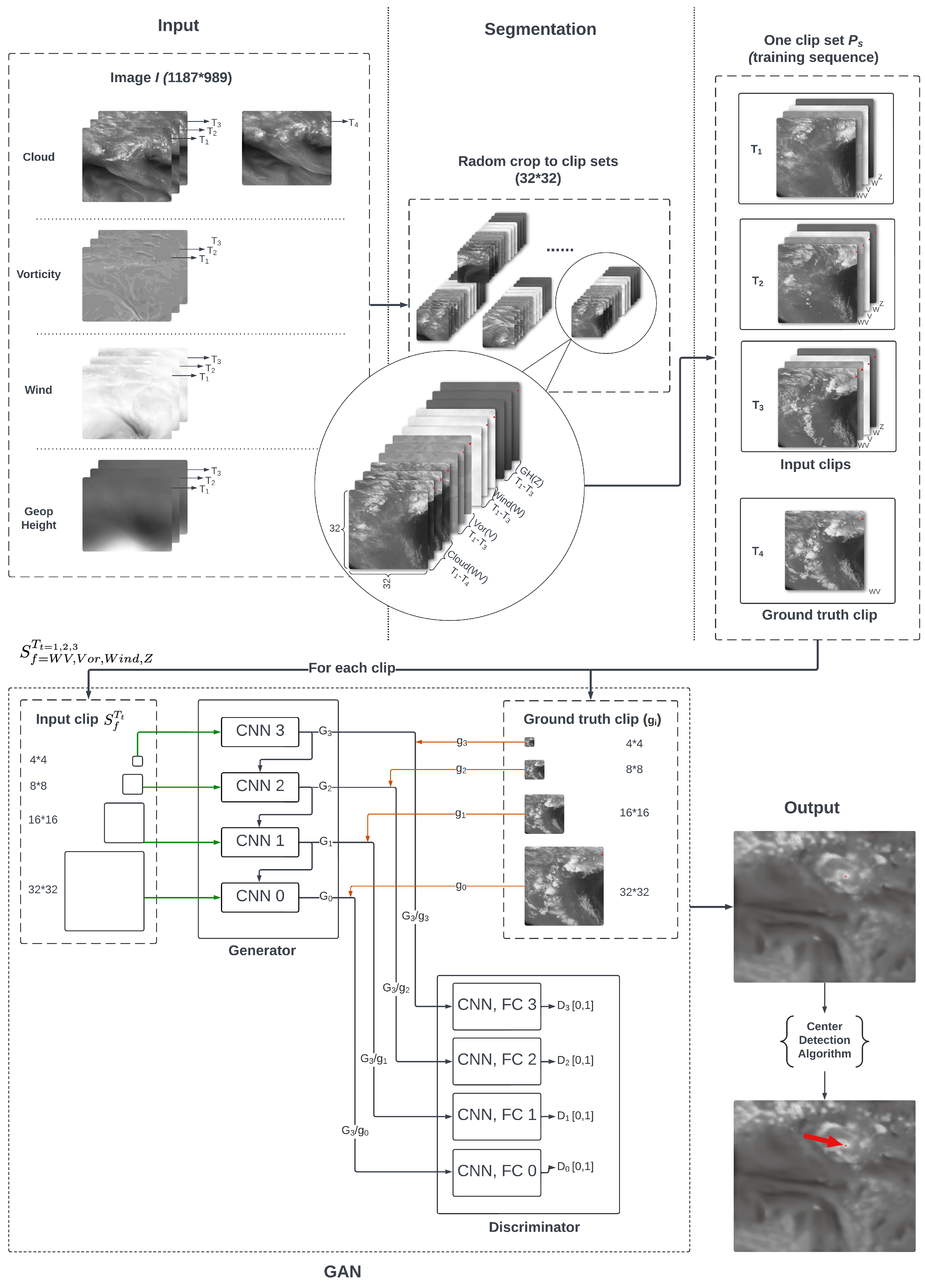
2.2.1. Input Data and Segmentation Algorithm

The input images consist of four distinct meteorological features: Cloud (WV), Vorticity (Vor), Wind, and Geopotential Height (Z). These images use equal-latitude and longitude grids for the Australian region (100–160°E, 0–50°S). All of these features were captured at three consecutive time steps (T1, T2, T3). An additional time step (T4) is only included for Cloud (WV), serving as the ground truth for training. Cloud (WV) is chosen as the target variable due to its close correlation with TC center characteristics, making it a critical feature for tracking and forecasting [27]. In contrast, other features such as vorticity, wind, and geopotential height are excluded at T4, as their primary role is to provide contextual meteorological information rather than serving as the primary targets for prediction. Overall, the T4 image provides the “future state” of the TC’s cloud distribution at the next time step, distinct from T1–T3, which represents historical progression. This distinction allows the model to learn the temporal evolution of the TC from T1–T3 and use it to predict T4. During training, the T4 image acts as the supervisory signal (ground truth) to optimize the model’s parameters. All input images are preprocessed to remove redundant information, such as borders, and resized into a resolution of $1187\times 989$, ensuring consistent and efficient input for the model. This preprocessing step ensures that the data capture the essential dynamics of the TC while excluding unnecessary noise.

In the subsequent segmentation step, the input images are randomly cropped into smaller regions. The purpose of the segmentation is to extract meaningful spatial information across different meteorological features and time steps. First, the algorithm selects three consecutive time steps and randomly crops a $32\times 32$ region from each image group (WV, Vor, Wind and Z). Second, the L2-norm difference between consecutive time steps is calculated to detect the significant variation in the region. If a meaningful difference is found, the cropped region is retained; otherwise, the region is discarded. This segmentation is performed for each TC, and the retained cropped regions are used as input to the GAN. It is important to note that while the T4 images also undergo the segmentation process mentioned above, they differ from the T1–T3 images in that they do not participate in the generator training. Instead, they are used as input to the discriminator and, together with the T4 images generated by the generator, are used to train the discriminator. Algorithm 1 provides specific details.

Algorithm 1 Segmentation algorithm for TCs prediction.

Require: TCs images I at different time steps $T_t$, where for $F_{WV}$, $t=1,2,3,4$; for $F_{Vor},F_{Wind},F_Z$, $t=1,2,3$ Require: Number of feature subsets $F_f$, where $f=WV,Vor,Wind,Z$ Ensure: Preprocessed image clips $P_s$ with $F_{WV}^{T_4}$ included  1:  $P_s\leftarrow \left[\right]$  2:  for each TC dataset $I_i$ do  3:    for $f=WV,Vor,Wind,Z$ do  4:      for $T_1, T_2, T_3$ consecutive frames do  5:        Randomly sample a $32\times 32$ region from $T_1,T_2,T_3$  6:        if $L2\_norm(T_1,T_2)>ϵ$ or $L2\_norm(T_2,T_3)>ϵ$ then  7:         Retain the cropped region  8:        else  9:         Continue sampling until meaningful variation is found (max 100 trials) 10:        end if 11:      end for 12:    end for 13:    Append corresponding $F_{WV}^{T_4}$ region to $P_s$ to 14:    Append selected regions from $T_1, T_2, T_3$ and $F_{WV}^{T_4}$ to $P_s$ 15:  end for 16:  return $P_s$

2.2.2. Multi-Scale GAN

The generator of multi-scale GAN is composed of four CNN layers. For each clip obtained by the segmentation algorithm, a hierarchical set of images at multiple resolutions ($4\times 4$, $8\times 8$, $16\times 16$, and $32\times 32$) is generated and used as input to the generator. The discriminator, composed of 4 convolutional layers followed by a fully connected (FC) layer, evaluates the generated images at each resolution by comparing them to the corresponding ground truth (WV at T4). Through convolutional operations, the discriminator repeatedly extracts hierarchical features from the input data at different resolutions, capturing both global patterns and local details to improve its representation of complex TC structures. The fully connected layer aggregates these extracted features and maps them to a final output prediction, which is constrained to a range between 0 and 1 by the sigmoid activation function. This output represents the probability that the input data are real and provides feedback to guide the generator’s training process. The generator is iteratively refined to minimize prediction errors, thereby producing more accurate results. Ultimately, the GAN system generates a predicted cloud image (WV) for time T4, representing the cyclone’s state three hours into the future.

Our model uses a combined loss function, where the total loss function (1) combines three components. The model minimizes the loss during training to obtain generated images that are indistinguishable from the discriminator.

$$L_{\mathrm{total}}={\lambda }_{\mathrm{lp}}·L_{\mathrm{lp}}+{\lambda }_{\mathrm{gdl}}·L_{\mathrm{gdl}}+{\lambda }_{\mathrm{adv}}·L_{\mathrm{adv}}$$

(1)

where $L_{lp}$ is the pixel loss (or Lp loss), $L_{gdl}$ is the gradient difference loss, $L_{adv}$ is the adversarial loss, and ${\lambda }_{lp}, {\lambda }_{gdl}, {\lambda }_{adv}$ are the corresponding weights.

The pixel-wise loss Equation (2) follows:

$$L_{lp}={\displaystyle \frac{1}{N}}\sum _{i=1}^N\sum _{\mathrm{pixels}}{\left|{\widehat{I}}_i-I_i\right|}^{l_{\mathrm{num}}}$$

(2)

where N is the number of frames, ${\widehat{I}}_i$ is the generated frame, $I_i$ is the corresponding ground truth frame, and $l_{num}$ represents the norm order (default $l_{num}=2$, making it an L2 loss).

For GDL loss (Gradient Difference Loss),

$$L_{\mathrm{gdl}}={\displaystyle \frac{1}{N}}\sum _{i=1}^N\sum _{\mathrm{pixels}}\left({\left|{\nabla }_x{\widehat{I}}_i-{\nabla }_x{I}_i\right|}^{\alpha }+{\left|{\nabla }_y{\widehat{I}}_i-{\nabla }_y{I}_i\right|}^{\alpha }\right)$$

(3)

where ${\nabla }_x$ and ${\nabla }_y$ represent the gradients in the x and y directions, respectively, and $\alpha$ controls the strength of the gradient difference (default $\alpha =2$).

The adversarial loss Equation (4) follows:

$$L_{\mathrm{adv}}={\displaystyle \frac{1}{N}}\sum _{i=1}^N\mathrm{BCE}(p_i,1)$$

(4)

where $p_i$ is the discriminator’s prediction for the generated image, and $BCE(p_i, 1)$ is the binary cross-entropy loss with a target value of 1, indicating that the generator aims for the discriminator to classify the generated image as real.

2.2.3. Center Detection Algorithm

In most cases, the GAN’s images generate a distinct red point. However, in certain instances, multiple potential centers with varying red intensities emerge, which can be interpreted as reflecting the model’s prediction confidence [19]. This issue becomes more pronounced when making predictions based on anomalous satellite imagery. For instance, false TC centers may appear along the edges of horizontal line artifacts (Figure 2a) or within areas of missing data (Figure 2b). Detecting the most probable TC center is the primary function of the center detection algorithm. The following is the pseudo-code of our center detection Algorithm 2.

Algorithm 2 Center detection algorithm.

Require: Image I, Previous Center $C_{\mathrm{last}}$ (optional) Ensure: Coordinates of the detected red point $(C_x,C_y)$  1:  Convert I to HSV: $I_{\mathrm{HSV}}=\mathrm{HSV}\left(I\right)$  2:  Create red masks: $\mathrm{mask}=\mathrm{MaskRed}\left(I_{\mathrm{HSV}}\right)$  3:  Clean mask using morphological operations  4:  Find contours $\left\{c_i\right\}$ in mask  5:  if $\left\{c_i\right\}=\varnothing$ then  6:     return $(\mathrm{None}, \mathrm{None})$  7:  end if  8:  Initialize: $C_{\mathrm{reddest}}=\mathrm{None}$, $C_{\mathrm{closest}}=\mathrm{None}$  9:  max_mean_val $\leftarrow 0$, min_distance $\leftarrow \infty$ 10:  for each $c_i$ do 11:    Compute mean saturation: mean_vali $={\displaystyle \frac{1}{|c_i|}}{\sum }_{p\in c_i}S\left(p\right)$ 12:    Compute centroid: $(c_x,c_y)=\left({\displaystyle \frac{{\sum }_{p\in c_i}{x}_p}{|c_i|}},{\displaystyle \frac{{\sum }_{p\in c_i}{y}_p}{|c_i|}}\right)$ 13:    if $C_{\mathrm{last}} \ne \text{None}$ then 14:     Compute distance: $d_i=\sqrt{{(c_x-C_{\mathrm{last},x})}^2+{(c_y-C_{\mathrm{last},y})}^2}$ 15:     if $d_i<$ min_distance then 16:      $C_{\mathrm{closest}}\leftarrow c_i$, min_distance $\leftarrow d_i$ 17:     end if 18:    end if 19:    if mean_vali > max_mean_val then 20:     $C_{\mathrm{reddest}}\leftarrow c_i$, max_mean_val ← mean_vali 21:    end if 22:  end for 23:  $C_{\mathrm{chosen}}\leftarrow \left\{\begin{array}{cc}{C}_{\mathrm{closest}},\hfill & \text{if min\_distance}\le 100\hfill \\ C_{\mathrm{reddest}},\hfill & \text{otherwise}\hfill \end{array}\right.$ 24:  if $C_{\mathrm{chosen}}\ne \mathrm{None}$  then 25:    Compute and return centroid: $(C_x, C_y)$ 26:  else 27:    return $(\mathrm{None}, \mathrm{None})$ 28:  end if

The algorithm detects the center of a TC using two red point conditions. One criterion is to identify the reddest point. We accomplish this by defining a hue range mask, applying morphological operations to reduce noise, identifying all red areas, calculating the average saturation of each red point, and selecting the point with the highest average saturation as the possible TC center. The other criterion is to choose the nearest red point within a specified threshold based on its distance from the previous TC center. This threshold is determined by considering the historical speed of the currently predicted TC and the maximum possible displacement of the fastest-moving tropical cyclone in the southern hemisphere within a 3 h period (about 500 km in 3 h, 167 km/h) [40], serving as a prioritized search window. If the predicted TC center is found within the prioritized search window, it is selected. Otherwise, the reddest point in the entire generated image is chosen. Finally, the centroid of the selected point is calculated and returned as the coordinates of the TC center.

2.3. Model Performance Evaluation

To evaluate the performance of our model, the absolute error is calculated for each prediction, which represents the discrepancy between the predicted TC center position and the actual TC center position. As the satellite images used for model training and testing have been flattened using an equidistant longitude and latitude projection algorithm, we map the pixel coordinates of the TC center on the predicted image to the longitude and latitude coordinates of the earth’s surface using the Harvard formula and then calculate the prediction absolute error. The specific Formula (5) is as follows.

$$E=2R·arcsin\left(\sqrt{{sin}^2\left({\displaystyle \frac{\Delta \varphi }{2}}\right)+cos\left({\varphi }_1\right)·cos\left({\varphi }_2\right)·{sin}^2\left({\displaystyle \frac{\Delta \lambda }{2}}\right)}\right)$$

(5)

where E is the distance between two points (in kilometers), R is the Earth’s mean radius (6371.0 km), ${\varphi }_1, {\varphi }_2$ are the latitudes of the two points (in radians), ${\lambda }_1, {\lambda }_2$ are the longitudes of the two points (in radians), $\Delta \varphi ={\varphi }_2-{\varphi }_1$ is the difference in latitudes, and $\Delta \lambda ={\lambda }_2-{\lambda }_1$ is the difference in longitudes.

3. Results

3.1. Model Performance over Ocean and Land, Best Track and Extended Track and Its Robustness

The prediction error distribution of all TC center points is shown in Figure 3. This figure presents the error distribution and pairwise relationships of error values for TCs over ocean and land in the best track and in the extended track, respectively. The diagonal plots (panels a, f, k, p) illustrate the error frequency distributions, which are primarily concentrated in the lower range, forming near-normal distributions. This clustering in the lower-left corner and the bell-shaped curves demonstrate that the model predictions are generally stable and reliable across most TC track types. Additionally, the distributions exhibit a slight left skew, indicating that the model consistently produces low error values with only a few outliers at higher error ranges. This skewness highlights the model’s strong and stable performance with most error values remaining well contained and significant deviations being minimal.

When comparing the different track types, TCs over land and in the extended track show broader spreads compared to TCs over ocean and in the best track, which means the model encounters more challenges when dealing with complex land interactions and fewer organized TC remnants. This can be observed by comparing specific panels. For example, the prediction errors for ocean segments in the best track (panels d and m) are more concentrated and skewed toward smaller error values compared to those for land segments in the best track (panels c and i) and ocean segments in the extended track (panels h and n).

The average error and standard deviation of TC predictions for each year from 2015 to 2020 are shown in

Table 2. Average error (km) and standard deviation (km) by category and year.

Type			2015	2016	2017	2018	2019	2020	2015–2020
All		Ave.Er	47.2	45.6	36.6	37.8	40.8	39.2	41.0
		hlstd	41.4	51.1	38.2	48.2	29.1	42.9	42.8
Surface	Ocean	Ave.Er	38.5	40.7	36.7	38.3	37.7	31.1	37.8
		std	40.1	47.9	35.9	43.8	27.7	44.2	39.8
	Land	Ave.Er	49.4	67.4	41.9	41.5	41.7	42.8	47.5
		std	42.7	50.9	42.9	60.0	32.7	42.1	47.0
Track	Best	Ave.Er	31.5	30.8	31.0	33.5	37.0	24.6	32.0
		std	26.4	30.3	30.7	45.2	27.1	17.7	33.0
	Extended	Ave.Er	82.5	90.9	76.2	70.0	57.6	74.2	78.4
		std	58.1	56.0	49.4	52.6	41.5	60.9	55.3

. It is clear that the average error over ocean (37.8 km) is lower than over land (47.5 km), and it is also much smaller than the forecast error (95.6 km) from the AI model using cloud image only [10,19]. The forecast error difference between ocean and land may be attributed to terrain interference and more significant forecast uncertainty when the storm transitions over land. Our error over land (47.5 km) is much lower than the error (140 km) in the comparative study [19]. In addition, the results indicate that the average error and standard deviation of TCs over the tested six years exhibit minimal fluctuation across different TC types, remaining within approximately 60 km for nearly all cases except for the extended tracks. This consistency highlights the model’s stability.

Details of the forecasts for all 28 TCs from 2015 to 2020 are shown in

Table 3. Average errors (km) for TCs over ocean and land in best track and extended track. “NaN” means no data.

TC ID	Surface		Track		All
	Ocean	Land	Best	Extended
2015045S12145-LAM	18.1	47.2	24.7	63.1	38.6
2015047S15152-MARCIA	39.7	36.7	35.5	45.2	37.6
2015068S12151-NATHAN	62.7	88.6	30.4	120.9	40.6
2015068S14113-OLWYN	67.6	105.0	67.9	104.4	62.6
2015117S12115-QUANG	38.7	68.9	21.9	132.5	56.0
2015355S16136-NOT_NAMED	NaN	57.6	33.4	81.8	47.6
2016027S13119-STAN	94.6	127.1	69.7	152.0	61.1
2016074S16137-NOT_NAMED	24.9	41.0	23.3	60.3	32.4
2016353S11130-NOT_NAMED	89.5	50.3	27.8	111.9	61.0
2016354S15116-YVETTE	29.2	12.7	24.5	5.5	28.1
2017026S16127-NOT_NAMED	30.3	27.6	29.0	NaN	30.2
2017046S17137-ALFRED	55.3	61.9	30.9	86.2	52.0
2017060S09139-BLANCHE	57.6	39.9	28.7	68.8	44.1
2017079S13122-NOT_NAMED	22.8	51.4	36.0	53.6	34.2
2017081S13152-DEBBIE	108.7	48.6	43.6	178.9	44.4
2017096S08135-NOT_NAMED	41.1	20.6	26.8	49.2	32.8
2017360S15124-HILDA	12.8	38.2	12.2	64.6	18.8
2018007S13129-JOYCE	31.8	28.2	23.1	45.5	26.4
2018044S10133-KELVIN	44.5	50.8	20.1	75.2	34.3
2018074S09130-MARCUS	98.8	32.0	33.8	162.0	48.2
2018079S08137-NORA	43.5	31.7	25.9	49.3	35.8
2018336S14154-OWEN	43.5	106.6	69.9	53.6	42.8
2018365S13140-PENNY	37.7	39.4	33.1	50.2	39.3
2019077S13146-TREVOR	18.9	60.1	25.3	88.7	27.1
2019132S16159-ANN	54.0	66.6	60.3	NaN	54.6
2020006S16121-BLAKE	21.2	35.8	22.5	47.6	32.8
2020037S17121-DAMIEN	105.9	55.0	21.0	139.9	40.2
2020055S15139-ESTHER	24.7	55.0	28.1	78.5	44.6

. From the table, we can find that there are three TCs with errors greater than 100 km over land, namely 2015068S14113-OLWYN, 2016027S13119-STAN, and 2018336S14154-OWEN. Observing their path diagrams (Figure 4), we can find that all of these TC’s moving speeds accelerated after landing, and TC OWEN’s trajectory was complex and looping at the same time, making it difficult for the model to predict their centers.

Figure 5 illustrates the forecast error difference between TCs in the best track and those in the extended track both after the TC made landfall. The model shows a significantly lower error in the best track than in the extended track. This discrepancy can be attributed to the fact that TCs in the extended track are mostly TC remnants. They are less organized and often split into multiple convection centers unlike the more coherent and robust TC systems observed in the best track. Additionally, some TCs, such as Olwyn and Owen, did not have an extended track after landfall, so only their best track data are shown in the figure. Finally, it should be mentioned that the results differ significantly from Table 2, since TC points over the ocean are not taken into account in this computation.

3.2. Model Performance for TCs with Abnormal Satellite Imagery

Among the 28 TCs from 2015 to 2020 in our testing dataset, five TCs contain abnormal satellite images. Of these, four TCs (2017026S16127-NOT_NAMED, 2017079S13122-NOT_NAMED, 2017081S13152-DEBBIE, and 2017096S08135-NOT_NAMED) have horizontal line artifacts in all track points, as illustrated in Figure 2a. Additionally, TC 2018044S10133-KELVIN includes blank satellite images for ten consecutive track points out of a total of 86 points, as shown in Figure 2b. Prediction errors for these TCs using our method and other existing methods are summarized in

Table 4. Absolute error (km) using different methods on TCs with abnormal satellite imagery.

TC ID	Total Points	Abnormal	Absolute Error (km)
			[10,19]	Ours
2017026S16127-NOT_NAMED	50	49	3465.3	30.2
2017079S13122-NOT_NAMED	48	48	2012.5	34.2
2017081S13152-DEBBIE	83	83	3451.6	44.4
2017096S08135-NOT_NAMED	83	83	3713.6	32.8
2018044S10133-KELVIN	86	10	623.8	34.3
Average	70	55	2653.4	35.2

. To ensure a fair comparison, both our model and the approach from Ruttgers et al. [10,19] were trained and tested on the same dataset, which includes multiple meteorological parameters. Table 4 is with a focus on assessing their performance in handling cases with anomalous satellite images. The method proposed by Ruttgers et al. produces an average error of 2653.4 km, while our method achieves an average absolute error of only 35.2 km. This significant reduction in error highlights the robustness of our approach and explains why TCs with abnormal satellite imagery have typically been excluded from previous studies.

In contrast to the substantial errors produced by other methods, Table 4 demonstrates the exceptional robustness of our model in handling abnormal satellite imagery. Here, we take 2017026S16127-NOT_NAMED at 2017012612 UTC and 2018044S10133-KELVIN at 2018021309UTC as examples to show our model’s TC detection for TCs with abnormal satellite imagery (Figure 6). As we can see, our model accurately pinpoints the TC center (Figure 6b,d) when satellite have horizontal line artifacts (Figure 6a) or blank artifacts (Figure 6c). This capability underscores the strength of our approach in leveraging diverse input features and the center detection algorithm to overcome the limitations posed by abnormal or incomplete satellite imagery, achieving significantly higher accuracy and reliability.

3.3. Case Study

TC 2015045S12145-LAM, the first TC in our testing dataset in 2015–2020, is taken as an example to show the forecast of our model in Figure 7. TC LAM has two landfall points, one in North Queensland and the other in the North Northern Territory, which includes two periods over ocean and land, respectively. The best track record for TC LAM consists of 56 track points, each representing a three-hour interval (time points 1–56). After the best track record ends, TC LAM continues in the extended track for an additional 37 track points (time points 57–93), surviving for another 4.5 days. From Figure 7, it is evident that our track prediction closely aligns with the actual path, particularly when the TC is over the ocean. After TC LAM moves onto the mainland, the prediction begins to show more noticeable deviations, especially during the final dissipation stage of the TC (time points 73–93). The average error for the entire path is 38.6 km, while it is 18.1 km over ocean and 47.2 km over land, respectively. In addition, the error in the extended track (63.1 km) is larger than in the best track (24.7 km).

There are still some cases where our model shows considerable predicting mistakes, even if its average error is far lower than that of other studies. Figure 8 shows two points when TC LAM over the ocean at 201502182100 UTC and over land at 201502251200 UTC with forecast errors of 27.3 km and 151.6 km, respectively. The left panels show the actual satellite cloud imagery for these two points, while the right panels present the predicted images. As we can see, the cloud structure of the TC is well organized, with a distinct eye when the TC is over the ocean, which makes identifying the TC center straightforward. In contrast, the cloud patterns are disorganized when the TC is over land, making it difficult for the model to predict the TC center correctly. This disparity explains the challenges of predicting TC centers over land and the limited progress in this aspect. However, our model demonstrates the ability to achieve higher prediction accuracy for TCs over land than others. This capability stems from our model’s ability to learn from diverse input features. For instance, while the cloud structure of TC LAM at 201502251200 UTC is poorly organized, additional dynamical and structural cues are available in the vorticity, geopotential height, and wind speed fields at 700 hPa (Figure 9). The 700 hPa level is often used in TC studies because it represents the mid-tropospheric vortex, which remains coherent even when surface features are disrupted. The vorticity field highlights the strongest rotational center, the geopotential height field provides information on the synoptic-scale structure, and the wind field constrains circulation patterns. These combined inputs serve as supplementary signals for center identification, particularly in mid- and high-latitude TCs, where satellite imagery alone may not be sufficient. Our model effectively learns and integrates these different sources of information, allowing it to make more accurate predictions in challenging cases.

4. Discussion

As demonstrated above, our model exhibits high accuracy in tracking TCs and their remnants over both ocean and land, even for TCs with abnormal satellite imagery. However, there are areas for improvement in the next step.

4.1. Accuracy over Land and in the Extended Tracks

The model demonstrates improved prediction accuracy for TC paths over land compared to other studies, but it still lags behind the accuracy for TC tracks over ocean. In addition, the predictions for the extended track exhibit significantly lower accuracy compared to the best track segments. These discrepancies may arise due to the complex and heterogeneous surface properties of land, not well-organized cloud structures, and may fragment into multiple convective centers in post-TC systems. To address these challenges, improvements can be made by enhancing the model’s processing capabilities through the inclusion of targeted data training to better capture land interaction dynamics. Additionally, domain-specific fine tuning or transfer learning from similar land-based phenomena, the integration of advanced reanalysis datasets with higher temporal and spatial resolution, and the implementation of attention mechanisms to focus on subtle features in extended tracks could further refine the model’s performance.

4.2. Challenges with Rapid TC Movement and Complex Trajectories

The model’s performance decreases when TCs exhibit sudden accelerations or follow highly complex, intertwined paths. These scenarios introduce nonlinear and nonstationary behaviors that are challenging for the model to predict. Potential solutions include enriching the training dataset with similar rapid or complex trajectories to improve the model’s generalization. Additionally, hybrid models combining physical constraints (e.g., derived from TC dynamics) with data-driven approaches could help capture these extreme variations more accurately. Incorporating temporal attention mechanisms or recurrent neural networks with long memory capabilities might also enhance the model’s ability to understand and predict abrupt changes.

4.3. Segmentation Algorithm

The segmentation algorithm used in this study was custom-developed, which offered flexibility in tailoring it to specific data and task requirements. However, specialized pre-trained models like U-Net or DeepLabV3+ could provide significant advantages in terms of segmentation precision and robustness. These models leverage large-scale datasets and are optimized for diverse scenarios, making them more generalizable. While custom algorithms are easier to adapt and computationally lighter, pre-trained models excel in extracting detailed features and handling complex segmentation tasks. Future studies could evaluate the trade-offs between computational efficiency and segmentation quality by integrating such pre-trained models.

4.4. Handling Abnormal Satellite Image

While the current model addresses abnormal meteorological data by incorporating additional meteorological information and a center detection mechanism, future work could benefit from the integration of dedicated anomaly detection algorithms. Techniques such as autoencoders or GAN-based anomaly detectors could identify and reconstruct anomalous regions more effectively. However, these approaches require the careful manual curation of training data, as anomalies need to be identified and labeled, which is labor-intensive. Additionally, the reliance on unsupervised learning may introduce uncertainties. Developing automated anomaly detection pipelines with minimal manual intervention could make this process more feasible for large-scale datasets.

4.5. Model Output Cloud Image

The model accurately generates TC centers, but the accompanying cloud imagery appears blurred. This may be related to the relatively high resolution of the input images (1187 × 989), which might dilute finer-scale features during multi-scale feature extraction. In the future, if a clear and accurate cloud map is required (e.g., TC rainfall forecast from cloud map), it might involve using higher-resolution feature maps, integrating feature extraction at larger scales, or employing a super-resolution module in the generator to refine output quality.

5. Conclusions

Compared to previous studies relying solely on satellite imagery, this study developed a novel GAN multi-source prediction model that synergistically integrates satellite imagery, wind speed, geopotential height, and vorticity data. This approach enables the high-precision tracking of TC trajectories over both ocean and land. Our model surpasses the limitations of best-track data by accurately tracing post-TC locations until complete dissipation, thereby capturing the full lifecycle of landfalling TCs and enabling a comprehensive understanding of their overall impacts.

The model demonstrates strong predictive performance and generalization capabilities even when trained on a limited dataset. It was trained on 14 randomly selected TCs and tested on all 28 TCs from 2015 to 2020, including five cases with significant anomalies in satellite imagery. The results indicate that despite challenges such as complex ocean–land trajectories, weak features during dissipating stages, and interference from anomalous data, the model maintains promising predictive performance with a consistently low absolute error of 41.0 km. Specifically, the model achieved high prediction accuracy for best track segments, with an average error of 32.0 km, while predictions for extended segments exhibited relatively larger errors of 78.4 km. Additionally, the prediction error over land (47.5 km) was higher than that over the ocean (37.8 km), as summarized in Table 2. Moreover, both the errors and their standard deviations remained stable over the six-year testing period, demonstrating the model’s robustness and the strong potential of the GAN-based approach for tracking and predicting TCs over both ocean and land, including their progression further inland. For the five TCs with anomalous satellite observations, the model maintained high accuracy, achieving a prediction error of 35.2 km, which is a scenario often overlooked or inadequately addressed by other approaches.

Furthermore, incorporating numerical model outputs or reanalysis into the AI model establishes a robust foundation for TC track identification, particularly when portions of observational satellite data are unavailable. This study offers reliable technical support and significant value for the study for the automatic detection of TCs and their remnants on a global scale both in historical contexts and under future warming scenarios, which will be explored in our next step.

References

1. Wang, S.; Toumi, R. More tropical cyclones are striking coasts with major intensities at landfall. Sci. Rep. 2022, 12, 5236. [Google Scholar] [CrossRef] [PubMed]
2. Chen, R.; Zhang, W.; Wang, X. Machine learning in tropical cyclone forecast modeling: A review. Atmosphere 2020, 11, 676. [Google Scholar] [CrossRef]
3. Klotzbach, P.; Blake, E.; Camp, J.; Caron, L.P.; Chan, J.C.; Kang, N.Y.; Kuleshov, Y.; Lee, S.M.; Murakami, H.; Saunders, M.; et al. Seasonal tropical cyclone forecasting. Trop. Cyclone Res. Rev. 2019, 8, 134–149. [Google Scholar] [CrossRef]
4. Kalnay, E. Atmospheric Modeling, Data Assimilation and Predictability; Cambridge University Press: Cambridge, UK, 2003; Volume 341. [Google Scholar]
5. Roy, C.; Kovordányi, R. Tropical cyclone track forecasting techniques―A review. Atmos. Res. 2012, 104, 40–69. [Google Scholar] [CrossRef]
6. Long, T.; Fu, J.; Tong, B.; Chan, P.; He, Y. Identification of tropical cyclone centre based on satellite images via deep learning techniques. Int. J. Climatol. 2022, 42, 10373–10386. [Google Scholar] [CrossRef]
7. Wang, Z.; Zhao, J.; Huang, H.; Wang, X. A review on the application of machine learning methods in tropical cyclone forecasting. Front. Earth Sci. 2022, 10, 902596. [Google Scholar] [CrossRef]
8. Wimmers, A.; Velden, C.; Cossuth, J.H. Using deep learning to estimate tropical cyclone intensity from satellite passive microwave imagery. Mon. Weather Rev. 2019, 147, 2261–2282. [Google Scholar] [CrossRef]
9. Zhang, C.J.; Wang, X.J.; Ma, L.M.; Lu, X.Q. Tropical cyclone intensity classification and estimation using infrared satellite images with deep learning. IEEE J. Sel. Top. Appl. Earth Obs. Remote Sens. 2021, 14, 2070–2086. [Google Scholar] [CrossRef]
10. Rüttgers, M.; Jeon, S.; Lee, S.; You, D. Prediction of typhoon track and intensity using a generative adversarial network with observational and meteorological data. IEEE Access 2022, 10, 48434–48446. [Google Scholar] [CrossRef]
11. Gan, S.; Fu, J.; Zhao, G.; Chan, P.; He, Y. Short-term prediction of tropical cyclone track and intensity via four mainstream deep learning techniques. J. Wind Eng. Ind. Aerodyn. 2024, 244, 105633. [Google Scholar] [CrossRef]
12. Dorffner, G. Neural networks for time series processing. Neural Netw. World 1996, 6, 447–468. [Google Scholar]
13. Hochreiter, S. Long Short-term Memory. Neural Comput. 1997, 9, 1735–1780. [Google Scholar] [CrossRef]
14. Alemany, S.; Beltran, J.; Perez, A.; Ganzfried, S. Predicting hurricane trajectories using a recurrent neural network. In Proceedings of the AAAI Conference on Artificial Intelligence, Honolulu, HI, USA, 27 January 2019–1 February 2019; Volume 33, pp. 468–475. [Google Scholar]
15. LeCun, Y.; Boser, B.; Denker, J.S.; Henderson, D.; Howard, R.E.; Hubbard, W.; Jackel, L.D. Backpropagation applied to handwritten zip code recognition. Neural Comput. 1989, 1, 541–551. [Google Scholar] [CrossRef]
16. Wang, C.; Xu, Q.; Li, X.; Cheng, Y. CNN-based tropical cyclone track forecasting from satellite infrared images. In Proceedings of the IGARSS 2020–2020 IEEE International Geoscience and Remote Sensing Symposium, Waikoloa, HI, USA, 26 September–2 October 2020; IEEE: Piscataway, NJ, USA, 2020; pp. 5811–5814. [Google Scholar]
17. Tong, B.; Wang, X.; Fu, J.; Chan, P.; He, Y. Short-term prediction of the intensity and track of tropical cyclone via ConvLSTM model. J. Wind Eng. Ind. Aerodyn. 2022, 226, 105026. [Google Scholar] [CrossRef]
18. Goodfellow, I.; Pouget-Abadie, J.; Mirza, M.; Xu, B.; Warde-Farley, D.; Ozair, S.; Courville, A.; Bengio, Y. Generative adversarial nets. In Advances in Neural Information Processing Systems, Proceedings of the NIPS’14: Proceedings of the 28th International Conference on Neural Information Processing Systems, Montreal, QC, Canada, 8–13 December 2014; MIT Press: Cambridge, MA, USA, 2014; Volume 27. [Google Scholar]
19. Rüttgers, M.; Lee, S.; Jeon, S.; You, D. Prediction of a typhoon track using a generative adversarial network and satellite images. Sci. Rep. 2019, 9, 6057. [Google Scholar] [CrossRef]
20. Huang, C.; Bai, C.; Chan, S.; Zhang, J.; Wu, Y. MGTCF: Multi-generator tropical cyclone forecasting with heterogeneous meteorological data. In Proceedings of the AAAI Conference on Artificial Intelligence, Washington, DC, USA, 7–14 February 2023; Volume 37, pp. 5096–5104. [Google Scholar]
21. Vaswani, A. Attention is all you need. In Advances in Neural Information Processing Systems, Proceedings of the 31st Annual Conference on Neural Information Processing Systems (NIPS 2017), Long Beach, CA, USA, 4–9 December 2017; Curran Associates Inc.: Red Hook, NY, USA, 2017. [Google Scholar]
22. Bi, K.; Xie, L.; Zhang, H.; Chen, X.; Gu, X.; Tian, Q. Accurate medium-range global weather forecasting with 3D neural networks. Nature 2023, 619, 533–538. [Google Scholar] [CrossRef]
23. Lian, J.; Dong, P.; Zhang, Y.; Pan, J.; Liu, K. A novel data-driven tropical cyclone track prediction model based on CNN and GRU with multi-dimensional feature selection. IEEE Access 2020, 8, 97114–97128. [Google Scholar] [CrossRef]
24. Moradi Kordmahalleh, M.; Gorji Sefidmazgi, M.; Homaifar, A. A sparse recurrent neural network for trajectory prediction of atlantic hurricanes. In Proceedings of the Genetic and Evolutionary Computation Conference, Denver, CO, USA, 20–24 July 2016; pp. 957–964. [Google Scholar]
25. Takaya, Y.; Caron, L.P.; Blake, E.; Bonnardot, F.; Bruneau, N.; Camp, J.; Chan, J.; Gregory, P.; Jones, J.J.; Kang, N.; et al. Recent advances in seasonal and multi-annual tropical cyclone forecasting. Trop. Cyclone Res. Rev. 2023, 12, 182–199. [Google Scholar] [CrossRef]
26. Bi, K.; Xie, L.; Zhang, H.; Chen, X.; Gu, X.; Tian, Q. Pangu-weather: A 3d high-resolution model for fast and accurate global weather forecast. arXiv 2022, arXiv:2211.02556. [Google Scholar]
27. Olander, T.L.; Velden, C.S. The advanced Dvorak technique (ADT) for estimating tropical cyclone intensity: Update and new capabilities. Weather Forecast. 2019, 34, 905–922. [Google Scholar] [CrossRef]
28. Shen, H.; Li, X.; Cheng, Q.; Zeng, C.; Yang, G.; Li, H.; Zhang, L. Missing information reconstruction of remote sensing data: A technical review. IEEE Geosci. Remote Sens. Mag. 2015, 3, 61–85. [Google Scholar] [CrossRef]
29. Wang, P.; Bayram, B.; Sertel, E. A comprehensive review on deep learning based remote sensing image super-resolution methods. Earth-Sci. Rev. 2022, 232, 104110. [Google Scholar] [CrossRef]
30. Shen, H.; Wu, J.; Cheng, Q.; Aihemaiti, M.; Zhang, C.; Li, Z. A spatiotemporal fusion based cloud removal method for remote sensing images with land cover changes. IEEE J. Sel. Top. Appl. Earth Obs. Remote Sens. 2019, 12, 862–874. [Google Scholar] [CrossRef]
31. Guillemot, C.; Le Meur, O. Image inpainting: Overview and recent advances. IEEE Signal Process. Mag. 2013, 31, 127–144. [Google Scholar] [CrossRef]
32. Tang, Z.; Amatulli, G.; Pellikka, P.K.; Heiskanen, J. Spectral temporal information for missing data reconstruction (stimdr) of landsat reflectance time series. Remote Sens. 2021, 14, 172. [Google Scholar] [CrossRef]
33. Liu, W.; Jiang, Y.; Wang, J.; Zhang, G.; Li, D.; Song, H.; Yang, Y.; Huang, X.; Li, X. Global and Local Dual Fusion Network for Large-Ratio Cloud Occlusion Missing Information Reconstruction of a High-Resolution Remote Sensing Image. IEEE Geosci. Remote Sens. Lett. 2024, 21, 5001705. [Google Scholar] [CrossRef]
34. Xu, H.; Tang, X.; Ai, B.; Gao, X.; Yang, F.; Wen, Z. Missing data reconstruction in VHR images based on progressive structure prediction and texture generation. ISPRS J. Photogramm. Remote Sens. 2021, 171, 266–277. [Google Scholar] [CrossRef]
35. Long, C.; Li, X.; Jing, Y.; Shen, H. Bishift networks for thick cloud removal with multitemporal remote sensing images. Int. J. Intell. Syst. 2023, 2023, 9953198. [Google Scholar] [CrossRef]
36. Li, Y.; Wei, F.; Zhang, Y.; Chen, W.; Ma, J. HS2P: Hierarchical spectral and structure-preserving fusion network for multimodal remote sensing image cloud and shadow removal. Inf. Fusion 2023, 94, 215–228. [Google Scholar] [CrossRef]
37. Deng, D.; Ritchie, E. Tropical cyclone rainfall enhancement following landfalling over Australia-Part III. In Proceedings of the American Geophysical Union Fall Meeting 2023, San Francisco, CA, USA, 11–15 December 2023; Volume 2023, p. A54F-06. [Google Scholar]
38. Deng, D. A Physical-based Semi-Automatic Algorithm for Post-Tropical Cyclone Identification and Tracking in Australia. Remote Sens. 2025, 17, 539. [Google Scholar] [CrossRef]
39. Deng, D.; Ritchie, E. Tropical cyclone rainfall enhancement following landfalling over Australia. In Proceedings of the Australian Meteorological and Oceanographic Society Annual Conference 2024, Canberra, ACT, Australia, 5–9 February 2024. [Google Scholar]
40. Chan, K.T. Are global tropical cyclones moving slower in a warming climate? Environ. Res. Lett. 2019, 14, 104015. [Google Scholar] [CrossRef]
Figure 1. Model framework. The green arrows represent the multi-scale input clips fed into different convolutional networks (CNNs) in the generator, while the orange arrows indicate the hierarchical supervision from the ground truth clips at corresponding scales. The red arrow points to the predicted TC center.
Remotesensing 17 00583 g001
Figure 2. Abnormal satellite data samples. (a) Horizontal line artifacts, (b) blank artifacts. The red dot marks the TC center.
Remotesensing 17 00583 g002
Figure 3. Pairwise plots of model prediction errors across different tropical cyclone track types (best track, extended track, land, and ocean). (ap) Each panel shows the distribution or relationship of prediction errors with red text indicating the total number of points for each track type. Panels with N = 0 reflect the absence of overlapping points between specific track types, while paired panels (e.g., i and c) confirm consistency in content representation.
Remotesensing 17 00583 g003
Figure 4. Trajectories of TCs 2015068S14113-OLWYN (red), 2016027S13119-STAN (blue), and 2018336S14154-OWEN (green).
Remotesensing 17 00583 g004
Figure 5. Box plot of absolute forecast errors (km) for tropical cyclones (TCs) in the best track and extended track after landfall. The red and yellow box plots represent the best track and extended track errors, respectively, for each TC.
Remotesensing 17 00583 g005
Figure 6. Center detection for TCs with abnormal satellite. (a,b) Horizontal line artifacts for 2017026S16127-NOT_NAMED at 2017012612UTC, (c,d) blank artifacts for 2018044S10133-KELVIN at 2018021309UTC. The red cross marks the TC center (a,c) or the predicted TC center (b,d), and different red intensities indicate different prediction confidence levels (b).
Remotesensing 17 00583 g006
Figure 7. The true and predicted track for TC 2015045S12145-LAM. Red dots and numbers represent the true trajectory of the TC and time points, respectively, while the blue dots and numbers indicate the predicted tracks and time points, respectively.
Remotesensing 17 00583 g007
Figure 8. Comparison of ground truth and prediction for a point (201502182100 UTC) that TC LAM locates over the ocean in best track and a point (201502251200 UTC) over land in extended track. The red cross marks the TC center. In the lower right image, multiple TC centers are generated, with lower color intensity compared to the upper right image, where the TC structure is more distinct. A lower color intensity indicates reduced prediction confidence.
Remotesensing 17 00583 g008
Figure 9. Wind speed, vorticity, and geopotential height imagery for a point (201502251200 UTC) that LAM locates over land in the extended track. The red cross marks the TC center.
Remotesensing 17 00583 g009