Article

Study on the Extraction of Topsoil-Loss Areas of Cultivated Land Based on Multi-Source Remote Sensing Data

1
College of Information Technology, Jilin Agricultural University, Changchun 130118, China
2
State Key Laboratory of Black Soils Conservation and Utilization, Northeast Institute of Geography and Agroecology, Chinese Academy of Sciences, Changchun 130102, China
*
Author to whom correspondence should be addressed.
Remote Sens. 2025, 17(3), 547; https://doi.org/10.3390/rs17030547
Submission received: 27 December 2024 / Revised: 26 January 2025 / Accepted: 4 February 2025 / Published: 6 February 2025

Abstract

:
Soil, a crucial natural resource and the cornerstone of agriculture, profoundly impacts crop growth, quality, and yield. However, soil degradation affects over one-third of global land, with topsoil loss emerging as a significant form of this degradation, posing a grave threat to agricultural sustainability and socio-economic development. Therefore, accurate monitoring of topsoil-loss distribution is essential for formulating effective soil protection and management strategies. Traditional survey methods are limited by time-consuming and labor-intensive processes, high costs, and complex data processing. These limitations make it particularly challenging to meet the demands of large-scale research and efficient information processing. Therefore, it is imperative to develop a more efficient and accurate extraction method. This study focuses on the Heshan Farm in Heilongjiang Province, China, as the research subject and utilizes remote sensing technology and machine learning methods. It introduces multi-source data, including Sentinel-2 satellite imagery and Digital Elevation Model (DEM) data, to design four extraction schemes. (1) spectral feature extraction; (2) spectral feature + topographic feature extraction; (3) spectral feature + index extraction; (4) spectral feature + topographic feature + index extraction. Models for topsoil loss identification based on Random Forest (RF) and Support Vector Machine (SVM) algorithms are developed, and the Particle Swarm Optimization (PSO) algorithm is introduced to optimize the models. The performance of the models is evaluated using overall accuracy and Kappa coefficient indicators. The results show that Scheme 4, which integrates spectral features, topographic features, and various indices, performs the best in extraction effects. The RF model demonstrates higher classification accuracy than the SVM model. The optimized PSO-RF and PSO-SVM models show significant improvements in extraction accuracy, especially the PSO-RF model, with an overall accuracy of 0.97 and a Kappa coefficient of 0.94. The PSO-RF model using Scheme 4 improves OA by 34.72% and Kappa by 38.81% compared to the RF model in Scheme 1. Topsoil loss has a significant negative impact on crop growth, severely restricting the normal growth and development of crops. This study provides an efficient technical means for monitoring soil degradation in black-soil regions and offers a scientific basis for formulating effective agricultural ecological protection strategies, thereby promoting the sustainable management of soil resources.

1. Introduction

Soil is a vital natural resource that provides food and raw materials for human beings. Moreover, it plays a key role in maintaining the stability of climate and terrestrial ecosystems, making it fundamental to human survival and development [1]. As a key foundation for agricultural production, the health and quality of soil are directly related to crop growth, quality, and yield [2]. Soil is a complex dynamic system subject to constant change due to natural processes and human activities, and even within the same soil type, its internal properties show significant heterogeneity with the passage of time and changes in environmental conditions [3]. This heterogeneity is reflected in the unevenness and variability of the spatial distribution of soils, as well as significant differences in quality, fertility [4], and even ecological functions among different soil patches [5]. It is estimated that more than one-third of the world’s land is affected by degradation problems such as soil erosion, salinization, and pollution [6]. Among these, soil erosion is considered one of the most widespread and profound forms of land degradation, often resulting in topsoil loss [7,8]. Topsoil, rich in organic matter, nutrients, and microorganisms vital for plant growth, is crucial for soil fertility and health. The loss of topsoil increases spatial heterogeneity in soil properties and severely impacts agricultural productivity and ecological balance [8,9].
Black soil is the most valuable of the arable land resources, characterized by its high productivity and fertility [10,11]. The Northeast Black Soil Region of China is one of the four remaining black-soil regions in the world. It is also the most important grain base in China [12,13]. Over the past two decades, the rate of soil erosion in the Northeast Black Soil Region of China has increased most significantly among all regions in the country [14]. Hydraulic erosion is the dominant form of soil erosion in this area [15]. In the Northeast Black Soil Region, the geomorphology mainly consists of gently undulating terraces or broad ridge hills in the foothill areas. This landscape promotes severe water-induced erosion of the black soil. Specifically, the long-term action of water flow gradually scours away the surface soil, leading to significant thinning of the black-soil layer [16]. Sloping cropland constitutes 60% of the total cropland area in the Northeast Black Soil Region, with slopes primarily ranging from 3 to 15° [17]. However, improper land development practices, traditional ridge-following cultivation, and insufficient soil and water conservation measures have led to significant degradation and severe loss of black-soil resources. Currently, sloping cropland accounts for over 80% of the soil erosion area in the black-soil zone, posing a severe crisis for the region’s farmland [18]. In certain hotspot areas where soil degradation is most severe, the fertile topsoil is extensively eroded, even exposing the underlying subsoil. Local farmers specifically term this phenomenon as ‘Po Pi Huang’ [19,20,21]. The ‘Po Pi Huang’ phenomenon not only leads to a decrease in fertility but also significantly reduces agricultural productivity, posing a severe threat to the sustainable development of local agriculture. The soil-forming parent material of northeastern black soil is chiefly Quaternary loess-like clay [22] and a thick sand layer underlies the black-soil layer, which can serve as a potential source of desertification sands [23,24]. Once the protection of the black-soil layer is lost, the sandy material in the bottom layer will be rapidly activated, which in turn leads to the risk of land desertification. Therefore, accurate identification and extraction of areas of topsoil-layer loss is particularly important in the protection of black-soil resources, sustainable development of agriculture, and soil erosion control [19].
Traditional survey instruments and spatial evaluation methods primarily rely on large-scale field surveys. However, these surveys are often time-consuming and labor-intensive. They are also subject to numerous external conditions. For example, the number and distribution of sampling points can be uneven, leading to high sampling costs. Data processing and analysis are complex, and further complicated by topography and environmental factors. Additionally, continuous monitoring faces challenges due to long-term and dynamic changes. In recent years, modeling soil erosion through the simulation of erosion processes has become a primary method for soil erosion research, with the USLE/RUSLE equations being the most widely utilized tool for this purpose [25]. Soil erosion models, which are mathematical and physical, are used to predict and assess soil erosion processes and their impacts. The accuracy of these models is often limited by the availability of information on soil erodibility and conservation practices. Furthermore, the spatial accuracy and timeliness of these models are hard to validate, and they may fail to accurately capture the spatial distribution characteristics of erosion hotspots [26]. These models predict the potential for soil degradation rather than identifying actual degraded areas [27]. This discrepancy between predicted potential and actual areas of degradation highlights the challenges in accurately assessing soil health.
The combination of remote sensing data and machine learning algorithms provides powerful automated analysis capabilities. This significantly enhances the efficiency and precision of accurately extracting cropland soil information and monitoring it [28]. Rakhohori Bag et al. synthesized 16 key soil erosion control factors for the soil erosion problem of the Sobha watershed in the Puruliya district of West Bengal, India. They compared the performance of four algorithms, Support Vector Machine (SVM), Classification and Regression Tree (CART), Boosted Regression Tree (BRT), and Random Forest (RF), and found that the RF model performed the best in predicting soil erosion, achieving an AUC of 0.97 [29]. Relying on the original airborne hyperspectral data, Schmid clearly defined the spectral categorization features of different soil erosion intensities and used these features as training samples for spatial prediction by the SVM technique, which achieved remarkable results [30]. Žížala’s comparative analysis of the spectral reflectance features of the original Sentinel-2 satellite reveals that the spectral feature differentiation between erosion classes, except for the heavy erosion class, is not ideal, and there are some separability challenges [31]. Zeng et al. designed different feature combination schemes to develop a soil matrices identification model based on the RF algorithm, SVM, and Maximum Likelihood Classification (MLC) algorithms. The RF algorithm, which incorporates geologic type, geomorphic type, elevation, and slope, outperforms SVM and MLC algorithms in accuracy. It achieves an overall accuracy of 83.11% and a Kappa coefficient of 0.79, both significantly better than traditional mapping methods [32]. Daviran combines the PSO algorithm with SVM and RF models to propose a hybrid PSO-SVM and PSO-RF model for improving the prediction accuracy of mineral prospect mapping. The hybrid model significantly improves the prediction performance and applicability by automatically adjusting the optimized hyperparameters of SVM and RF. In the test, PSO-SVM identified only 14% of the study area but covered 97% of the known mineral occurrences, showing extremely high prediction efficiency and accuracy [33]. Numerous studies have shown that SVM and RF are widely adopted machine learning classifiers in the field of remote sensing. According to a comparative study [34], these algorithms exhibit excellent performance in handling high-dimensional data, which is particularly suitable for remote sensing image analysis tasks with extremely high dimensions. This highlights the effectiveness of SVM and RF in managing the complexity of large datasets typically associated with remote sensing applications. Particle Swarm Optimization (PSO) algorithm helps to improve the classification or regression performance by searching for the optimal parameter combinations globally, especially in the analysis of complex remote sensing data, the application of PSO can effectively enhance the generalization ability and prediction accuracy of the model [35,36].
In this study, “topsoil-loss area” is defined as the spatial extent of land where significant erosion or removal of the uppermost soil layer has occurred, resulting in a measurable decline in soil fertility and depth. This includes areas affected by water erosion, wind erosion, and anthropogenic activities such as unsustainable agricultural practices. Given the lack of extraction methods specifically for topsoil-layer loss areas, this study aims to develop a novel technique tailored for the Northeast Black Soil Region. We hypothesize that integrating multi-source remote sensing data with advanced machine learning algorithms will significantly enhance the identification accuracy of topsoil loss areas in this region. To achieve this, we will explore the optimal feature combinations and classification algorithms using multi-source remote sensing data. This comprehensive approach is expected to outperform existing methods, particularly those relying solely on single-source data or basic machine learning models. The ultimate goal of this research is to provide a fast and efficient method for topsoil-loss area extraction. Such technical support will help monitor black-soil resources more accurately, identify areas of degraded topsoil layers in agricultural fields, and provide technical references for developing targeted improvement measures. Through these efforts, we expect to ensure the sustainability of crop production and effectively improve the overall economic efficiency of agricultural production.

2. Materials and Methods
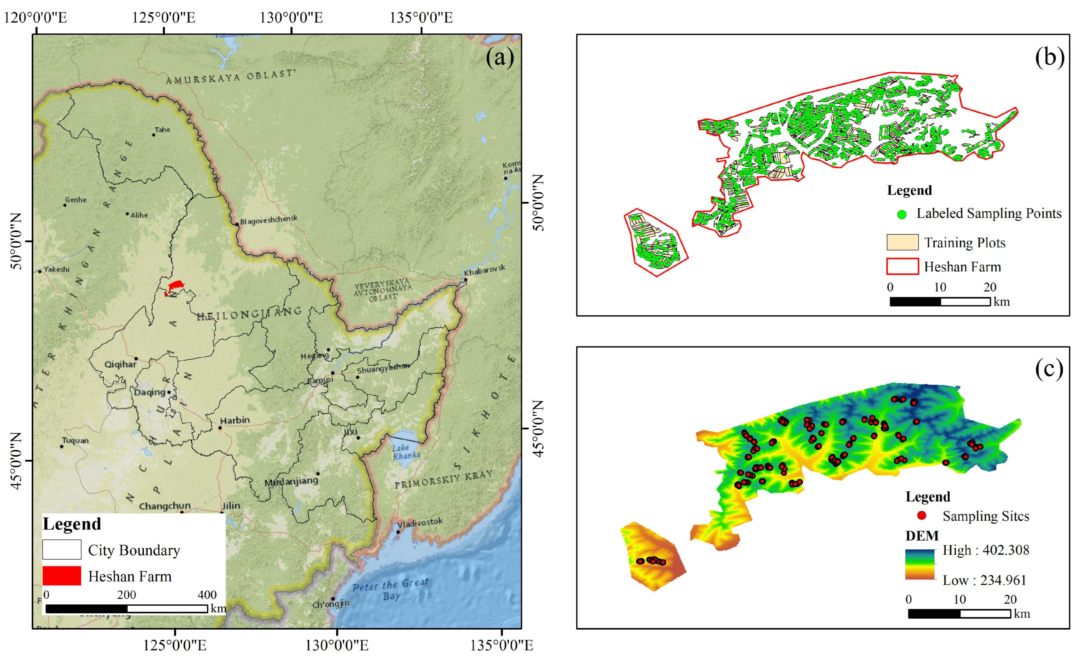
2.1. Study Area

The study area is located in Heshan Farm, Heihe City, Heilongjiang Province, China. It has geographic coordinates ranging from 48°43′N to 49°03′N and 124°56′E to 126°21′E and is situated in the transitional zone from the Lesser Khingan Range to the Songnen Plain. The region’s topography is complex and diverse, primarily characterized by long, gentle slopes, with an effectively cultivated area of approximately 308.8 square kilometers. The soil types in Heshan Farm are predominantly fertile black soil, rich in resources. The climate, classified as cold temperate continental, is marked by windy springs, a short and hot summer, rapid cooling in autumn, and a long, cold winter. The extreme highest temperature reaches around 36 °C, while the extreme lowest temperature can drop to about −38 °C. The annual temperature above 10 °C ranges from 2000 to 2300 degrees days, and the frost-free period is 115 to 120 days. The annual precipitation ranges from 500 to 600 mm, mainly concentrated in July and August. Land use is primarily agricultural, with the main crops being soybeans and corn, making it a typical dryland farming area. Heshan Farm, with its fertile soil suitable for agriculture, is one of the important agricultural bases in Heilongjiang Province. The specific location of the study area is shown in Figure 1.

2.2. Data Acquisition and Processing

2.2.1. Remote Sensing Image Data Acquisition and Pre-Processing

The Sentinel-2 series is a key part of the Copernicus Program, operated by the European Space Agency for environmental monitoring. This series includes two satellites, Sentinel-2A and Sentinel-2B, which both orbit at an altitude of 786 km. Individually, each satellite has a revisit period of 10 days, but when functioning in tandem, this interval is reduced to 5 days. Equipped with a multispectral imager, Sentinel-2 features 13 spectral channels that span from visible light to near-infrared (NIR) and short-wave infrared (SWIR) regions. The Sentinel-2 satellite data used in this study provide ground resolutions from 10 m to 60 m. The Sentinel-2 Level-2A (L2A) products were used in this research. They were obtained from the Google Earth Engine platform (https://earthengine.google.com/; accessed on 5 October 2024). Through this platform, we selected and downloaded seven L2A products, which encompassed the timeframe from April to October 2023. These products were chosen for their minimal cloud cover—less than 5%—and absence of snow. L2A products offer surface reflectance data that are both geometrically and atmospherically corrected. They encompass several spectral bands, with Bands 1 (aerosol), 9 (water vapor), and 10 (cirrus) dedicated to atmospheric correction and cloud detection [37]. Given their sensitivity to atmospheric conditions over surface properties, these bands were excluded from our study. Our research focused on bands that more accurately represent surface characteristics relevant to our objectives. Bands B2, B3, B4, B5, B6, B7, B8, B8A, B11, and B12 were predominantly utilized (Table 1). To ensure data consistency, we resampled the resolution of Bands B5, B6, B7, B8A, B11, and B12 from 20 m to 10 m and carried out subsequent data processing.

2.2.2. Sample Labeling

In remote sensing image recognition, the accuracy and reliability of the results depend largely on the quality and quantity of the sample data used, and high-quality and sufficient sample data are essential for constructing a high-performance recognition model. Topsoil loss is particularly evident during the bare soil period in April and May [38], but since some of the arable land is still covered with straw in April, the optimal window for observation is May. To minimize the interference from other terrestrial features and the spectral information of different crops, and to address the potential imbalance of sample categories, we proportionally selected the number of labeled samples based on the corresponding cropland area. A total of 810 farmland areas were selected in the study area. With the help of Google Earth’s high-resolution images, visual discrimination and labeling were carried out within the farmland, supplementary investigations were carried out in doubtful places, and the labeled data were corrected according to the spatial differences in the soil obtained, in order to improve the accuracy and applicability of the data. A total of 1143 samples were labeled, and the training and test samples were randomly assigned in the code according to the division ratio of 7:3. Details of the selected plots are shown in Figure 1b.

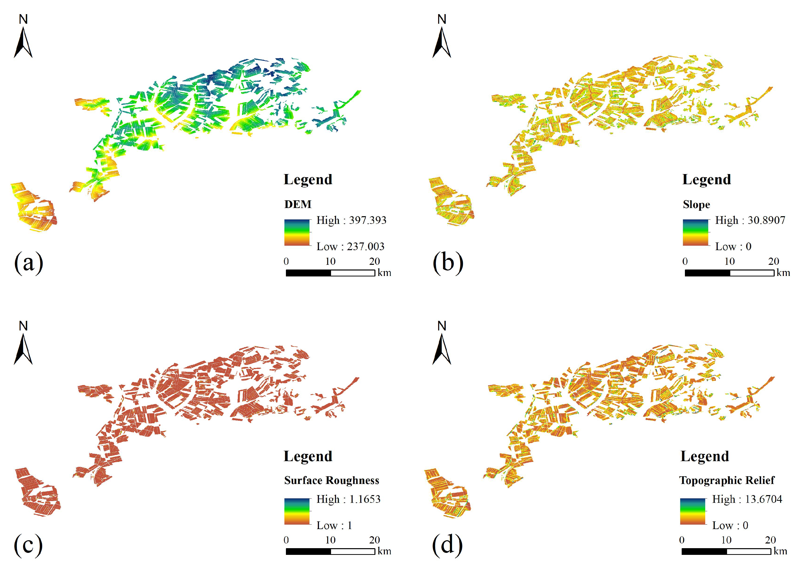
2.2.3. Topographic Data Acquisition and Processing

The topographic data are derived from the Digital Elevation Model (DEM) provided by 91 Wei Tu Assistant (https://www.91weitu.com/) (accessed on 5 October 2024), with a spatial resolution of 6 m. Resampled to 10 m using ArcMap software (version 10.6), we extracted parameters such as slope, roughness, and relief. Slope refers to the steepness of the terrain, defined as the ratio of the vertical height to the horizontal distance of a slope face, which is the tangent of the slope angle [39]. Topographic relief is the difference between the maximum and minimum elevations within an area, serving as a quantitative indicator of landform morphology, reflecting the altitude and surface fragmentation of the region [40]. Surface roughness, from a geomorphological perspective, is defined by the degree of unevenness of the ground, also known as micro-topography [41]. The extraction of topographic factors is shown in Figure 2.

2.2.4. Collection and Processing of Soil Sample Data

Since soil texture does not change significantly over a short timescale of 1 to 10 years [2], field collection of soil samples and acquisition of imagery data can be conducted separately over time. The soil samples used in this study were collected in April 2023, with the soil surface free of vegetation cover and crop residues. Combining remote sensing imagery with field investigations, representative sampling points were selected within the cultivated land of the study area for sampling. A total of 152 sampling points were selected, with a sampling depth of 20 cm. High-precision RTK (Real-Time Kinematic) instruments were used to record and number the exact geographic locations of the sampling points, as shown in Figure 1c. The collected soil samples were stored in cloth soil bags and then brought indoors for soil sample mass measurement, air-drying, grinding, and sieving before soil parameter determination. Multiple methods were used to measure different components of the soil. Specifically, the calcium chloride solution method was used for soil pH; the potassium dichromate volumetric method was for measuring soil organic matter (SOM); the Kjeldahl method was employed to assess total nitrogen (TN); the alkaline hydrolysis diffusion method was used to determine available nitrogen (AN); the Olsen method was used to measure available phosphorus (AP); and flame photometry was used to assess available potassium (AK).

2.3. Spectral Feature Index Construction

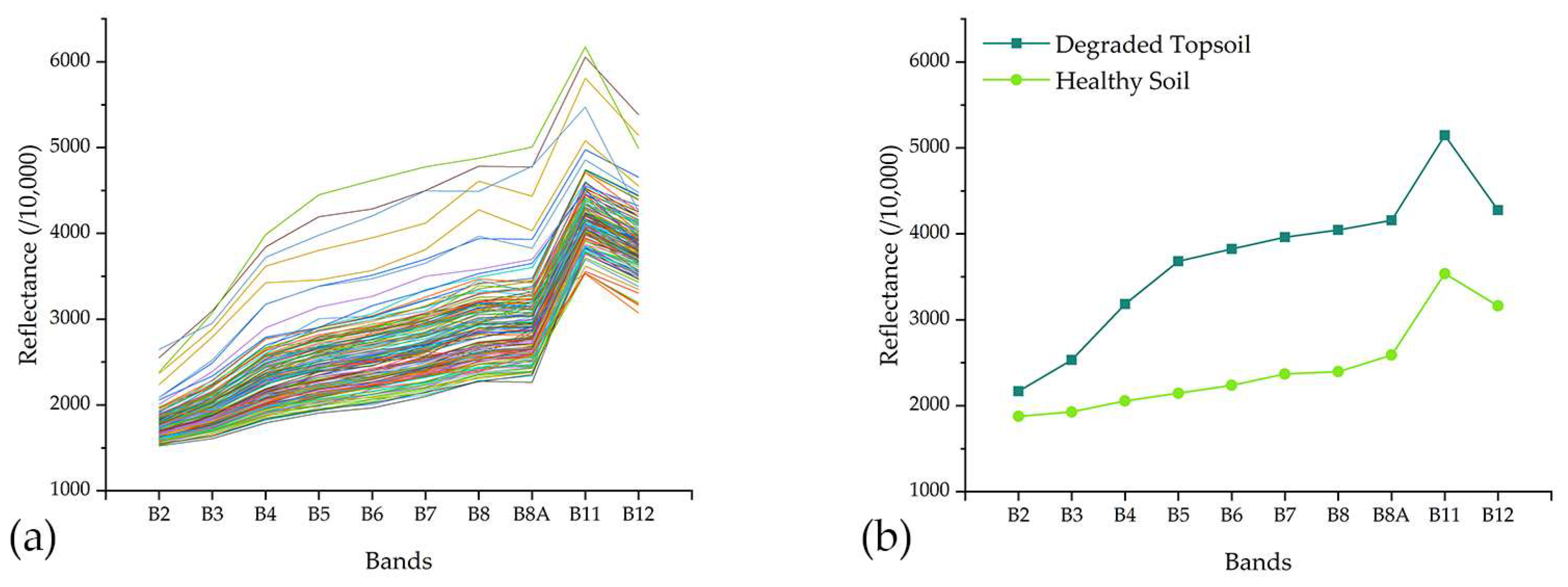
2.3.1. Spectral Analysis

In remote-sensing image analysis, classification and identification based on the spectral characteristics of the features is a more commonly used technical means at present. By utilizing the spectral curve information of the features, the remote-sensing image can be effectively classified and assessed in terms of accuracy [42]. The spectral information of the 152 soil samples in the study area was extracted and the spectral reflectance curves were plotted to compare their differences. Figure 3a displays the spectral curves of all samples, while Figure 3b shows the average reflectance curves of the soil-sample points. The spectral characteristics of surface-degraded soil and healthy soil exhibit distinct differences across various bands. Moreover, the lower the SOM content, the higher the soil spectral reflectance [43]. This suggests that the loss of the topsoil layer not only changes the physical structure of the soil, but also has a significant impact on its optical properties. At the same time, band B11 is more sensitive to soil moisture content, which may also contribute to the reflectivity peaks [44]. The topsoil layer is usually well structured, including aggregates and pores, and these structures facilitate water infiltration and storage. With the loss of the topsoil layer, the underlying soil tends to be less structured and less porous, affecting water infiltration and retention [45]. The index enhances the ability to distinguish between different features; when the spectral reflectance curves of different features trend similarly, it may be difficult to distinguish them by directly comparing reflectance values. By combining information from multiple bands, the index can amplify these small differences, thus identifying different feature types more effectively.

2.3.2. Spectral Index Extraction

Feature extraction is a key step in remote sensing classification, which helps the classifier to better recognize and distinguish different surface cover types by extracting meaningful information from the original remote sensing data [46]. Combining multiple variable features can effectively improve the accuracy of remote sensing classification. This method not only enhances the discriminative power of the classifier but also reduces the misclassification issues that may arise from relying on a single feature [47]. Spectral indices are quantitative indicators used in remote sensing data analysis to enhance the contrast of specific land features or extract specific land feature information [48]. In remote sensing image classification, spectral indices can act as feature variables, assisting computers in better recognizing and distinguishing different types of land features. By combining different spectral observation channels based on the spectral characteristics of land features, it is possible to quantitatively analyze and monitor surface cover types, growth conditions, vegetation content, soil properties, and other information. Therefore, to reflect the spectral characteristics of topsoil loss, further analysis of the correlation between spectral indices and soil spatial heterogeneity is required. We selected vegetation indices that show significant changes in organic matter content; brightness indices that are sensitive to soil texture and can reflect the physical properties of soil structure, mineral composition, and particle size; bare soil indices that can identify and quantify exposed soil areas on the surface; and moisture indices that can monitor changes in soil moisture content [49,50,51]. The introduction of additional non-vegetation indices can further assist in distinguishing and contrasting, including NDVI [52], EVI [53], RVI [54], BI [55], MSI [56], LSWI [57], NDSI [58], and BSI [59]. These indices are considered independent spectral bands, participating in classification tasks to assist in the calibration of land cover classification as feature bands. Upon extensive evaluation, the indices EVI, RVI, MSI, and BSI demonstrated suboptimal performance in various experimental trials, leading to their exclusion from further analysis. Ultimately, a total of four indices were involved in the classification. The formulas for these indices are shown in Table 2.

2.4. Models and Optimization

All machine learning algorithms were implemented using Python version 3.9.18, with the scikit-learn library for machine learning and the sko library for implementing the PSO algorithm. The PSO algorithm is employed to optimize the hyperparameters of RF and SVM models, aiming to maximize their OA on the test dataset. In the PSO-RF optimization, the objective function takes max_depth (maximum depth of the decision trees, range [1, 20]) and n_estimators (number of decision trees, range [1, 100]) as inputs. The former parameter, max_depth, controls the model’s complexity, while n_estimators affects its stability. In the PSO-SVM optimization, the SVM employs a radial basis function (RBF) kernel, with the objective function taking C (penalty coefficient, range [0.01, 1]) and gamma (kernel function parameter, range [0.00000001, 1]) as inputs. C impacts the model’s generalization ability, while gamma determines its nonlinear fitting capacity. The optimization process involves initializing a swarm of particles, each representing a candidate parameter combination. The particles’ velocities and positions are iteratively updated based on their individual and global performance, as evaluated by the objective function, to identify the optimal parameter configuration that maximizes the OA. The optimal parameters obtained through PSO are then used to train the RF and SVM models, achieving their respective best performances.

2.4.1. Random Forest

The RF is an ensemble learning algorithm proposed by Breiman in 2001. It utilizes the Classification and Regression Tree (CART) as the base model and constructs multiple decision trees. The final prediction outcome is derived from the voting results of these trees [60]. RF leverages bootstrapping and random feature selection to build multiple decision trees, enhancing model diversity and predictive accuracy. Random Forest exhibits strong robustness, effectively handling noisy data and outliers. They are capable of managing a large number of input variables without the need for feature selection or dimensionality reduction during model construction. By assessing the importance of each input feature, Random Forest can identify key features that contribute to distinguishing soil differences. Moreover, RF has a good ability to capture complex patterns and nonlinear relationships in remote sensing data and is less sensitive to overfitting. It can maintain high classification performance even with a multitude of noisy variables or redundant features [34,61].

2.4.2. Support Vector Machines

SVM is an advanced classification model proposed by Cortes and Vapnik et al. in 1995 based on the principle of structural risk minimization [62]. The core idea of the SVM model is to use nonlinear mapping techniques to transform nonlinearly separable data into a high-dimensional feature space and to find the optimal classification hyperplane within that space. As a general linear classifier, SVM performs binary classification on data through supervised learning. It selects an appropriate kernel function to construct a classification hyperplane in the determined feature space and uses a regularization factor to balance the maximization of the margin and the minimization of training errors, thereby achieving efficient binary classification of samples. SVM addresses the curse of dimensionality and nonlinear separability through kernel functions, enabling it to effectively handle complex feature spaces in remote sensing data, including morphological, textural, and color features. The kernel trick of SVM is particularly effective in dealing with nonlinear data; it maps the original data to a higher-dimensional feature space to find a linearly separating hyperplane, which is especially important for remote sensing image classification where the actual boundaries between land cover classes may be nonlinear [63,64].

2.4.3. Particle Swarm Optimization

PSO is a swarm intelligence-based optimization algorithm proposed by Eberhart and Kennedy in 1995 [65]. Inspired by the foraging behavior of bird flocks, it simulates the social behaviors of biological groups, such as birds or fish schools, to solve problems. In each iteration of the PSO algorithm, each particle adjusts its velocity and position based on its individual best and the swarm’s global best, exploring new potential solutions. In this way, the swarm as a whole gradually converges towards the global optimal solution. The basic formulas of the Particle Swarm algorithm are shown as Equations (1) and (2).
v i t + 1 = ω v i t + c 1 r 1 p b e s t i t x i t + c 2 r 2 g b e s t t x i t
x i t + 1 = x i t + v i t + 1
Equation (1) v i t + 1 represents the velocity of particle i at iteration; ω is the inertia weight; c 1 and c 2 are learning factors, typically ranging from 1 to 2, which control the convergence of the particle towards its individual best and the global best, respectively; r 1 and r 2 are random numbers between [0, 1], used to introduce randomness into the algorithm; p b e s t i t is the individual best position of particle i at iteration t ; g b e s t t is the global best position of the swarm at iteration t . The position of particle i at iteration t is denoted as x i t . Equation (2) represents the position of particle i at iteration t + 1 . By optimizing RF and SVM with PSO, it is possible to improve the classification performance, computational efficiency, and robustness of the models to some extent, and to reduce the complexity of manual parameter tuning, thus promoting the automation and efficiency of the model development process. However, the effectiveness of PSO may depend on the specific application scenarios and characteristics of the dataset, so its advantages should be assessed under certain conditions.

2.5. Classification Results and Accuracy Assessment

In this study, to comprehensively evaluate the extraction accuracy and performance of the models, we employed a set of comprehensive metrics, including overall accuracy (OA) and the Kappa coefficient. These metrics assess classification performance from different perspectives. OA, as an intuitive evaluation metric, quantifies the proportion of samples that are correctly classified out of the total number of samples. However, when dealing with datasets that have uneven class distributions, relying solely on OA can lead to misleading results. To address this issue, the Kappa coefficient is introduced as a statistical measure to assess the consistency of classifications. The Kappa coefficient takes into account not only the classifier’s prediction results but also the level of agreement due to random chance, thus correcting for the agreement that occurs by chance. Therefore, when dealing with datasets with class imbalance, the Kappa coefficient provides more informative insights than OA [66]. The specific calculation formulas are shown as Equations (3) and (4).
O A = i = 1 n x i i N
K a p p a = P 0 P e 1 P e
In Equation (3), x i i represents the number of samples correctly classified in the i -th class, N is the total number of pixels, and n is the total number of classes. In Equation (4), P 0 represents the actual observed agreement, which is the OA; P e represents the expected agreement, which is the probability of agreement, assuming that the classification is conducted randomly.

2.6. Technological Processes

The research is divided into three parts, as shown in Figure 4, and illustrated below:
(1)
Data Acquisition and Preprocessing: Collect Sentinel-2 satellite imagery and DEM data. Preprocess the collected data to obtain band data and terrain data for the study area. Combine field survey data and visual interpretation to create a labeled dataset for model training. Analyze the reflectance characteristics of ground objects and extract key spectral indices;
(2)
Extraction Scheme Design and Model Construction: Utilize multi-source remote sensing data to design four different land cover extraction schemes. Develop remote sensing monitoring models based on SVM and RF algorithms. Apply the PSO algorithm to optimize the models and enhance their performance;
(3)
Accuracy Assessment and Result Analysis: Evaluate the impact of different features on model performance and analyze the importance of features. Compare the extraction effects and accuracy of the four schemes and different models to determine the optimal extraction scheme and model. Use the extraction results from the optimal model to explore the spatial distribution pattern of topsoil degradation areas and analyze its potential impact on crop growth.

3. Results

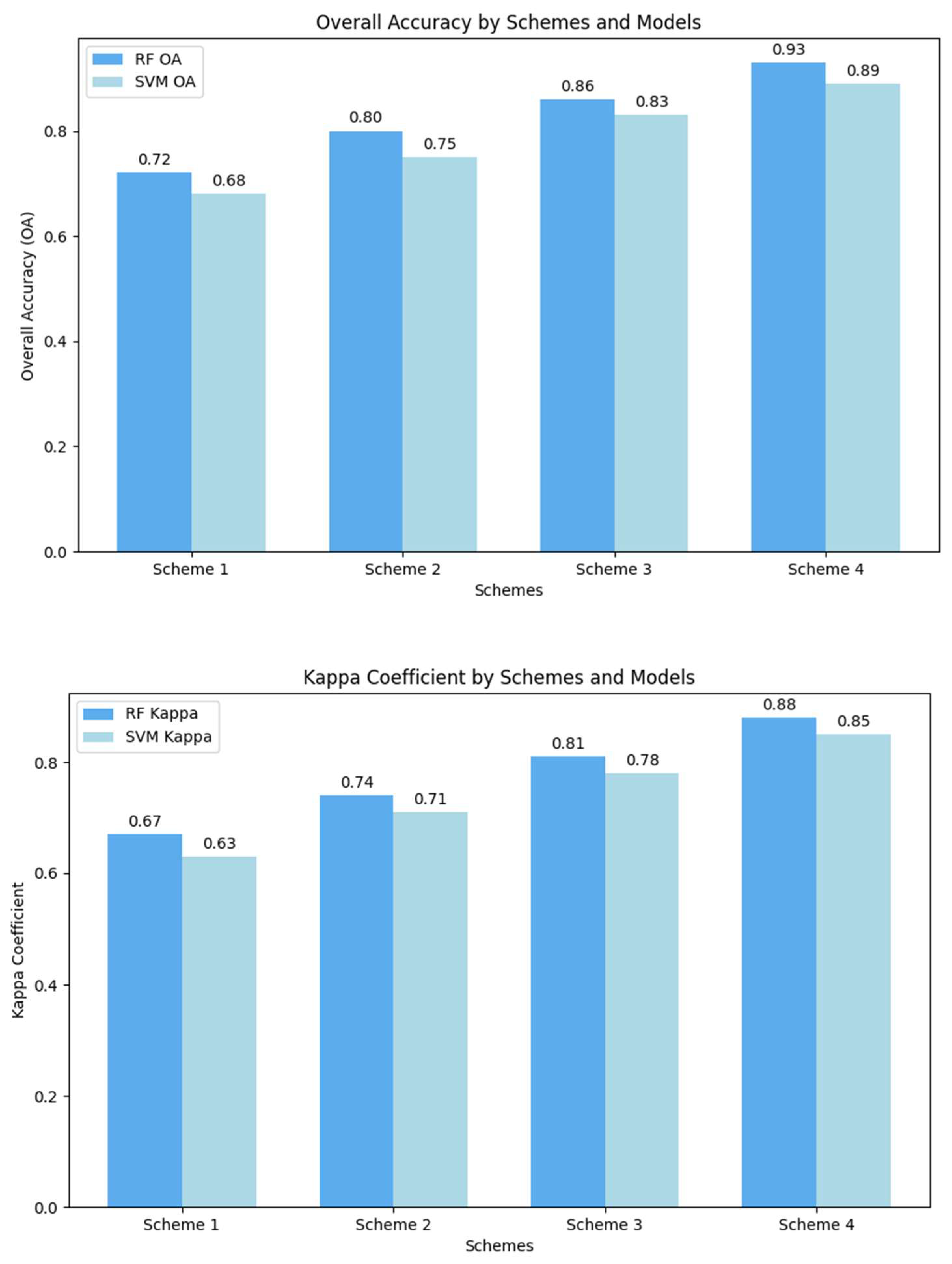
3.1. Comparative Analysis of Feature Combinations and Classification Accuracy

The aim of this study is to compare four feature combination schemes to evaluate the effectiveness of single-spectrum versus multi-source features in extracting TLA. As depicted in Figure 5 and Figure 6, Scheme 1, which relies solely on spectral information, struggles to accurately identify TLA. The RF and SVM models achieve OA of 0.72 and 0.68, respectively, with Kappa coefficients of 0.67 and 0.63. These results indicate low extraction accuracy, unclear boundaries, and significant misclassification. In contrast, Scheme 2 and Scheme 3 enhance the identification of TLA through different approaches. Scheme 2 incorporates topographic features, while Scheme 3 integrates spectral indices. The introduction of these features enhances the accuracy of identifying TLA. Scheme 3 slightly outperforms Scheme 2, with RF and SVM models achieving OA of 0.86 and 0.83, respectively, and Kappa coefficients of 0.81 and 0.78. Scheme 4 provides the highest classification accuracy and best extraction performance. The RF model achieves an OA of 0.93 and a Kappa coefficient of 0.88, while the SVM model reaches an OA of 0.89 with a Kappa coefficient of 0.85. This demonstrates that integrating topographic features improves classification accuracy, especially in hilly and undulating areas where topographic changes affect object classification. However, spectral indices play an even more crucial role. They not only enhance the spectral characteristics of specific objects but also reduce interference and increase object differentiation.
In conclusion, Scheme 4, which integrates spectral features, topographic features, and spectral indices, achieves the highest accuracy in topsoil loss extraction. It improves contour recognition and significantly reduces background noise. A comparison of all four schemes confirms that Scheme 4, with its combination of multi-source features, outperforms the others. Notably, the inclusion of the Particle Swarm Optimization (PSO) algorithm further boosts the accuracy of both the RF and SVM models in extracting topsoil loss (Table 3). The PSO-RF model achieves an OA of 0.97 with a Kappa coefficient of 0.94, while the PSO-SVM model reaches an OA of 0.94 with a Kappa coefficient of 0.90. The PSO-RF model using Scheme 4 improves OA by 34.72% and Kappa by 38.81%, compared to the RF model in Scheme 1; the PSO-SVM model improves OA by 38.24% and Kappa by 42.86%, compared to the SVM model in Scheme 1. By integrating the PSO-RF model with Scheme 4, which employs multi-source feature fusion, we have achieved the best extraction results. This approach not only optimizes the extraction effect but also yields the highest overall accuracy (OA) and Kappa coefficient among all tested schemes, indicating superior classification performance and reliability.

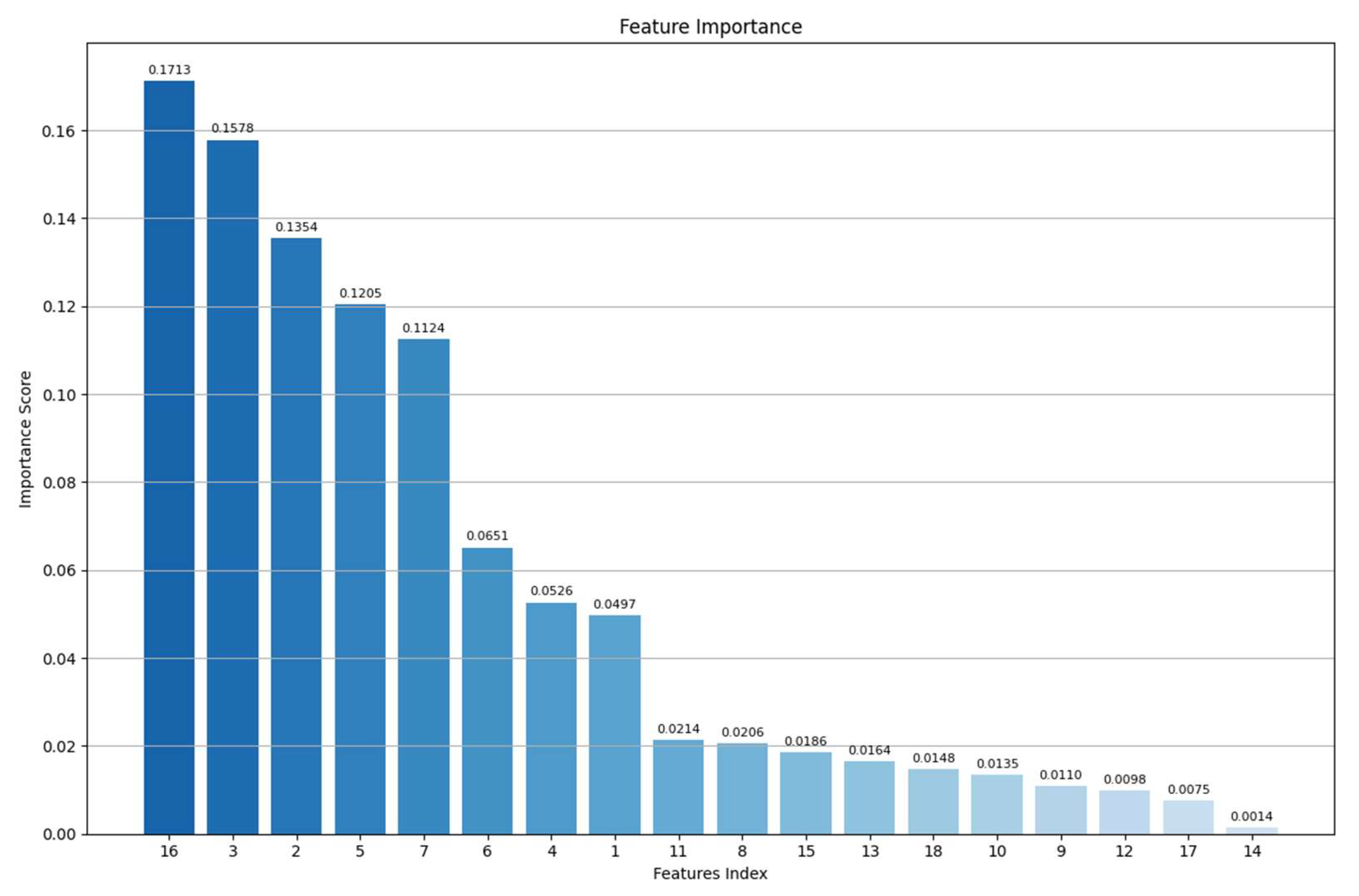
3.2. Feature Importance Analysis of Multi-Source Data

In this study, utilizing multi-source remote sensing data, we extracted 18 effective features (Table 4). The assessment of feature importance through the PSO-RF model indicates that the BI significantly identifies topsoil-layer depletion. Specifically, the importance score of BI is 0.1713 (Figure 7), which is the highest among all features, suggesting its crucial role in the model for predicting TLA. Bands 4, 3, 6, and 8 follow closely in importance. These bands cover the visible to near-infrared spectrum, which is crucial for capturing soil, vegetation conditions, and surface structure information. These data are closely related to the assessment of topsoil loss. Furthermore, elevation, as a key topographic factor, plays a significant role. It highlights the close relationship between topographic variations and processes such as water erosion and sedimentation, which is also important for identifying topsoil-loss areas. Slope, relief, and roughness rank lower in feature importance. This is likely because they are all derived from elevation data. The slope indicates the steepness based on elevation change, relief shows the elevation difference, and roughness reflects the micro-scale elevation variability. Since they mainly present elevation-related information without adding much new content, their predictive power in the model is limited. Although some indices have low individual importance scores, they may provide supplementary information that other features cannot capture. For instance, when combined with elevation data and spectral bands, slope information can contribute to a more comprehensive understanding of the terrain’s influence on topsoil loss. In areas with a specific slope gradient and certain spectral characteristics indicating vulnerable soil conditions, the combined effect can more accurately predict topsoil loss compared to using elevation or spectral bands alone. Relief and roughness, when interacting with other features, can also offer insights into micro-topography, which affects surface runoff and soil detachment processes. Considering the interaction effects between features during model construction and feature selection is crucial. It helps us understand the data structure more comprehensively and enhances model performance. The importance ranking of features reveals the key role of spectral information and topographic conditions in the identification of TLA. This provides a scientific basis for using remote sensing technology to monitor and assess topsoil loss and emphasizes the importance of multi-source data fusion in environmental monitoring.

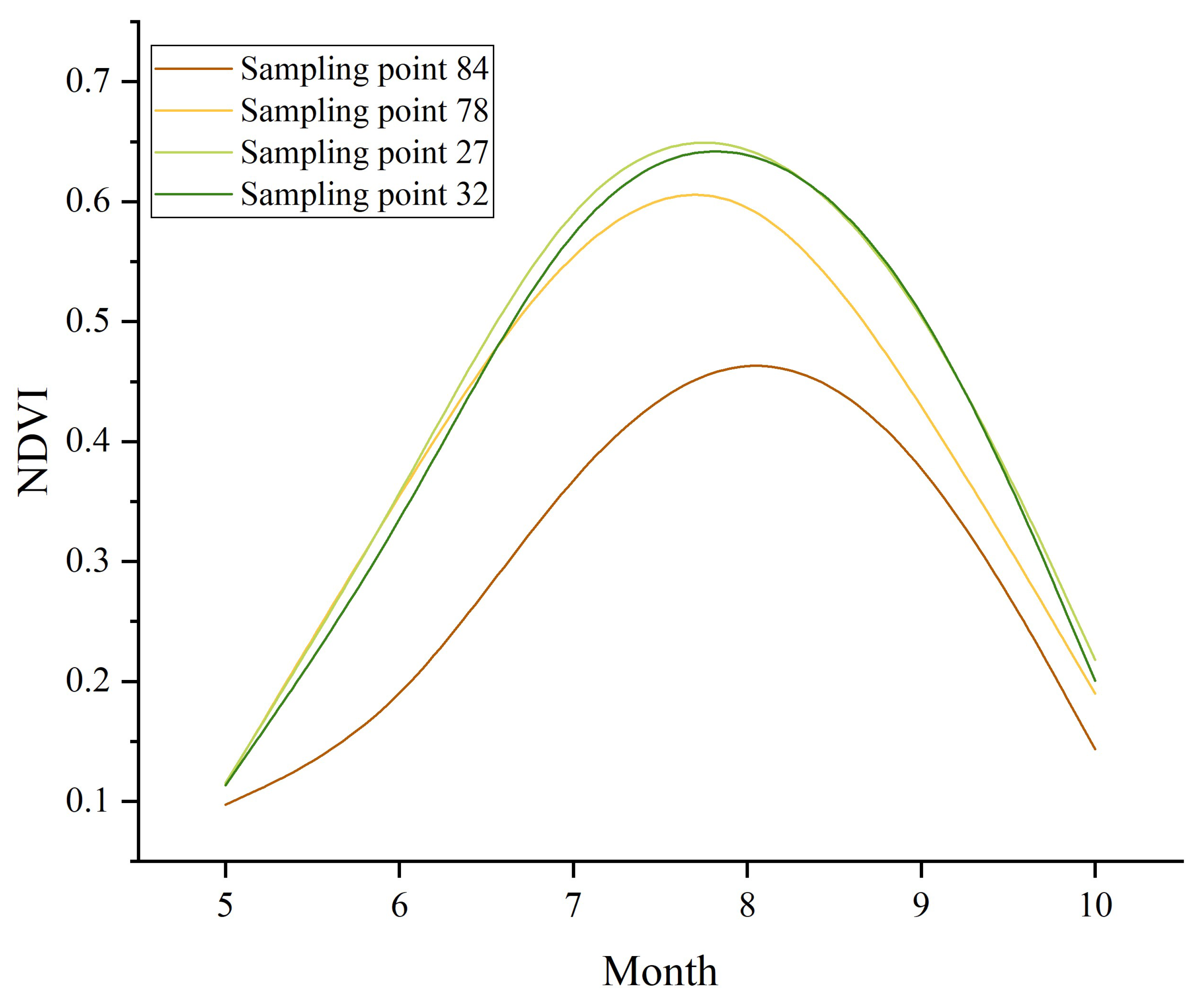
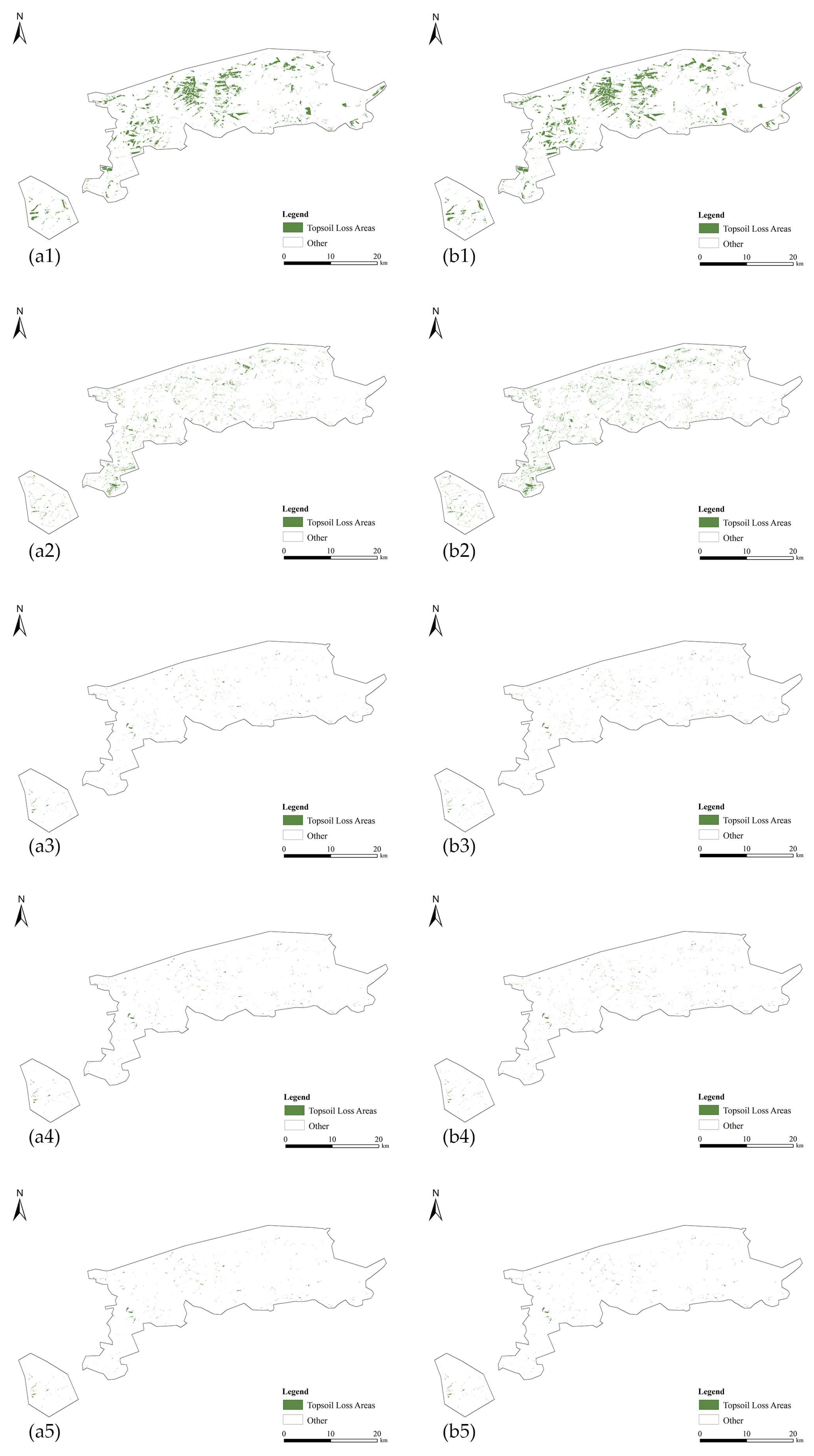
3.3. Spatial Distribution of TLA and Their Impact

The spatial distribution of TLA in Heshan Farm is depicted in Figure 8. The overall topography of Heshan Farm slopes higher in the northeast and lower in the southwest, with the western and southwestern areas being lower and more depressed, while the eastern and northern areas are higher with complex surface undulations, primarily consisting of hills and slopes. Using the extraction results from Scheme 4 and the PSO-RF model as an example, the TLA in Heshan Farm is mainly concentrated in the central and southwestern parts of the farm, where the arable land is more intensive. The TLA appears concentrated but fragmented, rather than continuous large patches. The eastern and northeastern regions have less TLA, with diverse terrain, many hills, and steep slopes, lacking the objective conditions for large-scale crop cultivation. At the same time, these areas have relatively rich vegetation cover, which effectively reduces the risk of soil erosion through the consolidation of soil by plant roots, thereby reducing the incidence of TLA. This complex terrain increases the difficulty of TLA extraction and also poses a greater challenge for remediation efforts.
Figure 8(a1,b1–b3) show the local magnified views, clearly demonstrating that there is partial overlap between the TLA and areas with lower NDVI during the crop-growth period. The NDVI in TLA areas is generally lower than that in surrounding normal soil areas and has a significant impact on the entire growth cycle of crops. The vegetation-growth condition in this area is poor, which is significantly correlated with soil quality. The soil structure in TLA areas is severely damaged, affecting the soil’s permeability and aeration. Meanwhile, the soil fertility in TLA areas has significantly decreased, lacking necessary organic matter and readily available nutrients such as nitrogen, phosphorus, and potassium, which are key nutrients for crop growth. The decline in soil fertility directly affects the nutrient absorption and growth development of crops. Furthermore, organic matter in the soil is a key factor in water retention, and due to the reduction in organic matter, the soil’s water-holding capacity decreases, making it difficult for crops to obtain sufficient water during their growth process, thereby hindering crop growth (Appendix A Figure A1 and Figure A2, Table A1). Improving soil quality and restoring the ecological balance have therefore become key measures for increasing crop yields and achieving sustainable agricultural development in the region.

4. Discussion

4.1. Analysis of the Necessity of Integrating Multi-Source Features

This study integrated multi-source remote sensing data to extract 18 features encompassing spectral, topographic, and index dimensions, providing a more comprehensive revelation of the complex information in TLA and significantly enhancing the accuracy and reliability of geospatial analysis. After comparing different extraction schemes, subsequent experiments adopted the extraction method from Scheme 4, which combines spectral features, topographic features, and various indices, leading to a marked improvement in evaluation indicators, such as OA and Kappa coefficients, compared to other schemes. Topographic features, as descriptors of surface undulations and terrain structure, are crucial for understanding the distribution and causes of TLA [19]. Slope directly impacts natural processes such as soil erosion and water-soil loss. This direct effect indirectly determines the formation and distribution of TLA. The undulation and relative elevation differences in the terrain can reflect the intensity of surface erosion and deposition. This provides important clues for revealing the formation mechanisms and evolutionary processes of TLA [67]. Through the analysis of topographic features, a deeper understanding of the impact of these environmental factors on TLA can be achieved, providing a scientific basis for subsequent geospatial analysis and decision-making. Additionally, the application of indices has played a significant role in the extraction of TLA. Indices, which are comprehensive indicators derived from mathematical operations on multiple remote sensing parameters, can effectively assess surface conditions or specific phenomena [68]. Vegetation indices and moisture indices are helpful in identifying vegetation cover and soil-moisture conditions, while brightness indices and bare soil indices assist in recognizing surface exposure and changes in reflectance [55]. In this research, an innovative approach is adopted to integrate multi-source remote sensing data to extract 18 features. These features comprehensively capture the intricate information of TLA from multiple dimensions, thereby filling certain voids in the domain of comprehensively leveraging multi-source data for TLA analysis. The proposed multi-source feature fusion methodology not only significantly enhances the accuracy and reliability of TLA extraction but also offers novel perspectives and methodological insights for other geospatial analysis tasks. This advancement is conducive to propelling the application and development of geospatial information science in the analysis of complex environmental scenarios. The developed PSO-RF model has demonstrated remarkable performance in identifying TLA. By optimizing the hyperparameters of the RF model through the PSO algorithm, the model’s performance has been effectively elevated. This achievement furnishes a viable optimization strategy for addressing other analogous classification problems, showcases the potential of the PSO algorithm in enhancing the performance of machine learning models, and facilitates the integration and application of optimization algorithms and machine learning models within the realm of geospatial analysis.

4.2. Uncertainty Analysis of Extraction Results

Relying solely on spectral features to extract TLA presents significant challenges, primarily due to the instability of spectral characteristics, the phenomenon of different objects with the same spectrum, and the limitations of extraction algorithms. Spectral features can be influenced by various environmental factors such as soil moisture, vegetation cover, and lighting conditions, leading to unstable manifestations in remote sensing imagery. Additionally, factors like image resolution, the complexity of surface covers, and the inherent limitations of extraction algorithms can also affect the extraction results, increasing the uncertainty of the outcomes. High-resolution imagery can more clearly display surface features, such as soil morphology, color, and structure. In contrast, medium and low-resolution imagery may not provide sufficient detail to accurately distinguish the subtle spatial heterogeneities within fields, leading to mixed pixels. A single pixel might contain information from multiple land cover types, and the spectral information of that pixel is an average of these different types, rather than an exact representation of a single land cover type. Furthermore, the boundaries of some land covers are often not distinct, and the types in marginal areas may be misclassified, making the patches in the spatial distribution map appear more fragmented and disjointed. Each pixel in medium and low-resolution imagery represents a larger ground area, which can result in more uncertain patches in the extraction results. Field surveys have revealed that some fields contain linear erosion gullies, which, despite topsoil loss, are less than 2 m in scale and may be completely overlooked or mixed with other land covers in Sentinel-2 satellite imagery, making them indistinguishable as separate features.

4.3. Limitations and Future Prospects

The PSO-RF model developed in this study has achieved promising results in identifying TLA. However, the research has certain limitations. Although we extracted various features to enhance the accuracy of TLA extraction, texture features, which can detail the surface structure and arrangement of objects in an image, were not fully incorporated. Texture features are instrumental in revealing the nuances of terrain, especially in capturing micro-topographical variations that are typically difficult to discern with conventional methods. For example, fine-scale roughness or smoothness, as captured by texture features, can indicate regions of soil deposition or erosion. Rough textures, typically indicative of surface irregularities, may suggest areas where the soil has been disturbed due to dynamic processes such as water runoff or wind action—key factors in the formation of TLA. Additionally, the varying spatial resolutions of different satellite sensors can impact the accuracy of classification results; high-resolution imagery, containing more pixels and information, can present more image features and details, thereby more comprehensively describing TLA and improving classification accuracy. While this may increase model complexity, the potential for enhancing classification performance is significant.
Machine learning constructs models by adjusting weights, while deep learning, particularly convolutional neural networks (CNNs), has demonstrated strong performance in remote sensing image classification by automatically extracting high-level features and significantly improving classification accuracy. Traditional machine learning methods face limitations such as complex feature engineering, limited generalization capabilities, and high computational resource demands when dealing with high-dimensional remote sensing data. These methods require manual feature design, are prone to overfitting, and their computational costs rise with increased data volume. Future research will continue to explore the application of deep learning in TLA extraction, aiming to further enhance extraction effects and classification accuracy. Deep learning can automatically learn the most discriminative features, capture multi-scale information, adapt to complex land cover changes, and improve model robustness. However, deep learning has its drawbacks. It has limited interpretability, making it difficult to understand how predictions are made. Additionally, it requires a large amount of high-quality data for training, which is time-consuming and costly to collect. Moreover, it demands substantial computational resources, hindering its widespread use. Given these challenges, integrating traditional machine learning with deep learning is a promising solution. Traditional algorithms like decision trees are highly interpretable, while deep learning models excel at automatic complex feature extraction. Future studies can build hybrid models for TLA identification and sustainable agricultural development. For example, they can use decision trees for feature selection first to reduce data dimensionality and then feed the processed data into a neural network for further pattern extraction. Two key points should be noted when developing such models. First, ensure the compatibility of different algorithms, as their data requirements may vary. Second, comprehensively evaluate the model’s performance, considering both identification accuracy and interpretability using relevant metrics. This integrated approach holds the potential to advance our understanding and management of agricultural ecosystems.

5. Conclusions

Timely and accurate identification of the distribution of TLA is fundamental to sustainable land management and ecological conservation. This aids in the rational planning of land use, implementation of targeted soil and water conservation measures, enhancement of soil fertility, and ensuring the stability and continuity of agricultural production. It also plays a significant role in preventing natural disasters and maintaining ecological balance. This study successfully developed an effective method for TLA extraction using multi-source remote sensing data and a PSO-RF model. The main conclusions of this study are as follows: (1) Scheme 4, which combines spectral features, topographic features, and index bands, demonstrated the highest accuracy in extracting TLA areas. The extraction effects of various methods are ranked as follows: spectral + topographic + index > spectral + index > spectral + topographic > spectral only. (2) The BI is a key feature for identifying TLA, featuring an importance weight of 0.1713. (3) Regardless of the extraction scheme employed, the Random Forest (RF) model outperforms the Support Vector Machine (SVM) model. (4) The PSO-RF model outperformed the PSO-SVM model, achieving an overall accuracy of 0.97 and a Kappa coefficient of 0.94, thereby demonstrating superior performance among all the models tested. (5) During the growing season, the NDVI of the topsoil loss-affected areas was significantly lower than that of the surrounding non-degraded areas, indicating severe inhibition of crop growth.

Author Contributions

Author Contributions: Conceptualization, X.Z. and H.L.; data curation, C.Q. and Y.W.; formal analysis, C.Q., S.M. and Y.W.; methodology, X.Z., Y.W. and C.Q.; project administration, X.Z. and H.L.; software, J.L., Z.A. and Y.M.; writing—original draft, X.Z. and C.Q.; writing—review and editing, X.Z. and Y.W. All authors have read and agreed to the published version of the manuscript.

Funding

This research was supported by the National Key R&D Program of China (2024YFD1501100), the National Key R&D Program of China (2021YFD1500100), the Science and Technology Development Plan Project of Jilin Province, China (20240101043JC), and the Jilin Agricultural University Introduction of Talents Project (No.202020010).

Data Availability Statement

Data are subject to privacy restrictions. Please contact the corresponding author.

Acknowledgments

We thank the National Earth System Science Data Center for providing geographic information data.

Conflicts of Interest

The authors declare no conflicts of interest.

Appendix A

Figure A1. Distribution of sampling points at local zoom-in locations; the names of the sampling points are 84, 78, 27, and 32, respectively.
Remotesensing 17 00547 g0a1
Figure A2. NDVI time series curves for localized sampling points.
Remotesensing 17 00547 g0a2
Table A1. Parameters of physical and chemical properties of soil at sampling sites.
Sampling PointpHSOMTNANAPAK
845.240.86545159417.118201978.968421.72589.2326
785.513.0993680291293.14923269.421625.225111.216
275.863.789980681835.146267309.6820.77599.0112
325.784.6199415062025.65445301.93821.85116.884

References

  1. Chen, J.; Chen, J.Z.; Tan, M.Z.; Gong, Z. Soil degradation: A global problem endangering sustainable development. J. Geogr. Sci. 2002, 12, 243–252. [Google Scholar]
  2. Lehmann, J.; Bossio, D.A.; Kögel-Knabner, I.; Rillig, M.C. The concept and future prospects of soil health. Nat. Rev. Earth Environ. 2020, 1, 544–553. [Google Scholar] [CrossRef] [PubMed]
  3. Patzold, S.; Mertens, F.M.; Bornemann, L.; Koleczek, B.; Franke, J.; Feilhauer, H.; Welp, G. Soil heterogeneity at the field scale: A challenge for precision crop protection. Precis. Agric. 2008, 9, 367–390. [Google Scholar] [CrossRef]
  4. Mulla, D.J.; McBratney, A.B. Soil spatial variability. In Soil Physics Companion; CRC Press: Boca Raton, FL, USA, 2001; pp. 343–373. [Google Scholar]
  5. Reynolds, H.L.; Haubensak, K.A. Soil fertility, heterogeneity, and microbes: Towards an integrated understanding of grassland structure and dynamics. Appl. Veg. Sci. 2009, 12, 33–44. [Google Scholar] [CrossRef]
  6. Pacheco, F.A.L.; Fernandes, L.F.S.; Junior, R.F.V.; Valera, C.A.; Pissarra, T.C.T. Land degradation: Multiple environmental consequences and routes to neutrality. Curr. Opin. Environ. Sci. Health 2018, 5, 79–86. [Google Scholar] [CrossRef]
  7. Prăvălie, R.; Patriche, C.; Borrelli, P.; Panagos, P.; Roșca, B.; Dumitrașcu, M.; Bandoc, G. Arable lands under the pressure of multiple land degradation processes. A global perspective. Environ. Res. 2021, 194, 110697. [Google Scholar] [CrossRef] [PubMed]
  8. Vågen, T.G.; Winowiecki, L.A. Predicting the spatial distribution and severity of soil erosion in the global tropics using satellite remote sensing. Remote Sens. 2019, 11, 1800. [Google Scholar] [CrossRef] [PubMed]
  9. Wang, H.; Yang, S.; Wang, Y.; Gu, Z.; Xiong, S.; Huang, X.; Sun, M.; Zhang, S.; Guo, L.; Cui, J.; et al. Rates and causes of black soil erosion in Northeast China. Catena 2022, 214, 106250. [Google Scholar] [CrossRef]
  10. Ma, S.; Wang, L.J.; Wang, H.Y.; Zhao, Y.G.; Jiang, J. Impacts of land use/land cover and soil property changes on soil erosion in the black soil region, China. J. Environ. Manag. 2023, 328, 117024. [Google Scholar] [CrossRef]
  11. Sun, Z.; Liu, F.; Wu, H.; Zhang, G.L. Development of a national black soil map of China through machine learning classification. Catena 2024, 240, 107993. [Google Scholar] [CrossRef]
  12. Han, X.; Li, N. Research progress of black soil in Northeast China. Sci. Geogr. Sin. 2018, 38, 1032–1041. [Google Scholar]
  13. Zhao, Z.; Zhang, C.; Wang, H.; Li, F.; Pan, H.; Yang, Q.; Zhang, J. The effects of natural humus material amendment on soil organic matter and integrated fertility in the black soil of Northeast China: Preliminary results. Agronomy 2023, 13, 794. [Google Scholar] [CrossRef]
  14. Liu, B.; Ye, Y.; Li, Z.; Liang, Y.; Zhang, W.; Fu, S.; Yin, S.; Wei, X. The assessment of soil loss by water erosion in China. Int. Soil Water Conserv. Res. 2020, 8, 430–439. [Google Scholar] [CrossRef]
  15. Wang, S.; Liang, X.; Wei, C. Spatial and temporal changes of erosion in the black soil region of Northeast China from 2000 to 2020. Ziyuan Kexue 2023, 45, 951–965. [Google Scholar] [CrossRef]
  16. Liu, J.; Han, X.; Chen, X.; He, R.; Wu, P. Prediction of soil thicknesses in a headwater hillslope with constrained sampling data. Catena 2019, 177, 101–113. [Google Scholar] [CrossRef]
  17. Qi, Z.J.; Zhang, Z.X.; Yang, A.Z. Benefit of soil and water conservation measures on sloped land of black soils. Res. Soil Water Conserv. 2011, 18, 72–75. [Google Scholar]
  18. Li, X.; Shi, Z.; Zhang, Z.; Wang, M.; Wang, M. Dynamic evaluation of cropland degradation risk by combining multi-temporal remote sensing and geographical data in the Black Soil Region of Jilin Province, China. Appl. Geogr. 2023, 154, 102920. [Google Scholar] [CrossRef]
  19. Thaler, E.A.; Larsen, I.J.; Yu, Q. The extent of soil loss across the US Corn Belt. Proc. Natl. Acad. Sci. USA 2021, 118, e1922375118. [Google Scholar] [CrossRef] [PubMed]
  20. Yu, H.; Chen, P.; Sun, Y. Analysis of the coupling and coordination between soil erosion and land use in the Northeastern black soil region of China: A case study of Lishu County. Sci. Rep. 2024, 14, 21955. [Google Scholar] [CrossRef]
  21. Han, X.Z.; Zou, W.X. Research Perspectives and Footprint of Utilization and Protection of Black Soil in Northeast China. Acta Pedol. Sin. 2021, 58, 1341–1358. [Google Scholar]
  22. Cui, J.; Guo, L.; Xiong, S.; Yang, S.; Wang, Y.; Zhang, S.; Sun, H. Soil organic carbon induces a decrease in erodibility of black soil with loess parent materials in Northeast China. Quat. Res. 2024, 120, 83–92. [Google Scholar] [CrossRef]
  23. Li, C.; Fu, B.; Wang, S.; Stringer, L.C.; Wang, Y.; Li, Z.; Zhou, W. Drivers and impacts of changes in China’s drylands. Nat. Rev. Earth Environ. 2021, 2, 858–873. [Google Scholar] [CrossRef]
  24. Shi, Y.; Yang, F.; Long, H.; Rossiter, D.G.; Zhang, A.; Zhang, G. Provenance of soil parent materials in relation to regional environmental changes in the Songnen Plain, Northeast China. Geoderma Reg. 2024, 38, e00848. [Google Scholar] [CrossRef]
  25. Alewell, C.; Borrelli, P.; Meusburger, K.; Panagos, P. Using the USLE: Chances, challenges and limitations of soil erosion modelling. Int. Soil Water Conserv. Res. 2019, 7, 203–225. [Google Scholar] [CrossRef]
  26. Borrelli, P.; Alewell, C.; Alvarez, P.; Anache, J.A.A.; Baartman, J.; Ballabio, C.; Bezak, N.; Biddoccu, M.; Cerdà, A.; Chalise, D.; et al. Soil erosion modelling: A global review and statistical analysis. Sci. Total Environ. 2021, 780, 146494. [Google Scholar] [CrossRef] [PubMed]
  27. Kulyanitsa, A.L.; Rukhovich, D.I.; Koroleva, P.V.; Vilchevskaya, E.V.; Kalinina, N.V. Analysis of the informativity of big satellite precision-farming data processing for correcting large-scale soil maps. Eurasian Soil Sci. 2020, 53, 1709–1725. [Google Scholar] [CrossRef]
  28. Liu, J.; Yang, K.; Tariq, A.; Lu, L.; Soufan, W.; El Sabagh, A. Interaction of climate, topography and soil properties with cropland and crop pattern using remote sensing data and machine learning methods. Egypt. J. Remote Sens. Space Sci. 2023, 26, 415–426. [Google Scholar]
  29. Bag, R.; Mondal, I.; Dehbozorgi, M.; Bank, S.P.; Das, D.N.; Bandyopadhyay, J.; Pham, Q.B.; Al-Quraishi, A.M.; Nguyen, X.C. Modelling and mapping of soil erosion susceptibility using machine learning in a tropical hot sub-humid environment. J. Clean. Prod. 2022, 364, 132428. [Google Scholar] [CrossRef]
  30. Schmid, T.; Rodríguez-Rastrero, M.; Escribano, P.; Palacios-Orueta, A.; Ben-Dor, E.; Plaza, A.; Milewski, R.; Huesca, M.; Bracken, A.; Cicuéndez, V.; et al. Characterization of soil erosion indicators using hyperspectral data from a Mediterranean rainfed cultivated region. IEEE J. Sel. Top. Appl. Earth Obs. Remote Sens. 2015, 9, 845–860. [Google Scholar] [CrossRef]
  31. Žížala, D.; Juřicová, A.; Zádorová, T.; Zelenková, K.; Minařík, R. Mapping soil degradation using remote sensing data and ancillary data: South-East Moravia, Czech Republic. Eur. J. Remote Sens. 2019, 52 (Suppl. S1), 108–122. [Google Scholar] [CrossRef]
  32. Zeng, X.; Guo, X.; Jiang, Y.; Li, W.; Guo, J.; Zhou, Q.; Zou, H. High-accuracy mapping of soil parent material types in hilly areas at the county scale using machine learning algorithms. Remote Sens. 2024, 16, 91. [Google Scholar] [CrossRef]
  33. Daviran, M.; Maghsoudi, A.; Ghezelbash, R. Optimized AI-MPM: Application of PSO for tuning the hyperparameters of SVM and RF algorithms. Comput. Geosci. 2025, 195, 105785. [Google Scholar] [CrossRef]
  34. Sheykhmousa, M.; Mahdianpari, M.; Ghanbari, H.; Mohammadimanesh, F.; Ghamisi, P.; Homayouni, S. Support vector machine versus random forest for remote sensing image classification: A meta-analysis and systematic review. IEEE J. Sel. Top. Appl. Earth Obs. Remote Sens. 2020, 13, 6308–6325. [Google Scholar] [CrossRef]
  35. Akbari, E.; Darvishi Boloorani, A.; Neysani Samany, N.; Hamzeh, S.; Soufizadeh, S.; Pignatti, S. Crop mapping using random forest and particle swarm optimization based on multi-temporal Sentinel-2. Remote Sens. 2020, 12, 1449. [Google Scholar] [CrossRef]
  36. Ramírez-Ochoa, D.D.; Pérez-Domínguez, L.A.; Martínez-Gómez, E.A.; Luviano-Cruz, D. PSO, a swarm intelligence-based evolutionary algorithm as a decision-making strategy: A review. Symmetry 2022, 14, 455. [Google Scholar] [CrossRef]
  37. Gao, B.C.; Goetz, A.; Wiscombe, W.J. Cirrus cloud detection from airborne imaging spectrometer data using the 1.38 μm water vapor band. Geophys. Res. Lett. 1993, 20, 301–304. [Google Scholar] [CrossRef]
  38. Shi, P.; Six, J.; Sila, A.; Vanlauwe, B.; Van Oost, K. Towards spatially continuous mapping of soil organic carbon in croplands using multitemporal Sentinel-2 remote sensing. ISPRS J. Photogramm. Remote Sens. 2022, 193, 187–199. [Google Scholar] [CrossRef]
  39. Olaya, V. Basic land-surface parameters. Dev. Soil Sci. 2009, 33, 141–169. [Google Scholar]
  40. Chen, T.; Peng, L.; Liu, S.; Wang, X.; Xu, D. Relationships of relief degree of topography with population and economy in Hengduan mountain area based on GIS. J. Univ. Chin. Acad. Sci. 2016, 33, 505. [Google Scholar]
  41. Lindsay, J.B.; Newman, D.R.; Francioni, A. Scale-Optimized Surface Roughness for Topographic Analysis. Geosciences 2019, 9, 322. [Google Scholar] [CrossRef]
  42. Lin, M.; Zhao, G.; Qin, Y. Extraction and Monitoring of Cotton Area and Growth Information Using Remote Sensing at Small Scale: A Case Study in Dingzhuang Town of Guangrao County, China. In Proceedings of the International Conference on Computer Distributed Control & Intelligent Environmental Monitoring, Changsha, China, 19–20 February 2011; IEEE: New York, NY, USA, 2011. [Google Scholar]
  43. Ribeiro, S.G.; Teixeira, A.D.S.; de Oliveira, M.R.R.; Costa, M.C.G.; Araújo, I.C.D.S.; Moreira, L.C.J.; Lopes, F.B. Soil organic carbon content prediction using soil-reflected spectra: A comparison of two regression methods. Remote Sens. 2021, 13, 4752. [Google Scholar] [CrossRef]
  44. Ambrosone, M.; Matese, A.; Di Gennaro, S.F.; Gioli, B.; Tudoroiu, M.; Genesio, L.; Miglietta, F.; Baronti, S.; Maienza, A.; Ungaro, F.; et al. Retrieving soil moisture in rainfed and irrigated fields using Sentinel-2 observations and a modified OPTRAM approach. Int. J. Appl. Earth Obs. Geoinf. 2020, 89, 102113. [Google Scholar] [CrossRef]
  45. Yang, Y.; Wu, J.; Mao, Y.; He, F.; Zhang, J.; Gao, C.; Pan, X.; Wang, Y. Effect of no-tillage on pore distribution in soil profile. Chin. J. Eco-Agric. 2018, 26, 1019–1028. [Google Scholar]
  46. Xiong, H.; Zhou, X.; Wang, X.; Cui, Y. Mapping the spatial distribution of tea plantations with 10 m resolution in Fujian province using Google Earth Engine. J. Geo-Inf. Sci. 2021, 23, 1325–1337. [Google Scholar]
  47. Kumar, B.; Dikshit, O.; Gupta, A.; Singh, M.K. Feature extraction for hyperspectral image classification: A review. Int. J. Remote Sens. 2020, 41, 6248–6287. [Google Scholar] [CrossRef]
  48. Tran, T.V.; Reef, R.; Zhu, X. A review of spectral indices for mangrove remote sensing. Remote Sens. 2022, 14, 4868. [Google Scholar] [CrossRef]
  49. Jin, X.; Song, K.; Du, J.; Liu, H.; Wen, Z. Comparison of different satellite bands and vegetation indices for estimation of soil organic matter based on simulated spectral configuration. Agric. For. Meteorol. 2017, 244, 57–71. [Google Scholar] [CrossRef]
  50. Rial, M.; Cortizas, A.M.; Rodríguez-Lado, L. Mapping soil organic carbon content using spectroscopic and environmental data: A case study in acidic soils from NW Spain. Sci. Total Environ. 2016, 539, 26–35. [Google Scholar] [CrossRef] [PubMed]
  51. Ben-Dor, E. Quantitative remote sensing of soil properties. In Remote Sensing for the Earth Sciences; Hill, J., Ed.; John Wiley & Sons: Hoboken, NJ, USA, 2002; pp. 173–243. [Google Scholar]
  52. Júnior, R.F.; Siqueira, H.E.; Valera, C.A.; Oliveira, C.F.; Fernandes, L.F.; Moura, J.P.; Pacheco, F.A. Diagnosis of degraded pastures using an improved NDVI-based remote sensing approach: An application to the environmental protection area of Uberaba River Basin (Minas Gerais, Brazil). Remote Sens. Appl. Soc. Environ. 2019, 14, 20–33. [Google Scholar]
  53. Senanayake, S.; Pradhan, B.; Huete, A.; Brennan, J. Spatial Modeling of Soil Erosion Hazards and Crop Diversity Change with Rainfall Variation in the Central Highlands of Sri Lanka. Sci. Total Environ. 2022, 806, 150405. [Google Scholar] [CrossRef] [PubMed]
  54. Beniaich, A.; Silva, M.L.; Guimarães, D.V.; Avalos, F.A.; Terra, F.S.; Menezes, M.D.; Avanzi, J.C.; Cândido, B.M. UAV-Based Vegetation Monitoring for Assessing the Impact of Soil Loss in Olive Orchards in Brazil. Geoderma Reg. 2022, 30, e00543. [Google Scholar] [CrossRef]
  55. Gholizadeh, A.; Žižala, D.; Saberioon, M.; Borůvka, L. Soil Organic Carbon and Texture Retrieving and Mapping Using Proximal, Airborne, and Sentinel-2 Spectral Imaging. Remote Sens. Environ. 2018, 218, 89–103. [Google Scholar] [CrossRef]
  56. Rock, B.N.; Williams, D.L.; Vogelmann, J.E. Field and Airborne Spectral Characterization of Suspected Acid Deposition Damage in Red Spruce (Picea rubens) from Vermont. In Proceedings of the 11th International Symposium—Machine Processing of Remotely Sensed Data, West Lafayette, IN, USA, 25–27 June 1985; pp. 71–81. [Google Scholar]
  57. Xiao, X.; Zhang, Q.; Braswell, B.; Urbanski, S.; Boles, S.; Wofsy, S.; Moore, B., III; Ojima, D. Modeling Gross Primary Production of Temperate Deciduous Broadleaf Forest Using Satellite Images and Climate Data. Remote Sens. Environ. 2004, 91, 256–270. [Google Scholar] [CrossRef]
  58. Deng, Y.; Wu, C.; Li, M.; Chen, R. RNDSI: A Ratio Normalized Difference Soil Index for Remote Sensing of Urban/Suburban Environments. Int. J. Appl. Earth Obs. Geoinf. 2015, 39, 40–48. [Google Scholar] [CrossRef]
  59. Chen, W.; Liu, L.; Zhang, C.; Wang, J.; Wang, J.; Pan, Y. Monitoring the Seasonal Bare Soil Areas in Beijing Using Multitemporal TM Images. In Proceedings of the IGARSS 2004: 2004 IEEE International Geoscience and Remote Sensing Symposium, Anchorage, AK, USA, 20–24 September 2004; IEEE: Piscataway, NJ, USA, 2004; pp. 3379–3382. [Google Scholar]
  60. Breiman, L. Random Forests. Mach. Learn. 2001, 45, 5–32. [Google Scholar] [CrossRef]
  61. He, Z.; Wang, J.; Jiang, M.; Hu, L.; Zou, Q. Random Subsequence Forests. Inf. Sci. 2024, 667, 120478. [Google Scholar] [CrossRef]
  62. Cortes, C. Support-Vector Networks. Mach. Learn. 1995, 20, 273–297. [Google Scholar] [CrossRef]
  63. Melgani, F.; Bruzzone, L. Classification of Hyperspectral Remote Sensing Images with Support Vector Machines. IEEE Trans. Geosci. Remote Sens. 2004, 42, 1778–1790. [Google Scholar] [CrossRef]
  64. Chandra, M.A.; Bedi, S.S. Survey on SVM and Their Application in Image Classification. Int. J. Inf. Technol. 2021, 13, 1–11. [Google Scholar] [CrossRef]
  65. Eberhart, R.; Kennedy, J. A New Optimizer Using Particle Swarm Theory. In Proceedings of the MHS’95: Proceedings of the Sixth International Symposium on Micro Machine and Human Science, Nagoya, Japan, 4–6 October 1995; IEEE: Piscataway, NJ, USA, 1995; pp. 39–43. [Google Scholar]
  66. Wagner, J.E.; Stehman, S.V. Optimizing Sample Size Allocation to Strata for Estimating Area and Map Accuracy. Remote Sens. Environ. 2015, 168, 126–133. [Google Scholar] [CrossRef]
  67. Li, T.; Zhao, L.; Duan, H.; Yang, Y.; Wang, Y.; Wu, F. Exploring the Interaction of Surface Roughness and Slope Gradient in Controlling Rates of Soil Loss from Sloping Farmland on the Loess Plateau of China. Hydrol. Process. 2020, 34, 339–354. [Google Scholar] [CrossRef]
  68. Peña-Barragán, J.M.; Ngugi, M.K.; Plant, R.E.; Six, J. Object-Based Crop Identification Using Multiple Vegetation Indices, Textural Features and Crop Phenology. Remote Sens. Environ. 2011, 115, 1301–1316. [Google Scholar] [CrossRef]
Figure 1. Overview of the study area. (a) Boundary of Heilongjiang Province. (b) Heshan Farm. (c) DEM of Heshan Farm.
Remotesensing 17 00547 g001
Figure 2. Topographic data acquisition and processing. (a) DEM. (b) Slope. (c) Surface roughness. (d) Topographic relief.
Remotesensing 17 00547 g002
Figure 3. Spectral reflectance profiles. (a) Reflectance spectral profile for all samples. (b) Reflectance spectral mean profile.
Remotesensing 17 00547 g003
Figure 4. Workflow of the study.
Remotesensing 17 00547 g004
Figure 5. OA and Kappa coefficients for the four schemes using RF and SVM.
Remotesensing 17 00547 g005
Figure 6. Extraction effect diagrams for the four schemes. (a1a4) RF model effect diagrams for Scheme 1, Scheme 2, Scheme 3 and Scheme 4, respectively; (b1b4) SVM model effect diagrams for Scheme 1, Scheme 2, Scheme 3 and Scheme 4, respectively; (a5) PSO-RF effect diagram for Scheme 4; and (b5) PSO-SVM effect diagram for Scheme 4.
Remotesensing 17 00547 g006
Figure 7. Ranking of feature importance. The features from left to right are as follows: BI, Band 4, Band 3, Band 6, Band 8, Band 7, Band 5, Band 2, DEM, Band 8A, NDVI, topographic relief, NDSI, Band 12, Band 11, Slope, LSWI, and surface roughness.
Remotesensing 17 00547 g007
Figure 8. Composite and magnified images of Heshan Farm. (a) False color composite (band 8, 4, 3) and TLA distribution on May 18th, with a red border indicating the detailed display area. (a1a3) Local magnification images of extraction results. (b1b3) NDVI images for June, July, and August corresponding to the local magnification image (a1).
Remotesensing 17 00547 g008aRemotesensing 17 00547 g008b
Table 1. Band-specific information of Sentinel-2 images used in this study.
BandCentral Wavelength (nm)Bandwidth
(nm)
Spatial Resolution
(m)
SNR
(at Lref)
B24906510154
B35603510168
B46653010142
B57051520117
B6740152089
B77832020105
B884211510174
B8A865202072
B1116109020100
B12219018020100
Table 2. The spectral index formula used in this study.
NameIndexDefinitionDefinition Based on Sentinel-2
Normalized Difference Vegetation IndexNDVI N I R Red N I R + Red B 8 B 4 B 8 + B 4
Enhanced Vegetation IndexEVI 2.5 × N I R Red N I R + 6 × Red 7.5 × B L U E + 1 2.5 × B 8 B 4 B 8 + 6 × B 4 7.5 × B 2 + 1
Ratio Vegetation IndexRVI N I R Red B 8 B 4
Brightness IndexBI Red × Red + G r e e n × G r e e n 2 B 4 × B 4 + B 3 × B 3 2
Moisture Stress IndexMSI S W I R 1 N I R B 11 B 8
Land Surface Water IndexLSWI ( N I R S W I R 1 ) ( N I R + S W I R 1 ) B 8 B 11 B 8 + B 11
Normalized Difference Soil IndexNDSI S W I R 2 G r e e n S W I R 2 + G r e e n B 12 B 3 B 12 + B 3
Bare Soil IndexBSI ( S W I R 1 + Red ) ( N I R + B l u e ) ( S W I R 1 + Red ) + ( N I R + B l u e ) B 11 + B 4 B 8 + B 2 B 11 + B 4 + B 8 + B 2
Table 3. Comparison of the accuracy of the introduced PSO algorithm.
SchemeModelOAKappa
Scheme 4PSO-RF0.970.94
PSO-SVM0.940.90
Table 4. The 18 features for analysis.
Feature No.Feature NameDescriptionFeature No.Feature NameDescription
1Band 2Blue spectral band10Band 12Short-wave infrared (SWIR) band
2Band 3Green spectral band11DEMDigital Elevation Model representing land surface elevation
3Band 4Red spectral band12SlopeGradient of the land surface
4Band 5Vegetation red-edge band13Surface RoughnessMeasure of surface texture and roughness
5Band 6Vegetation red-edge band14Topographic ReliefVariation in elevation within a given area
6Band 7Vegetation red-edge band15NDVINormalized Difference Vegetation Index
7Band 8Near-infrared (NIR) band16BIBrightness Index
8Band 8ANarrow NIR band17LSWILand Surface Water Index
9Band 11Short-wave infrared (SWIR) band18NDSINormalized Difference Soil Index
Disclaimer/Publisher’s Note: The statements, opinions and data contained in all publications are solely those of the individual author(s) and contributor(s) and not of MDPI and/or the editor(s). MDPI and/or the editor(s) disclaim responsibility for any injury to people or property resulting from any ideas, methods, instructions or products referred to in the content.

