Multi-Dimensional Analysis of Urban Growth Characteristics Integrating Remote Sensing Data: A Case Study of the Beijing–Tianjin–Hebei Region

Abstract

Sustainable urban growth is an important issue in urbanization. Existing studies mainly focus on urban growth from the two-dimensional morphology perspective due to limited data. Therefore, this study aimed to construct a framework for estimating long-term time series of building volume by integrating nighttime light data, land use data, and existing building volume data. Indicators of urban horizontal expansion (UHE), urban vertical expansion (UVE), and comprehensive development intensity (CDI) were constructed to describe the spatiotemporal characteristics of the horizontal growth, vertical growth, and comprehensive intensity of the Beijing–Tianjin–Hebei (BTH) urban agglomeration from 2013 to 2023. The UHE and UVE increased from 0.44 and 0.30 to 0.50 and 0.53, respectively, indicating that BTH has simultaneously experienced horizontal growth and vertical growth and the rate of vertical growth was more significant. The UVE in urban areas and suburbs was higher and continuously increasing; in particular, the UVE in the suburbs changed from 0.35 to 0.60, showing the highest rate of increase. The most significant UHE growth was mainly concentrated in rural areas. The spatial pattern of the CDI was stable, showing a declining trend along the urban–suburb–rural gradient, and CDI growth from 2013 to 2023 was mainly concentrated in urban and surrounding areas. In terms of temporal variation, the CDI growth during 2013–2018 was significant, while it slowed after 2018 because economic development had leveled off. Economic scale, UHE, and UVE were the main positive factors. Due to the slowdown of CDI growth and population growth, economic activity intensity, population density, and improvement in the living environment showed a negative impact on CDI change. The results confirm the validity of estimating the multi-dimensional growth of regions using remote sensing data and provide a basis for differentiated spatial growth planning in urban, suburban, and rural areas.

1. Introduction

More than half of the world’s population lives in urban areas, and cities host significant populations and economic activities [1]. According to the predictions of relevant studies, more than 1.2 million square kilometers of land will be transformed into urban areas by 2030, and half of this expansion will be concentrated in Asia, with the Beijing–Tianjin–Hebei urban agglomeration and the Yangtze River Delta urban agglomeration showing a high possibility of expansion [2]. Urban sprawl has aggravated the load on resources and the ecological environment, resulting in an increase in greenhouse gas emissions, the urban heat island effect, and the frequency of extreme weather. At the same time, their dense populations and economic activities lead to higher risks for urban areas.

Global urban growth shows that more than 60% of urban areas had previously been agricultural land [3]. Urban land is predicted to expand significantly by the mid-century, with more than 50% of new urban land occupying what was previously farmland [4]. The expansion rate and the decline in the population density of small- and medium-sized cities are higher than those of large cities [5]. Global North cities tend to expand inward, while Global South cities tend to expand outward [6]. Existing studies have compared the urban growth patterns of urban agglomerations in China and the United States and found that urban expansion in both countries is dominated by marginal expansion. However, the proportion of marginal expansion in large cities in China is higher than that in the United States, and infilling compact growth in the United States is more significant than that in China [7]. There are significant differences in urban growth in China. The scale, intensity, and speed of urban expansion are more significant in eastern China, while the expansion intensity and speed of cities in northeast China are lower [8,9]. The urban growth boundary (UGB) reflects dynamic changes in the urban landscape, and a reasonable UGB must be maintained to curb urban sprawl [10]. The demand for urban land in China is predicted to first increase and then decrease under different scenarios by 2100, and the current UGB is more than 30% larger than it was in 2020 [11]. However, influenced by population aging and population outflow, there is a trend of urban shrinkage in European cities and some Chinese cities [12,13]. Cities in northeast China, in particular, face a relatively high risk of urban shrinkage [11]. In addition, existing studies have also focused on differences in urban growth during urbanization and de-urbanization, which describe the processes of transforming non-urban land to impervious surfaces and impervious surfaces to green space, respectively [14]. With the development of remote sensing and geographic information systems, in addition to research on the two-dimensional expansion of cities, existing studies have analyzed the three-dimensional expansion of cities [15,16,17,18]. Furthermore, the transformation from horizontal urban expansion to the vertical expansion of global cities has been verified in related studies [19].

Focusing on the specific characteristics of urban growth, existing studies have assessed the spatial structure of global cities from 1990 to 2015. Urban cities were divided into different types according to the compactness of the urban from, with changes in the urban form of small- and medium-sized cities being most significant [20]. In addition, previous studies have used landscape indicators, such as patch density, patch size, and shape index, to characterize urban form characteristics with different impacts on land use efficiency [21]. Urban density is also one of the main factors used to characterize urban growth and population density [22]. Regarding urban expansion modes, urban expansion can be divided into infill-type expansion, marginal expansion, and peripheral expansion, and existing studies have compared expansion modes between different types of cities [23,24,25,26]. The characterization of architecture is the main basis for the analysis of three-dimensional urban forms, including building height, building coverage, building volume, and other indicators [18,27]. An increase in the building volume of European cities has shown that the expansion of suburbs and new urban areas around main city centers is more significant [28,29]. In addition, in another study, the ratio of vertical growth to horizontal growth was used to describe the spatial growth direction of cities in Greece through the comparison of different time periods, and the results show that large cities typically experience more vertical expansion, while small- and medium-sized cities typically see moderate horizontal expansion [30]. Remote sensing images with high resolution and long-term continuity provide a reliable basis for depicting urban growth [25,26,28,31]. In addition to remote sensing datasets, detailed architectural information data, such as statistical data, planning data, and big data, constitute the main basis for depicting three-dimensional urban forms [19,29,32].

Urban expansion impacts the environment to varying extents. The global population will continue to increase in the future, and urban growth has direct and indirect impacts on biodiversity through natural habitat transformation and changes in food consumption [33,34]. Land use change during urban growth has caused the loss of green space, which has affected the climate, including by increasing the frequency of extreme precipitation and heat [35,36]. The urban heat island effect also intensifies with urban growth; the land surface temperature (LST) in urbanized areas is higher than that in non-urbanized areas [35]. The LSTs in areas that show infilling and edge expansion growth patterns are affected by different landscape factors, with the LST of central areas showing infilling growth being the highest, which is mainly due to the landscape configuration in these areas [23]. Under the rapid urbanization process in China, the expansion of urban land has led to a rapid increase in the total CO₂ emissions of the construction industry and a loss of 37.05 million tons of vegetation carbon storage. The expansion of construction land and the increase in CO₂ emissions in coastal areas are especially significant [37]. Low-density and decentralized urban growth have promoted CO₂ emissions from private vehicles [38]. Therefore, a compact growth pattern is more sustainable [39]. Urban form is correlated with building energy use, and it has been found that an intensive urban form can reduce urban energy consumption. However, the uncertainty of future urban energy demand for heating and cooling is mainly due to the uncertainty of the urban density in China [22]. With cities shrinking because of population loss, relevant studies showed that the energy efficiency of shrinking cities is lower than that of growth-oriented cities, and the environmental implications should not be ignored [12]. In terms of social and economic impact, one study on the urban expansion mode of the Milan metropolitan area showed that pure infill, infill sprawl, and pure sprawl could cause different environmental costs, as low-density and disorderly development lead to more land consumption, and a decentralized expansion mode causes the low efficiency and low competitiveness of public transport [39]. Based on an analysis of the growth pattern and urban vitality of newly developed land in China since 2005, edge growth has had the most significant effect on increasing population activities and accommodating more urban functions [24].

The results of studies on global urban growth have shown that population growth is the main determinant of urban land expansion, and the impact of economic development on urban growth has increased since 2000 [40]. Previous studies listed relevant impact factors, including the four dimensions of economy, population, society, and nature, and analyzed the main factors driving the growth of large cities in China [9,41]. GDP growth, population density, and foreign investment positively contribute to urban expansion [8]. Previous studies have found that population has a strong influence on urban expansion in eastern China [42]. Studies on the influencing factors of urban expansion during different time periods in Beijing showed that socioeconomic factors had a more significant impact on urban expansion than natural factors, and that the impact of neighborhood and socioeconomic factors continued to strengthen over time [43]. Moreover, traffic accessibility has also played an important role in urban growth [25], but this influence is gradually weakening [41]. In addition, existing studies have analyzed the impact of relevant plans on urban growth during different stages of urban development, showing that urban planning can effectively control urban growth. Furthermore, built-up land planning and main road planning have played roles in shaping urban growth patterns [44,45].

As a populous developing country, India has also experienced rapid urbanization. Since the 1980s, the built-up land in Kolkata has increased rapidly, and it is projected that the proportion of built-up land will grow to 84% between 2025 and 2035. Correspondingly, vegetation and grasslands are expected to decrease significantly [46]. The expansion of urban areas into suburban regions has adversely affected the environmental degradation and ecological balance of the Kolkata metropolitan area [47], leading to an increase in surface temperatures and urban heat island intensity in the Delhi metropolitan area, as well as a decline in thermal comfort [48]. Studies on the driving factors of growth in major Indian cities indicate that the distance to public service facilities, built-up areas, and main roads significantly affects urban expansion [49]. In Bangkok, horizontal expansion was the dominant form of growth before 1991, but the vertical expansion was strengthened in the inner city and downtown areas after 1991, leading to an increase in population density and concentration in these regions [50]. Existing studies on the shift in Bangkok from a monocentric urban structure to a polycentric urban structure have shown that the expansion of transportation infrastructure has promoted urban expansion and the growth of urban sub-centers [51]. West African urban agglomerations expanded from coastal areas to inland regions between 1993 and 2018, causing the urban landscape to become more fragmented and disordered [52]. In rapidly urbanizing areas of Saudi Arabia, urban expansion has led to a reduction in aquatic habitats [53]. It is evident that while developing countries are rapidly advancing, a rational urban growth model is particularly urgent for sustainable development.

In summary, urban growth is both a result of socio-economic development and a major contributor to environmental problems, making it a continuous focal point in academic research. Currently, most studies focus on two-dimensional urban growth, examining the monocentric urban structure and polycentric urban structure of cities, as well as the impacts of urban growth. Although some existing studies have explored three-dimensional urban growth, because of the time and scope limitations of survey data or big data, most research concentrates on short-term, localized, and three-dimensional growth analysis within urban areas without considering the long-term trends of three-dimensional urban growth. High-resolution remote sensing data provide a foundation for studying urban three-dimensional growth, including an exploration of attributes such as building volume and roof structures [54,55]. However, most studies focus on recent building characteristics, with long-term time series studies still needing further exploration and development. Therefore, this study has two main contributions. First, we verified the applicability of night lighting in estimating building volume. Using 6338 sample data records of the Beijing–Tianjin–Hebei (BTH) urban agglomeration, we analyzed the correlation between nighttime light data and building volume. Based on long time series of the estimation results for building volume, the urban growth trend of horizontal expansion and vertical expansion and the differences between urban, suburban, and rural (USR) areas were analyzed. Second, based on an analysis of the comprehensive development intensity (CDI), the LMDI model was used to decompose the influencing factors of CDI. The impacts of different factors on the overall region and USR areas were compared. On the basis of this analysis, this study aimed to explore the sustainable development paths of different regions from the perspective of urban growth.

2. Materials and Methods

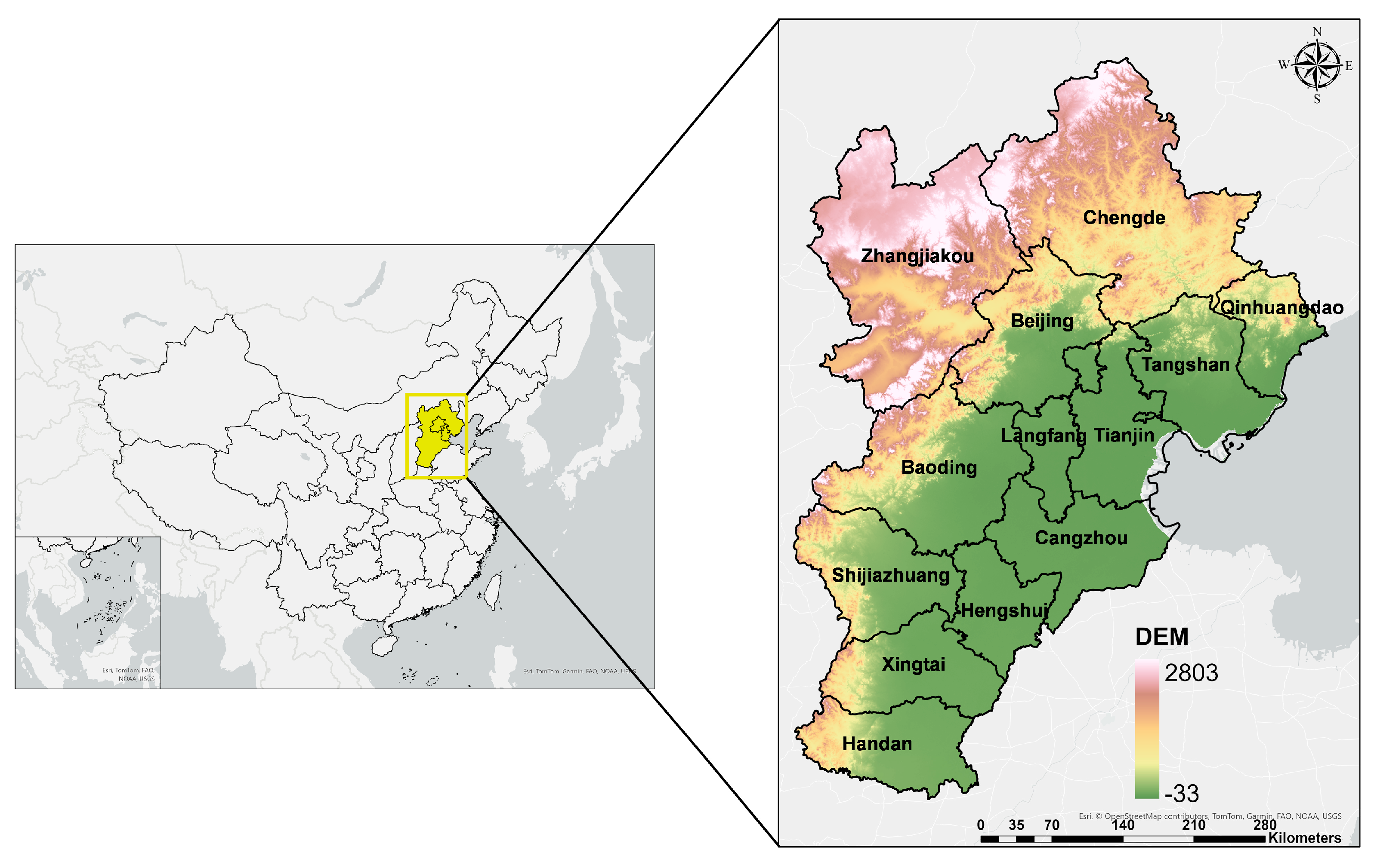
This study was conducted in four parts (Figure 1). The first part mainly included the preprocessing of multiple data records, such as projection adjustment, resampling, and data extraction. Second, we dealt with the nighttime light data (NTL), including dividing NTL into built-up cells (BUCs) to represent the different building centers and their hinterlands in space. Then, the BUCs were divided into USR areas based on annual NTL values using K-means clustering. Third, according to the existing remote sensing data for building volume and built-up land, the horizontal growth and vertical growth of BUCs from 2013 to 2023 were analyzed. The fourth part involved further measuring the comprehensive development intensity (CDI) and the characteristics of horizontal and vertical growth. Finally, we analyzed the factors driving changes in CDI.

2.1. Study Area

For this study, we selected the BTH urban agglomeration as the study area (Figure 2). BTH is one of the major urban agglomerations in China and includes the two municipalities of Beijing and Tianjin and 11 prefecture-level cities in Hebei Province. By the end of 2023, the total population of BTH was about 110 million, accounting for 7.8% of the total population of China. From 2013 to 2023, with the acceleration of urbanization in BTH, the population increased by 1.2 million, the gross domestic product (GDP) increased from CNY 5530 billion to CNY 10,440 billion, and the urbanization rate increased from 72% to 79%, which is higher than the national average urbanization rate of 66%. The overall growth trend of BTH is significant, but there are significant differences within the region. The urbanization rate of Beijing and Tianjin has exceeded 80%, while that of Hebei Province is 63%, indicating that the proportion of rural populations in Hebei Province is still relatively high. At the same time, the urban construction land in Beijing and Tianjin is distributed in a contiguous concentration, while the urban scale and growth rate in Hebei Province are uneven [31]. Therefore, BTH provides rich comparative samples for exploring urban growth patterns in regions at different stages of development.

2.2. Urban Horizontal Growth and Vertical Growth

2.2.1. Division of Built-Up Cells

The density of buildings reflects the intensity of economic activities and population concentration, and it decreases with a decrease in intensity. Previous studies have captured the transitional relationship between the building center and its hinterland using nighttime light data (NTL) to estimate building volume [56,57,58]. The local high and low values of NTL were taken as the “peak” and “valley” of elevation to draw the “watershed” surrounded by local high values, and then the light area was divided into built-up area cells (BUCs) with different shapes. This study referred to methods used in previous studies to estimate the building volume of BUCs in BTH. The above process included the three following steps:

(1)

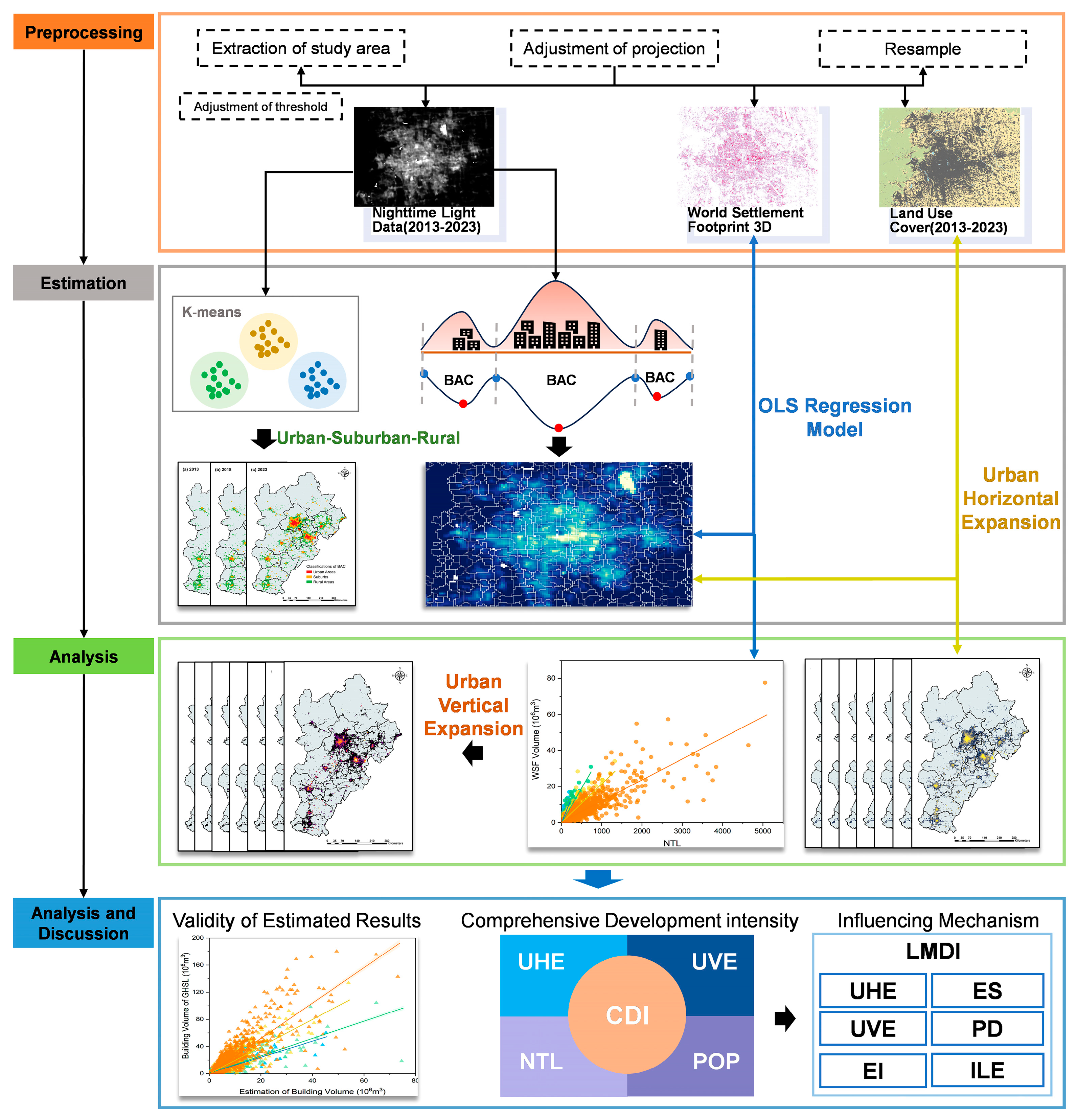
The simulation of valleys and peaks. The pixels with an NTL value of 0 were removed, and the reciprocal of the processed image was used. This means that pixels with low NTL values became larger when processed, while pixels with high NTL values became smaller when processed. They can be regarded as valleys and peaks.

(2)

The confirmation of the flow direction. Flow direction generally goes from peaks to valleys, that is, from high-value areas to low-value areas. By using the flow direction tool of ArcGIS, the direction of each pixel to the steepest descent adjacent point was confirmed according to the D8 flow direction method. The original NTL is the trend of flow from low-value areas to high-value areas, which shows that the low-value areas surround the high-value areas.

(3)

The confirmation of BUCs. The convergence of similar flow directions forms a watershed. Based on the basin analysis tool of ArcGIS, the convergence ranges formed by flow directions with the same convergence points were divided. Regarding the original NTL, the area affected by the same building center was regarded as a convergence range, that is, each convergence range represented the building center and its hinterland. Because the BUCs were used to represent the regional center and hinterland, the BUCs with an area of less than 750,000 square meters were removed from the total sample and finally, 6338 samples were used as research samples.

2.2.2. Estimation of UHE and UVE

Urban horizontal expansion (UHE) refers to the ratio of built-up area to the total area within each cell, as shown in Equation (1).

$${UHE}_i={\displaystyle \frac{{BUA}_i}{{TA}_i}}$$

(1)

where ${BUA}_i$ and ${TA}_i$ refer to the built-up area and total area of BUC $i$, respectively.

Previous studies have used the floor area ratio, calculated using the ratio of floor area to building coverage area and the ratio of horizontal growth to vertical growth, to represent urban vertical growth [30,59]. Therefore, in this study, urban vertical expansion (UVE) was measured using the ratio of floor areas to built-up areas (Equation (2)).

$${UVE}_i={\displaystyle \frac{{FLA}_i}{{BUA}_i}}$$

(2)

where ${UVE}_i$ refers to the vertical growth of BUC $i$ and ${FLA}_i$ refers to the floor area of BUC $i$.

The floor area was calculated by considering the relationship between building volume and height. Previous studies have verified the linear relationship between NTL and the building volume of BUCs [56,57]. In particular, the fitting effect of NTL and building volume was improved after BUCs were grouped according to their luminous efficiency. Therefore, the BUCs in 2013 were grouped according to the luminous efficiency per built-up land area, as shown in Equation (3).

$${\beta }_i={\displaystyle \frac{{NTL}_i}{{BUA}_i}}$$

(3)

where ${\beta }_i$ refers to the luminous efficiency of BUC $i$. The luminous efficiency of buildings varies across different locations. For instance, city centers typically exhibit strong NTL and a large coverage of built-up land, while rural areas display the opposite. The luminous efficiency of all samples was divided into four groups, representing high luminous efficiency, medium–high luminous efficiency, medium–low luminous efficiency, and low luminous efficiency. The sample numbers of each group were kept similar to ensure accurate estimation results. The groups were categorized using the quartile method and divided into four categories in ascending order as follows: 0–25%, 26–50%, 51–75%, and 75–100% (

Table 1. The division of BUCs into groups.

Group	Division Value of β	Average	Median	Number of BUCs
Group 1	17.54	12.50	12.82	1585
Group 2	28.73	22.72	22.54	1584
Group 3	54.08	39.36	37.99	1584
Group 4	11,818	194.70	87.05	1585

). The median luminous efficiency for each group was 12.82, 22.54, 37.99, and 87.05, respectively. The average luminous efficiency for each group was 12.50, 22.72, 39.36, and 194.70. There were significant differences in luminous efficiency across the groups. Moreover, the spatial pattern of groups showed that the closer the area was to the city center, the higher the luminosity (Figure S1). Groups 1, 2, 3, and 4 essentially represent a transition from rural to urban areas, indicating that different luminosity efficiency groups correspond to buildings located in differentiated positions within BTH.

NTL has been proven to have a strong correlation with human socioeconomic activities [60] and is widely used for estimating regional gross domestic product (GDP), population, energy consumption, and other related factors [61,62,63]. Buildings are a key representation of urban development, and previous studies have verified the linear correlation between nighttime light and building systems [57,64]. Therefore, this study determined the linear fitting relationship between NTL and building volume for different groups. Based on the proven linear relationship between NTL and building volume, an OLS regression model was adopted to construct the fitting relation between the observed building volume provided by the World Settlement Footprint 3D (WSF 3D) [54] and NTL among different types of BUCs in 2013 (Equation (4)). The time series for building volume was estimated based on the fitting relation. All the groups showed high fitting results between NTL and building volume, with an R² above 0.7. The groups with samples that had a luminous efficiency of 25–50% and 50–75% showed a better fitting relationship. The estimation models by group are presented in Table S1 and Figure S2. We assumed that the building volume of a BUC has overall positive growth because of the rapid development of the study area from 2013 to 2023, and that the building volume would continue to increase compared to the previous year (Equation (5)). The FLA of each BUC was estimated according to the relationship between building volume and floor height (Equation (6)). Referencing existing studies, a floor height of 3 m was adopted [56].

$${Volume}_i={\alpha }_g\times {NTL}_i+{\theta }_g$$

(4)

$$\left\{\begin{array}{c}{{Volume}_{i,t}=Volume}_{i,t}{ ,Volume}_{i,t}>{Volume}_{i,t-1}\\ {Volume}_{i,t}{=Volume}_{i,t-1} { ,Volume}_{i,t}<{Volume}_{i,t-1}\end{array}\right.$$

(5)

$${FLA}_i={\displaystyle \frac{{Volume}_i}{3}}$$

(6)

where ${Volume}_i$ is the estimated building volume in BUC $i$, ${\alpha }_g$ is the fitting coefficient of group $g$, and ${Volume}_{i,t}$ and ${Volume}_{i,t-1}$ refer to the estimated building volume in $t$ year and $t-1$ year.

2.2.3. Comprehensive Development Intensity

The UHE and UVE represent the physical characteristics of urban growth, while NTL and population serve as indicators of socio-economic intensity. These four variables are integrated to measure the comprehensive development intensity (CDI). The measurement method employed is principal component analysis (PCA). PCA is a widely used statistical technique that condenses a set of variable information into its fundamental features, simplifying it into a few principal components. The principal components are linear combinations of the original variables and are designed to explain the maximum variance across all variables [65]. Two principal components were extracted from the four variables, explaining more than 80% of the variance (Equation (8)). The percentage of variance explained by each principal component was considered as its contribution rate (Equation (9)). Further details can be found in the Supplementary Materials, Table S2.

$${PC}_i=\sum _{j=1}{\gamma }_j{X}_j$$

(7)

$${CDI}_i=\sum _{i=1}{w}_i{PC}_i$$

(8)

where ${PC}_i$ is the $i$-th principal component, ${\gamma }_j$ is the coefficient of factor $X_j$, and $w_i$ is the variance contribution rate of the $i$-th principal component.

2.2.4. Coupling Coordination Analysis

We evaluated the degree of coordination between CDI, population, and economic activities to analyze the rationality of urban growth. The coupling coordination model (CCD) was used to evaluate the coupling coordination between CDI and population and CDI and economic activities, respectively. NTL was used as an indicator of economic activity. The CCD for the CDI and population (POP) was calculated as shown in Equation (9). The classifications of CCD are presented in Table S3.

$$\left\{\begin{array}{c}{C}_i=\sqrt[2]{{\displaystyle \frac{{CDI}_i{POP}_i}{{\left({CDI}_i+{POP}_i\right)}^2}}}\\ T_i={pCDI}_i+{qPOP}_i\\ {CCD}_i=\sqrt{C_i\times T_i}\end{array}\right.$$

(9)

where $C_i$ refers to the coupling degree of BUC $i$ and $T_i$ refers to the coordination degree. $p$ and $q$ are contributions of two systems, which are regarded as weights. According to existing studies, $p=q=0.5$ was adopted [66]. In addition, p = 1/3 and q = 2/3, as well as p = 2/3 and q = 1/3, were adopted to calculate CDI in supplementary situations, which are shown in the Supplementary Materials.

2.2.5. Decomposition of Influencing Factors of Change in CDI

To further analyze the influencing factors of CDI, in this study, we adopted the logarithmic mean Divisa index (LMDI) method to decompose the influencing mechanism of CDI changes in terms of the urban growth pattern and other socioeconomic factors (Equation (10)).

$$CDI={\displaystyle \frac{CDI}{NTL}}\times {\displaystyle \frac{BUA}{TA}}\times {\displaystyle \frac{FLA}{BUA}}\times {\displaystyle \frac{TA}{POP}}\times {\displaystyle \frac{POP}{FLA}}\times NTL=EI\times UHE\times UVE\times PD\times ILE\times ES$$

(10)

${\displaystyle \frac{BUA}{TA}}$ and ${\displaystyle \frac{FLA}{BUA}}$ refer to UHE and UVE, respectively, while ${\displaystyle \frac{CDI}{NTL}}$, ${\displaystyle \frac{TA}{POP}}$, ${\displaystyle \frac{POP}{FLA}}$, and $NTL$ refer to economic intensity, population density, improvement in the living environment, and economic scale, respectively. These were abbreviated as $EI$, $PD$, $ILE$, and $ES$.

2.2.6. Identification of USR Areas

NTL is an effective basis for identifying urban, suburban, and rural areas [67,68]. The similarity of socioeconomic attributes represented by NTL can be used as the basis for the division of different areas. K-means clustering is a widely used classification method. It is based on the input of attribute values of samples and the specified number of categories. In this method, clustering centers are constantly iteratively generated, with samples classified according to the distance between the samples and the center until the average distance within each category reaches a minimum so as to achieve the best classification effect. In this study, the sum of the NTL of each BUC was taken as the attribute value of the input sample, and BUCs were assigned to one of 3 categories, namely urban areas, suburbs, and rural areas. Based on the general transformation of rural areas to suburbs and suburbs to urban areas, the classification results from 2013 to 2023 were further revised. If the classification result was reversed compared with the general transformation direction, it was revised to be the same as the previous year. The number of BUCs of urban areas, suburbs, and rural areas is presented in Table S4. The number of BUCs related to urban areas and suburbs has increased since 2013, but that of rural areas is the opposite. The spatiotemporal distribution of USR areas is shown in Figure S3. The extraction and classification results were compared with published land cover datasets and urban extent datasets [69,70]. The average and median NTL for urban areas, suburbs, and rural areas were used to justify the rationality of the classification. The overall areas extracted in this study showed a high degree of overlap with built-up land and urban extent from existing studies (Figure S4). Significant differences in the average and median NTL were observed between urban areas, suburbs, and rural areas, indicating the effectiveness of the division of these three regions (Figure S5).

2.3. Data Sources

The nighttime light data (NTL) from 2013 to 2023 were derived from the NPP-VIIRS dataset, which was downloaded from the Earth Observation Group website with a resolution of 500 m [71]. The annual data were produced from monthly data. The land use data from 2013 to 2023 used in this study were derived from the published data of related studies with a resolution of 30 m [69], and the built-up land data were extracted as the basis of urban expansion. The building volume data used in this study included data from the World Settlement Footprint 3D (WSF 3D) and the Global Human Settlement Layer (GHSL) BULT-V, both with a resolution of 100 m [54,72,73]. WSF 3D data were used as the 2013 building volume observation data to construct the fitting model with the NTL. GHSL BULT-V data from 2020 were used as validation data to evaluate the accuracy of the estimated building volume results. The population data were downloaded from the WorldPop dataset from 2013 to 2020 with a resolution of 100 m, and the data for 2021 to 2023 were derived according to the average growth rate from 2017 to 2020. The preprocessing of the data was primarily carried out using the ArcGIS platform and involves the following steps: masking and extracting the Beijing–Tianjin–Hebei study area, adjusting to a lambert equal-area projection, and resampling the raster resolution to a 500 m resolution. Based on existing studies, the maximum pixel value of nighttime lights in Beijing was selected as the upper threshold. Nighttime light pixels exceeding this threshold in other cities were adjusted using the mean values of surrounding pixels. Additionally, impervious surfaces were extracted from land use data as the basis for analyzing urban growth (

Table 2. The data used in this study.

Data	Resolution	Sources
Nighttime light data	500 m	https://eogdata.mines.edu/products/vnl/, accessed on 10 September 2024.
Land use data	30 m	https://doi.org/10.5281/zenodo.4417810, accessed on 10 September 2024.
World Settlement Footprint 3D data	100 m	https://download.geoservice.dlr.de/WSF3D/files/, accessed on 26 August 2024.
GHSL BULT-V data	100 m	https://human-settlement.emergency.copernicus.eu/index.php, accessed on 26 August 2024.
WorldPop data	100 m	https://www.worldpop.org/, accessed on 10 October 2024.

).

3. Results

3.1. Characteristics of UHE and UVE

3.1.1. Overall Trends of UHE and UVE

The horizontal expansion area of BTH showed a steady growth trend from 2013 to 2023, increasing from 13.9 billion square meters (m²) to 15.8 billion m² (Figure 3a). The suburbs showed the most significant horizontal expansion, increasing by 2 billion m², followed by urban areas, which increased by 1.4 billion m². In contrast, rural areas were the main land type being transformed into suburbs and urban areas. Therefore, the horizontal expansion of rural areas decreased by 1.6 billion m². In general, the horizontal expansion of BTH was mainly concentrated in the suburbs. However, in terms of the rate of expansion, urban areas expanded at a rate of 165%, far outpacing the 61% rate of expansion in the suburbs. The spatial patterns of horizontal expansion were generally consistent with the above results (Figure S6).

In terms of vertical expansion, the vertical expansion area increased from 4.2 billion m² to 8.3 billion m² from 2013 to 2023 (Figure 3b). Compared with horizontal expansion, the growth scale of vertical expansion was significant. Similarly to horizontal expansion, the vertical expansion of suburbs increased by about 2 billion m², showing the largest growth scale. The vertical expansion area of urban areas increased by 1.3 billion m² but showed the highest growth rate at 226%. The growth scale and growth rate of the vertical expansion area in rural areas were relatively lower. The spatial patterns of vertical expansion are presented in Figure S7. When comparing the growth rate of horizontal expansion and vertical expansion, it can be seen that the vertical growth rate of urban areas and suburbs was higher than the horizontal growth rate in these areas, indicating that the overall density of urban areas and suburbs in BTH has significantly increased.

Figure 3c shows the trend of the ratio of vertical expansion to horizontal expansion (UVE). UVE represents the floor area of built-up areas. A high UVE means that the overall height and density of the region is higher and the intensive development mode is significant. Overall, the UVE values in urban, suburban, and rural areas continued to increase, indicating that density is increasing in all regions. The intensive degree was the highest in urban areas, and the UVE in urban areas increased from 0.59 in 2015 to 0.78 in 2023. The UVE in suburbs increased from 0.35 to 0.6 and showed a gradual upward trend during the study period. The UVE in rural areas increased from 0.26 to 0.40. The comparative results show that the intensive degree of urban areas was further increased due to these areas’ high-density characteristics. Due to the scarcity of central land resources and increased mobility of economic factors and the population, the suburbs had faster horizontal and vertical expansion, and the density of newly developed spaces was significant. Because the rural areas had been transformed into suburbs and even urban areas, the horizontal expansion area of rural areas was relatively smaller, but the floor area increased, which also indicates a vertical growth trend in rural areas.

3.1.2. Spatiotemporal Characteristics of UHE and UVE

The UHE showed a decreasing trend from the city center to outside the city (Figure 4a,b) and the major characteristics of UHE are summarized in Table S5. The land expansion of urban areas reached more than 0.9, indicating a high degree of horizontal development. With the acceleration of urbanization, the areas with UHE values above 0.7 have increased significantly from 2013 to 2023, especially in core areas and the surrounding areas. The UHE surrounding core areas increased at different degrees in each city. Beijing and Tianjin formed a continuous large area of high UHE, and the high-UHE-value area in Shijiazhuang also increased significantly, indicating different degrees of horizontal expansion in each city.

In 2013, the high UVE values were mainly distributed in urban core areas because of the high building density and height (Figure 4c). The UVE value in urban areas was above 0.7, and the UVE values in most peripheral areas were above 0.5 in 2023 (Figure 4d). The major characteristics of UHE are summarized in Table S6. The areas with UVE values above one in Tianjin were still concentrated in the urban areas, but the high-UVE areas in Beijing, Shijiazhuang, Tangshan, and Baoding were scattered in the outer suburbs, being mainly affected by the airport, related infrastructure, and other planning. The overall vertical development further increased, and the trend of outward spread was significant, indicating that with the increase in population and shortage of land resources, the buildings have gradually tended to the attributes of high rise and high density, which improves spatial efficiency.

A comprehensive comparison of the changes in UHE and UVE in urban areas showed that there was less change in the UHE due to the early development of the urban areas. In contrast, the UVE showed significant change, indicating that the urban areas met the urban functional requirements mainly based on vertical growth (Figure 4e). The areas where both UHE and UVE showed significant growth were mainly concentrated in the areas that were further out from the core areas of each city. For example, the urban peripheries of Beijing, Shijiazhuang, and Baoding showed significant changes in UHE and UVE. In contrast, the growth of UHE in the urban peripheries of Tianjin, Tangshan, Cangzhou, Zhangjiakou, Chengde, and Handan was more significant, indicating that the growth of the above areas mainly depended on horizontal expansion and most may be newly developed areas with low density. The field comparison using remote sensing satellite images from Google Earth and the overlapping of UHE and UVE can be referred to in Figures S8 and S9, respectively.

3.2. Analysis of Comprehensive Development Intensity

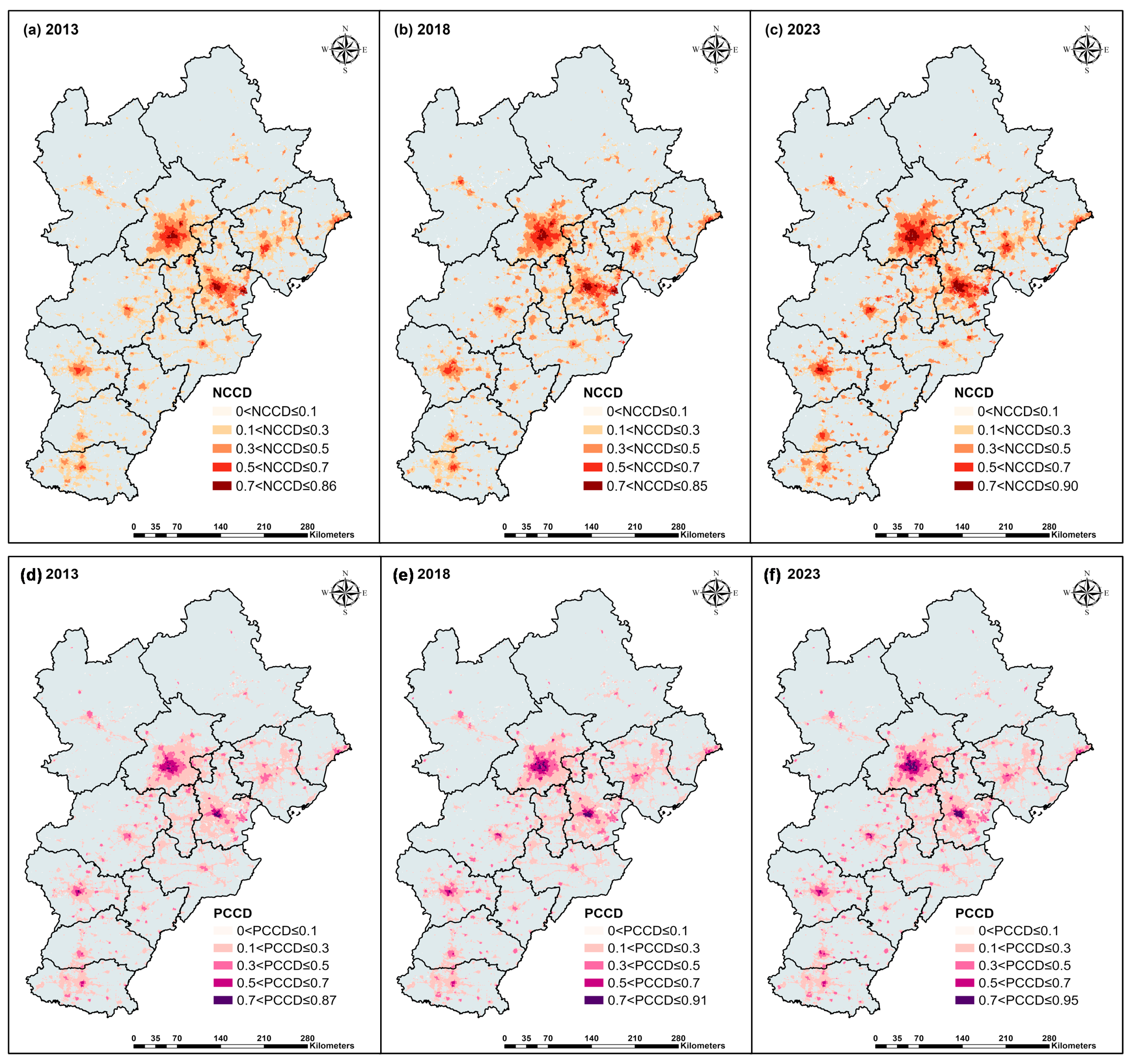
3.2.1. Spatial Characteristics and Changes in CDI

The CDI represents the degree of comprehensive development combined with UHE, UVE, population, and economic activities. The average CDI of BTH increased from 0.12 to 0.15 from 2013 to 2023. The average CDI in urban areas was above 0.4, which is higher than the average CDI in suburbs and rural areas (Figure S10). The CDI in urban areas showed an increasing trend before 2017 and reached a peak of 0.52 in 2016 before decreasing to 0.44 in 2023. The CDI in suburban areas showed a slow downward trend, while the CDI in rural areas showed a trend of fluctuating increase compared with 2013, although the total change was relatively small. The CDI in urban areas and suburbs showed a fluctuating and declining trend, which can be attributed to the effect of the relocation of some industries from urban areas and suburbs and a certain number of low-intensity-development areas. The major characteristics of CDI in urban areas, suburbs, and rural areas are summarized in Table S7.

Regarding spatial features, the CDI patterns from 2013 to 2023 were similar (Figure 5a–c). Areas with high CDI were mainly found in urban areas, and the CDI decreased with increasing distance from urban areas to the suburbs. Beijing, Tianjin, and Shijiazhuang demonstrated relatively high CDIs. Compared with urban areas and suburbs, the CDI increased significantly in rural areas, ranging from below 0.1 to 0.1–0.2 in most areas. From 2013 to 2023, the CDI in most regions showed an increasing trend (Figure 5d). The CDI in suburbs outside the core urban areas of Beijing showed significant growth, while the high-growth areas in other cities were mainly found in the urban areas and surrounding areas. Considering the changes at different time periods, a decline in CDI occurred between 2018 and 2023, with the areas of decline primarily concentrated in suburban and rural regions, as well as some urban areas in Beijing (Figure S11). First, considering the factors used in the calculations, the average population in urban and suburban BUCs significantly decreased after 2018, while the average population in rural areas remained largely unchanged. However, by 2023, there was a noticeable decline in UVE compared to 2018. On one hand, the population in urban and suburban areas continued to disperse, especially after Beijing implemented policies to alleviate non-capital functions, resulting in the relocation of some industries and population. On the other hand, rural areas expanded laterally at a relatively faster pace, leading to a less noticeable increase in UVE.

3.2.2. CCD Between CDI and Economic Activities and Population

The coupling coordination degree of CDI and economic activities (NCCD) in BTH showed an increasing trend from 2013 to 2023 (Figure 6a–c). The NCCD gradually declined with increasing distance from the urban core areas, indicating that the coupling degree of CDI and economic activity intensity of these areas was higher than that of the suburbs. Although the overall NCCD showed an increasing trend, there was still a mismatch between the CDI and economic activity intensity in the suburbs. The high-NCCD area (NCCD > 0.7) and moderate-NCCD area (0.5 < NCCD < 0.7) in Beijing and Tianjin expanded during the research period, indicating that the consistency between the CDI and economic activity intensity in core urban areas and surrounding areas has gradually increased. With an increase in distance from the core areas, the NCCD transitioned from slight disorder to moderate disorder. Similarly, with increasing distance from the core areas, the NCCD of cities in Hebei Province transformed from slight disorder to moderate disorder. Compared with Beijing and Tianjin, the overall NCCD of the cities in Hebei Province was relatively low, and the NCCD of the core area was mainly at a moderate coordination level (0.5 < NCCD < 0.7). In addition, the NCCD with p = 1/3 and q = 2/3 is referred to in Figure S12 and the NCCD with p = 2/3 and q = 1/3 is referred to in Figure S13.

The coupling coordination degree of CDI and population (PCCD) showed a significant growth trend during the research period, with the coordination level of core urban areas and surrounding areas showing the most significant improvement (Figure 6d–f). The high-coordination areas (PCCD > 0.7) were mainly concentrated in the urban areas of Beijing and Tianjin and increased continuously. Meanwhile, there was a trend of moderate disorder to slight disorder and slight disorder to moderate coordination in Beijing and Tianjin. The PCCD in the urban core areas of Hebei Province mainly showed moderate coordination, and the suburbs and rural areas were dominated by slight and moderate disorder. In addition, the PCCD with p = 1/3 and q = 2/3 is referred to in Figure S12 and the PCCD with p = 2/3 and q = 1/3 is referred to in Figure S13.

3.3. Influencing Mechanism of Change in CDI

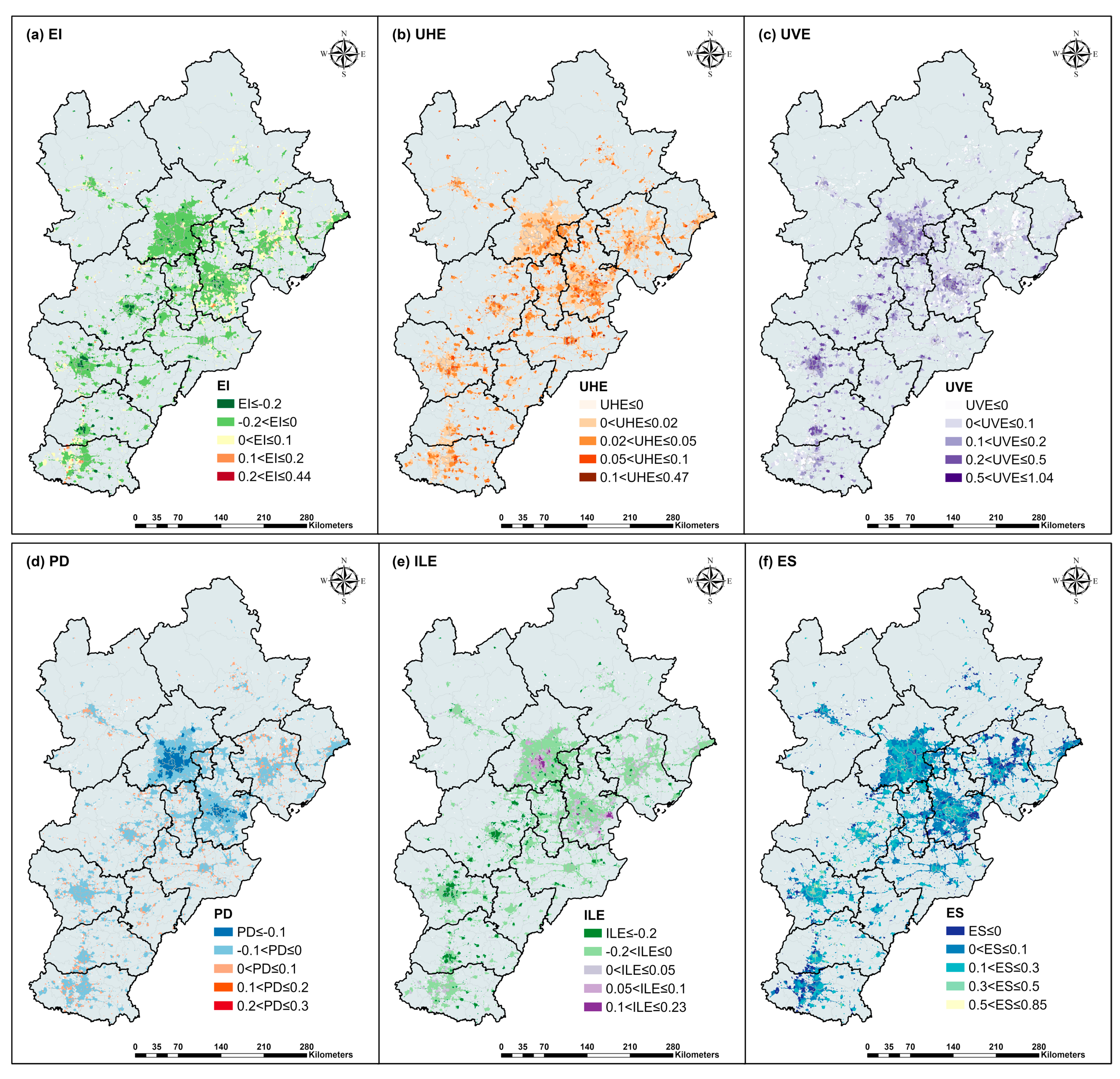
3.3.1. Decomposition of Influencing Factors for Changes in the CDI of BUCs

With the uneven development of urbanization, the change in CDI varied in different regions from 2013 to 2023. Being influenced by the protection of traditional buildings in urban areas, the areas with significant CDI growth in Beijing were mainly concentrated in the periphery of Dongcheng District and Xicheng District. The growth of CDI in Tianjin and Hebei Province, especially in high-growth areas, was mostly centered in urban areas and expanded outward. The changes in these factors are shown in Figure S14. UHE, UVE, and ES were the main positive driving factors (Figure 7b,c,f), and the highly positive effect of UHE was mainly observed in the suburbs, indicating that the suburbs had faster horizontal expansion than the urban areas. The positive impact of UVE was mainly observed in urban areas, which was related to the limited horizontal expansion space and the trend of urban vertical growth of urban areas. The positive effect of ES was also concentrated in urban areas because of the distribution of more commercial and service facilities in these areas.

Economic intensity (EI), population density (PD), and improvement in the living environment (ILE) showed negative effects on CDI changes in most regions (Figure 7a,d,e). EI had a largely negative effect on CDI in most areas, especially urban areas, which indicates that the CDI of NTL decreased in urban areas. On the one hand, the development of urban areas slowed down after 2013. On the other hand, compared with the suburbs, the commercial and service industries were more concentrated in the urban area, and the NTL was more significant. The influencing pattern of PD was similar to that of EI, demonstrating a negative effect in urban areas and a positive effect in a part of the peripheral suburbs, due to the relatively high density, faster growth, and migration of the population in urban areas. ILE showed a positive effect on CDI change in the core urban areas of Beijing and suburbs of other cities, indicating that although the development space in the Beijing urban area was limited and the growth of the floor area was slow, the population growth was relatively faster, so the ILE value increased. The positive effect of ILE in the suburbs of other cities could be attributed to the same reasons. The negative effect of ILE on CDI change in most regions was mainly attributed to the fact that the growth rate of the floor area was higher than that of the population. The decrease in the population per floor area means that the improvement in the living environment has reduced the CDI in most areas.

3.3.2. Decomposition of Influencing Factors by Regions

As can be seen from the average decomposition results during different time periods, ES, UVE, and UHE positively contributed to CDI growth during 2013–2023, and ES and UVE were the main driving factors. EI, ILE, and PD negatively contributed to CDI, and the negative effects of EI and ILE were more significant (Figure 8a). According to our analysis, because the growth of CDI during 2013–2018 was significant, the net contribution of all BUCs during 2013–2018 was 0.022, which was higher than the net contribution of 0.007 observed from 2018 to 2023. The positive driving effect of ES and the negative driving effect of EI were more significant during 2018–2023.

The net contributions of the above factors in urban areas, suburbs, and rural areas from 2013 to 2023 were 0.07, 0.05, and 0.02, respectively (Figure 8b–d). Similarly to the overall trend, ES, UVE, and UHE were the main positive contributing factors. The UVE was the most significant positive contributing factor in each region during the research period, indicating that the increase in urban building density has caused the increase in CDI. EI, PD, and ILE were the main negative factors. EI and ILE demonstrated a negative overall effect, while the negative effect of PD was more significant in urban areas. Comparing the influencing mechanism at different stages of development, the average net contribution of samples from urban areas, the suburbs, and rural areas from 2013 to 2018 was 0.044, 0.04, and 0.02, respectively. The average net contribution of urban areas and the suburbs was similar and higher than the overall average net contribution of BTH, indicating that the CDI was more concentrated in urban areas and suburbs. The average net contribution of urban areas, suburbs, and rural areas from 2018 to 2023 was 0.002, 0.01, and 0.006, respectively. The average net contribution of suburbs and rural areas was higher than that of urban areas, indicating the rapid growth trend of suburbs and rural areas after 2018.

Based on the average contributions of various factors in Beijing, Tianjin, and Hebei Province, it was found that UHE, UVE, and ES contribute positively to the changes in CDI, while EI, PD, and ILE were the main negative contributing factors (Figure S15). This was consistent with the overall CDI influencing mechanism in BTH. Among these factors, the positive contributions of UVE and ES were significantly higher than that of UHE. In Beijing and Hebei Province, the average positive contributions of UVE and ES from 2018 to 2023 were higher than those from 2013 to 2018, reflecting the ongoing trend of urban development. However, the contribution of UVE from 2018 to 2023 was lower than that from 2013 to 2018 in Tianjin, which was related to the slowdown in urban construction in Tianjin. From 2013 to 2023, the differences in the contributions of negative factors between Beijing and Tianjin were minimal, but the negative contribution of ILE in Hebei Province was significantly higher than that in Beijing and Tianjin, while the negative contribution of PD in Hebei was notably lower. This suggested that the growth rate of built-up areas in Hebei Province was faster compared with population growth.

4. Discussion

4.1. Validity and Limitations

By comparing the estimated building volumes for each group with the original WSF3d dataset, it was observed that the groups with low luminous efficiency (below 25%) and high luminous efficiency (above 75%) exhibited greater dispersion in their estimates, whereas the groups in the middle range showed stronger consistency between the estimated and original values (Figure 9a–d). The RMSE of the observed building volume from WSF 3D and estimated volume increased with the improvement in luminous efficiency, indicating that there were more mismatches between the building volume and NTL of large-scale buildings. Overall, 75% of the samples had an RMSE below 1.5, confirming the effectiveness of NTL in estimating building volume. Based on a comparison between the estimated building volume in 2020 and the building volume provided by GHSL in 2020, the estimated results in this study were in high agreement with the results of another dataset, with the R² in all groups above 0.65. The RMSE of 75% of samples was below five, and the RMSE of the group with high luminous efficiency was relatively high. The potential causes of the errors may be attributed to the following three factors:

(1)

For the low-luminous-efficiency group, the errors were more pronounced in the case of BUCs with relatively large-scale building volumes, where most estimations underestimated the actual building volume (Figure 9a). The luminous efficiency groups were mainly located in rural areas with small forms and dispersed distributions (Figure S1). Because of the difficulty in accurately capturing socioeconomic activities in remote areas using NTL, there is a potential for the underestimation of related factors [74,75]. For example, factories or agricultural facilities were generally underestimated in terms of their building volumes. The high-luminous-efficiency group showed both an overestimation and underestimation of building volumes (Figure 9d). The underestimated BUCs in this group were mainly concentrated in the core urban areas, while overestimated BUCs in this group were located in the peripheral areas of the core urban areas (Figure S16). In the core urban areas, NTL cannot always accurately reflect the actual building volume because of the saturation effect, leading to an underestimation of building volumes in the core area. Conversely, the peripheral areas of the core urban areas were affected by nighttime light spillover, causing an overestimation of building volumes in these areas.

(2)

The GHSL building volume data in 2020 were used as validation data. The GHSL building volume dataset was generated by the product of the GHSL built-up surface spatial raster dataset and GHSL building height with a resolution of 100 m [76]. The GHSL built-up surface dataset was mainly derived from Sentinel-2 composite and Landsat multitemporal data. The GHSL building height was derived from AW3D30, SRTM30, and Sentinel-2 composite data (2018). However, the WSF3d data were primarily based on the World Settlement Footprint dataset, amplitude images (TDX-AMP) collected between 2011 and 2013, and the TanDEM-X elevation model (TDX-DEM) with a resolution of 90 m [54]. The differences in data sources, collection times, and methodological frameworks between WSF3d and GHSL led to discrepancies, with GHSL showing higher building volumes compared to WSF3d (Figure 9e–h).

(3)

The groups of luminous efficiency showed a spatial trend of transition from rural to urban centers across Groups 1, 2, 3, and 4. Specifically, the high-luminous-efficiency group primarily included buildings in urban areas. Although the sample numbers were consistent across four groups, the spatial pattern reveals that the high-luminous-efficiency group occupied the largest area. This suggested that the samples in this group were generally larger in building volume. In addition to the saturation and spillover effects of NTL, the larger building volume was one of the reasons why the estimated building volumes for the high-luminous-efficiency group differed significantly from the existing dataset.

4.2. Implications for Sustainable Urban Growth and Planning

Urbanization is a global phenomenon. The flow of people into urban areas has led to greater demand for land to live on and increased urban expansion. The reasonable control and planning of urban growth are of great significance to restrain disorderly sprawl, improve efficiency, and solve ecological and environmental problems. In cities like Portland and London, managing urban boundaries and controlling urban green belts have been effective strategies in controlling urban growth [77,78]. China has experienced rapid urbanization since the 1990s, but the development of urbanization is uneven, as evidenced by both overall inter-city differences and intra-city disparities [79]. The results of this study showed that urban areas have primarily experienced vertical growth in recent years. Meanwhile, as populations and industries have migrated from urban areas, suburban regions have simultaneously undergone rapid horizontal and vertical expansion. The spread and improvement in infrastructure have made the horizontal expansion in rural areas even more pronounced. These differentiated growth patterns have led to varied impacts and offer important insights for regional planning.

At present, urban areas face challenges such as traffic congestion, insufficient land resources, and the need to improve living environments [80]. The high-density urban forms exacerbate the urban heat island effect. In recent years, urban renewal projects, focusing on the renovation of outdated urban infrastructure, housing, and green spaces, have been implemented to optimize functional zoning, beautify urban landscapes, and improve the living experience within limited urban space [81]. Additionally, in East Asian mega-cities such as Tokyo and Seoul, urban growth is gradually transitioning towards a more compact and polycentric urban form. In Beijing, for example, Tongzhou has been designated as a sub-center, with some public service facilities and industries relocated there to supplement the functions of the core urban area. Cities like Tianjin and Shijiazhuang are also gradually shifting to a polycentric structure through the development of the Binhai New Area and Zhengding New Area. This shift is one of the reasons behind the significant horizontal and vertical expansion in suburban areas. However, under a polycentric growth structure, whether vertical growth aligns with actual development needs and whether the functional zoning in the city center is rational will significantly affect the scale of suburban sprawl. At the same time, the extension of infrastructure, such as roads, into suburban areas increases the demand for land and space for commercial, residential, and other functions. Particularly in the context of population and industrial migration, low-density expansion will exacerbate energy consumption and greenhouse gas emissions while consuming green spaces. [38,82]. Therefore, policymakers should strictly regulate land use to prevent suburban land fragmentation and a reduction in compactness. Compact development is thus important to effectively restrain disorderly expansion and improve the efficiency of newly developed land [83]. Rural areas are important to promote urban–rural integration. The significant horizontal expansion indicates an increase in built-up land in rural areas. To ensure ecological protection and food security while promoting economic development in rural areas, it is essential to formulate reasonable plans for infrastructure and unique industries based on the needs of development.

5. Conclusions

In view of the still-evolving research on characterizing the three-dimensional growth characteristics of cities using remote sensing data, this study aims to build a long-term series three-dimensional urban growth analysis framework using NTL, land use data, and building volume data. The results of estimated building volume in BTH showed a high consistency with existing datasets, which verified the effectiveness of this method and can provide reference for future related research. Then, most regions in BTH have experienced horizontal growth and vertical growth from 2013 to 2023, and the total scale of vertical growth was higher. However, the estimation errors were larger in both urban and rural areas. The variables used for estimation can be further enriched based on refining grouping results to improve estimation accuracy in future work. In addition, the method can be adapted to a wider area to validate the estimation method. Based on results, the total vertical expansion scale of the BTH exceeded that of horizontal expansion. Urban areas predominantly experienced vertical growth, while suburban areas showed significant horizontal and vertical expansion and rural areas primarily underwent horizontal expansion. The CDI gradually decreased from the core urban areas, and the growth of CDI from 2013 to 2023 was mainly concentrated in the urban areas and its surrounding area. From the perspective of temporal variation, the growth of CDI was significant from 2013 to 2018, and the growth of CDI after 2018 was slow. The coordination between CDI and economic activities and population was similar to the distribution pattern of CDI. The NCCD and PCCD in urban areas showed high coordination and gradually decreased outward. Based on the analysis results of the influencing mechanism of CDI, it can be found that ES, UHE, and UVE were the main positive influencing factors, while EI, PD, and ILE were the main negative influencing factors. From the perspective of urban planning, due to early development and high-density urban forms, urban renewal can effectively improve the urban environment in urban areas. In addition, the trend towards polycentric structures by developing compact sub-centers can alleviate the issues of high density and congestion in urban areas. In suburbs, where development is rapidly progressing, strict land development policies are needed, along with reasonable functional zoning, to increase suburban compactness and avoid mismatches between planning and actual needs, which can result in low spatial utilization. The plans of rural areas should comprehensively consider both ecological functions and economic functions from the perspectives of unique industries and actual development needs while controlling excessive horizontal expansion caused by infrastructure sprawl.

References

1. Department of Economic and Social Affairs, Population Division World Population Prospects 2024; United Nations: New York, NY, USA, 2024.
2. Seto, K.C.; Güneralp, B.; Hutyra, L.R. Global forecasts of urban expansion to 2030 and direct impacts on biodiversity and carbon pools. Proc. Natl. Acad. Sci. USA 2012, 109, 16083–16088. [Google Scholar] [CrossRef] [PubMed]
3. Martellozzo, F.; Amato, F.; Murgante, B.; Clarke, K.C. Modelling the impact of urban growth on agriculture and natural land in Italy to 2030. Appl. Geogr. 2018, 91, 156–167. [Google Scholar] [CrossRef]
4. Chen, G.; Li, X.; Liu, X.; Chen, Y.; Liang, X.; Leng, J.; Xu, X.; Liao, W.; Qiu, Y.A.; Wu, Q.; et al. Global projections of future urban land expansion under shared socioeconomic pathways. Nat. Commun. 2020, 11, 537. [Google Scholar] [CrossRef] [PubMed]
5. Güneralp, B.; Reba, M.; Hales, B.U.; Wentz, E.A.; Seto, K.C. Trends in urban land expansion, density, and land transitions from 1970 to 2010: A global synthesis. Environ. Res. Lett. 2020, 15, 044015. [Google Scholar] [CrossRef]
6. Chakraborty, S.; Maity, I.; Dadashpoor, H.; Novotnẏ, J.; Banerji, S. Building in or out? Examining urban expansion patterns and land use efficiency across the global sample of 466 cities with million+ inhabitants. Habitat Int. 2022, 120, 102503. [Google Scholar] [CrossRef]
7. He, Q.; Zeng, C.; Xie, P.; Tan, S.; Wu, J. Comparison of urban growth patterns and changes between three urban agglomerations in China and three metropolises in the USA from 1995 to 2015. Sustain. Cities Soc. 2019, 50, 101649. [Google Scholar] [CrossRef]
8. Wu, R.; Li, Z.; Wang, S. The varying driving forces of urban land expansion in China: Insights from a spatial-temporal analysis. Sci. Total Environ. 2021, 766, 142591. [Google Scholar] [CrossRef]
9. Zhang, Q.; Su, S. Determinants of urban expansion and their relative importance: A comparative analysis of 30 major metropolitans in China. Habitat Int. 2016, 58, 89–107. [Google Scholar] [CrossRef]
10. Liang, X.; Liu, X.; Li, X.; Chen, Y.; Tian, H.; Yao, Y. Delineating multi-scenario urban growth boundaries with a CA-based FLUS model and morphological method. Landsc. Urban Plan. 2018, 177, 47–63. [Google Scholar] [CrossRef]
11. Huang, M.; Wang, Z.; Pan, X.; Gong, B.; Tu, M.; Liu, Z. Delimiting China’s Urban Growth Boundaries Under Localized Shared Socioeconomic Pathways and Various Urban Expansion Modes. Earth’s Future 2022, 10, e2021EF002572. [Google Scholar] [CrossRef]
12. Liu, X.; Wang, M.; Qiang, W.; Wu, K.; Wang, X. Urban form, shrinking cities, and residential carbon emissions: Evidence from Chinese city-regions. Appl. Energy 2020, 261, 114409. [Google Scholar] [CrossRef]
13. Wolff, M.; Wiechmann, T. Urban growth and decline: Europe’s shrinking cities in a comparative perspective 1990–2010. Eur. Urban Reg. Stud. 2017, 25, 122–139. [Google Scholar] [CrossRef]
14. Fu, Y.; Li, J.; Weng, Q.; Zheng, Q.; Li, L.; Dai, S.; Guo, B. Characterizing the spatial pattern of annual urban growth by using time series Landsat imagery. Sci. Total Environ. 2019, 666, 274–284. [Google Scholar] [CrossRef] [PubMed]
15. Huang, H.; Chen, P.; Xu, X.; Liu, C.; Wang, J.; Liu, C.; Clinton, N.; Gong, P. Estimating building height in China from ALOS AW3D30. ISPRS J. Photogramm. Remote Sens. 2022, 185, 146–157. [Google Scholar] [CrossRef]
16. Labetski, A.; Vitalis, S.; Biljecki, F.; Arroyo Ohori, K.; Stoter, J. 3D building metrics for urban morphology. Int. J. Geogr. Inf. Sci. 2022, 37, 36–67. [Google Scholar] [CrossRef]
17. Li, X.; Zhou, Y.; Gong, P.; Seto, K.C.; Clinton, N. Developing a method to estimate building height from Sentinel-1 data. Remote Sens. Environ. 2020, 240, 111705. [Google Scholar] [CrossRef]
18. Ren, C.; Cai, M.; Li, X.; Shi, Y.; See, L. Developing a rapid method for 3-dimensional urban morphology extraction using open-source data. Sustain. Cities Soc. 2020, 53, 101962. [Google Scholar] [CrossRef]
19. Frolking, S.; Mahtta, R.; Milliman, T.; Esch, T.; Seto, K.C. Global urban structural growth shows a profound shift from spreading out to building up. Nat. Cities 2024, 1, 555–566. [Google Scholar] [CrossRef]
20. Lemoine-Rodríguez, R.; Inostroza, L.; Zepp, H. The global homogenization of urban form. An assessment of 194 cities across time. Landsc. Urban Plan. 2020, 204, 103949. [Google Scholar] [CrossRef]
21. He, S.; Yu, S.; Li, G.; Zhang, J. Exploring the influence of urban form on land-use efficiency from a spatiotemporal heterogeneity perspective: Evidence from 336 Chinese cities. Land Use Policy 2020, 95, 104576. [Google Scholar] [CrossRef]
22. Güneralp, B.; Zhou, Y.; Ürge-Vorsatz, D.; Gupta, M.; Yu, S.; Patel, P.L.; Fragkias, M.; Li, X.; Seto, K.C. Global scenarios of urban density and its impacts on building energy use through 2050. Proc. Natl. Acad. Sci. USA 2017, 114, 8945–8950. [Google Scholar] [CrossRef]
23. Chen, Y.; Shu, B.; Zhang, R.; Amani-Beni, M. LST determination of different urban growth patterns: A modeling procedure to identify the dominant spatial metrics. Sustain. Cities Soc. 2023, 92, 104459. [Google Scholar] [CrossRef]
24. He, Q.; He, W.; Song, Y.; Wu, J.; Yin, C.; Mou, Y. The impact of urban growth patterns on urban vitality in newly built-up areas based on an association rules analysis using geographical ‘big data’. Land Use Policy 2018, 78, 726–738. [Google Scholar] [CrossRef]
25. Xian, S.; Li, L.; Qi, Z. Toward a sustainable urban expansion: A case study of Zhuhai, China. J. Clean. Prod. 2019, 230, 276–285. [Google Scholar] [CrossRef]
26. Zhao, S.; Zhou, D.; Zhu, C.; Qu, W.; Zhao, J.; Sun, Y.; Huang, D.; Wu, W.; Liu, S. Rates and patterns of urban expansion in China’s 32 major cities over the past three decades. Landsc. Ecol. 2015, 30, 1541–1559. [Google Scholar] [CrossRef]
27. Wu, W.-B.; Yu, Z.-W.; Ma, J.; Zhao, B. Quantifying the influence of 2D and 3D urban morphology on the thermal environment across climatic zones. Landsc. Urban Plan. 2022, 226, 104499. [Google Scholar] [CrossRef]
28. Berger, C.; Rosentreter, J.; Voltersen, M.; Baumgart, C.; Schmullius, C.; Hese, S. Spatio-temporal analysis of the relationship between 2D/3D urban site characteristics and land surface temperature. Remote Sens. Environ. 2017, 193, 225–243. [Google Scholar] [CrossRef]
29. Domingo, D.; van Vliet, J.; Hersperger, A.M. Long-term changes in 3D urban form in four Spanish cities. Landsc. Urban Plan. 2023, 230, 104624. [Google Scholar] [CrossRef]
30. Zambon, I.; Colantoni, A.; Salvati, L. Horizontal vs vertical growth: Understanding latent patterns of urban expansion in large metropolitan regions. Sci. Total Environ. 2019, 654, 778–785. [Google Scholar] [CrossRef]
31. Li, X.; Gong, P.; Zhou, Y.; Wang, J.; Bai, Y.; Chen, B.; Hu, T.; Xiao, Y.; Xu, B.; Yang, J.; et al. Mapping global urban boundaries from the global artificial impervious area (GAIA) data. Environ. Res. Lett. 2020, 15, 094044. [Google Scholar] [CrossRef]
32. He, T.; Wang, K.; Xiao, W.; Xu, S.; Li, M.; Yang, R.; Yue, W. Global 30 meters spatiotemporal 3D urban expansion dataset from 1990 to 2010. Sci. Data 2023, 10, 321. [Google Scholar] [CrossRef] [PubMed]
33. Li, G.; Fang, C.; Li, Y.; Wang, Z.; Sun, S.; He, S.; Qi, W.; Bao, C.; Ma, H.; Fan, Y.; et al. Global impacts of future urban expansion on terrestrial vertebrate diversity. Nat. Commun. 2022, 13, 1628. [Google Scholar] [CrossRef] [PubMed]
34. McDonald, R.I.; Mansur, A.V.; Ascensão, F.; Colbert, M.l.; Crossman, K.; Elmqvist, T.; Gonzalez, A.; Güneralp, B.; Haase, D.; Hamann, M.; et al. Research gaps in knowledge of the impact of urban growth on biodiversity. Nat. Sustain. 2019, 3, 16–24. [Google Scholar] [CrossRef]
35. Lima, G.N.d.; Magaña Rueda, V.O. The urban growth of the metropolitan area of Sao Paulo and its impact on the climate. Weather. Clim. Extrem. 2018, 21, 17–26. [Google Scholar] [CrossRef]
36. Hemmati, M.; Ellingwood, B.R.; Mahmoud, H.N. The Role of Urban Growth in Resilience of Communities Under Flood Risk. Earth’s Future 2020, 8, e2019EF001382. [Google Scholar] [CrossRef] [PubMed]
37. Chuai, X.; Huang, X.; Lu, Q.; Zhang, M.; Zhao, R.; Lu, J. Spatiotemporal Changes of Built-Up Land Expansion and Carbon Emissions Caused by the Chinese Construction Industry. Environ. Sci. Technol. 2015, 49, 13021–13030. [Google Scholar] [CrossRef] [PubMed]
38. VandeWeghe, J.R.; Kennedy, C. A spatial analysis of residential greenhouse gas emissions in the Toronto census metropolitan area. J. Ind. Ecol. 2007, 11, 133–144. [Google Scholar] [CrossRef]
39. Camagni, R.; Gibelli, M.C.; Rigamonti, P. Urban mobility and urban form: The social and environmental costs of different patterns of urban expansion. Ecol. Econ. 2002, 40, 199–216. [Google Scholar] [CrossRef]
40. Mahtta, R.; Fragkias, M.; Güneralp, B.; Mahendra, A.; Reba, M.; Wentz, E.A.; Seto, K.C. Urban land expansion: The role of population and economic growth for 300+ cities. NPJ Urban Sustain. 2022, 2, 5. [Google Scholar] [CrossRef]
41. Li, C.; Li, J.; Wu, J. What drives urban growth in China? A multi-scale comparative analysis. Appl. Geogr. 2018, 98, 43–51. [Google Scholar] [CrossRef]
42. Jing, S.; Yan, Y.; Niu, F.; Song, W. Urban Expansion in China: Spatiotemporal Dynamics and Determinants. Land 2022, 11, 356. [Google Scholar] [CrossRef]
43. Li, X.; Zhou, W.; Ouyang, Z. Forty years of urban expansion in Beijing: What is the relative importance of physical, socioeconomic, and neighborhood factors? Appl. Geogr. 2013, 38, 1–10. [Google Scholar] [CrossRef]
44. Deng, Y.; Fu, B.; Sun, C. Effects of urban planning in guiding urban growth: Evidence from Shenzhen, China. Cities 2018, 83, 118–128. [Google Scholar] [CrossRef]
45. Lei, Y.; Flacke, J.; Schwarz, N. Does Urban planning affect urban growth pattern? A case study of Shenzhen, China. Land Use Policy 2021, 101, 105100. [Google Scholar] [CrossRef]
46. Dinda, S.; Das Chatterjee, N.; Ghosh, S. An integrated simulation approach to the assessment of urban growth pattern and loss in urban green space in Kolkata, India: A GIS-based analysis. Ecol. Indic. 2021, 121, 107178. [Google Scholar] [CrossRef]
47. Das, S.; Jain, G.V. Assessment and Prediction of Urban Expansion Using CA-Based SLEUTH Urban Growth Model: A Case Study of Kolkata Metropolitan Area (KMA), West Bengal, India. J. Indian Soc. Remote Sens. 2022, 50, 2277–2302. [Google Scholar] [CrossRef]
48. Shahfahad; Naikoo, M.W.; Towfiqul Islam, A.R.M.; Mallick, J.; Rahman, A. Land use/land cover change and its impact on surface urban heat island and urban thermal comfort in a metropolitan city. Urban Clim. 2022, 41, 101052. [Google Scholar] [CrossRef]
49. Basu, T.; Das, A.; Pereira, P. Exploring the drivers of urban expansion in a medium-class urban agglomeration in India using the remote sensing techniques and geographically weighted models. Geogr. Sustain. 2023, 4, 150–160. [Google Scholar] [CrossRef]
50. Padon, A.; Iamtrakul, P.; Thanapirom, C. The Study of Urbanization Effect on the Land Use Changes and Urban Infrastructures Development in the Metropolitan Areas, Thailand. IOP Conf. Ser. Earth Environ. Sci. 2021, 738, 012077. [Google Scholar] [CrossRef]
51. Nishiura, S.; Leeruttanawisut, K. Evolution of subcenter structure in Bangkok metropolitan development from 1988 to 2018. Appl. Geogr. 2022, 145, 102715. [Google Scholar] [CrossRef]
52. Sono, D.; Wei, Y.; Chen, Z.; Jin, Y. Spatiotemporal Evolution of West Africa’s Urban Landscape Characteristics Applying Harmonized DMSP-OLS and NPP-VIIRS Nighttime Light (NTL) Data. Chin. Geogr. Sci. 2022, 32, 933–945. [Google Scholar] [CrossRef]
53. Shohan, A.A.A.; Bindajam, A.; Al-Shayeb, M.; Thi, H. Assessing urban growth through morphological spatial pattern analysis in cloud computing platform. Front. Eng. Built Environ. 2024, 4, 215–229. [Google Scholar] [CrossRef]
54. Esch, T.; Brzoska, E.; Dech, S.; Leutner, B.; Palacios-Lopez, D.; Metz-Marconcini, A.; Marconcini, M.; Roth, A.; Zeidler, J. World Settlement Footprint 3D—A first three-dimensional survey of the global building stock. Remote Sens. Environ. 2022, 270, 112877. [Google Scholar] [CrossRef]
55. Liu, Z.; Tang, H.; Feng, L.; Lyu, S. China Building Rooftop Area: The first multi-annual (2016–2021) and high-resolution (2.5 m) building rooftop area dataset in China derived with super-resolution segmentation from Sentinel-2 imagery. Earth Syst. Sci. Data 2023, 15, 3547–3572. [Google Scholar] [CrossRef]
56. Liang, H.; Bian, X.; Dong, L.; Shen, W.; Chen, S.S.; Wang, Q. Mapping the evolution of building material stocks in three eastern coastal urban agglomerations of China. Resour. Conserv. Recycl. 2023, 188, 106651. [Google Scholar] [CrossRef]
57. Peled, Y.; Fishman, T. Estimation and mapping of the material stocks of buildings of Europe: A novel nighttime lights-based approach. Resour. Conserv. Recycl. 2021, 169, 105509. [Google Scholar] [CrossRef]
58. Zhao, F.; Wu, H.; Zhu, S.; Zeng, H.; Zhao, Z.; Yang, X.; Zhang, S. Material stock analysis of urban road from nighttime light data based on a bottom-up approach. Environ. Res. 2023, 228, 115902. [Google Scholar] [CrossRef]
59. Wang, N.; Chen, Z.; Li, T.; Zhen, M. Spatiotemporal Pattern Evolution and Influence Mechanism of Urban Vertical Expansion: A Case Study of Jiangsu Province, China. Land 2022, 11, 433. [Google Scholar] [CrossRef]
60. Henderson, J.V.; Storeygard, A.; Weil, D.N. Measuring economic growth from outer space. Am. Econ. Rev. 2012, 102, 994–1028. [Google Scholar] [CrossRef] [PubMed]
61. Li, S.; Cheng, L.; Liu, X.; Mao, J.; Wu, J.; Li, M. City type-oriented modeling electric power consumption in China using NPP-VIIRS nighttime stable light data. Energy 2019, 189, 116040. [Google Scholar] [CrossRef]
62. Stathakis, D.; Baltas, P. Seasonal population estimates based on night-time lights. Comput. Environ. Urban Syst. 2018, 68, 133–141. [Google Scholar] [CrossRef]
63. Zhou, N.; Hubacek, K.; Roberts, M. Analysis of spatial patterns of urban growth across South Asia using DMSP-OLS nighttime lights data. Appl. Geogr. 2015, 63, 292–303. [Google Scholar] [CrossRef]
64. Shi, L.; Foody, G.M.; Boyd, D.S.; Girindran, R.; Wang, L.; Du, Y.; Ling, F. Night-time lights are more strongly related to urban building volume than to urban area. Remote Sens. Lett. 2020, 11, 29–36. [Google Scholar] [CrossRef]
65. Greenacre, M.; Groenen, P.J.F.; Hastie, T.; D’Enza, A.I.; Markos, A.; Tuzhilina, E. Principal component analysis. Nat. Rev. Methods Primers 2022, 2, 100. [Google Scholar] [CrossRef]
66. Chen, J.; Li, Z.; Dong, Y.; Song, M.; Shahbaz, M.; Xie, Q. Coupling coordination between carbon emissions and the eco-environment in China. J. Clean. Prod. 2020, 276, 123848. [Google Scholar] [CrossRef]
67. Huang, Y.; Yang, J.; Chen, M.; Wu, C.; Ren, H.; Liu, Y. An Approach for Retrieving Consistent Time Series “Urban Core–Suburban-Rural” (USR) Structure Using Nighttime Light Data from DMSP/OLS and NPP/VIIRS. Remote Sens. 2022, 14, 3642. [Google Scholar] [CrossRef]
68. Liu, S.; Shi, K.; Wu, Y. Identifying and evaluating suburbs in China from 2012 to 2020 based on SNPP–VIIRS nighttime light remotely sensed data. Int. J. Appl. Earth Obs. Geoinf. 2022, 114, 103041. [Google Scholar] [CrossRef]
69. Yang, J.; Huang, X. The 30 m annual land cover dataset and its dynamics in China from 1990 to 2019. Earth Syst. Sci. Data 2021, 13, 3907–3925. [Google Scholar] [CrossRef]
70. Zhao, M.; Cheng, C.; Zhou, Y.; Li, X.; Shen, S.; Song, C. A global dataset of annual urban extents (1992–2020) from harmonized nighttime lights. Earth Syst. Sci. Data 2022, 14, 517–534. [Google Scholar] [CrossRef]
71. Chen, Z.; Yu, B.; Yang, C.; Zhou, Y.; Yao, S.; Qian, X.; Wang, C.; Wu, B.; Wu, J. An extended time series (2000–2018) of global NPP-VIIRS-like nighttime light data from a cross-sensor calibration. Earth Syst. Sci. Data 2021, 13, 889–906. [Google Scholar] [CrossRef]
72. Wu, B.; Huang, H.; Wang, Y.; Shi, S.; Wu, J.; Yu, B. Global spatial patterns between nighttime light intensity and urban building morphology. Int. J. Appl. Earth Obs. Geoinf. 2023, 124, 103495. [Google Scholar] [CrossRef]
73. Pesaresi, M.; Politis, P. GHS-BUILT-V R2023A-GHS Built-Up Volume Grids Derived from Joint Assessment of Sentinel2, Landsat, and Global DEM Data, Multitemporal (1975–2030). 2023. Available online: https://data.jrc.ec.europa.eu/dataset/ab2f107a-03cd-47a3-85e5-139d8ec63283 (accessed on 2 February 2025).
74. Li, X.; Zhou, W. Dasymetric mapping of urban population in China based on radiance corrected DMSP-OLS nighttime light and land cover data. Sci. Total Environ. 2018, 643, 1248–1256. [Google Scholar] [CrossRef] [PubMed]
75. Mellander, C.; Lobo, J.; Stolarick, K.; Matheson, Z. Night-Time Light Data: A Good Proxy Measure for Economic Activity? PLoS ONE 2015, 10, e0139779. [Google Scholar] [CrossRef] [PubMed]
76. Schiavina, M.; Melchiorri, M.; Pesaresi, M.; Politis, P.; Freire, S.; Maffenini, L.; Florio, P.; Ehrlich, D.; Goch, K.; Tommasi, P. GHSL Data Package 2022; Publications Office of the European Union: Luxembourg, 2022. [Google Scholar]
77. Gillham, O. The Limitless City: A Primer on the Urban Sprawl Debate; Island Press: Washington, DC, USA, 2002. [Google Scholar]
78. Shlomo, A.; Parent, J.; CIVCO, L.; Blei, A. Making Room for a Planet of Cities; The Lincoln Institute of Land Policy: Cambridge, MA, USA, 2011. [Google Scholar]
79. Ye, C.; Chen, M.; Duan, J.; Yang, D. Uneven development, urbanization and production of space in the middle-scale region based on the case of Jiangsu province, China. Habitat Int. 2017, 66, 106–116. [Google Scholar] [CrossRef]
80. Yıldız, S.; Kıvrak, S.; Gültekin, A.B.; Arslan, G. Built environment design-social sustainability relation in urban renewal. Sustain. Cities Soc. 2020, 60, 102173. [Google Scholar] [CrossRef]
81. Wang, Y.; Fan, Y.; Yang, Z. Challenges, Experience, and Prospects of Urban Renewal in High-Density Cities: A Review for Hong Kong. Land 2022, 11, 2248. [Google Scholar] [CrossRef]
82. Xu, C.; Haase, D.; Su, M.; Yang, Z. The impact of urban compactness on energy-related greenhouse gas emissions across EU member states: Population density vs physical compactness. Appl. Energy 2019, 254, 113671. [Google Scholar] [CrossRef]
83. Wu, H.; Fang, S.; Zhang, C.; Hu, S.; Nan, D.; Yang, Y. Exploring the impact of urban form on urban land use efficiency under low-carbon emission constraints: A case study in China’s Yellow River Basin. J. Environ. Manag. 2022, 311, 114866. [Google Scholar] [CrossRef]
Figure 1. Research flow of this study.
Remotesensing 17 00548 g001
Figure 2. The location and DEM of the Beijing–Tianjin–Hebei urban agglomeration. BTH contains 13 cities.
Remotesensing 17 00548 g002
Figure 3. Trend of horizontal expansion and vertical expansion. (ac) Horizontal expansion, vertical expansion, and UVE in urban areas, suburbs, and rural areas.
Remotesensing 17 00548 g003
Figure 4. Spatial characteristics and changes in UHE and UVE. (a,b) UHE, (c,d) UVE, (e) overlapping of change in UHE and UVE.
Remotesensing 17 00548 g004
Figure 5. Spatial characteristics and changes in CDI. (ac) CDI in 2013, 2018, and 2023. (d) Change of CDI between 2013 and 2023.
Remotesensing 17 00548 g005
Figure 6. Spatial characteristics of NCCD and PCCD. (ac) NCCD in 2013, 2018, and 2023. (df) PCCD in 2013, 2018, and 2023.
Remotesensing 17 00548 g006
Figure 7. Decomposition of influencing factors of changes in CDI from 2013 to 2023. (af) EI, UHE, UVE, PD, ILE, and ES, which represent economic intensity, horizontal expansion, vertical expansion, population density, improvement in the living environment, and economic scale, respectively.
Remotesensing 17 00548 g007
Figure 8. Average contribution of factors by region and research period. (a) The decomposition of influencing factors of BTH. (bd) The decomposition of influencing factors in urban areas, suburbs, and rural areas.
Remotesensing 17 00548 g008
Figure 9. The validity of estimation building volume in this study. (ad) A comparison between estimated results with WSF3d in 2013. (eh) A comparison between estimated results with GHSL in 2020.
Remotesensing 17 00548 g009