A Comparative Study of Downscaling Methods for Groundwater Based on GRACE Data Using RFR and GWR Models in Jiangsu Province, China

Abstract

The Gravity Recovery and Climate Experiment (GRACE) introduces a new approach to accurately monitor, in real time, regional groundwater resources, which compensates for the limitations of traditional hydrological observations in terms of spatiotemporal resolution. Currently, observations of groundwater storage changes in Jiangsu Province face issues such as low spatial resolution, limited applicability of the downscaling models, and insufficient water resource observation data. This study based on GRACE employs Random Forest Regression (RFR) and Geographically Weighted Regression (GWR) methods in order to obtain high-resolution information on groundwater storage change. The results indicate that among the established 66 × 158 local GWR models, the coefficient of determination (R²) ranges from 0.39 to 0.88, with a root mean squared error (RMSE) of approximately 2.60 cm. The proportion of downscaling models with an R² below 0.5 was 18.52%. Similarly, the RFR models trained on the above time series grid data achieved an R² of 0.50, with the RMSE fluctuating around 1.59 cm. In the results validation, the monthly correlation coefficients between the GWR downscaling results and the data of measured stations ranged from 0.37 to 0.66, with 53.33% of the stations having a coefficient greater than 0.5. The seasonal correlation coefficients ranged from 0.41 to 0.62, with 60% of the stations exceeding 0.5. The correlation coefficients for the RFR downscaling results ranged from 0.44 to 0.88, with seasonal correlation coefficients ranging from 0.49 to 0.84. Only one station had a correlation coefficient below 0.5 for both monthly and seasonal results. In the validation of the correlation accuracy between the downscaling results and the measured groundwater levels, the Random Forest model demonstrated better predictive performance, which offers distinct advantages in improving the spatial resolution of groundwater storage changes in Jiangsu Province.

1. Introduction

Water resources, as some of the most dynamic elements of nature, are the basis for human life, economic activity, and the sustainable development of ecosystems [1,2,3]. As an important component of freshwater resources, the distribution and changes in groundwater are intricately linked to human activities. In recent years, against the backdrop of climate change, the increasing frequency of extreme droughts and floods, and the unsustainable use of groundwater resources by human beings [4,5], the changes in groundwater reserves and their monitoring have become increasingly important [6], holding a significant position in the new natural resource survey and monitoring system [3].

With the continuous development of geophysics and the improvement of satellite remote sensing technology and hydrological models, GRACE satellites offer a new approach for monitoring terrestrial water storage [7,8,9] and groundwater storage changes [10,11,12] by capturing subtle variations in the Earth’s gravity field on a global scale. This enables the dynamic monitoring of groundwater storage from global to regional and watershed scales, providing valuable groundwater data [13]. Rana et al. used GRACE data in conjunction with climate and socio-economic datasets to analyze the spatiotemporal characteristics of groundwater changes in northern India over the past two decades, as well as the interactions between climate, socio-economic factors, and groundwater [14]. Yoshe et al. investigated the spatiotemporal variation of water storage in Ethiopia using GRACE data combined with the Global Land Data Assimilation System (GLDAS), with a focus on the seasonal variations in the time series of surface water [15]. Cho et al. utilized Google Earth Engine (GEE) to analyze variations in terrestrial water storage in South Korea [16]. Although GRACE has demonstrated irreplaceable advantages in analyzing and calculating water storage changes in large-scale areas (ranging from approximately 45,000 km² to 600,000 km²), its low spatial resolution (0.25 × 0.25° to 1 × 1°) and the need for monitoring small-scale terrestrial water storage highlight the necessity of employing effective methods to enhance the spatial resolution of GRACE products.

At present, downscaling GRACE satellite data with coarse-resolution by integrating hydrological and meteorological data is an effective approach to obtaining high-resolution groundwater data over large areas [17]. Therefore, previous studies have conducted extensive works to improve the spatial resolution of GRACE satellite data through downscaling methods, which can be broadly classified into two categories: (1) dynamic downscaling based on physical models [18] and (2) statistical downscaling based on feature data. The research utilizing dynamic downscaling methods to simulate terrestrial water storage change is highly dependent on hydrological models [19], typically employing techniques such as ensemble Kalman filtering and smoothing [20] to assimilate GRACE data into hydrological models [21]. Due to the unavailability of some model data and the complexity of downscaling processes in dynamic models, it is challenging for most researchers to access them. Therefore, the promotion and application of dynamic downscaling methods face certain difficulties and limitations. In contrast, statistical downscaling methods are relatively simple, typically establishing linear or nonlinear relationships between input and output variables. These methods typically assume that the statistical relationship between the variables remains unchanged before and after the change in spatial resolution [22]. The process involves first constructing a statistical model and mapping the relationship between groundwater storage and certain explanatory variables at a coarser spatial resolution. Subsequently, downscaling is performed by applying the mapping relationship to a high-resolution feature dataset [23].

It is generally acknowledged that the complex hydrological processes governing the relationship between groundwater storage and various hydro-meteorological factors cannot be effectively captured by simple linear models. Consequently, machine learning methods, renowned for their exceptional performance in addressing nonlinear regression problems, have been widely applied in downscaling efforts. Currently, statistical downscaling methods, especially machine learning models (such as Support Vector Machine (SVM) [24], Extreme Gradient Boosting (XGBoost) [25], Random Forest regression (RFR) [26,27], etc.), are primarily used to derive high-resolution GRACE data. Ali et al. compared the downscaling results of XGBoost and Artificial Neural Network (ANN) and used them for drought severity assessment, with the XGBoost model yielding the most optimal performance [28]. Kalu et al. evaluated the downscaling performance of Partial Least Squares (PLS), Gaussian Process (GP), SVM, and RF in the western region of Australia. Among these, the RF method achieved the best accuracy [29]. Wang et al. used RF to downscale groundwater across vast regions of Sub-Saharan Africa, the Middle East, and South Asia from 3° to 0.25°, and the results demonstrated the strong robustness of the RF model [30]. These studies highlight the outstanding accuracy of ensemble learning models, especially the RF model, in groundwater downscaling tasks. In addition, some studies account for the spatial heterogeneity of groundwater storage and the variability of aquifers, opting to use spatially explicit modeling approaches. Huang et al. used the Geographically Weighted Regression (GWR) model for groundwater storage downscaling, successfully reducing the spatial resolution of groundwater storage changes in the Hai River Basin, China, to 1 km [31]. Similarly, Zhiwei Chen applied GWR to perform spatial downscaling for the Tarim Basin and Qaidam Basin in China [32]. Yazdian et al. proposed a Spatially Enhanced Support Vector Machine (SP-SVM) model that uses the distance between unknown target points and surrounding GRACE data points as inputs, downscaling GRACE data from 0.5° to 0.25° [24].

In recent years, there have been numerous applications and results in estimating regional and even global groundwater storage changes based on GRACE data and various hydrological models such as the GLDAS. However, due to differences in administrative boundaries, many water resource surveys and monitoring activities are conducted based on administrative units rather than geographic units commonly referenced in studies, such as river basins or aquifer regions. Within the same administrative unit, multiple relatively independent geographic units may exist, and the location of aquifers may change with spatial variations [13]. Therefore, conducting model performance comparisons in such complex units can provide a better assessment of the robustness of models like RFR and GWR, offering valuable insights for downscaling groundwater data in regions with non-uniform geographic structures. Meanwhile, this study uses RFR and GWR algorithms as examples to compare spatially explicit models with traditional statistical models [33]. It evaluates model performance at a fine spatial resolution (0.01°), compares the distribution and patterns of model errors across space, and assesses the applicability of the models in different scenarios, providing useful references for future applications.

2. Study Area and Datasets

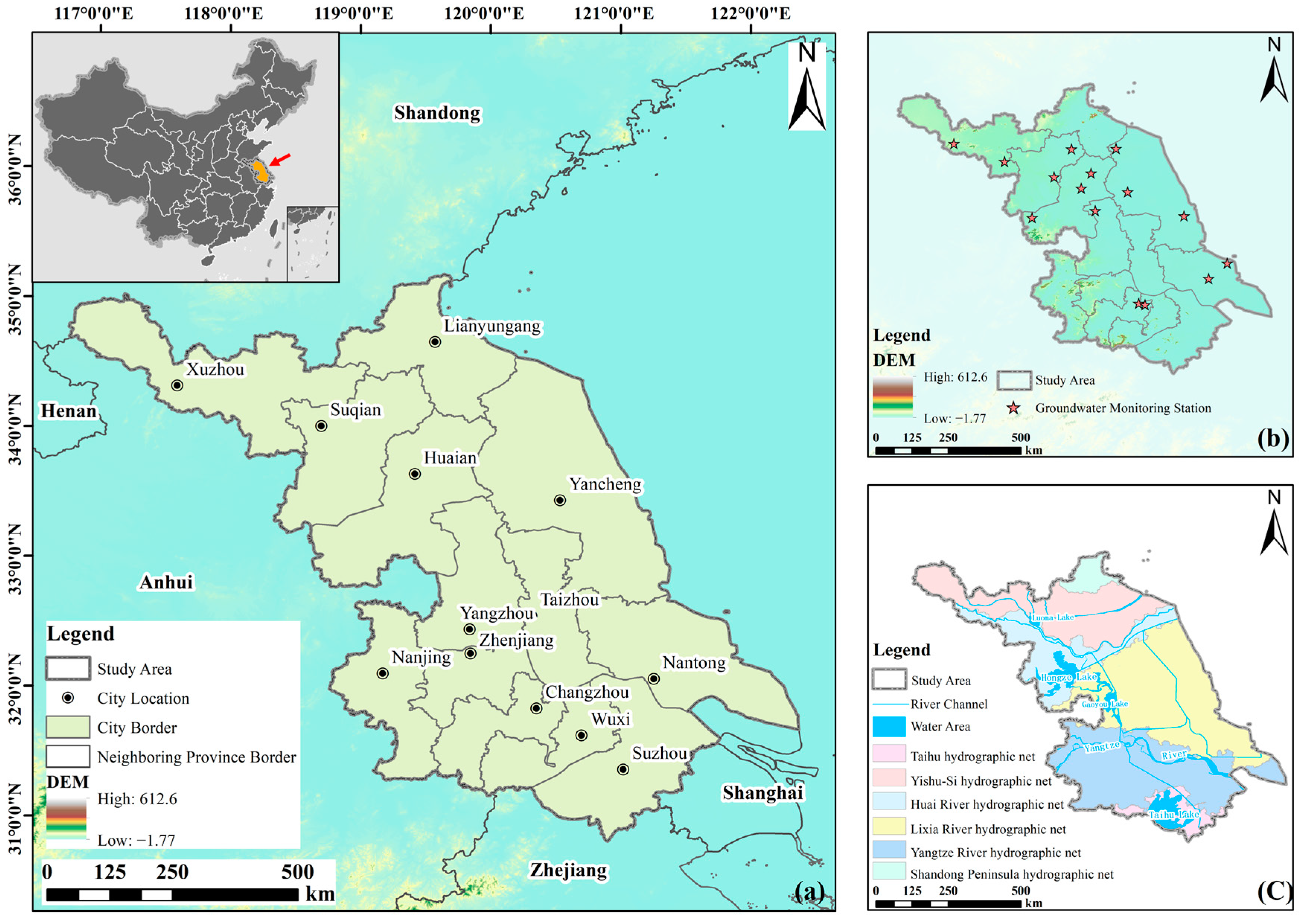
2.1. Study Area

As shown in Figure 1, Jiangsu Province is located in the eastern coastal region of China, situated in the lower reaches of the Yangtze River, with elevations ranging from 0 to 625 m. The terrain within the province primarily consists of plains, low hills, and mountainous areas. Jiangsu Province governs 13 cities. It is characterized by its extensive rivers and lakes, dense water networks, and proximity to both sea and land, with water areas accounting for approximately 16.9% of the province’s total area. According to the 2023 Jiangsu Province Water Resources Bulletin, the annual precipitation in the province is 813.3 mm, with a total water resource volume of 19.28 billion cubic meters, of which groundwater resources amount to 10.27 billion cubic meters [34].

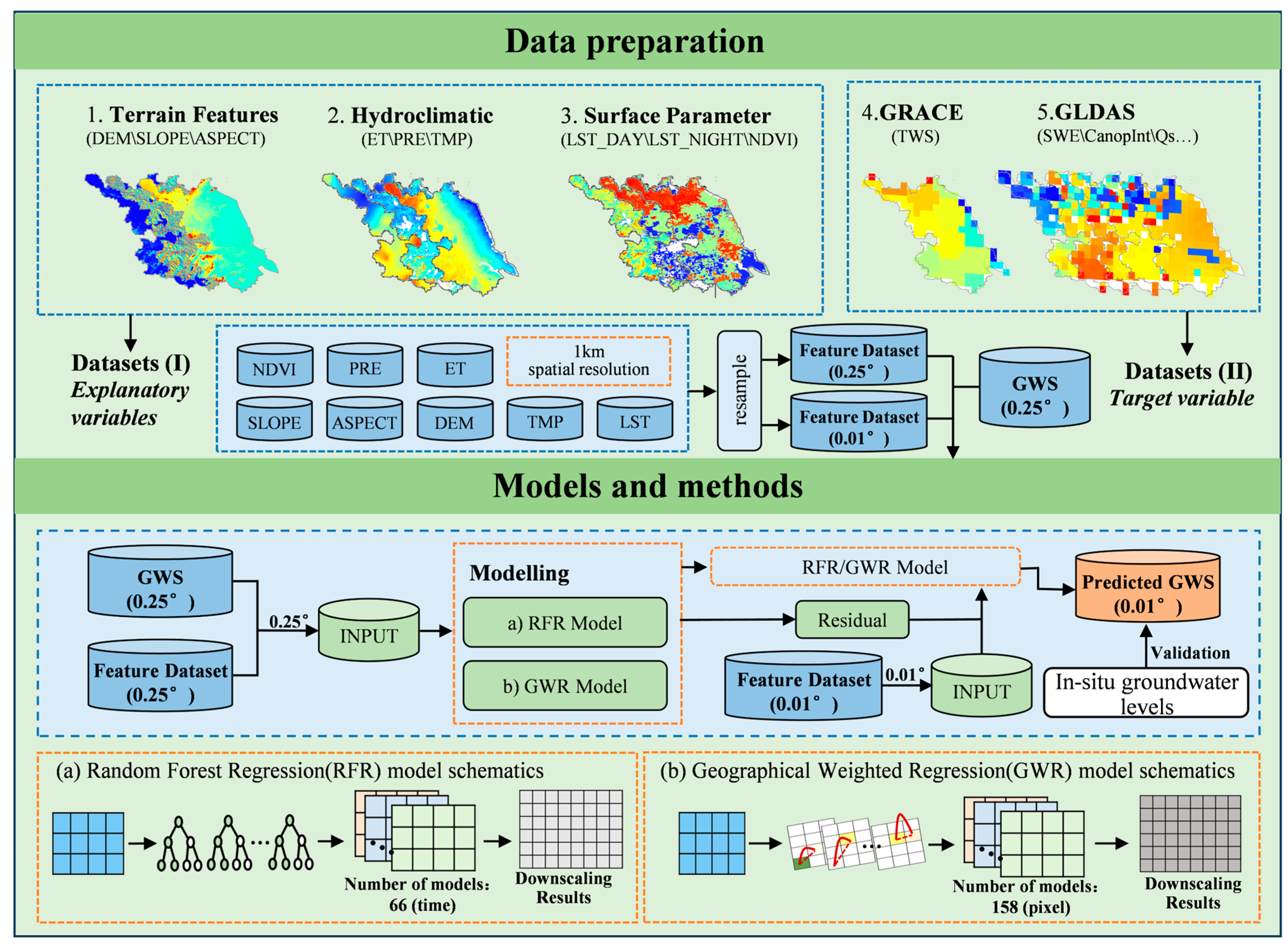
2.2. Research Framework

As shown in the research framework in Figure 2, this study first resampled nine feature variables to a spatial resolution of 0.25° in order to match the resolution of gravity satellite-derived groundwater storage data. Following data preparation, GWR and RFR models were trained using groundwater storage change (expressed as equivalent water height) as the target variable to establish a robust predictive framework. Finally, the high spatial resolution feature variables of 0.01° were used to input the mode, since the statistical relationships established in the lower-resolution models remain applicable at the high-resolution scale and high-resolution predictions of changes in groundwater storage are obtained. Additionally, since the regression models cannot explain all variations in groundwater storage, residuals were added to the high-resolution regression results to obtain the final downscaled groundwater storage results.

2.3. Data Source

This study primarily uses six datasets: (1) GRACE/GRACE-FO dataset product; (2) GLDAS Noah hydrological model dataset product; (3) temperature and precipitation dataset; (4) MODIS dataset; (5) observational data from groundwater monitoring stations [35,36,37,38]; and (6) basic geographic information data. For a comprehensive understanding of the data utilized in our study, please refer to

Table 1. Multi-source datasets and related information statistics.

Dataset	Variable Name	Spatial (Temporal) Resolution	Source
GRACE Mascon (CSR RL06M)	Terrestrial Water Storage (TWS)	0.25° (monthly)	https://www2.csr.utexas.edu/grace (accessed on 16 September 2023)
GLDAS Noah v2.1	Soil moisture (SM)	0.25° (monthly)	https://disc.gsfc.nasa.gov/datasets/ (accessed on 28 August 2023)
	Snow depth water equivalent (SWE_inst)	0.25° (monthly)
	Plant canopy surface water (CanopInt_inst)	0.25° (monthly)
	Storm surface runoff (QS_acc)	0.25° (monthly)
TPDC Temperature and precipitation dataset	Precipitation (Pre)	1 km (monthly)	https://data.tpdc.ac.cn/ (accessed on 19 December 2023)
	Temperature (Tmp)	1 km (monthly)
MODIS 13A3	Normalized Difference Vegetation Index (NDVI)	1 km (8 days)	https://search.earthdata.nasa.gov (accessed on 20 August 2023)
MODIS 16A2	Evapotranspiration (ET)	1 km (8 days)
MODIS 11A2	Land Surface Temperature (LST)	1 km (8 days)
Groundwater level dataset	Ground observations	Stations (monthly)	Annual Report on Groundwater Levels Monitoring of Geological Environment in China

, which provides detailed information on the various datasets employed.

2.3.1. GRACE Mascon Products

GRACE is a satellite project developed with collaboration between the National Aeronautics and Space Administration (NASA) of the United States and the German Aerospace Center (Deutsches Zentrum für Luft- und Raumfahrt, DLR). GRACE aims to provide a new method for monitoring and estimating global water resource changes. Currently, the GRACE satellite data products used for studying changes in the Earth’s water storage mainly include spherical harmonic coefficient data and GRACE Mascon data. In this study, we utilize the GRACE/GRACE-FO Mascon data provided by CSR to estimate changes in terrestrial water storage in Jiangsu Province, covering the time span from April 2002 to April 2023, with a total of 218 months after excluding the months with missing data.

2.3.2. GLDAS Model Products

The Global Land Data Assimilation System (GLDAS), jointly developed by the Goddard Space Flight Center and the National Centers for Environmental Prediction, aims to integrate Earth surface information from multiple surface observations and model data to provide high-quality land surface simulation data. GLDAS model parameters include various hydrological and meteorological variables, such as thermal radiation, humidity, surface temperature, rainfall, runoff, longwave radiation, snow water equivalent, soil moisture, canopy water content, evapotranspiration, and wind speed. GLDAS offers three temporal resolutions and two spatial resolutions, with data products available at monthly (1 month), daily (1 day), and every-three-hours (3 h) time intervals, and spatial resolutions of 0.25° × 0.25°, and 1° × 1°.

2.3.3. MODIS Dataset

The MODIS standard data products used in this study are specific application datasets generated after relevant processing based on MODIS L1B level data. These datasets were obtained through the data platform jointly developed by the U.S. Geological Survey (USGS) and the Land Processes Distributed Active Archive Center (LPDAAC). The data used include MOD11A2 Land Surface Temperature (LST), MOD13A3 Normalized Difference Vegetation Index (NDVI), and MOD16A2 Evapotranspiration (ET).

2.3.4. Temperature and Precipitation Dataset

The temperature and precipitation datasets used in this study were sourced from the National Tibetan Plateau Data Center, with a spatial resolution of approximately 1 km. The temperature dataset includes monthly average temperatures across China from 1901 to 2022 [39]. This dataset was obtained using the Delta spatial downscaling method applied to the Chinese region, based on the 0.5° climate dataset released by the Climate Research Unit (CRU) and the WorldClim global high-resolution climate dataset. Its accuracy has been validated against measurements from 496 meteorological stations [40,41].

Lisha Qu et al. utilized the ANUSPLIN4.4 spatial interpolation software, suitable for climate data, for interpolation, validating it with observed precipitation and hydrological yearbook rainfall data [42]. This produced a 61-year (monthly) precipitation dataset for China with a resolution of 1 km. Compared to other precipitation datasets in China, this dataset offers higher precision and longer temporal coverage, making it more suitable for hydrological forecasting applications and theoretical research.

3. Methods

3.1. Downscaling Method

The equivalent water height (EWH) obtained through the GRACE mascon method reflects the total water storage (TWS), which includes groundwater storage (GWS) and surface water storage (SWS). Hydrological variables such as soil moisture, total vegetation canopy water, surface runoff, and snow accumulation represent the surface water storage in a region [43]. Jiangsu Province has a dense water network, and surface runoff significantly influences regional groundwater changes. Additionally, this study takes into account winter snowfall in northern Jiangsu. Through the GLDAS Noah 2.1 hydrological model, variables related to surface water storage changes were obtained, including soil moisture, total canopy water storage of vegetation, surface runoff from heavy rainfall, and snow depth water equivalent. Thus, the groundwater storage changes in Jiangsu Province could be derived by subtracting surface water storage from total terrestrial water storage. The water balance equation [44] is as follows:

$$∆\mathrm{T}\mathrm{W}\mathrm{S}=∆\mathrm{G}\mathrm{W}\mathrm{S}+∆\mathrm{S}\mathrm{W}\mathrm{S}$$

(1)

$$∆\mathrm{S}\mathrm{W}\mathrm{S}=∆\mathrm{S}\mathrm{M}+∆\mathrm{C}\mathrm{a}\mathrm{n}\mathrm{o}\mathrm{p}\mathrm{I}\mathrm{n}\mathrm{t}+∆\mathrm{Q}\mathrm{s}+∆\mathrm{S}\mathrm{W}\mathrm{E}$$

(2)

In the equation, $∆\mathrm{T}\mathrm{W}\mathrm{S}$ represents the change in total terrestrial water storage, $∆\mathrm{G}\mathrm{W}\mathrm{S}$ represents the change in groundwater storage, $∆\mathrm{S}\mathrm{W}\mathrm{S}$ represents the change in surface water storage, $∆\mathrm{S}\mathrm{M}$ represents the change in soil moisture, $∆\mathrm{C}\mathrm{a}\mathrm{n}\mathrm{o}\mathrm{p}\mathrm{I}\mathrm{n}\mathrm{t}$ represents the change in total canopy water storage, $∆\mathrm{Q}\mathrm{s}$ represents the change in surface runoff, and $∆\mathrm{S}\mathrm{W}\mathrm{E}$ represents the change in snow water equivalent.

3.2. Feature Selection

Multicollinearity arises when explanatory variables in a regression model exhibit high correlations, such that one independent variable can be expressed as a linear combination of one or more other variables. The presence of multicollinearity can distort parameter estimates and undermine both the model’s accuracy and interpretability. To address this, we conducted multicollinearity diagnostics on the selected nine feature variables using the Pearson correlation coefficient (CC) and the variance inflation factor (VIF) prior to model construction. Additionally, feature importance was assessed using Random Forest’s mean impurity decrease (MID) algorithm.

The Pearson correlation coefficient is a widely employed statistical method to quantify the strength of the linear relationship between two continuous variables, with values ranging from −1 to 1, where values closer to ±1 indicate a stronger linear association. The variance inflation factor assesses multicollinearity by computing the coefficient of determination R² value from a regression of each independent variable for all other variables. VIF values greater than 1 suggest the presence of multicollinearity, with higher values indicating more pronounced multicollinearity [45]. The formulas for these analyses are as follows:

$$CC={\displaystyle \frac{\sum _{i=1}^n\left(X_i-\overline{X}\right)\left(Y_i-\overline{Y}\right)}{\sqrt{\sum _{i=1}^n{\left(X_i-\overline{X}\right)}^2{\left(Y_i-\overline{Y}\right)}^2}}}$$

(3)

$$VIF={\displaystyle \frac{1}{1-R_i^2}}$$

(4)

3.3. Random Forest Regression

Random Forest Regression (RFR) is a machine learning algorithm that uses an ensemble of decision trees to predict continuous target variables by averaging the outputs of individual trees for improved accuracy and robustness [46,47]. The goal of RFR is to train on a large number of data samples and produce the best split at each node of the decision trees, thereby enhancing the model’s ability to make accurate predictions and generalize well to unseen data. This algorithm randomly samples with replacement from the original dataset to create subsets of training samples for building decision trees, ultimately forming the Random Forest. During the bootstrap process, the sample dataset typically contains repeated samples, meaning that some samples from the original dataset do not appear in the training dataset. These samples are referred to as the Out-of-Bag (OOB) dataset [48], which is generally used to evaluate the performance of the Random Forest.

The Classification and Regression Tree (CART) is a type of decision tree that forms the basis of Random Forest (RF). It can be used for classification with discrete data and for regression problems with continuous data. In this study, since both the target variable and all explanatory variables were continuous, the Random Forest regression algorithm was employed. The prediction function of each regression decision tree can be expressed as follows [49]:

$${\mathrm{F}}_{\mathrm{k}}\left(\mathrm{x}\right)=\sum _{\mathrm{j}=1}^{{\mathrm{J}}_{\mathrm{k}}}{\mathrm{p}}_{\mathrm{k}\mathrm{j}}\mathrm{I}(\mathrm{x}\in {\mathrm{Q}}_{\mathrm{k}\mathrm{j}})$$

(5)

In the equation, k represents the k-th decision tree, x represents the training sample, ${\mathrm{Q}}_{\mathrm{k}\mathrm{j}}$ represents the sample set of the j-th leaf node of the k-th tree, and ${\mathrm{J}}_{\mathrm{k}}$ and ${\mathrm{p}}_{\mathrm{k}\mathrm{j}}$ represent the number of leaf nodes of the k-th tree and the predicted value at the j-th leaf node of the k-th tree, respectively.

In addition, an important objective of RFR is to find the optimal splitting point for the feature training set. For regression problems, the model feature selection method is the sum of the squared residuals, and it requires minimizing the sum of the squared residuals [50], which is then allocated to the regression tree. For a node in a regression tree, the total error (TE) can be expressed as follows:

$$\mathrm{T}\mathrm{E}=\sum _{{\mathrm{x}}_{\mathrm{i}}\in \mathrm{S}}{\left[{\mathrm{y}}_{\mathrm{i}}-{\mathrm{Y}}_{\mathrm{i}}\right]}^2$$

(6)

In the equation, S represents the training set with n continuous values, ${\mathrm{x}}_{\mathrm{i}}$ represents the feature variables used for training (such as evapotranspiration, precipitation, etc.), ${\mathrm{y}}_{\mathrm{i}}$ represents the output variable of the training set S, and ${\mathrm{Y}}_{\mathrm{i}}$ represents the model’s predicted value [51]. When a decision tree splits at a certain node, the algorithm ensures that the total error between the two sub-nodes after splitting is minimized. The total error after splitting can be expressed as:

$${\mathrm{T}\mathrm{E}}_{\mathrm{S}\mathrm{p}\mathrm{l}\mathrm{i}\mathrm{t}}={}_{\mathrm{j},\mathrm{s}}{}^{\mathrm{m}\mathrm{i}\mathrm{n}}\left[{}_{{\mathrm{A}}_2}{}^{\mathrm{m}\mathrm{i}\mathrm{n}}\sum _{{\mathrm{x}}_{\mathrm{i}}\in {\mathrm{S}}_{1\left(\mathrm{j},\mathrm{s}\right)}}{\left[{\mathrm{y}}_{\mathrm{i}}-{\mathrm{A}}_1\right]}^2+{}_{{\mathrm{A}}_2}{}^{\mathrm{m}\mathrm{i}\mathrm{n}}\sum _{{\mathrm{x}}_{\mathrm{i}}\in {\mathrm{S}}_{2\left(\mathrm{j},\mathrm{s}\right)}}{\left[{\mathrm{y}}_{\mathrm{i}}-{\mathrm{A}}_2\right]}^2\right]$$

(7)

In the equation, $\mathrm{j}$ and $\mathrm{s}$ represent the $\mathrm{j}$-th split points of the variable s, ${\mathrm{S}}_{1\left(\mathrm{j},\mathrm{s}\right)}$ and ${\mathrm{S}}_{2\left(\mathrm{j},\mathrm{s}\right)}$ represent the left and right regions under this partition, and ${\mathrm{A}}_1$ and ${\mathrm{A}}_2$ and represent the optimal output values in regions ${\mathrm{S}}_{1\left(\mathrm{j},\mathrm{s}\right)}$ and ${\mathrm{S}}_{2\left(\mathrm{j},\mathrm{s}\right)}$, respectively, which are the mean values of the target variable.

The CART decision tree attempts all possible combinations of features and thresholds and selects the combination that minimizes the overall error after the split. This is achieved by traversing all feature-threshold combinations, calculating the total error for each combination, and finally choosing the one with the smallest error for the split.

3.4. Geographically Weighted Regression

The geographically weighted regression (GWR) model was proposed by Brunsdon due to the existence of spatial heterogeneity, meaning that the relationship between variables in space cannot simply be explained using a “global” model [52]. He was the first to introduce GWR as a regression model, aiming to calibrate a multivariate regression model to explain variations that reflect the spatial structure of data. The core of GWR is based on kernel regression, the selection of spatial weighting functions, and a series of statistical tests, which can generally be described as tests for spatial non-stationarity.

As one of the most typical spatially explicit models, GWR assigns an independent linear regression model for each geographic location, where the regression coefficients vary across space [53]. This allows the model to better capture spatial heterogeneity, as observations at different locations may be influenced by different factors. Therefore, GWR is widely used in studying the dynamic relationship between the dependent variable and explanatory variables at different scales. The GWR model can be expressed as:

$${\mathrm{Y}}_{\mathrm{i}}={\mathsf{\alpha }}_0\left({\mathrm{x}}_{\mathrm{i}},{\mathrm{y}}_{\mathrm{j}}\right)+\sum _{\mathrm{i}=1}^{\mathrm{v}}{\mathsf{\alpha }}_{\mathrm{i}}\left({\mathrm{x}}_{\mathrm{i}},{\mathrm{y}}_{\mathrm{j}}\right){\mathrm{X}}_{\mathrm{i}\mathrm{j}}+{\mathsf{\epsilon }}_{\mathrm{j}}$$

(8)

In the equation,${\mathrm{Y}}_{\mathrm{i}}$ represents the observed value of the dependent variable, ${\mathrm{X}}_{\mathrm{i}\mathrm{j}}$ represents the observed value of the independent variable, $\left({\mathrm{x}}_{\mathrm{i}},{\mathrm{y}}_{\mathrm{j}}\right)$ represents the spatial elements’ longitude and latitude, ${\mathsf{\alpha }}_0\left({\mathrm{x}}_{\mathrm{i}},{\mathrm{y}}_{\mathrm{j}}\right)$ represents the intercept, ${\mathsf{\alpha }}_{\mathrm{i}}\left({\mathrm{x}}_{\mathrm{i}},{\mathrm{y}}_{\mathrm{j}}\right)$ represents the regression model coefficient (slope), ${\mathsf{\epsilon }}_{\mathrm{j}}$ represents the residual at point j, and $\mathrm{v}$ represents the number of environmental variables. In this context, ${\mathsf{\alpha }}_0\left({\mathrm{x}}_{\mathrm{i}},{\mathrm{y}}_{\mathrm{j}}\right)$ and ${\mathsf{\alpha }}_{\mathrm{i}}\left({\mathrm{x}}_{\mathrm{i}},{\mathrm{y}}_{\mathrm{j}}\right)$ are not global constants; they vary across space. In this study, the residual $\mathsf{\epsilon }$ is the difference between the groundwater storage change in Jiangsu Province, derived from the GRACE–GLDAS model, and the predicted values of the GWR model. The estimation of the local constant term corresponds to the intercept ${\mathsf{\alpha }}_0$, and the calculation of local coefficients for each variable represents the slope ${\mathsf{\alpha }}_{\mathrm{i}}$.

3.5. Model Accuracy Evaluation Metrics

This study employs four widely used regression model evaluation metrics: Root Mean Squared Error (RMSE), Coefficient of Determination (R²), Mean Absolute Error (MAE), and Nash–Sutcliffe Efficiency (NSE). RMSE quantifies the square root of the mean squared differences between predicted and observed values, providing an error magnitude in the same units as the target variable. MAE represents the average absolute differences between predictions and observations and is less influenced by outliers than RMSE. R² indicates the proportion of variance in the dependent variable explained by the independent variables. NSE, which normalizes the error of the observed data variability, is more sensitive to model performance. The calculation equations are as follows:

$$RMSE=\sqrt{{\displaystyle \frac{1}{n}}\sum _{x_i\in S}{\left[y_i-Y_i\right]}^2}$$

(9)

$$R^2={\displaystyle \frac{{\sum }_{x_i\in S}{\left[y_i-Y_i\right]}^2}{{\sum }_{x_i\in S}{\left[y_i-\overline{Y_i}\right]}^2}}$$

(10)

$$MAE={\displaystyle \frac{1}{n}}\sum _{x_i\in S}\left|y_i-Y_i\right|$$

(11)

$$NSE=1-{\displaystyle \frac{{\sum }_{{\mathrm{x}}_{\mathrm{i}}\in \mathrm{S}}\left({\mathrm{y}}_{\mathrm{i}}-\overline{\mathrm{y}}\right)\left(Y_i-\overline{Y}\right)}{\sqrt{{\sum }_{{\mathrm{x}}_{\mathrm{i}}\in \mathrm{S}}{\left({\mathrm{y}}_{\mathrm{i}}-\overline{\mathrm{y}}\right)}^2}\sqrt{{\sum }_{{\mathrm{x}}_{\mathrm{i}}\in \mathrm{S}}{\left(Y_i-\overline{Y}\right)}^2}}}$$

(12)

In the formulas, $n$ represents the sample size, and $\overline{Y_i}$ represents the mean of the predicted values. $x_i$ represents the feature variables used for training, such as evapotranspiration and precipitation,${ y}_i$ represents the output variable of the training set $S$, and $Y_i$ represents the predicted value from the model.

4. Results

4.1. Multicollinearity Analysis

The analysis of the Pearson correlation coefficients between the characteristic variables shows that, except for ET, NDVI, and temperature, which have correlations greater than 0.6, there is no strong correlation among the other variables [47]. By calculating the variance inflation factor (VIF) values for the explanatory variables and ranking them, it was found that the maximum VIF values for tmp and et were 2.8 and 2.52, respectively, both of which are below three. This indicates that there is no significant multicollinearity among the independent variables in the linear regression model, confirming the reasonableness of the regression analysis, as illustrated in Figure 3.

4.2. Contribution Analysis of Feature Dataset

This study calculated the feature contribution of each explanatory variable in the downscaling model based on the Mean Decrease Accuracy (MDA) method. We identified the main driving factors affecting the changes in groundwater storage in Jiangsu Province by obtaining the feature importance results based on Random Forest [54], as shown in Figure 4. From Figure 4, it can be seen that regional precipitation (PRE) has the highest contribution at 0.188, indicating its highest importance among all feature variables. Temperature (TMP) and nighttime surface temperature (LST_NIGHT) are also significantly important and relatively close in contribution, with values of 0.155 and 0.139, respectively. Elevation (DEM), daytime surface temperature (LST_DAY), and evapotranspiration (ET) have moderate importance, with contributions of 0.109, 0.101, and 0.096, all around the average feature contribution of 0.111. In contrast, factors such as vegetation index (NDVI), slope (SLOPE), and aspect (ASPECT) have lower contributions.

4.3. Analysis of Downscaling Results

4.3.1. Model Accuracy Validation

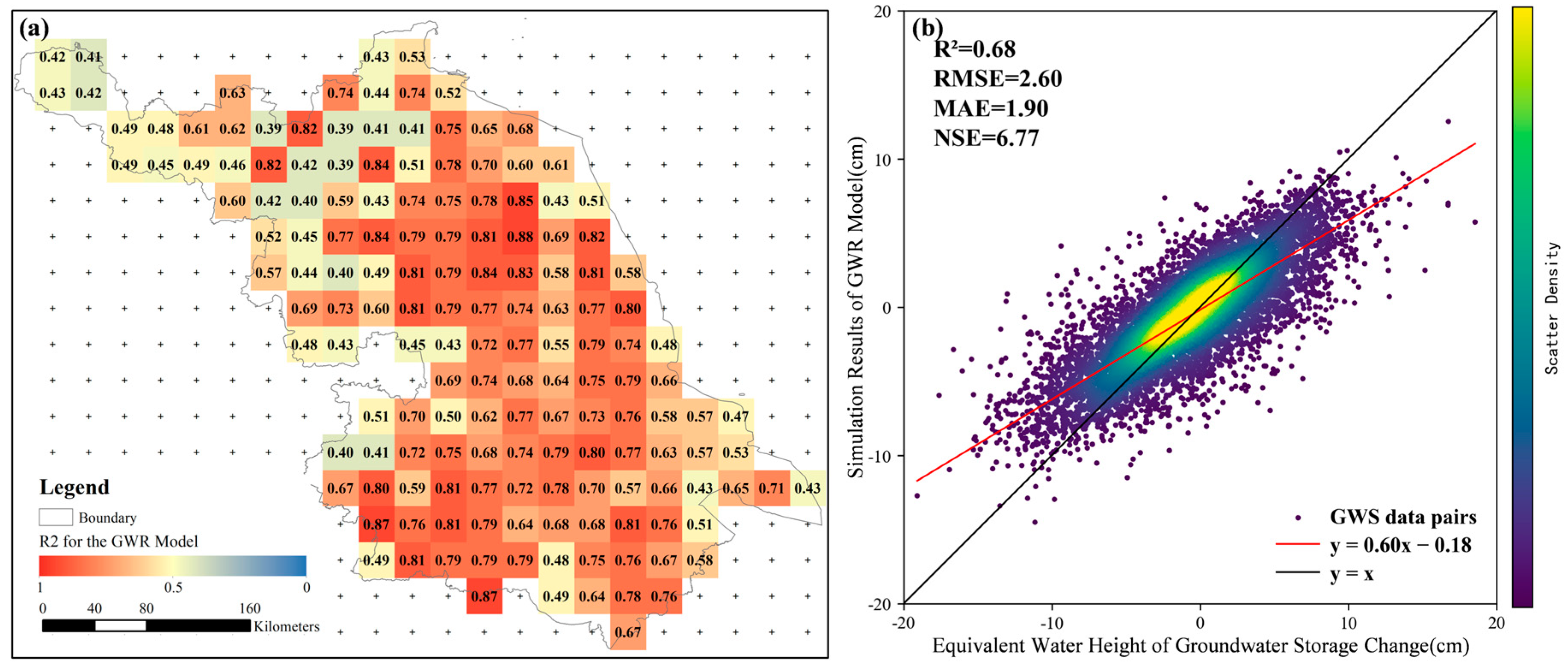
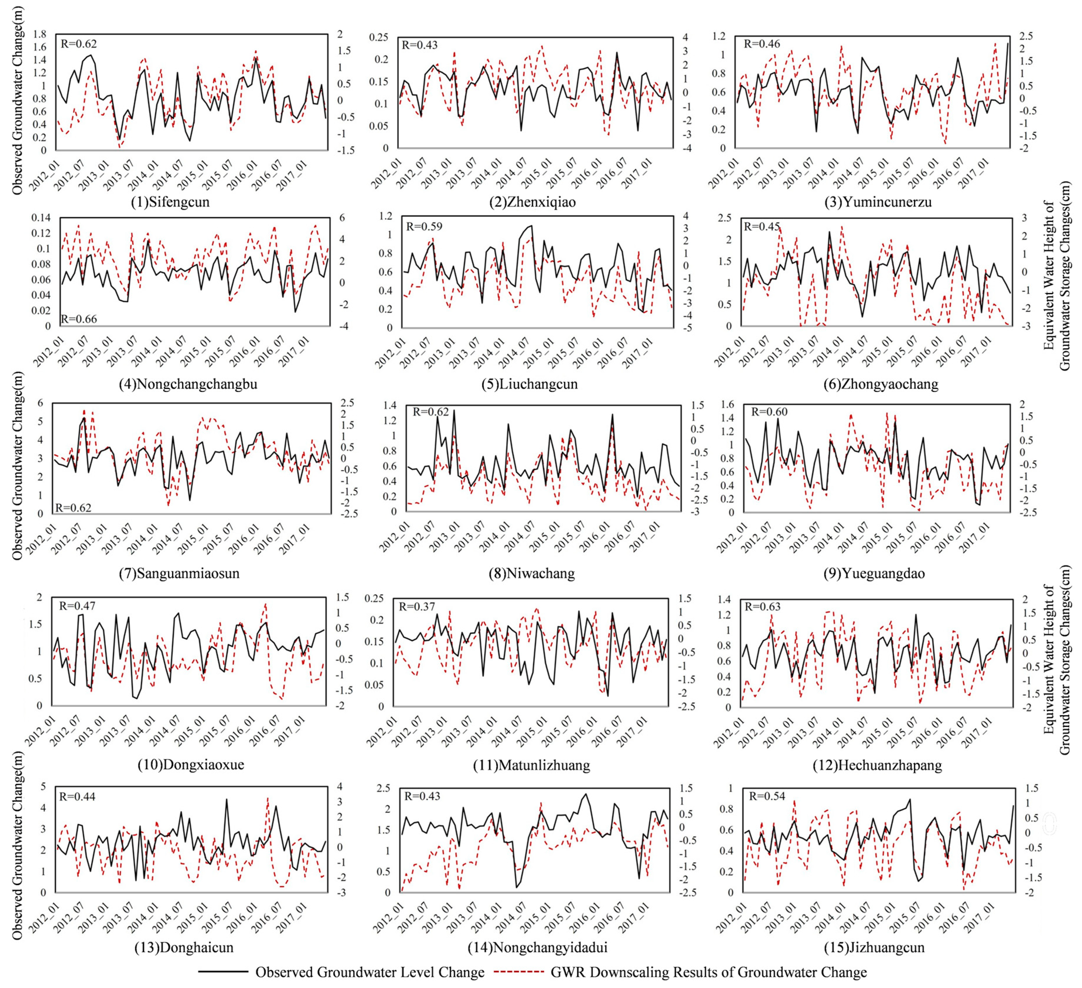
• GWR Model Accuracy Validation

Between January 2012 and June 2017, a total of 66 months of groundwater storage and explanatory variables at a 0.25° monthly scale were obtained for Jiangsu Province, with each month containing data from 158 grid cells. Based on these feature variables, this study used Gaussian functions as the kernel to measure spatial attenuation effects, and selected the optimal bandwidth by finding the optimal Akaike Information Criterion (AIC) value. AIC is a balance between model fitting goodness and complexity. In the process of bandwidth selection, for each possible bandwidth value, the AIC value of the corresponding bandwidth is calculated, and the bandwidth that minimizes the AIC value is selected as the optimal bandwidth based on the optimization principle of gradient descent. Finally, we used Python’s mgwr package to complete the construction of the GWR model, and the accuracy of the downscaling results is shown in Figure 5 and monthly in Figure S1. The output R² values ranged from approximately 0.39 to 0.88, and the root mean squared error (RMSE) reached around 2.6 cm. The proportion of GWR models with R² values below 0.5 was 18.52%, which may be attributed to the interpolation of the original data and error accumulation. Considering the data foundation and the overall range of R² values, this study concluded that the overall accuracy of the GWR downscaling model is acceptable.

2.

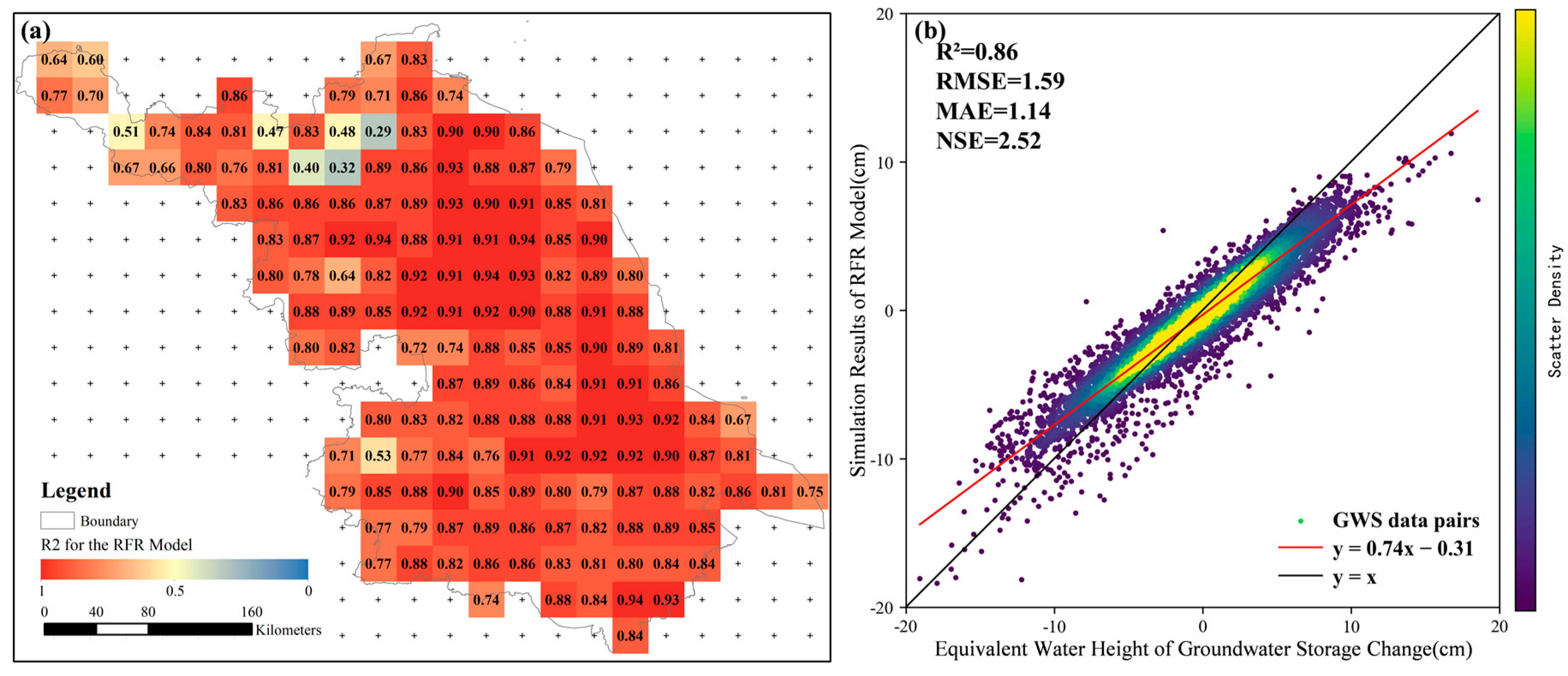
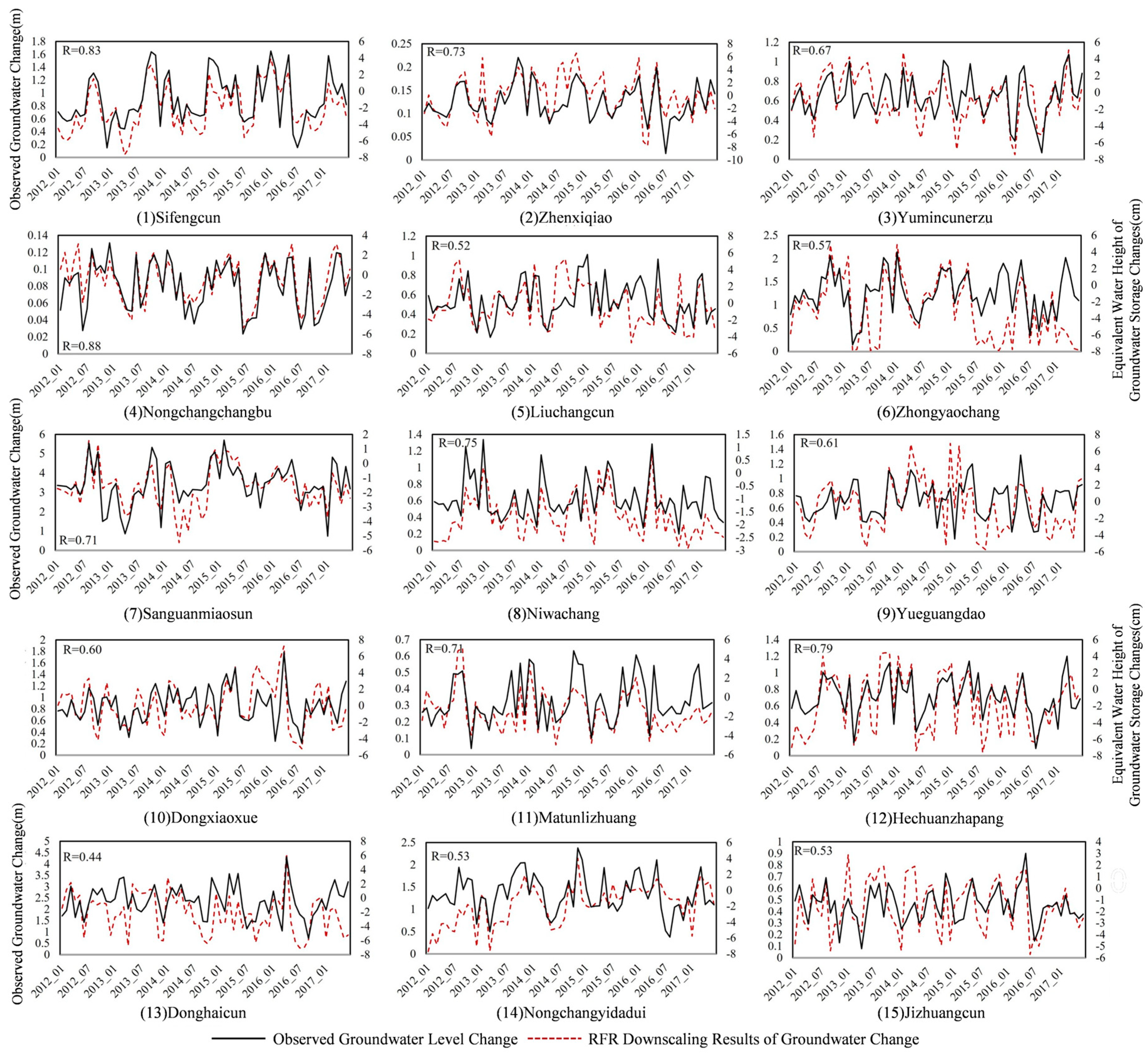
RFR Model Accuracy Validation

Consistent with the GWR model, this study extracted time series results from all 10,428 grids to train the RFR downscaling model, randomly selecting 30% of the sequence data as a test set. Additionally, a grid search coupled with a five-fold cross-validation was employed to optimize the hyperparameters of the RFR model. Specifically, a hyperparameter grid was defined firstly, enumerating all possible combinations of the hyperparameters to be tuned and their respective candidate values. The training dataset was subsequently partitioned into five subsets, with each subset serving as a validation set in turn. Model performance was evaluated for every hyperparameter combination across these folds, enabling the identification of the optimal hyperparameter configuration. Following optimization, the Random Forest model was configured with the number of regression trees (n_estimators) set to 400, the minimum sample number for splitting (min_samples_split) set to 5, and the minimum leaf number (min_samples_leaf) set to 2, while all other parameters remained at their default values. In this study, the RFR model trained on the 10,428 time series grid data achieved an average R² of 0.86, with the RMSE fluctuating around 1.59 cm, as shown in Figure 6, indicating that the model’s explanatory capability for the target variable reached a moderate level. Furthermore, the R² reached a maximum of 0.94. To better illustrate the monthly model accuracy, we have also plotted the monthly R²; in Figure S2. Taken together, the RFR model method is suitable for the downscaling analysis of groundwater storage in Jiangsu Province.

3.

Comparison of RFR and GWR Models

For the study area, although some regions of the GWR downscaling model exhibit an R² value below 0.5, overall, the accuracy of the GWR model is deemed acceptable. Additionally, the RFR model, trained on the time series data of 10,428 grids, achieved a coefficient of determination (R²) of 0.86, indicating that compared to the GWE model, the RFR model achieves a higher accuracy in predicting changes in regional groundwater storage (Figure S3). This model is suitable for downscaling analysis of groundwater storage in Jiangsu Province and can effectively predict changes in groundwater storage.

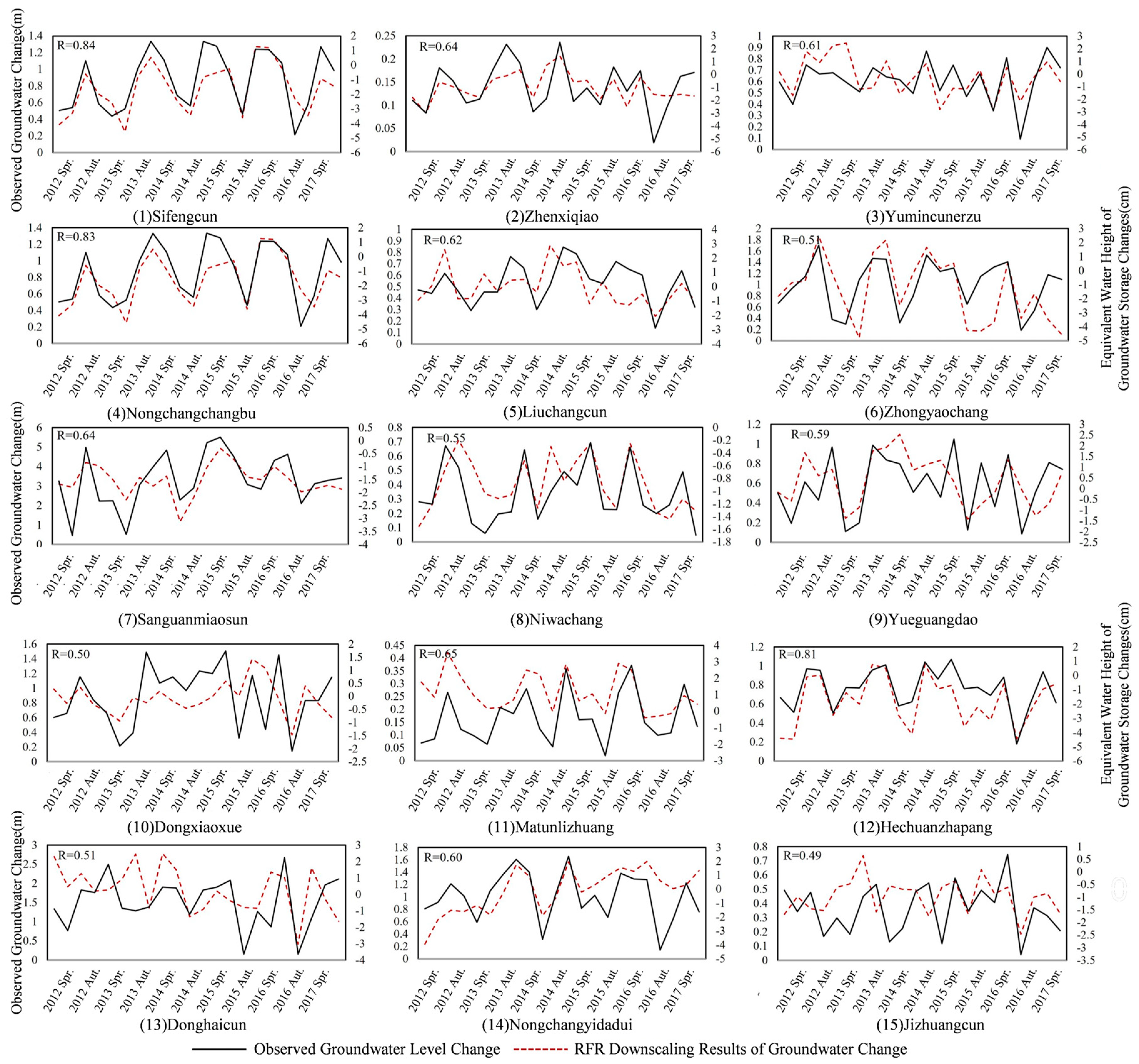
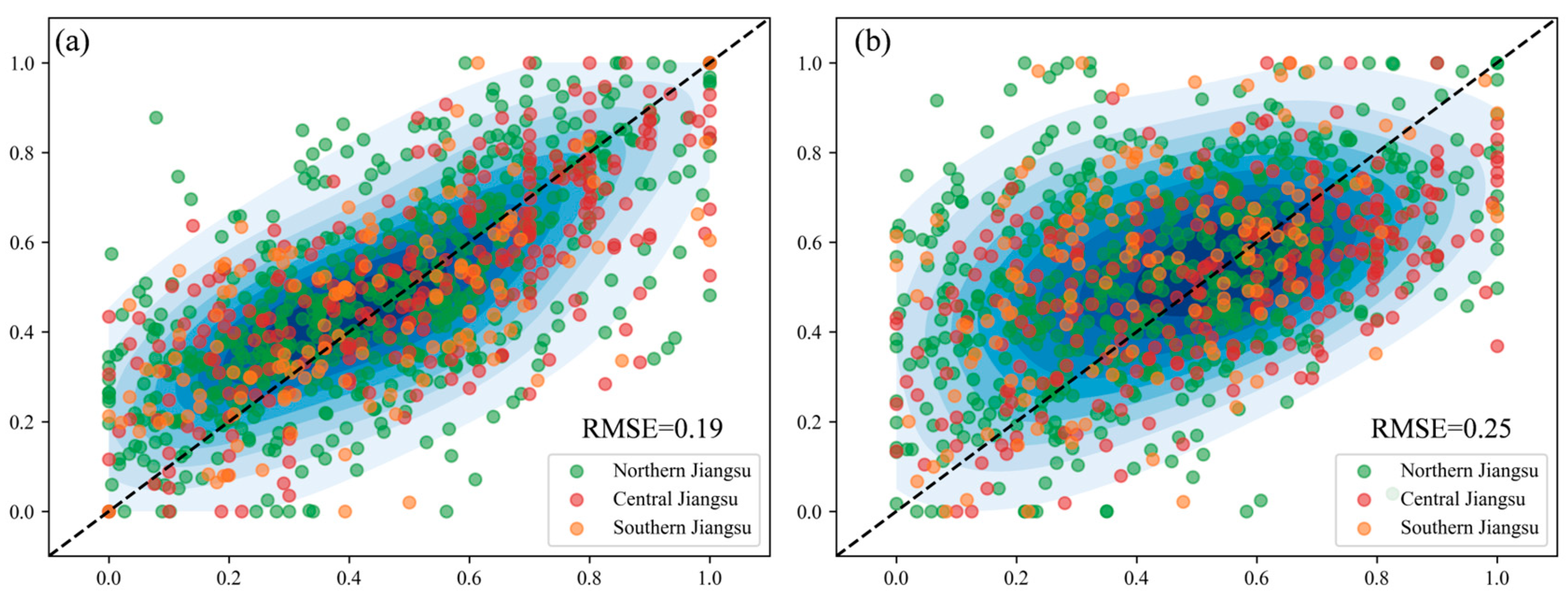
4.3.2. Downscaling Accuracy Validation

In this study, measured groundwater level data were selected to verify the reliability of the aforementioned regression models in downscaling the results of groundwater storage changes in Jiangsu Province. Due to insufficient temporal continuity of the observed water level data from ground stations between January 2012 and June 2017, this study removed stations with significant data gaps and used linear interpolation to fill in the missing data for stations with fewer gaps. Ultimately, a total of 15 groundwater level observation stations were available for validating the downscaling model results.

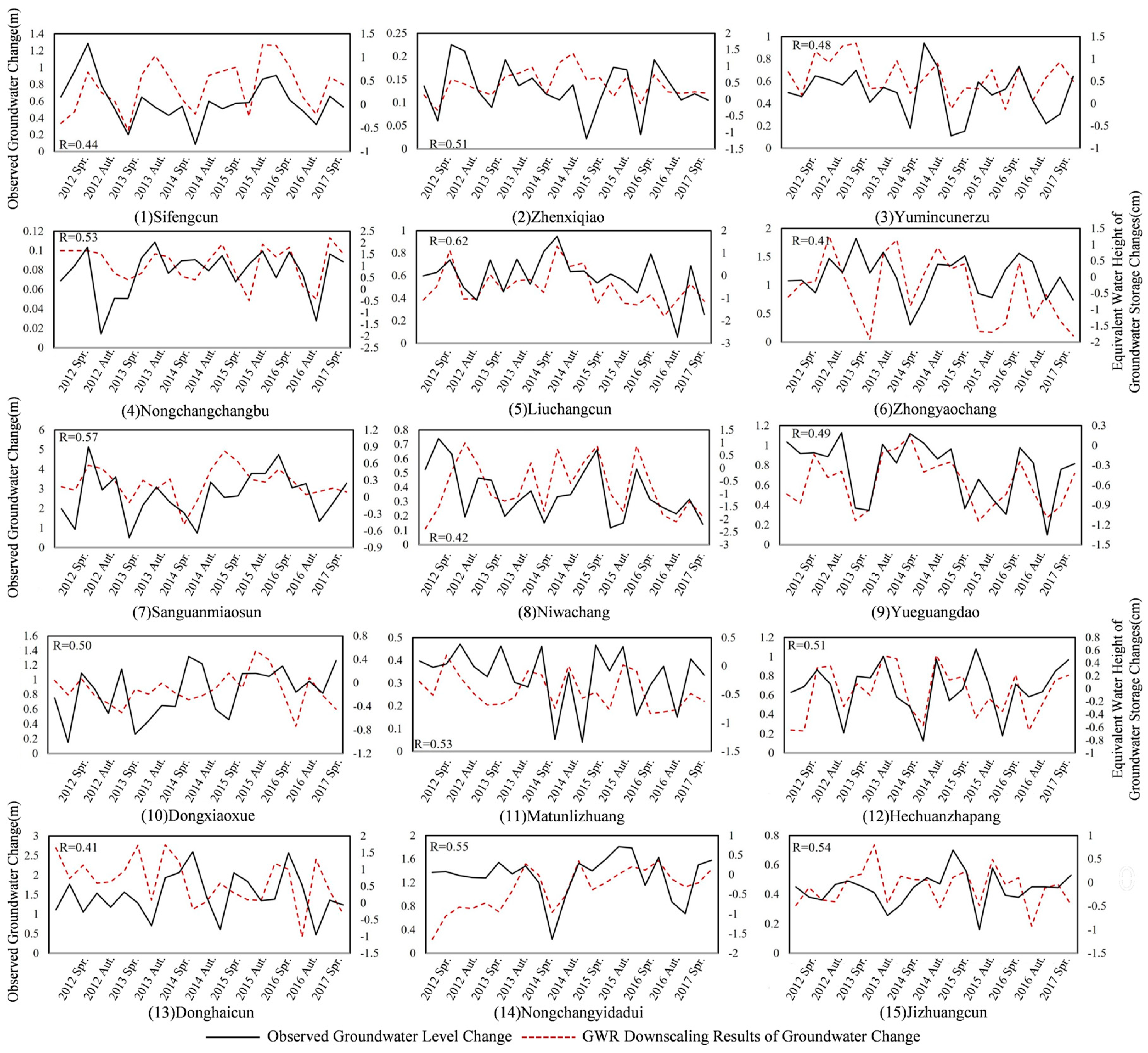
• Downscaling validation based on the GWR model

In this study, six representative months between January 2012 and June 2017 were selected to plot the original groundwater storage changes and the downscaled groundwater storage changes in Jiangsu Province. The downscaling performance of the GWR model was analyzed and compared, as shown in Figure 7. The GWR downscaling results obtained in this study generally reflect the spatial distribution of groundwater storage changes in Jiangsu Province. To some extent, these results are consistent with the overall characteristics of groundwater storage changes at the original resolution. The spatial variations exhibit good continuity, and the local-scale changes reveal more detailed features, though some discrepancies may occur. Meanwhile, compared to the original groundwater storage change data, the GWR downscaling results show fewer drastic fluctuations between high and low values, with smoother boundaries in groundwater storage changes.

We used the data from 15 groundwater level monitoring stations located in Xuzhou, Yangzhou, Suqian, Changzhou, and Taizhou, Jiangsu Province, to verify the accuracy and precision of the GWR model’s downscaling results. The data from 15 groundwater level monitoring stations located in Xuzhou, Yangzhou, Suqian, Changzhou, and Taizhou, Jiangsu Province, were used to verify the accuracy and precision of the GWR model’s downscaling results. Based on the latitude and longitude information of each station, the downscaled grid data for groundwater storage changes in the corresponding regions could be extracted and averaged. The following analysis sequentially show the correlation coefficients between the monthly and seasonal GWR downscaling results and the observed groundwater level fluctuation time series data.

As shown in Figure 8, among the 15 monthly-scale groundwater monitoring stations in Jiangsu Province, the correlation coefficients between the measured and GWR-predicted groundwater storage changes were below 0.5 at seven stations: Zhenxiqiao, Yumincunerzu, Zhongyaochang, Dongxiaoxue, Matunlizhuang, Donghaicun, and Nongchangyidadui, with most values around 0.45. Matunlizhuang had the lowest correlation, which was 0.37, indicating that the GWR model’s predictive accuracy in these areas was insufficient in explaining actual groundwater storage changes. In contrast, six stations: Sifengcun, Sanguanmiaosun, Nongchangchangbu, Niwachang, Yueguangdao, and Hechuanzhapang, had correlation coefficients above 0.60, suggesting that the GWR-predicted results were generally able to describe the actual groundwater fluctuations. Among these, the Liuchangcun and Jizhuangcun stations showed the highest correlations.

As shown in Figure 9, for the 15 seasonal-scale validation results, Jizhuangcun had the highest correlation coefficient, indicating a strong relationship between measured and predicted values. Additionally, eight stations (Matunlizhuang, Nongchangyidadui, Nongchangchangbu, Jizhuangcun, Zhenxiqiao, Hechuanzhapang, Sanguanmiaosun, and Dongxiaoxue) showed positive correlations above 0.5, demonstrating strong predictability for groundwater changes. However, six stations—Yueguangdao, Sifengcun, Yumincunerzu, Donghaicun, Zhongyaochang, and Niwachang—had correlation coefficients below 0.5, with Donghaicun and Zhongyaochang having the lowest at 0.41. Analysis of the time-series graphs showed consistent seasonal fluctuation patterns in groundwater levels and groundwater storage changes across all stations.

2.

Downscaling validation based on the RFR model

With the same approach as the GWR model, six representative months between January 2012 and June 2017 were selected to plot the original groundwater storage changes and the downscaled groundwater storage changes in Jiangsu Province. The downscaling performance of the RFR model was analyzed and compared, as shown in Figure 10. The RFR downscaling results, like those of the GWR, can also generally reflect the spatial distribution of groundwater storage changes in Jiangsu Province. Additionally, there are fewer abrupt fluctuations in high and low values, and the boundaries of groundwater storage changes are smoother.

In the same manner as for GWR, we also utilized 15 groundwater monitoring stations in Jiangsu Province to validate the accuracy and precision of the RFR model downscaling results. The following paragraph sequentially show the correlation coefficients between the monthly and seasonal RFR downscaling results and the observed groundwater level fluctuation time series data.

Analysis of the correlation coefficients between the observed and results of downscaled groundwater time series for monthly and seasonal scales in Jiangsu Province reveals that the range of correlation coefficients for the monthly time series data is between 0.44 and 0.88, while for the seasonal time series data, it is between 0.49 and 0.84 (Figure 11). Except for the Donghaicun station at the monthly scale and the Jizhuangcun station at the seasonal scale, where the correlation coefficients did not exceed 0.5, all other stations had correlation coefficients above 0.5. This indicates that the RFR downscaled results are strongly correlated with the water level fluctuations at the monitoring stations, demonstrating that the RFR model’s downscaling performance for groundwater storage changes in Jiangsu Province is acceptable.

As shown in Figure 12, Among the 15 verification results for Jiangsu Province, the correlation coefficients for Sifengcun at the monthly and seasonal scales reached 0.8 and 0.84, respectively, indicating the strongest correlation. Analysis of Figure 9 and Figure 10 shows that the groundwater storage in the Sifengcun area exhibited an overall upward trend, with clear seasonal fluctuations. In contrast, both Donghaicun and Jizhuangcun showed no significant correlation at either the monthly or seasonal scales. A comparison of the time series plots suggests that the larger fluctuations in observed groundwater levels at these stations might be due to the interpolation effects from missing data. For the other stations, the differences between monthly and seasonal scales were minor, and the correlation levels remained stable. Analyzing the time series plots reveals that groundwater level variations at each station generally follow the trends of groundwater storage changes.

In conclusion, the analysis of the monthly and seasonal scale time series plots and correlation results between observed groundwater level fluctuations and equivalent water height changes in groundwater storage in Jiangsu Province shows that the overall trends of the observed groundwater levels and the inversed groundwater storage changes in equivalent water height are largely consistent, with minimal differences in fluctuations. The findings suggest that using GRACE and GLDAS data offers significant advantages for groundwater storage monitoring in Jiangsu Province, while the spatial statistical downscaling method applied in this study demonstrates high reliability and accuracy. Overall, the downscaling approach based on the RFR model not only enhances the spatial resolution of groundwater storage changes but also ensures the accuracy of the predictive data.

3.

Comparison of RFR and GWR models in downscaling

The correlation coefficients between the downscaled time series of both the GWR and RFR models and the observed data indicate a positive relationship, with most of the stations having coefficients exceeding 0.5. This suggests that the downscaling models can accurately predict the change of groundwater storage in Jiangsu Province, showing that the downscaling methods improve spatial resolution while maintaining predictive accuracy. In both the monthly and seasonal scale validation results, some stations did not reach a correlation coefficient of 0.5, implying that the models’ ability to explain actual groundwater storage changes in these areas was limited, likely due to data-quality issues or accumulated errors. However, the fact that the correlation coefficients for most stations exceeded 0.5 indicates that the models’ predictions of groundwater changes are reasonably reliable in most cases.

Based on the correlation coefficients from the validation results, we can evaluate the performance of the GWR and RFR models in downscaling predictions. It is important to note that although the GWR model can generally predict changes in groundwater storage, its prediction accuracy is still limited in certain areas where the correlation coefficient did not reach 0.5. In comparison, the RFR model showed higher correlations at these stations, especially in the seasonal scale validation results.

The GWR model takes into account the spatial correlation and spatial heterogeneity of the feature dataset, dividing the feature data into multiple local regions. It fits a regression model for each region and uses a distance function to characterize the continuous spatial distribution. The RFR model is an ensemble learning method that does not take into account the spatial distribution and structure of features. In the modeling process, we already conducted independent modeling for different pixels. When the spatial correlation of feature data intersects, sample data is sparsely distributed, and when spatial resolution is low, the GWR model tends to be less reliable than the RFR model due to the weaker spatial association between samples. Considering the performance of both GWR and RFR models in downscaling prediction, it can be concluded that the RFR downscaling method offers certain advantages in monitoring groundwater storage changes in Jiangsu Province, particularly in improving spatial resolution and ensuring prediction accuracy.

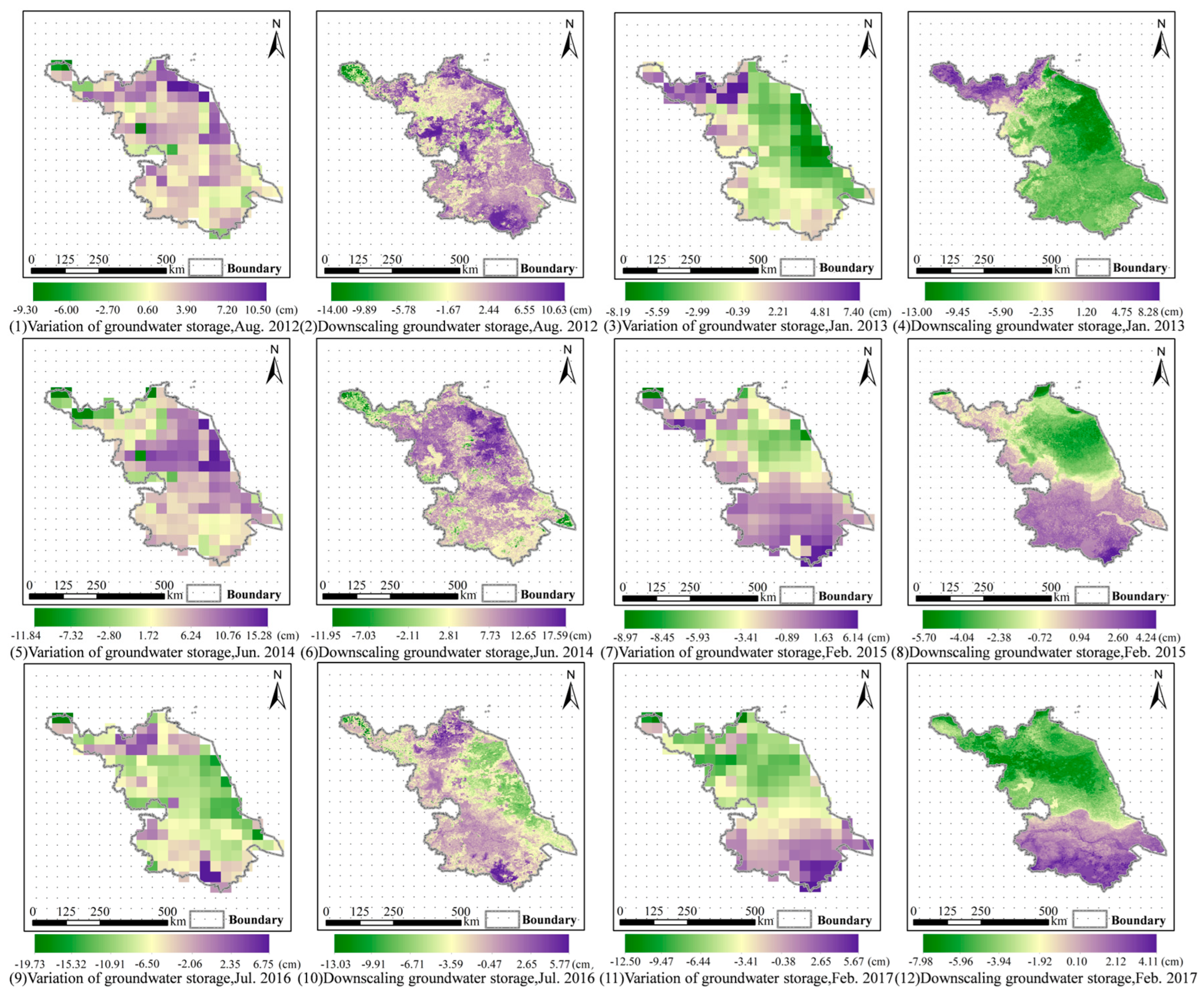
4.4. Spatial Distribution of Groundwater in Jiangsu Province

This study used the RFR downscaling results of groundwater storage changes in Jiangsu Province from January 2012 to June 2017 to obtain the monthly rate of change through linear fitting. Through zonal statistics, we calculated the monthly groundwater storage changes trend for various cities in Jiangsu from 2012 to 2017, as shown in Figure 13. The figure reveals a noticeable north–south difference in the spatial distribution of groundwater storage changes within Jiangsu Province. In the northern part of Jiangsu, near the North China Plain (northwest of Xuzhou City), groundwater storage shows an overall depletion, with severe losses, and the maximum rate of change exceeds 6.84 cm/month. This may be due to the high population density and large water consumption in the North China Plain. In contrast, in the southern part of Xuzhou, as well as in cities like Suzhou, Wuxi, and Changzhou (around the Taihu Lake Basin), groundwater storage increased to some extent, with rates of change between 0.5 and 1.89 cm/month. Meanwhile, in central Jiangsu, including cities such as Huai’an, Suqian, Lianyungang, and Yancheng, overall groundwater depletion is relatively mild and more balanced, with rates of change ranging from 0.5 to 2.5 cm/year.

From January 2012 to June 2017, in various cities of Jiangsu Province, the application of RFR downscaling enhanced the visibility of groundwater storage changes across the province. The high-resolution data obtained through downscaling was able to capture regional groundwater spatial fluctuations that were not observable in coarse-resolution data, showing strong spatial heterogeneity and temporal variation. For example, in Suzhou, Wuxi, and Taizhou, groundwater storage increased by 0.18 ± 0.048 cm/month, 0.15 ± 0.034 cm/month, and 0.12 ± 0.012 cm/month, respectively. This indicates that improvements in water conservation and efficiency, along with reductions in agricultural and industrial water losses, have promoted positive changes in regional groundwater storage. Additionally, the groundwater storage derived from GRACE, which showed uniform spatial distribution at the pixel scale in areas like Yancheng and Lianyungang, was better represented through RFR downscaling. The downscaling results provided a more accurate spatial distribution of regional groundwater changes in these areas.

5. Discussion

5.1. Comparison of GWR and RFR in Downscaling Modeling

This study simultaneously simulated groundwater storage changes in Jiangsu Province using both GWR and RFR models which enhanced the spatial resolution of groundwater storage data from 0.25° to 0.01°. The aim was to compare the application of spatial explicit models and traditional statistical models in groundwater downscaling, using these two classic models as examples. Groundwater depth is influenced by regional groundwater storage as well as geological characteristics such as aquifer porosity and thickness. To compare the simulation accuracy of the two models, we normalized the model results from different regions and plotted scatter plots, as shown in Figure 14. The normalized RFR model downscaling results have a root mean square error (RMSE) of 0.19, while the GWR model downscaling results have an RMSE of 0.25. It is clear that the RFR model exhibits better accuracy in simulating groundwater downscaling for Jiangsu Province.

The Jiangsu Province can be divided into three regions: southern Jiangsu, central Jiangsu, and northern Jiangsu. Southern Jiangsu lies south of the Yangtze River, while central and northern Jiangsu are separated by the Huai River, which marks the boundary between the humid and semi-humid climate zones in China [55]. Therefore, in this study, we aimed to compare the downscaling accuracy of the two models in the northern, central, and southern regions of Jiangsu Province, in order to evaluate the transferability of the models in groundwater downscaling simulations.

Both models performed worst in the northern region of Jiangsu Province and achieved the best results in the southern region. Specifically, in the GWR model results, a significant overestimation of groundwater storage in the northern region was observed, with an RMSE value of 0.27. In contrast, both models exhibited smaller errors in the southern region, with the RFR model having the lowest RMSE value of 0.15, which was still superior to the simulation accuracy of GWR. For the GWR model, the best simulation performance was observed in the central region, with an RMSE value of 0.22, though it was still lower than that of RFR. From the perspective of specific monitoring stations, the GWR downscaling results showed monthly correlation coefficients ranging from 0.37 to 0.66, with 53.33% of stations having correlation coefficients greater than 0.5. The quarterly correlation coefficients ranged from 0.41 to 0.62, with 60% of stations having correlation coefficients greater than 0.5. The RFR downscaling results had correlation coefficients ranging from 0.44 to 0.88, and the quarterly correlation coefficients ranged from 0.49 to 0.84, with only one station having correlation coefficients below 0.5, showing similar results. Compared with the groundwater downscaling study by Huang Shangfu et al. using the GWR model in the North China Plain [31], this study suggests that when using the GWR model at a large scale (such as the 0.25° scale used in this study), a larger bandwidth is typically set to satisfy the GWR kernel function’s spatial correlation measurement requirements. This, in turn, tends to overestimate the spatial correlation between geographic objects which are far apart from each other, leading to higher errors during modeling [56]. Additionally, the limited number of groundwater monitoring wells in this study may have also contributed to larger errors.

“Everything is related to everything else, but near things are more related than distant things” [57]. Specifically, hydrometeorological data often exhibit significant spatial correlation and spatial heterogeneity. Therefore, one of the goals of this research was to compare spatially explicit models with other models that do not consider spatial heterogeneity. However, due to the complex interactions in hydrometeorology, it seems that simple linear models cannot adequately capture these relationships. Moreover, the spatial dependencies at larger scales may not be effectively captured by the kernel functions of GWR. As a result, in complex regions with multiple aquifers, the RFR model demonstrated superior simulation results compared to the GWR model in this study.

5.2. Spatial–Temporal Characteristics of Groundwater Storage of Jiangsu Province

The allocation and rational use of water resources have increasingly become an important reference for industrial layout and production planning [58]. This study used the center of gravity shift model to calculate the trend direction and distance of the center of gravity for both increasing and decreasing groundwater storage, thereby visually reflecting its spatial variation characteristics (Figure 15). Additionally, the Local Indicators of Spatial Association (LISA) were introduced to characterize the distribution patterns of groundwater changes.

From 2004 to 2022, the center of gravity for groundwater storage increase was distributed in the central and southern regions of Jiangsu, while the center of gravity for groundwater storage decrease was distributed in the central and northern regions of Jiangsu. Comparing the two, except for the period from 2007 to 2010, when the groundwater increase center in northern Jiangsu was positioned farther north than the decrease center, in other years, the groundwater increase center was always located south of the decrease center. The migration patterns of the two centers also showed clear differences. The increase center first migrated northwest and then southeast, while the decrease center first migrated southeast and then northwest. Specifically, the increase center migrated a maximum of 162.42 km northwest and 106.21 km southeast, while the decrease center migrated a maximum of 324.25 km southeast and 221.64 km northwest. This reflects a noticeable latitudinal difference in groundwater change patterns, which is consistent with traditional understanding. There are significant differences in the industrial structure between the northern and southern parts of Jiangsu, and the migration of groundwater centers may be closely related to high-water-consuming industries and heavy industrial development, as well as the distribution of underground aquifers.

The LISA clustering map visualizes the spatial concentration and spatial autocorrelation characteristics of groundwater storage within the region, showing areas of “high-high” or “low-low” clusters. From Figure 16, it can be seen that, except for 2004, where the “high-high” clusters were mainly located in central Jiangsu, the “high-high” clusters have primarily and consistently been distributed in the southern regions of Jiangsu. From the perspective of the watershed systems, this includes the Yangtze River system and the Taihu Lake system. The “low-low” clusters have shown a tendency to shift from central Jiangsu to northern Jiangsu, indicating that the Yishusi River system has experienced an increasing trend of groundwater storage depletion in recent years. The “low-high” and “high-low” clusters are rare, suggesting that other influencing factors, such as human activities and climate change, also play a role in groundwater storage changes.

Among these factors, human activities have a significant impact on groundwater storage variation. With the acceleration of urbanization and industrialization, groundwater extraction has increased significantly [59]. Furthermore, the spatially uneven development of industrial layouts and the concentration of water-intensive heavy industries have made these factors important in groundwater storage changes. Therefore, future studies should consider incorporating human activity factors in addition to the environmental variables considered in this research to provide a more detailed depiction of groundwater variations.

6. Conclusions

This study found that in Jiangsu Province, the downscaling of groundwater storage changes exhibits a clear north–south contrast. In the northwest of Jiangsu, near the North China Plain, primarily in Xuzhou, groundwater storage generally exhibits a declining trend. In contrast, other cities show an increasing trend in groundwater storage. For instance, in Suzhou, Wuxi, and Taizhou, groundwater storage increases at rates of 0.18 ± 0.048 cm/month, 0.15 ± 0.034 cm/month, and 0.12 ± 0.012 cm/month, respectively. Additionally, both GWR and RFR models demonstrated a positive correlation with measured groundwater level variations in downscaled predictions, with more than 50% of the stations showing a correlation coefficient above 0.5, indicating that the downscaling method improves spatial resolution while maintaining a certain level of predictive accuracy. However, in areas where the correlation coefficient did not reach 0.5, the models exhibited weaker explanatory power for actual groundwater storage changes. The RFR model showed higher correlations in the validation results, indicating that the RFR downscaling method offers an advantage in monitoring groundwater storage changes in Jiangsu Province, particularly in terms of predictive accuracy.

References

1. Cuthbert, M.O.; Gleeson, T.; Moosdorf, N.; Befus, K.M.; Schneider, A.; Hartmann, J.; Lehner, B. Global Patterns and Dynamics of Climate–Groundwater Interactions. Nat. Clim. Change 2019, 9, 137–141. [Google Scholar] [CrossRef]
2. Famiglietti, J.S. The Global Groundwater Crisis. Nat. Clim. Change 2014, 4, 945–948. [Google Scholar] [CrossRef]
3. Wang, H.; Wang, J. Sustainable Utilization of China’s Water Resources. Bull. Chin. Acad. Sci. 2012, 27, 352–358. [Google Scholar] [CrossRef]
4. de Graaf, I.E.M.; Gleeson, T.; Rens van Beek, L.P.H.; Sutanudjaja, E.H.; Bierkens, M.F.P. Environmental Flow Limits to Global Groundwater Pumping. Nature 2019, 574, 90–94. [Google Scholar] [CrossRef]
5. Wada, Y.; van Beek, L.P.H.; van Kempen, C.M.; Reckman, J.W.T.M.; Vasak, S.; Bierkens, M.F.P. Global Depletion of Groundwater Resources. Geophys. Res. Lett. 2010, 37. [Google Scholar] [CrossRef]
6. Jasechko, S.; Perrone, D. Global Groundwater Wells at Risk of Running Dry. Science 2021, 372, 418–421. [Google Scholar] [CrossRef]
7. Chen, Z.; Zang, X.; Ran, J.; Hu, B.; Zhou, B. Terrestrial Water Storage Changes in Pearl River Region Derived from the Latest Release Temporal Gravity Field Models. J. Geod. Geodyn. 2020, 40, 305–310. [Google Scholar] [CrossRef]
8. Guo, F.; Sun, Z.; Ren, F.; Wen, Y. Analysis of global water storage variation based on GRACE time-variable gravity during 2003–2013. Prog. Geophys. 2019, 34, 1298–1302. [Google Scholar] [CrossRef]
9. Sun, P.; Guo, C.; Wei, D. Estimating Terrestrial Water Storage Variations in Chile with the Effects of Earthquakes Deducted. Hydrol. Sci. J. 2023, 68, 1663–1679. [Google Scholar] [CrossRef]
10. Ran, Q.; Pan, Y.; Wang, Y.; Chen, L.; Xu, H. Estimation of annual groundwater exploitation in Haihe River Basin by use of GRACE satellite data. Adv. Sci. Technol. Water Res. 2013, 33. 42–46+67. [Google Scholar] [CrossRef]
11. Tu, M.; Liu, Z.; He, C.; Ren, Q.; Lu, W. Research progress of groundwater storage changes monitoring in China based on GRACE satellite data. Adv. Earth Sci. 2020, 35, 643–656. [Google Scholar] [CrossRef]
12. Sarkar, T.; Karunakalage, A.; Kannaujiya, S.; Chaganti, C. Quantification of Groundwater Storage Variation in Himalayan & Peninsular River Basins Correlating with Land Deformation Effects Observed at Different Indian Cities. Contrib. Geophys. Geod. 2022, 52, 1–52. [Google Scholar] [CrossRef]
13. Jasechko, S.; Seybold, H.; Perrone, D.; Fan, Y.; Shamsudduha, M.; Taylor, R.G.; Fallatah, O.; Kirchner, J.W. Rapid Groundwater Decline and Some Cases of Recovery in Aquifers Globally. Nature 2024, 625, 715–721. [Google Scholar] [CrossRef]
14. Rana, S.K.; Chamoli, A. GRACE-Derived Groundwater Variability and Its Resilience in North India: Impact of Climatic and Socioeconomic Factors. Hydrol. Sci. J. 2024, 69, 2159–2171. [Google Scholar] [CrossRef]
15. Yoshe, A.K. Water Availability Identification from GRACE Dataset and GLDAS Hydrological Model over Data-Scarce River Basins of Ethiopia. Hydrol. Sci. J. 2024, 69, 721–745. [Google Scholar] [CrossRef]
16. Cho, Y. Analysis of Terrestrial Water Storage Variations in South Korea Using GRACE Satellite and GLDAS Data in Google Earth Engine. Hydrol. Sci. J. 2024, 69, 1032–1045. [Google Scholar] [CrossRef]
17. Su, H.; Zhang, G.; Zhang, D.; Yin, W.; Meng, X. Improving the spatial resolution of GRACE satellites based on high-resolution hydrological simulations. Bull. Surv. Mapp. 2022, 8, 41–47. [Google Scholar] [CrossRef]
18. Atkinson, P.M. Downscaling in Remote Sensing. Int. J. Appl. Earth Obs. Geoinf. 2013, 22, 106–114. [Google Scholar] [CrossRef]
19. Shokri, A.; Walker, J.P.; van Dijk, A.I.J.M.; Pauwels, V.R.N. On the Use of Adaptive Ensemble Kalman Filtering to Mitigate Error Misspecifications in GRACE Data Assimilation. Water Resour. Res. 2019, 55, 7622–7637. [Google Scholar] [CrossRef]
20. Zaitchik, B.F.; Rodell, M.; Reichle, R.H. Assimilation of GRACE Terrestrial Water Storage Data into a Land Surface Model: Results for the Mississippi River Basin. J. Hydrometeorol. 2008, 9, 535–548. [Google Scholar] [CrossRef]
21. Shokri, A.; Walker, J.P.; van Dijk, A.I.J.M.; Pauwels, V.R.N. Performance of Different Ensemble Kalman Filter Structures to Assimilate GRACE Terrestrial Water Storage Estimates Into a High-Resolution Hydrological Model: A Synthetic Study. Water Resour. Res. 2018, 54, 8931–8951. [Google Scholar] [CrossRef]
22. Zhang, M.; Hu, L. Research Progress on Statistical Downscaling Method. South-North Water Transf. Water Sci. Technol. 2013, 11, 118–122. [Google Scholar]
23. Tourian, M.J.; Saemian, P.; Ferreira, V.G.; Sneeuw, N.; Frappart, F.; Papa, F. A Copula-Supported Bayesian Framework for Spatial Downscaling of GRACE-Derived Terrestrial Water Storage Flux. Remote Sens. Environ. 2023, 295, 113685. [Google Scholar] [CrossRef]
24. Yazdian, H.; Salmani-Dehaghi, N.; Alijanian, M. A Spatially Promoted SVM Model for GRACE Downscaling: Using Ground and Satellite-Based Datasets. J. Hydrol. 2023, 626, 130214. [Google Scholar] [CrossRef]
25. Sahour, H.; Sultan, M.; Vazifedan, M.; Abdelmohsen, K.; Karki, S.; Yellich, J.; Gebremichael, E.; Alshehri, F.; Elbayoumi, T. Statistical Applications to Downscale GRACE-Derived Terrestrial Water Storage Data and to Fill Temporal Gaps. Remote Sens. 2020, 12, 533. [Google Scholar] [CrossRef]
26. Zhang, J.; Liu, K.; Wang, M. Downscaling Groundwater Storage Data in China to a 1-Km Resolution Using Machine Learning Methods. Remote Sens. 2021, 13, 523. [Google Scholar] [CrossRef]
27. Kalu, I.; Ndehedehe, C.E.; Ferreira, V.G.; Janardhanan, S.; Currell, M.; Crosbie, R.S.; Kennard, M.J. Remote Sensing Estimation of Shallow and Deep Aquifer Response to Precipitation-Based Recharge Through Downscaling. Water Resour. Res. 2024, 60, e2024WR037360. [Google Scholar] [CrossRef]
28. Ali, S.; Khorrami, B.; Jehanzaib, M.; Tariq, A.; Ajmal, M.; Arshad, A.; Shafeeque, M.; Dilawar, A.; Basit, I.; Zhang, L.; et al. Spatial Downscaling of GRACE Data Based on XGBoost Model for Improved Understanding of Hydrological Droughts in the Indus Basin Irrigation System (IBIS). Remote Sens. 2023, 15, 873. [Google Scholar] [CrossRef]
29. Kalu, I.; Ndehedehe, C.E.; Ferreira, V.G.; Kennard, M.J. Machine Learning Assessment of Hydrological Model Performance under Localized Water Storage Changes through Downscaling. J. Hydrol. 2024, 628, 130597. [Google Scholar] [CrossRef]
30. Wang, Y.; Li, C.; Cui, Y.; Cui, Y.; Xu, Y.; Hora, T.; Zaveri, E.; Rodella, A.-S.; Bai, L.; Long, D. Spatial Downscaling of GRACE-Derived Groundwater Storage Changes across Diverse Climates and Human Interventions with Random Forests. J. Hydrol. 2024, 640, 131708. [Google Scholar] [CrossRef]
31. Huang, S.; Duan, G.; He, J. Groundwater storage downscaling in the Hai River Basin based on the GWR model. Hydrop. Energy Sci. 2023, 41, 39–42+30. [Google Scholar] [CrossRef]
32. Chen, Z.; Zheng, W.; Yin, W.; Li, X.; Zhang, G.; Zhang, J. Improving the Spatial Resolution of GRACE-Derived Terrestrial Water Storage Changes in Small Areas Using the Machine Learning Spatial Downscaling Method. Remote Sens. 2021, 13, 4760. [Google Scholar] [CrossRef]
33. Janowicz, K.; Gao, S.; McKenzie, G.; Hu, Y.; Bhaduri, B. GeoAI: Spatially Explicit Artificial Intelligence Techniques for Geographic Knowledge Discovery and Beyond. Int. J. Geogr. Inf. Sci. 2020, 34, 625–636. [Google Scholar] [CrossRef]
34. Jiangsu Provincial Water Resources Department. Jiangsu Province Water Resources Bulletin-2023; China Water & Power Press: Beijing, China, 2024. [Google Scholar]
35. Wu, A. Annual Report on Groundwater Levels Monitoring of Geological Environment in China-2012; China Land Press: Beijing, China, 2013. [Google Scholar]
36. Wu, A. Annual Report on Groundwater Levels Monitoring of Geological Environment in China-2013; China Land Press: Beijing, China, 2014. [Google Scholar]
37. Wu, A. Annual Report on Groundwater Levels Monitoring of Geological Environment in China-2014; China Land Press: Beijing, China, 2016. [Google Scholar]
38. Wu, A. Annual Report on Groundwater Levels Monitoring of Geological Environment in China-2015; China Land Press: Beijing, China, 2017. [Google Scholar]
39. Peng, S. 1-Km Monthly Mean Temperature Dataset for China (1901–2021); National Tibetan Plateau/Third Pole Environment Data Center (TPDC): Beijing, China, 2019. [Google Scholar] [CrossRef]
40. Qu, L.; Zhu, Q.; Zhu, C.; Zhang, J. Monthly Precipitation Data Set with 1 Km Resolution in China from 1960 to 2020. Sci. Data Bank 2022. [Google Scholar] [CrossRef]
41. Peng, S.; Ding, Y.; Liu, W.; Li, Z. 1 Km Monthly Temperature and Precipitation Dataset for China from 1901 to 2017. Earth Syst. Sci. Data 2019, 11, 1931–1946. [Google Scholar] [CrossRef]
42. Jin, S.; Feng, G. Large-Scale Variations of Global Groundwater from Satellite Gravimetry and Hydrological Models, 2002–2012. Glob. Planet. Change 2013, 106, 20–30. [Google Scholar] [CrossRef]
43. Long, D.; Yang, W.; Sun, Z.; Cui, Y.; Zhang, C.; Cui, Y. GRACE satellite-based estimation of groundwater storage changes and water balance analysis for the Haihe River Basin. J. Hydraul. Eng. 2023, 54, 255–267. [Google Scholar] [CrossRef]
44. Brunsdon, C.; Fotheringham, S.; Charlton, M.E. Geographically Weighted Regression: A Method for Exploring Spatial Nonstationarity. Geogr. Anal. 1996, 28, 281–298. [Google Scholar] [CrossRef]
45. Salmerón, R.; García, C.B.; García, J. Variance Inflation Factor and Condition Number in Multiple Linear Regression. J. Stat. Comput. Simul. 2018, 88, 2365–2384. [Google Scholar] [CrossRef]
46. Foody, G.M. Geographical Weighting as a Further Refinement to Regression Modelling: An Example Focused on the NDVI–Rainfall Relationship. Remote Sens. Environ. 2003, 88, 283–293. [Google Scholar] [CrossRef]
47. Zhang, B.; Zhang, Y.; Gu, C.; Wei, B. Land cover classification based on random forest and feature optimism in the Southeast Qinghai-Tibet Plateau. Sci. Geogr. Sin. 2023, 43, 388–397. [Google Scholar] [CrossRef]
48. Li, M. Downscaling of GRACE-Derived Groundwater Storage Changes Based on Hierarchical Clustering and Non-Linear Regression Model. Master’s Thesis, Southwest Jiaotong University, Chengdu, China, 2021. [Google Scholar]
49. Shi, X.; Chen, Z.; Wang, H.; Yeung, D.-Y.; Wong, W.; Woo, W. Convolutional LSTM Network: A Machine Learning Approach for Precipitation Nowcasting. In Proceedings of the Advances in Neural Information Processing Systems 28 (NIPS 2015), Montreal, QC, Canada, 7–12 December 2015; Cortes, C., Lawrence, N.D., Lee, D.D., Sugiyama, M., Garnett, R., Eds.; Neural Information Processing Systems (nips): La Jolla, CA, USA, 2015; Volume 28. [Google Scholar]
50. Sun, L.; Guo, J.; Zhu, Y.; Chen, S. Feature Selection Using Stacking Integration and Partial Exploration Bayesian Optimization. J. Shanxi Univ. (Nat. Sci.) 2024, 47, 93–102. [Google Scholar] [CrossRef]
51. Ali, S.; Ran, J.; Luan, Y.; Khorrami, B.; Yun, X.; Tangdamrongsub, N. The GWR Model-Based Regional Downscaling of GRACE/GRACE-FO Derived Groundwater Storage to Investigate Local-Scale Variations in the North China Plain. Sci. Total Environ. 2024, 908, 168239. [Google Scholar] [CrossRef] [PubMed]
52. Xu, S.; Wu, C.; Wang, L.; Gonsamo, A.; Shen, Y.; Niu, Z. A New Satellite-Based Monthly Precipitation Downscaling Algorithm with Non-Stationary Relationship between Precipitation and Land Surface Characteristics. Remote Sens. Environ. 2015, 162, 119–140. [Google Scholar] [CrossRef]
53. Zhang, Y.; Liang, X.; Tian, Y.; Lin, J.; Wang, D. Analysis of temporal and spatial variation characteristics and driving factors of vegetation CUE in typical basin entering the sea in Beibu Gulf. Bull. Surv. Mapp. 2023, 8, 1–6. [Google Scholar] [CrossRef]
54. Bradley, P.E.; Keller, S.; Weinmann, M. Unsupervised Feature Selection Based on Ultrametricity and Sparse Training Data: A Case Study for the Classification of High-Dimensional Hyperspectral Data. Remote Sens. 2018, 10, 1564. [Google Scholar] [CrossRef]
55. Yang, X.; Li, D. Precipitation Variation Characteristics and Arid Climate Division in China. J. Arid Meteorol. 2008, 26, 17–24. [Google Scholar]
56. Cheng, C.; Wen, C.; Hai-xia, Z. Spatial Matching Pattern between Industrial Space and Ecological Protection in Areas along the Yangtze River in Jiangsu Province. Geogr. Res. 2011, 30, 269–277. [Google Scholar] [CrossRef]
57. Tobler, W.R. A Computer Movie Simulating Urban Growth in the Detroit Region. Econ. Geogr. 1970, 46, 234–240. [Google Scholar] [CrossRef]
58. Wang, Y.; Duan, X.; Wang, L. Spatial Distribution and Source Analysis of Heavy Metals in Soils Influenced by Industrial Enterprise Distribution: Case Study in Jiangsu Province. Sci. Total Environ. 2020, 710, 134953. [Google Scholar] [CrossRef] [PubMed]
59. Zhang, C.; Zhang, X.; Wu, Q.; Li, H. The Coordination About Quality and Scale of Urbanization: Case Study of Jiangsu Province. Sci. Geogr. Sin. 2013, 33, 16–22. [Google Scholar] [CrossRef]
Figure 1. (a) Location map of Jiangsu Province; (b) distribution map of groundwater monitoring stations used in this study; (c) distribution map of river system in Jiangsu Province.
Remotesensing 17 00493 g001
Figure 2. Research framework.
Remotesensing 17 00493 g002
Figure 3. Multicollinearity analysis of feature dataset (a) linear correlation of each feature; (b) VIF values for each explanatory variable.
Remotesensing 17 00493 g003
Figure 4. Analysis of feature contribution based on MDA in Random Forest.
Remotesensing 17 00493 g004
Figure 5. The accuracy validation of the GWR model: (a) spatial distribution of the coefficient of determination (R2) for GWR model results; (b) scatter plot of model simulation results and equivalent water height.
Remotesensing 17 00493 g005
Figure 6. The accuracy validation of the RFR model: (a) spatial distribution of the coefficient of determination (R2) for GWR model results; (b) scatter plot of model simulation results and equivalent water height.
Remotesensing 17 00493 g006
Figure 7. Comparison of groundwater storage changes before and after downscaling with GWR.
Remotesensing 17 00493 g007
Figure 8. The correlation analysis chart for the monthly groundwater level fluctuations and the GWR prediction results for Jiangsu Province.
Remotesensing 17 00493 g008
Figure 9. The correlation analysis chart for the seasonal groundwater level fluctuations and the GWR prediction results for Jiangsu Province.
Remotesensing 17 00493 g009
Figure 10. Comparison of groundwater storage changes before and after downscaling with RFR.
Remotesensing 17 00493 g010
Figure 11. The correlation analysis chart between the monthly groundwater level fluctuations and the RFR prediction results for Jiangsu Province.
Remotesensing 17 00493 g011
Figure 12. The correlation analysis chart for the seasonal groundwater level fluctuations and the RFR prediction results for Jiangsu Province.
Remotesensing 17 00493 g012
Figure 13. The map of the average monthly groundwater storage variation for each city in Jiangsu Province.
Remotesensing 17 00493 g013
Figure 14. Comparison of downscaling accuracy: (a) RFR model downscaling results; (b) GWR downscaling results.
Remotesensing 17 00493 g014
Figure 15. Center of gravity migration of groundwater storage changes in Jiangsu province: (a) center of gravity for groundwater storage increase; (b) center of gravity for groundwater storage decrease.
Remotesensing 17 00493 g015
Figure 16. LISA clustering map of groundwater storage variation for representative years from 2004 to 2022 in Jiangsu Province.
Remotesensing 17 00493 g016